Exploring the advantages of the maximum entropy model in calibrating cellular automata for urban growth simulation: a comparative study of four methods

ABSTRACT

As a powerful predictive technique based on machine learning, the maximum entropy (MaxEnt) model has been widely used in geographic modeling. However, its performance in calibrating cellular automata (CA) for urban growth simulation has not been investigated. This study compares the MaxEnt model with logistic regression (LR), artificial neural network (ANN), and support vector machine (SVM) models to explore its advantages in simulating urban growth and interpreting driving mechanisms. With the land use data of 2000 and 2020 from GlobeLand30, the constructed LR-CA, ANN-CA, SVM-CA, and MaxEnt-CA models are applied to simulate the urban growth of Beijing, Tianjin, and Wuhan, respectively. Their performance has been evaluated from multiple aspects such as the accuracy of training, testing, and projecting, computational efficiency, simulation accuracy, and simulated urban landscape. The results indicate that the MaxEnt model is superior to the other models except for the computational efficiency, but the time required for the MaxEnt training and projecting is acceptable and far less than that of the SVM. Taking the LR-CA as the benchmark, the kappa coefficients (Kappa) of the MaxEnt-CA have been increased by 4.20%, 3.38%, and 5.87% in Beijing, Tianjin, and Wuhan, respectively; the increments of corresponding figure of merits (FoM) are 6.26%, 4.58%, and 8.49%. The driving mechanisms of urban growth such as the interactions, response curves, and importance of spatial variables, have also been revealed by the MaxEnt modeling. The driving mechanisms of urban growth in Tianjin are more complex than that in Beijing and Wuhan, because there are more variable interactions; the relationships between spatial factors and urban growth in the three study areas are all nonlinear; the topographic factors and city center of Beijing, the traffic factors and water bodies of Tianjin, and the traffic factors, city center and water bodies of Wuhan are significant factors affecting their urban growth.

KEYWORDS:

• Cellular automata
• urban growth
• simulation
• maximum entropy model

1 Introduction

1.1 Literature review on cellular automata

As a general and powerful simulation model, cellular automata (CA) have been used to simulate urban growth from the 1970s (Tobler 1970). With the rapid development of 3S (Global Positioning System (GPS), remote sensing (RS), and geographic information system (GIS)) technologies, many CA models have been designed to model land use change processes (Sante et al. 2010; Aburas et al. 2016). In particular, the ability of GIS in spatial analysis and mathematical modeling is the key to the development and improvement of CA models (Stevens, Dragicevic, and Rothley 2007). The components of CA models have also been investigated and optimized in many aspects (Garcia et al. 2011; Li, Liu, and Yu 2014; Dahal and Chow 2015; Zhang and Wang 2021). The transition rule is the core of a CA model, and its ability to capture urban growth characteristics affects the performance of CA models (Sante et al. 2010; Roodposhti, Aryal, and Bryan 2019).

At first, transition rules were often built by experts based on subjective experiences, which was limited by their professional knowledge and impeded the development and application of CA models (Wu 2002). Moreover, such subjective rules can only describe urban growth characteristics that can be directly observed or speculated, and have no ability to mine hidden mechanisms (Sante et al. 2010; Li and Gong 2016). For example, the subjective rules in the studies of Tobler (1979) and White and Engelen (1993) were defined as: the potential to change the cell state in next time step was determined by surrounding land use types and their corresponding expert-defined weights. With the development of GIS, various spatial factors together with some methods that combine qualitative and quantitative analysis, such as multi-criteria evaluation (MCE) (Yu et al. 2011) and analytic hierarchy process (AHP) (Park, Jeon, and Choi 2012), have been used to generate the transition potential map (TPM), which is the essential component of subjective and objective rules. Although this kind of transition rules incorporates the influence of spatial factors into the derivation, it is limited by users’ expertise and cannot characterize nonlinear and complex mechanisms of urban growth (Aburas et al. 2016).

In recent years, as the development of computing technologies and machine learning, the TPM can be derived by training the samples drawn from spatial data, which improves its ability to capture urban growth characteristics (Li and Gong 2016). Many methods have been adopted to generate the TPM to build the data-driven rules of urban CA models, including but not limited to logistic regression (LR) (Munshi et al. 2014), support vector machine (SVM) (Rienow and Goetzke 2015), genetic algorithm (GA) (Garcia et al. 2013), ant colony optimization (ACO) (Li et al. 2011), particle swarm optimization (PSO) (Liao et al. 2014), artificial neural network (ANN) (Xu, Gao, and Coco 2019), and random forest (RF) (Kamusoko and Gamba 2015). For these data-driven methods, the representativeness of samples to the population data is an important factor affecting the performance of CA models, which has been explored in some studies (Li, Liu, and Yu 2014; Zhang and Xia 2021). In addition, the driving mechanisms learned from sample training also have crucial impacts on urban growth simulation. Original spatial variables related to urban growth are often used as training features, and their corresponding weights are obtained through sample training, which is the case for the training based on LR, GA, ACO, and PSO (Garcia et al. 2013; Munshi et al. 2014; Wang et al. 2021; Zhang and Wang 2021). The data-driven rules trained in this mode take each original spatial variable as the data element to describe urban dynamics, which limits the mining of driving mechanisms (Shen et al. 2016; Wang et al. 2018). Figure 1 depicts the classification of transition rules involved in this paper.

Figure 1. The classification of transition rules involved in this paper.

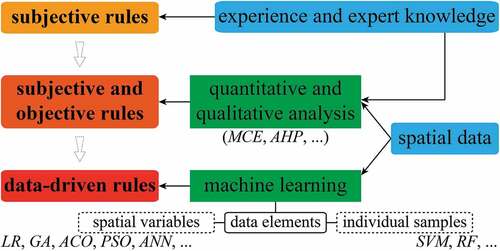
Furthermore, there are some methods that scale the original spatial variables or use individual samples as data elements to train the TPM. For example, in the training of the ANN, original spatial variables are nonlinearly transformed by activation functions, which improves the ability of the ANN to learn complex characteristics and solve nonlinear problems (Gundogdu et al. 2016). For the SVM training, each sample with features is mapped as a vector into a high-dimensional space, and the classification is performed by maximizing the margin between support vectors and the hyperplane (Ding, Hua, and Yu 2014). Most redundant vectors are ignored in the SVM training, and only a small number of crucial support vectors are used for the classification, which improves the robustness and generalizability of the SVM (Shen et al. 2016). Besides, as an ensemble learning method, RF couples random sampling and decision tree bagging to generate the TPM (Kamusoko and Gamba 2015). The RF training involves feature sampling and selection, and has an excellent performance on classification (Wang et al. 2018; Wu et al. 2021). However, ANN and SVM are black-box classifiers that cannot offer explicit interpretations of parameters and feature importance (Phillips et al. 2015). Although RF can evaluate and give the importance of spatial variables, it, as well as the ANN and SVM, cannot incorporate the variable interactions into training (Wright, Ziegler, and Konig 2016).

1.2 Maximum entropy model and research background

The maximum entropy (MaxEnt) model combines machine learning and feature engineering to predict unknown distributions based on the maximum entropy principle (Phillips, Anderson, and Schapire 2006). The maximum entropy principle evolved from the concept of information entropy (Shannon 1948) and was proposed by (Jaynes 1957, 1982). The mathematical formulation of the MaxEnt model is simple and precise, which makes its modeling mechanism easy to be interpreted (Elith et al. 2011). Feature engineering enables the MaxEnt model to incorporate diverse features to characterize the effects of spatial factors on urban growth, and to estimate the importance and interactions of spatial variables (Merow, Smith, and Silander 2013). The development of machine learning algorithms improves the efficiency of finding the approximate distribution with the maximum entropy, thereby enhancing the applicability of the MaxEnt model in many fields, such as signal processing (Mohammad-Djafari 2015), species distribution prediction (Phillips, Anderson, and Schapire 2006; Phillips and Dudik 2008), and image reconstruction and restoration (Prakash et al. 2018).

In recent years, the MaxEnt model has been gradually applied to the geographic modeling of land use change. For example, Wilson (2010) reviewed and prospected the application of the MaxEnt method in urban and regional modeling analysis; Zhang et al. (2020b) coupled the MaxEnt model and CA model to simulate the land use/cover change (LUCC) of China; Wang et al. (2020) used the MaxEnt model to optimize the stochastic component of CA models for urban growth simulation. They stated that the incorporation of the MaxEnt model was conducive to obtain better results (Wang et al. 2020; Zhang et al. 2020b). However, they did not further analyze and interpret the advantages of the MaxEnt model. Some recent studies have investigated and compared the performance of commonly used methods in urban growth simulation, which has promoted the development of CA models (Shafizadeh-Moghadam et al. 2017a, 2017b). Powerful data-driven methods are usually compared with other approaches to explore their merits in calibrating CA for urban growth simulation, such as ANN (Berberoglu, Akin, and Clarke 2016), SVM (Mustafa et al. 2018), GA and PSO (Feng, Liu, and Tong 2018). Moreover, homologous methods are often selected to investigate their differences in calibrating CA transition rules, such as spatially heterogeneous modeling approaches (Gao et al. 2020) and tree-based methods (Du et al. 2018). It can be concluded from these researches that simulation ability and interpretability are two major criteria for evaluating the performance of methods modeling urban growth (Du et al. 2018; Shafizadeh-Moghadam et al. 2021). Therefore, this study investigates two aspects of the MaxEnt modeling performance, namely, 1) the performance of simulating urban growth and 2) the ability to explicitly interpret driving mechanisms, to explore its advantages in urban growth simulation.

As described above, the powerful data-driven methods are widely used in most current studies (Li and Gong 2016), including but not limited to two categories of training modes: using spatial variables as data elements and using individual samples as data elements. ANN and SVM are the typical methods in these two categories respectively, and they have been widely used in urban growth simulation (Rienow and Goetzke 2015; Omrani, Tayyebi, and Pijanowski 2017; Karimi et al. 2019; Xu, Gao, and Coco 2019). Besides, LR is the most commonly used linear method to derive CA transition rules (Xia and Zhang 2021). Valuable discoveries and suggestions can be obtained by comparing the performance of LR, ANN, SVM, and MaxEnt methods. Therefore, four kinds of CA models are built to simulate the urban growth of Beijing, Tianjin, and Wuhan over the time period of 2000–2020, including the CA model based on MaxEnt (MaxEnt-CA), the CA model based on LR (LR-CA), the CA model based on ANN (ANN-CA), and the CA model based on SVM (SVM-CA). The advantages of the MaxEnt model in simulating urban growth have been discovered through comparing the performance of the four CA models. Moreover, its advantages in interpreting driving mechanisms have also been explained by analyzing the importance and interactions of spatial variables, and their relationships with urban growth.

Following the introduction, the remainder of this paper is structured as follows. Section 2 describes the study areas and datasets. Section 3 presents the mechanisms of the MaxEnt model to capture urban growth characteristics and generate the TPM. The methodologies of the LR, ANN, and SVM models, and the indicators for evaluating model performance and simulation results are also described in Section 3. Section 4 compares the training and simulation performance of the four models, and interprets the driving mechanisms of urban growth in the three study areas to indicate the advantages of the MaxEnt model. Section 5 discusses the advantages of the MaxEnt model in simulating urban growth and discovering driving mechanisms, and summarizes the findings and contributions of this paper. Section 6 presents our conclusions and describes some limitations and possible future work.

2 Study area and data

Beijing, Tianjin, and Wuhan are selected to investigate the advantages of the MaxEnt model in calibrating CA models. Beijing is the capital city and the political and cultural center of China, which is adjacent to the Taihang Mountains and located in the north of the North China Plain. By the end of 2019, the permanent resident population of Beijing was about 22 million, with an urbanization rate of 86%. Beijing has jurisdiction over 16 districts with a total area of 16,411 km², and has experienced a rapid urbanization process in recent decades (Beijing Municipal Bureau Statistics & Survey Office of the National Bureau of Statistics in Beijing, 2020). Tianjin is a municipality directly under the central government and the largest port city in the north of China; it is adjacent to Beijing in the west and the Bohai Sea in the east. By the end of 2019, the permanent resident population of Tianjin was about 16 million, with an urbanization rate of 83%. Tianjin has jurisdiction over 16 districts with a total area of 11,966 km² (Tianjin Municipal Bureau Statistics & Survey Office of the National Bureau of Statistics in Tianjin 2020). Convenient transportation and developed industrial foundation have greatly promoted the urbanization process of Tianjin in recent decades. Wuhan is the capital city of Hubei province and the largest city in central China. Wuhan has jurisdiction over 13 districts with a total area of 8,569 km². By the end of 2019, Wuhan had a permanent resident population of 11 million, and a gross domestic product (GDP) of 1,620 billion Yuan (Wuhan Municipal Statistics Bureau & State Statistical Bureau Wuhan Investigation Team 2020). In recent years, Wuhan has experienced a rapid urbanization process, which has played a significant role in promoting the development of surrounding cities.

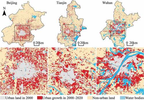
The land use dataset for the year 2000 and 2020 is obtained from GlobeLand30 (https://www.globallandcover.com); the vector dataset of road network for the year 2020 is obtained from OpenStreetMap (https://www.openstreetmap.org); and the dataset of digital elevation model (DEM) is obtained from EarthData (https://earthdata.nasa.gov). GlobeLand30 is supported by the National Geomatics Center of China (NGCC), it includes ten land categories, namely, artificial surface, cultivated land, forest, grassland, water bodies, shrubland, wetland, tundra, perennial snow and ice, and bare land. Many 30-meter resolution multispectral remote sensing images, such as multispectral images (TM5, ETM+, and OLI) of Landsat (USA) and multispectral images of the China Environment and Disaster Reduction Satellite (HJ-1), as well as the 16-meter resolution multispectral images of the China High Resolution Satellite (GF-1), were used for the production and update of GlobeLand30. After updating the land use data of 2020, the total accuracy of GlobeLand30 is 85.72%, and the Kappa coefficient is 0.82 (Chen et al. 2021). In this study, the artificial surface is regarded as the urban land, and the land use data are reclassified into three categories, namely, urban land, non-urban land, and water bodies. Figure 2 shows the urban growth of Beijing, Tianjin, and Wuhan during 2000–2020.

Figure 2. The urban growth of Beijing, Tianjin, and Wuhan during 2000–2020. The central zones of Beijing, Tianjin, and Wuhan have been enlarged to show details.

Referring to previous studies, some driving forces are selected to explain the urban growth in Beijing, Tianjin, and Wuhan, including proximity to different levels of administrative centers, proximity to roads, proximity to stations, and topographical conditions. Topographic factors such as slope and elevation are usually regarded as important driving factors that affect urban growth (Müller, Steinmeier, and Küchler 2010; Chettry and Surawar 2021). Proximity factors, such as distance to roads (Sante et al. 2010), distance to administrative centers (Vermeiren et al. 2012), and distance to water bodies (Zhang et al. 2020a) are also crucial driving factors that play a great role in the urbanization process. The details of spatial factors and corresponding spatial variables are shown in Table 1. The spatial variables used to model the urban growth of Beijing, Tianjin, and Wuhan are visualized in Figure 3, Figure 4, and Figure 5, respectively. It should be noted that all the spatial variables are linearly normalized into the range of 0 to 1 before being used for modeling. The linear normalization can be described as r’ = (max(r)-r)/(max(r)-min(r)), where r is the original value and r’ is the normalized value.

Figure 3. The spatial variables used to model the urban growth of Beijing, including dis2CC, dis2DC, dis2TC, dis2TRW, dis2PRW, dis2SEW, dis2TEW, dis2RST, dis2EEM, dis2WAB, Eleva, and Slope. Labels and units of spatial variables are explained in .Table 1

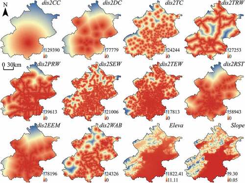
Figure 4. The spatial variables used to model the urban growth of Tianjin, including dis2CC, dis2DC, dis2TC, dis2TRW, dis2PRW, dis2SEW, dis2TEW, dis2RST, dis2EEM, dis2WAB, Eleva, and Slope. Labels and units of spatial variables are explained in .Table 1

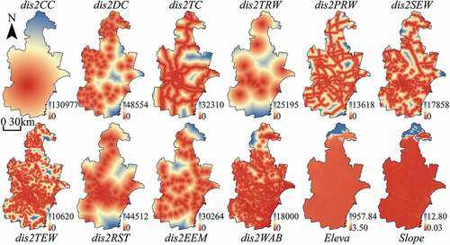
Figure 5. The spatial variables used to model the urban growth of Wuhan, including dis2CC, dis2DC, dis2TC, dis2TRW, dis2PRW, dis2SEW, dis2TEW, dis2RST, dis2EEM, dis2WAB, Eleva, and Slope. Labels and units of spatial variables are explained in .Table 1

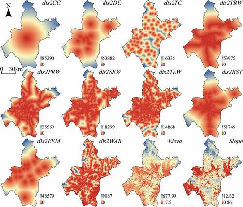
Table 1. The details of spatial factors and corresponding spatial variables

Dataset	Year	File type	Variable	Unit	Meaning	Source
City center	2020	Shapefile	dis2CC	Meter	Distance to city center	OpenStreetMap
District centers	2020	Shapefile	dis2DC	Meter	Distance to district centers	OpenStreetMap
Township centers	2020	Shapefile	dis2TC	Meter	Distance to township centers	OpenStreetMap
Trunk ways	2020	Shapefile	dis2TRW	Meter	Distance to trunk ways	OpenStreetMap
Primary ways	2020	Shapefile	dis2PRW	Meter	Distance to primary ways	OpenStreetMap
Secondary ways	2020	Shapefile	dis2SEW	Meter	Distance to secondary ways	OpenStreetMap
Tertiary ways	2020	Shapefile	dis2TEW	Meter	Distance to tertiary ways	OpenStreetMap
Railway & subway stations	2020	Shapefile	dis2RST	Meter	Distance to railway & subway stations	OpenStreetMap
Entrances & exits of motorways	2020	Shapefile	dis2EEM	Meter	Distance to entrances & exits of motorways	OpenStreetMap
Water bodies	2000	GRID	dis2WAB	Meter	Distance to water bodies	GlobeLand30
Elevation	2019	GRID	Eleva	Meter	The elevation of the terrain	EarthData
Slope	2019	GRID	Slope	Degree	The slope of the terrain	EarthData

3 Methodology

3.1 Urban cellular automata

A standard urban CA model consists of five components: 1) cell and cell space; 2) cell state; 3) neighborhood; 4) transition rule; and 5) discrete time (Garcia et al. 2011; Li et al. 2017; Liang et al. 2018). In this study, the cell space is a two-dimensional Euclidean space composed of all the square land use grids in the study area, the cells are the grids of land use data, and their categories are the cell states. Cells within a defined range around the target cell constitute its neighborhood. The transition rule incorporates multiple effects to determine the change of cell states over time. The time change is represented by the iterations and time step in the process of CA simulation, which can be described as follows (Li, Liu, and Yu 2014):

(1) $iters=\frac{T_2-T_1}{timestep}$(1)

where T₁ and T₂ are the initial and terminal time nodes of the observation of urban growth, respectively; iters is the number of iterations performed in the process of CA simulation, and timestep is the time span represented by one iteration.

Generally speaking, the transition rule incorporates five components, namely, transition potential, neighborhood effect, ecological restraint, stochastic perturbation, and the decision function (Sante et al. 2010; Feng et al. 2011; Roodposhti, Aryal, and Bryan 2019). Among them, the transition potential map and ecological restraint are constant during the simulation, while the neighborhood effect, stochastic perturbation, and the decision function change with iterations. The probability of a non-urban cell converting to an urban cell can be represented as follows:

(2) $P_i^t=S_i\times N_i^t\times Z_i\times R_i^t$(2)

where t represents the simulation process is in the t-th iteration, and t = 1, 2, …, iters; P_i^t is the probability of cell i changing to an urban cell at the t-th iteration; S_i is the transition potential of cell i, which characterizes the effect of spatial factors; N_i^t is the neighborhood effect received by cell i at the t-th iteration; Z_i is the effect of ecological restraint on cell i; R_i^t represents the effect of stochastic perturbation on cell i at the t-th iteration.

The neighborhood effect N_i^t is calculated by an extended Moore neighborhood, which can be described as

(3) $N_i^t=\frac{U{C}_i^t}{n\times n-1}$(3)

where UC_i^t is the number of urban cells in the neighborhood of cell i at the t-th iteration, n is the neighborhood size, which can be determined by expertise or sensitivity analysis. Since the neighborhood effect is not the focus of this study, the neighborhood size is set to 7 (i.e. n = 7) referring to published studies (Li, Liu, and Yu 2014; Liao et al. 2014; Wu et al. 2019).

In this study, the region of water bodies is used as the ecological restraint of urban growth simulation, i.e. the cells in the region of water bodies cannot be changed to urban cells during iterations. Moreover, the existing urban cells cannot be changed to other cells. In other words, if the cell i is an existing urban cell or in the region of water bodies, Z_i = 0, otherwise, Z_i = 1. In addition to above spatial constraints, the number of urban cells in the land use data of T₂ is used as the quantitative constraint of the simulation, i.e. the number of urban cells in simulation results and land use data of T₂ should be equal.

The stochastic term proposed by (White and Engelen 1993) is used to represent the uncertainties and unknown perturbation in the urban evolution process, which can be rewritten as:

(4) $R_i^t=1+(-ln(a){)}^b$(4)

where a is a random number between 0 and 1, and b is a parameter controlling the stochastic degree, which is set to 2 in this study (i.e. b = 2).

With the data of spatial factors, the transition potential S_i can be calculated by many methods such as the four methods adopted in this study, which are described in the following sections. After calculating the transition potential of each cell, the urban growth simulation is performed by the decision function and iterations. Newly urbanized cells in each iteration can be found by comparing the probability and the threshold value, which can be described as:

(5) $\left\{\begin{array}{c}if{P}_i^t\ge thre{d}^t,C_i^{t+1}=urban\\ if{P}_i^t<thre{d}^t,C_i^{t+1}=C_i^t\end{array}\right.$(5)

where C_i^t and C_i^t+1 are the cell states of cell i at the t-th iteration and the t + 1-th iteration, respectively; thred ^t is the threshold value at the t-th iteration.

It should be noted that the built CA models in this study are all constrained CA models. In other words, the simulation stops when the number of urban cells in the simulated result is equal to that in the land use data of 2020, which requires the value of thred ^t to change with iterations. Therefore, in each iteration, the probabilities of all cells are sorted in a descending order, and the value of the k + 1-th probability is selected to be the threshold value, where k is the number of cells to be urbanized in each iteration. Taking Wuhan as an example, there are 1,090,403 newly urbanized cells during 2000–2020, and about 27,260 (1,090,403/40 ≈ 27,260) newly urbanized cells should be assigned in each iteration when the time step is set to half a year (i.e. iters = (2020–2000)/0.5 = 40). Therefore, the thred ^t in the t-th iteration should be the value of the 27,261-th probability after sorting all the probabilities in a descending order.

3.2 Maximum entropy model

With the information of spatial factors, the MaxEnt model is adopted to calculate the transition potential distribution, which can be used to generate the TPM. According to the maximum entropy principle (Jaynes 1957, 1982), the distribution that satisfies all the constraints of spatial factors and has the maximum entropy is the best distribution to characterize the spatial suitability of newly urbanized cells. Therefore, there are two important steps in the training of the MaxEnt model, namely, representing the known constraints with spatial factors and searching the distribution having the maximum entropy (Phillips, Anderson, and Schapire 2006). The representation of known constraints is essentially the characterization of urban growth characteristics. The more known constraints the MaxEnt training satisfies, the more comprehensive the urban growth characteristics it captures. Theoretically, the desired distribution cannot strictly satisfy all the known constraints; it can only approximate them. Therefore, the search of the distribution having the maximum entropy can be transformed to a convex optimization problem after some mathematical operations. The capture of urban growth characteristics and the search of the optimal approximate distribution Û are elaborated as follows.

3.2.1 The capture of urban growth characteristics

For urban growth modeling, the unknown transition potential distribution U is over a finite set X, where X consists of all the cells in the cell space (Phillips, Anderson, and Schapire 2006; Zhang et al. 2020b). The distribution U gives a non-negative value U(x) to each cell x, and these values sum to 1. The constraints on the distribution U are formalized by some known functions (i.e. features) f on X. These features are any kind of information which can be extracted about the sample localities. The expectations of these features are used to characterize the known constraints on the distribution U. Generally speaking, for a distribution U and a feature function f, the notation U[f] is used to denote the expectation of a feature f, which can be defined as $U[f]={\sum }_{x\in X}U(x)f(x)$. U[f] can be approximated by the samples x₁, x₂, …, x_m in X, and the empirical average of feature f used to estimate U[f] is defined as $\tilde{U}[f]=(1/m){\sum }_{j=1}^{m}f(x_j)$, where Ũ is the uniform distribution on samples. In the MaxEnt training, the optimal approximate distribution Û is sought under the constraint that the mean of each feature f under Û is the same as the observed mean value, i.e. Û[f] = Ũ[f] for each feature f.

The critical step for the MaxEnt training is to define a series of features to represent the constraints imposed by known spatial factors. Referring to previous studies on urban growth and the MaxEnt training (Dudík, Phillips, and Schapire 2004; Kocabas and Dragicevic 2007; Phillips and Dudik 2008; Zhang et al. 2020b), four types of features are used to represent the known constraints and capture urban growth characteristics, including linear feature, quadratic feature, product feature, and hinge feature. Linear, quadratic and product features are constructed with spatial variables, while hinge features are created with the segments of spatial variables. The incorporation of these features improves the capability of the MaxEnt model to capture complex characteristics of urban growth.

1) Linear feature: the continuous spatial variable f itself is used as a “linear feature.” It imposes the constraint on Û that the mean value of the spatial variable, Û[f], should be close to the observed mean value. The linear effects of spatial factors on urban growth can be characterized by imposing this kind of feature constraints on the training.

2) Quadratic feature: the square of a continuous spatial variable f is used as a “quadratic feature.” It imposes the constraint on Û that the mean value of the square of a spatial variable f, Û[f ²], should be close to the observed mean value. To a certain extent, the nonlinear effects of spatial factors on urban growth can be characterized by incorporating this kind of feature constraints. Furthermore, when used with the corresponding linear feature, the constraint can be regarded as the variance of the spatial variable should be close to the observed variance, because the variance is Û[f ²] – Û[f]². Therefore, it can model the tolerance of urban growth for the variation from its optimal conditions.

3) Product feature: the product of two continuous spatial variables f and g is used as a “product feature.” It imposes the constraint on Û that the mean value of the product of spatial variables f and g, Û[fg], should be close to the observed mean. When used with the corresponding linear features for f and g, this kind of feature imposes the constraint that the covariance of spatial variables f and g should be close to the observed covariance, since the covariance is Û[fg] – Û[f]Û[g]. Furthermore, creating product variables is the commonly used method for modeling variable interactions in generalized linear models (Kenny and Judd 1984; Fik, Ling, and Mulligan 2003; Rao, Tun, and Lakshminarayanan 2009), thus imposing the constraint of product features can incorporate the interaction between two spatial variables into the training.

4) Hinge feature: there are two types of hinge features, namely, the forward hinge feature and the reverse hinge feature. For a continuous spatial variable f, a forward hinge feature is equal to 0 when f is below a given value h (called the knot), and then increases linearly to 1 at the maximum value. The reverse hinge feature is defined in a similar way. The diagrams of the forward hinge feature and the reverse hinge feature are shown in Figure 6. The forward and reverse hinge features can model arbitrary piecewise linear responses to spatial variables, which is helpful in regression setting (Phillips and Dudik 2008). They can be represented as follows

(6) $\left\{\begin{array}{c}\mathrm{f}\mathrm{o}\mathrm{r}\mathrm{w}\mathrm{a}\mathrm{r}\mathrm{d}\mathrm{h}\mathrm{i}\mathrm{n}\mathrm{g}{\mathrm{e}}_{f,h}(x)=\left\{\begin{array}{c}0,iff(x)<h\\ (f(x)-h)/(max(f)-h),otherwise\end{array}\right.\\ \mathrm{r}\mathrm{e}\mathrm{v}\mathrm{e}\mathrm{r}\mathrm{s}\mathrm{e}\mathrm{h}\mathrm{i}\mathrm{n}\mathrm{g}{\mathrm{e}}_{f,h}(x)=\left\{\begin{array}{c}(f(x)-h)/(min(f)-h),iff(x)<h\\ 0,otherwise\end{array}\right.\end{array}\right.$(6)

Figure 6. The diagrams of forward hinge feature (left) and reverse hinge feature (right).

3.2.2 The search of the optimal approximate distribution

After constructing diverse features as constraints, the key to the MaxEnt training is to find the approximate distribution having the maximum entropy. The entropy of the optimal approximate distribution Û can be defined as (Shannon 1948; Phillips, Anderson, and Schapire 2006):

(7) $H(\hat{U})=-\sum _{x\in X}\hat{U}(x)ln[\hat{U}(x)]$(7)

where H(Û) is the entropy of the distribution Û, and ln(·) is the natural logarithm function. Under the constraints of above features, the distribution Û can be characterized in an alternative way according to the mathematical theory of convex duality (DellaPietra, DellaPietra, and Lafferty 1997), which is known as the Gibbs distribution and can be written as:

(8) $q_{\lambda }(x)=\frac{e^{\lambda \cdot f(x)}}{{\beta }_{\lambda }}$(8)

where f(x) represents the vector of all d features in the feature set; λ is a vector containing the weighting coefficients of the d features; and β_λ is the parameter ensuring that the sum of q_λ is 1.

Convex duality points out that the distribution Û having the maximum entropy is exactly equal to the Gibbs distribution q_λ that minimizes the negative log likelihood of the samples, i.e. Ũ[–ln(q_λ)], which can also be written as $ln{\beta }_{\lambda }-(1/m){\sum }_{j=1}^m\lambda \cdot f(x_j)$ and called the “log loss.”

As described above, the feature expectations of the samples are not typically equal to the true expectations; they can only approximate them. Therefore, the constraint Û[f_d] = Ũ[f_d] for each feature f_d should be relaxed and replaced with |Û[f_d] – Ũ[f_d]| ≤ μ_d, where μ_d is a vector containing d constants. This change results in a form of l₁-regularization, and means that the desired distribution Û having the maximum entropy can be shown as a new Gibbs distribution that minimizes $\tilde{U}[-ln(q_{\lambda })]+{\sum }_d{\mu }_d\left|{\lambda }_d\right|$, which consists of the log loss and the term penalizing the large weights λ_d. Therefore, the desired distribution Û can be obtained by adjusting the λ with several convex optimization methods such as the sequential-update algorithm (Dudík, Phillips, and Schapire 2004). Finally, the distribution Û is scaled up in a non-linear way for easier interpretation, which can be described as (Phillips, Anderson, and Schapire 2006):

(9) $S(x)=\frac{E\times \hat{U}(x)}{1+E\times \hat{U}(x)}$(9)

where S(x) is the transition potential of the cell x, Û[x] is the value of the cell x in the optimal approximate distribution, and E is the exponential of the entropy of the optimal approximate distribution. The MaxEnt training of the transition potential distribution is performed on the platform of MATLAB R2020a using the Java package named “maxent 3.4.1,” which is developed and updated by Phillips et al. (Phillips, Anderson, and Schapire 2006; Phillips and Dudik 2008).

3.3 Logistic regression, artificial neural network, and support vector machine

3.3.1 Logistic regression (LR)

LR has been widely used to associate urban growth with spatial factors to generate the TPM. The basic and scalable form of LR has been improved and expanded in many other urban CA models, which can be expressed as follows (Wu 2002):

(10) $S_i=\frac{exp(u+\sum _{w=1}^z{\alpha }_w\times v_i^w)}{1+exp(u+\sum _{w=1}^z{\alpha }_w\times v_i^w)}$(10)

where S_i is the transition potential of cell i, z denotes the number of involved spatial variables, v_i^w denotes the value of the w-th spatial variable at cell i, α_w and u are the coefficient of the w-th spatial variable and the constant obtained from LR, respectively. The LR training of the transition potential is performed on the platform of MATLAB R2020a using the function named “glmfit,” which can fit the LR model by using the built-in logit link function.

3.3.2 Artificial neural network (ANN)

ANNs are widely used to generate the TPM for CA-based simulation of urban growth (Omrani, Tayyebi, and Pijanowski 2017; Xu, Gao, and Coco 2019). In the current work, a multilayer feed-forward ANN architecture with the error back-propagation has been designed to predict the transition potential of all cells. The constructed ANN is made up of an input layer with twelve input nodes, three hidden layers with fifteen nodes in each hidden layer, and an output layer outputting the predicted transition potential (Figure 7). The mean-square error (MSE) with a threshold of 0.01 is adopted as the training target of the designed ANN. Furthermore, the number of maximum validation failures and the number of training epochs are set to 6 and 5000, respectively, and they are used as the break conditions of the ANN training. After assigning an initial weight to each spatial variable, the ANN is trained by adjusting the weights between neurons to reach the MSE threshold (Xu, Gao, and Coco 2019). The ANN training stops when anyone of the above thresholds reaches the target value. In this study, the function named “fitnet” in the Deep Learning Toolbox of MATLAB is used to build and train the ANN model. After the training with samples, the final ANN can be obtained and used to generate the TPM for the simulation of CA models.

Figure 7. The architecture of the ANN model used in this study. Labels of spatial variables are explained in .Table 1

3.3.3 Support vector machine (SVM)

As a powerful classification method, the SVM has been widely applied to generate the TPM for urban growth simulation (Rienow and Goetzke 2015; Karimi et al. 2019). The incorporation of the kernel function improves the ability of SVM to handle nonlinear classification problems (Zhang and Xia 2021). The LIBSVM toolbox developed by Chang and Lin (2011) is used to conduct the SVM training on the platform of MATLAB R2020a. LIBSVM is an integrated toolbox for one-class or multi-class classification, regression and distribution estimation (Chang and Lin 2011). In this study, the method for support vector classification that uses “c” as the regularization parameter and the radial basis function (RBF) as the kernel is applied to train the SVM model. After training with samples, the trained SVM model is used to predict the transition potential of cells for urban growth simulation.

3.4 Assessment methods

This paper attempts to make a comprehensive evaluation of the involved methods for CA-based urban growth simulation. Therefore, several aspects of the TPM generation and the CA simulation are evaluated to support this purpose, such as the performance of model training, testing, and projecting, computational efficiency, simulation accuracy, and simulated urban landscape.

3.4.1 Training, testing, and projecting performance

Since LR, ANN, SVM, and MaxEnt are essentially classification methods based on machine learning, and relative operating characteristic (ROC) curve is an effective method to evaluate the goodness of fit of classification (Venkatraman 2000; Phillips, Anderson, and Schapire 2006; Zhao et al. 2019), the area under curve (AUC) based on ROC is used to assess the performance of model training and testing. The larger the AUC value, the better the performance of the classification methods.

The projecting performance is reflected by the similarity between observed urban growth and projected transition potential distribution (Tong and Feng 2020). Therefore, the root-mean-square error (RMSE) that evaluates the deviation between approximate and target distributions is used to assess the projecting performance, which can be represented as (Tong and Feng 2020):

(11) $RMSE=\sqrt{\frac{{\sum }_{tn}{(y_i-{\hat{y}}_i)}^2}{tn}}$(11)

where tn is the total number of cells in the study area; y_i is the observed land use change at cell i, with a value of 1 meaning that cell i is an urban growth cell, whereas a value of 0 means that cell i is one of the other cells; and ŷ_i is the transition potential of cell i converting to an urban cell. The lower the RMSE value, the higher the accuracy of the TPM, the better the projecting performance.

3.4.2 Simulation accuracy

The kappa coefficient (Kappa) is based on the confusion matrix and is often used to measure the quantity consistency between observation and simulation (Kocabas and Dragicevic 2006). The figure of merit (FoM) focuses on the differences and is defined as the ratio of the intersection and union of observation and simulation (Pontius et al. 2008). Therefore, Kappa and FoM are used to evaluate the simulation accuracy of CA models from the consistency of quantity and change, respectively. The calculation of Kappa and FoM can be represented as:

(12) $Kappa=\frac{P_0-(a_1\times b_1+a_0\times b_0)/t{n}^2}{1-(a_1\times b_1+a_0\times b_0)/t{n}^2}$(12)

(13) $FoM=\frac{Hits}{Misses+Hits+FalseAlarms}$(13)

where P₀ is the proportion of correctly simulated cells to all the cells in the study area, a₁ denotes the number of urban cells in observation, a₀ denotes the number of non-urban cells in observation, b₁ is the number of urban cells in simulation, and b₀ is the number of non-urban cells in simulation; Misses is the number of cells observed as urban cells but simulated as non-urban cells, Hits is the number of cells observed and simulated as urban cells, and FalseAlarms is the number of cells observed as non-urban cells but simulated as urban cells. Kappa and FoM range from 0 to 1, and the larger the Kappa and FoM, the higher the simulation accuracy of CA models.

3.4.3 Landscape metrics

The aggregation degree and shape complexity are two important characteristics of urban landscape (Tong and Feng 2020). The largest patch index (LPI) characterizes the aggregation degree of simulated urban landscape, and is defined by the proportion of the area of the largest urban patch to the total urban landscape area (McGarigal, Cushman, and Ene 2012). The landscape shape index (LSI) describes the shape complexity of the simulated urban landscape, and is defined by the shape deviation between a simulated urban patch and a square with the same area (McGarigal, Cushman, and Ene 2012). Therefore, they are adopted to evaluate the simulated urban landscape in this study. The LPI and LSI are calculated on the platform of MATLAB R2020a according to the following equations (McGarigal, Cushman, and Ene 2012):

(14) $LPI=\frac{max(A_p)}{Area}$(14)

(15) $LSI=\frac{0.25\times Edge}{\sqrt{Area}}$(15)

where A_p denotes the area of the p-th urban patch, Area denotes the total urban landscape area, Edge denotes the total length of the edge of all simulated urban patches. The higher the LPI and LSI, the more aggregated and the more complex the simulated urban landscape.

4 Results and analysis

4.1 Comparison of the training performance

4.1.1 Sampling, training, and testing

For each study area, same training and testing samples are used for the MaxEnt, LR, ANN, and SVM models to ensure comparability. The creation of sample sets is described as follows. The land use data in 2000 and 2020 are overlaid to detect the urban growth area. The cells in the urban growth area are the positive class and labeled as 1, and the cells in the other area are the negative class and labeled as 0. Referring to previous studies, the deficiency and class imbalance of samples have negative effects on the methods based on machine learning (Huang et al. 2009; Zhang and Xia 2021). Therefore, five thousand positive samples are drawn from the positive class, and the same number of negative samples are drawn from the negative class using the stratified random sampling method. In addition, 80% of the positive and negative samples are used as the training samples, and the remaining 20% samples are used as the testing samples to test the performance of the trained models.

The LR, ANN, SVM, and MaxEnt models are trained with the training samples, and their performance is tested by the testing samples. The training and testing AUC values of the LR, ANN, SVM, and MaxEnt models, and the RMSE values of their projected TPMs are shown in Table 2. As can be seen from the table, the testing AUC values of the four models are similar to their training AUC values, and all AUC values are larger than 0.75, which means that they have a good performance on the classification of samples. The training and testing AUC values of the LR models are similar to that of the SVM models, but smaller than that of the ANN and MaxEnt models. The training and testing AUC values of the MaxEnt models are second only to that of the ANN models, and the RMSE values of the TPMs projected by the MaxEnt models are the smallest. Moreover, the deviation between the training and testing AUC values of the ANN model is the largest among the four models, which may be due to the inferior generalization ability of the built ANN models (Paneiro et al. 2018). These results show that the comprehensive performance of the MaxEnt model is robust and better than the other three models.

Table 2. The training and testing AUC values of the LR, ANN, SVM, and MaxEnt models, and the RMSE values of their projected TPMs

Study area	Method	AUC of training	AUC of testing	Deviation	RMSE
Beijing	LR	0.8389	0.8367	0.0022	1.3434
	ANN	0.8839	0.8709	0.0130	1.1806
	SVM	0.8380	0.8346	0.0034	1.3771
	MaxEnt	0.8772	0.8700	0.0072	0.8971
Tianjin	LR	0.7573	0.7609	0.0036	1.4551
	ANN	0.8309	0.8161	0.0148	1.2177
	SVM	0.7540	0.7562	0.0022	1.4286
	MaxEnt	0.8067	0.7986	0.0081	1.0564
Wuhan	LR	0.8347	0.8363	0.0016	1.2800
	ANN	0.9154	0.8980	0.0174	1.1611
	SVM	0.8304	0.8341	0.0037	1.2748
	MaxEnt	0.8869	0.8878	0.0009	0.8662

Note: Deviation is the absolute value of the difference between AUC values of training and testing.

4.1.2 Transition potential map (TPM)

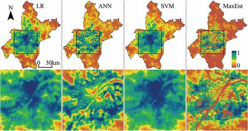
After training and testing the four models, they are used to project the TPMs of the three study areas. Figure 8, Figure 9, and Figure 10 show the TPMs of Beijing, Tianjin, and Wuhan, respectively. As can be seen from these figures, the TPMs predicted by the LR and SVM models are similar, but the SVM-TPMs of Tianjin and Wuhan have less high-potential cells, which indicates that the performance of the SVM training is slightly better. There is an obvious boundary between high-potential cells and low-potential cells in the ANN-TPMs and MaxEnt-TPMs, which means that the features of class differences between urban growth and non-urban growth have been learned by the ANN and MaxEnt training. However, the high-potential cells in the ANN-TPMs are concentrated and numerous, which may be due to the poor ability of the trained ANN models to determine the transition potential (Palani, Liong, and Tkalich 2008). Besides, to a certain extent, this also indicates that the ANN training is prone to over-fitting, which reduces its generalization ability (Paneiro et al. 2018). Compared with the TPMs predicted by LR, ANN, and SVM models, the MaxEnt-TPMs show more spatial details that characterize the influences of spatial factors on urban growth, especially the roads and water bodies. It can be seen from these figures that the MaxEnt-TPMs have relatively clear structures of road networks and clear contours of water bodies. High-potential cells are concentrated near road networks, while almost all the cells in the region of water bodies are low-potential cells. These characteristics indicate that the driving mechanisms of urban growth can be well learned by the MaxEnt training.

Figure 8. Transition potential maps of Beijing projected by LR, ANN, SVM, and MaxEnt models. The central zone of Beijing has been enlarged to show spatial details.

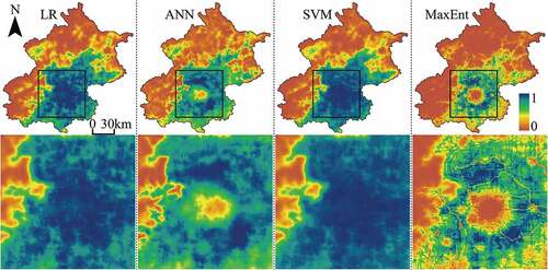
Figure 9. Transition potential maps of Tianjin projected by LR, ANN, SVM, and MaxEnt models. The central zone of Tianjin has been enlarged to show spatial details.

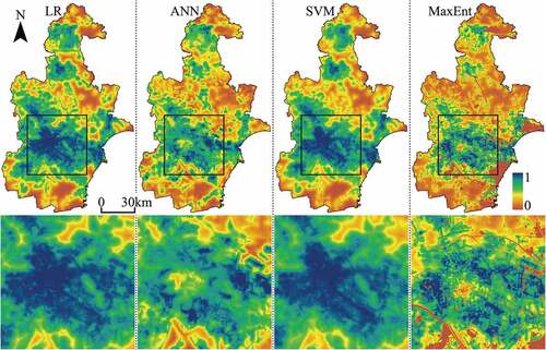
Figure 10. Transition potential maps of Wuhan projected by LR, ANN, SVM, and MaxEnt models. The central zone of Wuhan has been enlarged to show spatial details.

4.1.3 Time statistics

Table 3 shows the training and projecting time (without the time spent on importing the data of samples and spatial factors) for different methods in three study areas, on a computer with an AMD Ryzen 5 2600 × 3.60 GHz CPU, 16 GB memory, and Windows 10. Regardless of training or projecting, the time-consuming sequence of different methods is LR < ANN < MaxEnt < SVM. LR needs the least time for training and projecting, but it can only capture the linear characteristics of urban growth (Zhang and Xia 2021). ANN and SVM have advantages in capturing nonlinear characteristics of urban growth, but the computational efficiency of SVM is much lower than that of ANN, which may be due to their different modeling mechanisms. The data elements of ANN training are spatial variables, while the data elements of SVM training are individual samples, increasing the complexity of SVM training to mine sample information (Ding, Hua, and Yu 2014; Gundogdu et al. 2016). Therefore, the computational efficiency and the ability to handle large datasets of SVM are poor. The MaxEnt model incorporates feature engineering to improve its ability to capture complex characteristics of urban growth, and the methods of searching the optimal approximate distribution are essentially linear, which simplifies its training and improves the computational efficiency (Phillips, Anderson, and Schapire 2006; Phillips and Dudik 2008).

Table 3. The training and projecting time (second) for the LR, ANN, SVM, and MaxEnt models in Beijing, Tianjin, and Wuhan

Study area	Time\Method	LR	ANN	SVM	MaxEnt
Beijing	Training time	0.2780	3.2113	14.9110	13.1280
	Projecting time	0.3040	19.3607	5051.5970	156.4850
	Total time	0.5820	22.5720	5066.5970	169.6130
Tianjin	Training time	0.2160	3.1787	19.1640	13.0050
	Projecting time	0.2210	12.5205	4927.0870	120.4990
	Total time	0.4370	15.6992	4946.2510	133.5040
Wuhan	Training time	0.1760	4.6216	16.5870	13.0620
	Projecting time	0.2020	12.7564	2954.3230	101.3100
	Total time	0.3780	17.3780	2970.9100	114.3720

4.2 Comparison of the simulation performance of CA models

Four kinds of CA models, namely, LR-CA, ANN-CA, SVM-CA, and MaxEnt-CA models, are constructed to simulate the urban growth of Beijing, Tianjin, and Wuhan during 2000–2020, respectively. Referring to previous studies (Garcia et al. 2011, Feng et al. 2011; Li, Liu, and Yu 2014; Wu et al. 2019), the configurations of CA models are as follows. An extended Moore neighborhood with the size of 7 × 7 is used to characterize the local interactions of CA models. Existing urban land and water bodies are used as the ecological restraint of urban growth simulation, i.e. the state of cells in the region of existing urban land and water bodies cannot be changed in the simulation. The parameter that controls the degree of perturbation in the stochastic term is set to two. The time step of each iteration is set to half a year, i.e. there are 40 iterations in the simulation of urban growth during 2000–2020. It should be noted that each CA model has been run ten times to avoid noise, and the indicators mentioned below are the mean of ten replications.

4.2.1 Simulation results

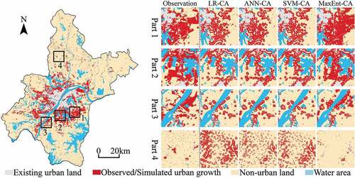
Figure 11, Figure 12 and Figure 13 respectively show the urban growth of Beijing, Tianjin and Wuhan, as well as the urban growth simulated by LR-CA, ANN-CA, SVM-CA, and MaxEnt-CA models. The advantages of the MaxEnt-CA model in simulating urban growth can be proved from two aspects, namely, the simulation of large-area urban growth (Part 1 and Part 2) and the simulation of sporadic urban growth (Part 3 and Part 4). For the simulation of large-area urban growth, the urban growth simulated by the MaxEnt-CA model is similar to the observation in quantity and morphology. However, the urban growth simulated by LR-CA, ANN-CA, and SVM-CA models is severely affected by existing urban land, which limits the simulated urban growth to the adjacent regions of existing urban land. This phenomenon may be due to the insufficient capability of LR, ANN, and SVM models to reveal driving mechanisms of spatial factors, making the neighborhood more influential than the transition rule in their CA simulations (Zhang and Wang 2021). For the simulation of sporadic urban growth, there are two cases: 1) the existing urban land is scattered and the newly urbanized patches are in different sizes and 2) the existing urban land is scattered and the newly urbanized patches are fragmented and in similar sizes. In terms of the former case (Part 3), the distribution characteristics of newly urbanized patches have been captured by the MaxEnt-CA model, while the urban growth simulated by the other CA models is still limited to the adjacent regions of existing urban land. For the latter case (Part 4), the urbanized cells simulated by LR-CA, ANN-CA, and SVM-CA models are much more than the observation, which significantly increases their error rates. Although the urban landscape simulated by the MaxEnt-CA model is not similar to the observation, the less quantity of newly urbanized cells has a significant effect on reducing simulation errors. All the above results indicate that the MaxEnt-CA model has a better performance in simulating urban growth.

Figure 11. The observed urban growth in Beijing from 2000 to 2020 and the urban growth simulated by LR-CA, ANN-CA, SVM-CA and MaxEnt-CA models.

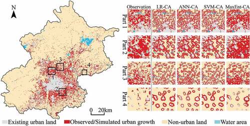
Figure 12. The observed urban growth in Tianjin from 2000 to 2020 and the urban growth simulated by LR-CA, ANN-CA, SVM-CA and MaxEnt-CA models.

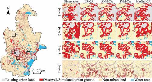
Figure 13. The observed urban growth in Wuhan from 2000 to 2020 and the urban growth simulated by LR-CA, ANN-CA, SVM-CA and MaxEnt-CA models.

4.2.2 Simulation accuracy

Table 4 shows the simulation accuracies of LR-CA, ANN-CA, SVM-CA, and MaxEnt-CA models in Beijing, Tianjin, and Wuhan. The simulation accuracy of the LR-CA model is used as the benchmark to show the performance promotion of the other CA models. As can be seen from the table, the simulation accuracy of the MaxEnt-CA model is the highest among the four kinds of CA models. Compared with the simulation accuracy of the LR-CA model, the simulation accuracy of the SVM-CA model slightly improves in Tianjin and Wuhan, and decreases in Beijing. The simulation accuracy of the ANN-CA model is higher than that of the LR-CA and SVM-CA models, but significantly lower than that of the MaxEnt-CA model, which indicates the accuracy advantage of the MaxEnt-CA model in simulating urban growth.

Table 4. The simulation accuracies of LR-CA, ANN-CA, SVM-CA, and MaxEnt-CA models in Beijing, Tianjin, and Wuhan

Study area	CA model	Kappa	Improvement (%)	FoM	Improvement (%)
Beijing	LR-CA	0.6903	–	0.3450	–
	ANN-CA	0.7070	1.67	0.3693	2.43
	SVM-CA	0.6870	−0.33	0.3404	−0.46
	MaxEnt-CA	0.7323	4.20	0.4076	6.26
Tianjin	LR-CA	0.6394	–	0.2418	–
	ANN-CA	0.6514	1.20	0.2577	1.59
	SVM-CA	0.6441	0.47	0.2480	0.62
	MaxEnt-CA	0.6732	3.38	0.2876	4.58
Wuhan	LR-CA	0.6786	–	0.3552	–
	ANN-CA	0.6972	1.86	0.3810	2.58
	SVM-CA	0.6878	0.92	0.3679	1.27
	MaxEnt-CA	0.7373	5.87	0.4401	8.49

4.2.3 Simulated urban landscape

Table 5 shows the landscape metrics of the urban landscape simulated by LR-CA, ANN-CA, SVM-CA, and MaxEnt-CA models in Beijing, Tianjin, and Wuhan. The LPIs of the simulation results of LR-CA, ANN-CA, SVM-CA models have different orders in the three study areas, but they are all lower than that of the MaxEnt-CA model. Similarly, the LSIs of the simulation results of the MaxEnt-CA model are the lowest among the four CA models, which is consistent in the three study areas. These results show that the aggregation degree of the urban landscape simulated by the MaxEnt-CA model is the highest among the involved CA models, while the shape complexity is the lowest, indicating the good performance of the MaxEnt-CA model in simulating regular urban landscape (Zhang et al. 2020b).

Table 5. The landscape metrics of the urban landscape simulated by LR-CA, ANN-CA, SVM-CA, and MaxEnt-CA models in Beijing, Tianjin, and Wuhan

Study area	Model	LPI	LSI
Beijing	LR-CA	0.0899	44.2720
	ANN-CA	0.0978	42.2888
	SVM-CA	0.0884	44.6563
	MaxEnt-CA	0.1296	36.9353
Tianjin	LR-CA	0.0805	50.0072
	ANN-CA	0.0694	51.7027
	SVM-CA	0.0829	49.7773
	MaxEnt-CA	0.0937	49.4785
Wuhan	LR-CA	0.0386	42.0907
	ANN-CA	0.0399	41.3345
	SVM-CA	0.0392	40.8573
	MaxEnt-CA	0.0613	33.3524

4.3 Driving mechanisms discovered by the MaxEnt modeling

4.3.1 Feature interpretation

Linear feature, quadratic feature, product feature, and hinge feature (including forward hinge feature and reverse hinge feature) are used to capture the complex characteristics of urban growth in the MaxEnt training. With normalized spatial variables, numerous features can be built through feature engineering, but only some significantly contributed features are selected to construct the MaxEnt model. Table 6 takes the Beijing as an example to show several instances of the selected features and corresponding parameters. All selected features and corresponding parameters for the MaxEnt modeling in the three study areas are shown in Table S1, Table S2, and Table S3, respectively. Lambda-value is the value of parameter λ in Equation (8)(8) $q_{\lambda }(x)=\frac{e^{\lambda \cdot f(x)}}{{\beta }_{\lambda }}$(8) for the corresponding feature (Elith et al. 2011). For linear, quadratic, and product features, Min and Max are the minimum and maximum values of the feature encountered during the training of the model; while for forward and reverse hinge features, Min and Max mean the interval of variable that needs to be linearly scaled (Merow, Smith, and Silander 2013).

Table 6. Partial selected features and corresponding parameters used in the MaxEnt modeling of the urban growth of Beijing. Labels of spatial variables are explained in Table 1

Feature type	Instance	Lambda-value	Min	Max
Linear	dis2CC	0	0.0086	0.9966
Quadratic	Eleva^2	0.4828	0.0051	0.9989
Product	dis2CC*dis2TRW	−1.8975	0.0009	0.9702
Forward hinge	‘dis2CC	0.5504	0.6852	0.9966
Reverse hinge	`dis2TRW	−0.2853	0.0397	0.4486

The lambda-value of the linear feature dis2CC is 0, which means that the relationship between variable dis2CC and urban growth is nonlinear (Elith et al. 2011; Merow, Smith, and Silander 2013). The quadratic feature Eleva^2 has a significant influence on modeling urban growth, and its lambda-value is 0.4828. The product feature dis2CC*dis2TRW means that there is an interaction between spatial variables dis2CC and dis2TRW, and the contribution of the interaction to modeling urban growth is significant with a lambda-value of −1.8975. The knot values of forward hinge feature ‘dis2CC and reverse hinge feature `dis2TRW are 0.6852 and 0.4486, respectively. It should be noted that, there may be many hinge features of the same variable with different knot values (see Table S1, Table S2, and Table S3), which allows the response to a variable to be modeled in a piece-wise fashion (Phillips and Dudik 2008).

4.3.2 Variable interactions

Table 7 shows the product features used in the MaxEnt modeling of urban growth of Beijing, Tianjin, and Wuhan, which represent the interactions between spatial variables. The number of interactions detected by the MaxEnt modeling somehow indicates the complexity of the driving mechanism of urban growth, with seven in Beijing, eleven in Tianjin, and four in Wuhan. Therefore, the sequence of complexity of the driving mechanisms in the three study areas is Tianjin > Beijing > Wuhan. This sequence can also be authenticated through comparing the simulation accuracies of CA models in different study areas, because the more complex the driving mechanisms, the more difficult to well simulate the urban growth. As can be seen from Table 4, no matter which kind of CA models is used, the sequence of simulation accuracies of the three study areas is Tianjin < Beijing < Wuhan, which can be the evidence of the above inference. Most of the variable interactions in the three study areas are related to traffic factors, which indicates that there is a strong correlation between traffic development and the urban growth of Beijing, Tianjin, and Wuhan.

Table 7. Product features used in the MaxEnt modeling of the urban growth of Beijing, Tianjin, and Wuhan. Labels of spatial variables are explained in Table 1

Study area	Product feature	Lambda-value	Min	Max
Beijing	dis2CC*dis2PRW	0.0089	0.0002	0.9864
	dis2CC*dis2RST	0.0190	0.0002	0.9895
	dis2CC*dis2TRW	−1.8975	0.0009	0.9702
	dis2DC*dis2TRW	0.1507	0.0069	0.9872
	dis2PRW*Slope	0.3711	0.0174	0.9975
	dis2RST*Eleva	0.7815	0.0040	0.9863
	dis2RST*Slope	0.3402	0.0066	0.9952
Tianjin	dis2CC*dis2DC	0.0099	0.0048	0.9517
	dis2CC*dis2TEW	0.3476	0.0079	0.9776
	dis2DC*dis2EEM	0.5271	0.0030	0.9489
	dis2DC*dis2TRW	0.1103	0.0289	0.9851
	dis2EEM*dis2RST	−0.1047	0.0166	0.9763
	dis2EEM*dis2TC	1.3685	0.0085	0.9744
	dis2PRW*dis2TRW	−0.9914	0.0228	0.9671
	dis2RST*dis2SEW	−0.2697	0.0446	0.9978
	dis2RST*dis2TRW	0.1302	0.0060	0.9938
	dis2TEW*dis2WAB	−1.8440	0.0105	0.9933
	dis2TEW*Eleva	0.0395	0.0532	0.9845
Wuhan	dis2DC*dis2EEM	−1.6721	0.0001	0.9071
	dis2DC*dis2TC	0.0864	0.0061	0.9800
	dis2EEM*dis2WAB	0.3513	0.0050	0.9908
	dis2RST*dis2TC	−1.6537	0.0046	0.9828

4.3.3 Response curves of spatial variables

The use of hinge feature allows the MaxEnt model to generate the response curves of spatial variables, which show the relationships between spatial variables and urban growth (Phillips and Dudik 2008). Figure 14, Figure 15, and Figure 16 show the response curves of spatial variables generated by the MaxEnt modeling of urban growth in Beijing, Tianjin, and Wuhan, respectively. All the relationships between spatial variables and urban growth are nonlinear, which can also be proved by the lambda-values of all linear features being 0 (see Table S1, Table S2, and Table S3). In Beijing and Wuhan, the transition potential generally increases with the normalized spatial variable value. However, there are inflection points in the response curves of spatial variables dis2CC, dis2DC, dis2RST, dis2EEM, dis2WAB, Eleva, and Slope. In other words, when the normalized value of such spatial variable is larger than the value of inflection point, the transition potential starts to decrease with the spatial variable value. This may be because that most of the proximate areas of some spatial factors such as city centers, district centers, railway and subway stations, entrances and exits of motorways, and water bodies are already urban land. Moreover, most of the areas with low elevation and slope are water bodies, which is especially common in Wuhan. Furthermore, there are some differences between the response curves of Tianjin and that of Beijing and Wuhan, especially the response curves of dis2CC and dis2WAB. This may be due to that Tianjin is a typical dual-core city and a port city, the coastal district named “Binhai New District” is the sub-core of Tianjin, which can be observed in Figure 2. Therefore, there is a trough in the response curves of dis2CC and dis2WAB. To a certain extent, it can be summarized that, the closer to spatial factors, the lower the elevation and slope, the higher the transition potential. Furthermore, the increase of transition potential is piecewise continuous, and the knot location of the response curve represents the radiation range affected by spatial factors (Wang et al. 2020).

Figure 14. The response curves showing the relationship between urban growth of Beijing and spatial variables dis2CC, dis2DC, dis2TC, dis2TRW, dis2PRW, dis2SEW, dis2TEW, dis2RST, dis2EEM, dis2WAB, Eleva, and Slope. Labels of spatial variables are explained in .Table 1

Figure 15. The response curves showing the relationship between urban growth of Tianjin and spatial variables dis2CC, dis2DC, dis2TC, dis2TRW, dis2PRW, dis2SEW, dis2TEW, dis2RST, dis2EEM, dis2WAB, Eleva, and Slope. Labels of spatial variables are explained in .Table 1

Figure 16. The response curves showing the relationship between urban growth of Wuhan and spatial variables dis2CC, dis2DC, dis2TC, dis2TRW, dis2PRW, dis2SEW, dis2TEW, dis2RST, dis2EEM, dis2WAB, Eleva, and Slope. Labels of spatial variables are explained in Table 1.

4.3.4 Importance of spatial variables

The importance of spatial variables can be obtained through analyzing the change of objective function value in the training iterations. In each iteration of the training algorithm, the increase of objective function value is added to the contribution of corresponding variable, or subtracted from it if the change to the absolute value of λ is negative (Merow, Smith, and Silander 2013). With this operation, the percent contributions of spatial variables can be obtained and shown in Table 8. Due to the special location of Beijing, topographic factors such as Eleva and Slope have significant effects on urban growth. As described in Section 2, Beijing adjoins the Taihang Mountains and locates in the north of the North China Plain. Therefore, there are obvious boundaries between different topographic areas of Beijing, which can be observed in the visualization of Eleva and Slope in Figure 3. Most of the existing and newly urbanized cells are located in the plain area, which amplifies the importance of topographic factors in the MaxEnt modeling. Besides, city center has significant effects on the urban growth of Beijing, which is due to that Beijing is a typical single-core city and city center is the radiation source of urban growth in the plain area. Tianjin, as a coastal port city, has small terrain changes and large water areas near the sea. Therefore, the effects of traffic factors and waterbodies on its urban growth are very significant. Furthermore, the dual-core structure of Tianjin city makes the effects of district centers more significant than that of the city center, which is different from Beijing and Wuhan. There are many water areas and hills in Wuhan (Lin et al. 2020), so the terrain of Wuhan is more complex than that of Beijing and Tianjin, which leads to a balanced driving mechanism, i.e. no spatial variable holds the absolute predominance in the MaxEnt modeling. Therefore, traffic factors, city center, and water bodies have important effects on the urban growth of Wuhan.

Table 8. The percent contributions of spatial variables in the MaxEnt modeling of the urban growth of Beijing, Tianjin, and Wuhan. Labels of spatial variables are explained in Table 1

Rank	Beijing		Tianjin		Wuhan
	Variable	Percent contribution	Variable	Percent contribution	Variable	Percent contribution
1	Eleva	34.6	dis2TEW	36.1	dis2TEW	23.4
2	Slope	25.8	dis2RST	16.9	dis2CC	20.9
3	dis2CC	14.3	dis2WAB	14.9	dis2RST	14.6
4	dis2TEW	7.1	dis2DC	9.3	dis2WAB	11.6
5	dis2PRW	3.3	dis2CC	5.2	dis2PRW	8.8
6	dis2WAB	3.3	dis2PRW	4.1	dis2TRW	7.9
7	dis2SEW	2.8	Eleva	4.0	dis2SEW	6.2
8	dis2DC	2.5	dis2SEW	3.5	dis2DC	3.2
9	dis2TC	2.5	dis2TC	2.2	dis2EEM	2.2
10	dis2RST	1.9	dis2TRW	2.2	Eleva	1.0
11	dis2TRW	1	dis2EEM	1.1	Slope	0.1
12	dis2EEM	0.9	Slope	0.5	dis2TC	0.1

5 Discussion

In recent years, the MaxEnt model has been widely used in geographic modeling, and various studies have proved its powerful ability to predict unknown distributions based on known information (Phillips, Anderson, and Schapire 2006; Galletti et al. 2013; Merow, Smith, and Silander 2013). In the field of CA simulation, Zhang et al. (2020b) incorporated the MaxEnt model and the CA model to simulate the land use/cover change (LUCC) of China; and Wang et al. (2020) adopted the MaxEnt model to optimize the stochastic component of CA model for urban growth simulation. Although they stated that good results had been obtained by incorporating the MaxEnt model, they did not explore the advantages of the MaxEnt model over other approaches such as LR, ANN, and SVM models, which may impede the wide application of the MaxEnt model in CA-based simulation of urban growth.

The advantages of a CA modeling method are often investigated by comparing the simulation performance of CA models. However, this kind of evaluation is biased, because it is no longer difficult to improve the simulation accuracy of CA models with the development of machine learning. Many machine learning algorithms and their derivatives can be used to calibrate CA models and obtain excellent simulation accuracy (Li and Gong 2016). Yet, most of these algorithms such as ANN and SVM are black-box methods, which can not explicitly interpret the driving mechanisms of urban growth (Phillips et al. 2015). Moreover, using the CA model to simulate urban growth is not to seek simulation results with high accuracy, but to understand and predict the urban growth process and reveal its hidden mechanisms (Tobler 1970; Aburas et al. 2016; Li et al. 2017; Liang et al. 2018). Therefore, to evaluate the advantages of a CA modeling method, two aspects should be included, i.e. the simulation performance and the ability to interpret driving mechanisms.

In this study, four methods including LR, ANN, SVM, and MaxEnt are compared to highlight the advantages of the MaxEnt model in calibrating CA for urban growth simulation. The training and testing accuracy of the MaxEnt model is second only to that of the ANN model, but its projecting accuracy is the highest. This is because the ANN model has an excellent ability in learning the features of class differences, but has a poor ability to determine the transition potential based on spatial variables, which may be due to its inferior generalization ability caused by over-fitting (Palani, Liong, and Tkalich 2008; Paneiro et al. 2018). Therefore, it can be considered that the performance of the MaxEnt (or MaxEnt-CA) is better than the other methods except for the computational efficiency. Although the computational efficiency of the MaxEnt model is not the best, the time it requires for training and projecting is also acceptable. In short, compared with LR, ANN and SVM models, the MaxEnt model outperforms them in calibrating CA for urban growth simulation.

The ability to interpret driving mechanisms is also an important aspect to judge the advantages of a CA modeling method. ANN and SVM are both black-box models that cannot offer explicit interpretations of driving mechanisms. Although LR can explicitly obtain the weights of spatial variables (Table S4) and interpret driving mechanisms, it can only characterize the linear features of urban growth and has no ability to describe nonlinear and complex urban dynamics. Furthermore, the interactions between spatial variables are not considered in the training of LR, ANN, and SVM models, which are important for interpreting driving mechanisms. By contrast, the interactions, response curves, and importance of spatial variables are considered in the MaxEnt training and can be explicitly interpreted (Phillips, Anderson, and Schapire 2006; Phillips and Dudik 2008). Moreover, the incorporation of feature engineering improves its ability to capture complex and nonlinear characteristics of urban growth. These incorporations together with their explicit interpretations determine the advantages of the MaxEnt model in interpreting the driving mechanisms of urban growth.

6 Conclusion

This paper compares and analyzes four methods to calibrate CA models for urban growth simulation, namely, LR, ANN, SVM, and MaxEnt models. The advantages of the MaxEnt model over other models have been proved and interpreted. The LR-CA, ANN-CA, SVM-CA, and MaxEnt-CA models are successfully conducted to simulate the urban growth of Beijing, Tianjin, and Wuhan during 2000–2020. The comparison is carried out from several aspects, including the accuracy of training, testing, and projected TPMs, computational efficiency, simulation accuracy, simulated urban landscape, and the ability to discover and interpret driving mechanisms of urban growth. The results indicate that the MaxEnt model is superior to the other models in all the aspects except for the computational efficiency, but the time required for the training and projecting of the MaxEnt model is acceptable and far less than that of SVM.

However, there are also some limitations in this study. First, the performance of the four models has only been investigated in the calibration of CA models, and their generalization ability in urban growth prediction needs more exploration. Second, sample size and sample prevalence may have significant influences on the performance of the four models, which should be tested in further research. Finally, future research can apply the four methods into other regions to further verify the findings of this study.

Highlights

The advantages of the MaxEnt model in calibrating CA models have been explored.

The performance of CA models calibrated by LR, ANN, SVM, and MaxEnt was compared.

MaxEnt-CA model has the best simulation performance among the involved CA models.

Driving mechanisms of urban growth were explicitly interpreted by MaxEnt modelling.

Data and codes availability statement

The data and codes that support the findings of this study are openly available at [10.6084/m9.figshare.14716974.v1].

Acknowledgements

We thank the anonymous reviewers and journal editors for their constructive comments and suggestions that greatly improved the article. This work is supported by the National Natural Science Foundation of China (42171411).

Disclosure statement

No potential conflict of interest was reported by the author(s).

Additional information

Funding

This work was supported by the National Natural Science Foundation of China [42171411].

References

- Aburas, M. M., Y. M. Ho, M. F. Ramli, and Z. H. Ash’aari. 2016. “The Simulation and Prediction of Spatio-temporal Urban Growth Trends Using Cellular Automata Models: A Review.” International Journal of Applied Earth Observation and Geoinformation 52: 380–389. doi:10.1016/j.jag.2016.07.007.
- Beijing Municipal Bureau Statistics & Survey Office of the National Bureau of Statistics in Beijing. 2020. Beijing Statistical Yearbook 2020. Bejing: China Statistics Press. http://nj.tjj.beijing.gov.cn/nj/main/2020-tjnj/zk/indexch.htm
- Berberoglu, S., A. Akin, and K. C. Clarke. 2016. “Cellular Automata Modeling Approaches to Forecast Urban Growth for Adana, Turkey: A Comparative Approach.” Landscape and Urban Planning 153: 11–27. doi:10.1016/j.landurbplan.2016.04.017.
- Chang, C. C., and C. J. Lin. 2011. “LIBSVM: A Library for Support Vector Machines.” ACM Transactions on Intelligent Systems and Technology 2 (3): 1–39. doi:10.1145/1961189.1961199.
- Chen, J., L. J. Chen, F. Chen, Y. F. , et al. 2021. “Collaborative Validation of GlobeLand30: Methodology and Practices.” Geo-Spatial Information Science 24 (1): 134–144. doi:10.1080/10095020.2021.1894906.
- Chettry, V., and M. Surawar. 2021. “Urban Sprawl Assessment in Eight Mid-sized Indian Cities Using RS and GIS.” Journal of the Indian Society of Remote Sensing. doi:10.1007/s12524-021-01420-8.
- Dahal, K. R., and T. E. Chow. 2015. “Characterization of Neighborhood Sensitivity of an Irregular Cellular Automata Model of Urban Growth.” International Journal of Geographical Information Science 29 (3): 475–497. doi:10.1080/13658816.2014.987779.
- DellaPietra, S., V. DellaPietra, and J. Lafferty. 1997. “Inducing Features of Random Fields.” IEEE Transactions on Pattern Analysis and Machine Intelligence 19 (4): 380–393. doi:10.1109/34.588021.
- Ding, S. F., X. P. Hua, and J. Z. Yu. 2014. “An Overview on Nonparallel Hyperplane Support Vector Machine Algorithms.” Neural Computing & Applications 25 (5): 975–982. doi:10.1007/s00521-013-1524-6.
- Du, G. D., et al. 2018. “A Comparative Approach to Modelling Multiple Urban Land Use Changes Using Tree-based Methods and Cellular Automata: The Case of Greater Tokyo Area.” International Journal of Geographical Information Science 32 (4): 757–782. doi:10.1080/13658816.2017.1410550.
- Dudík, M., S. J. Phillips, and R. E. Schapire (2004). “Performance Guarantees for Regularized Maximum Entropy Density Estimation.” In: Proceedings of the 17th Annual Conference on Computational Learning Theory, ACM Press, New York, pp. 655–662.
- Elith, J., S. J. Phillips, T. Hastie, et al. 2011. “A Statistical Explanation of MaxEnt for Ecologists.” Diversity & Distributions 17 (1): 43–57. doi:10.1111/j.1472-4642.2010.00725.x.
- Feng, Y. J., Y. Liu, X. H. Tong, et al. 2011. “Modelling Dynamic Urban Growth Using Cellular Automata and Particle Swarm Optimization Rules.” Landscape and Urban Planning 102 (3): 188–196. doi:10.1016/j.landurbplan.2011.04.004.
- Feng, Y. J., Y. Liu, and X. H. Tong. 2018. “Comparison of Metaheuristic Cellular Automata Models: A Case Study of Dynamic Land Use Simulation in the Yangtze River Delta.” Computers, Environment and Urban Systems 70: 138–150. doi:10.1016/j.compenvurbsys.2018.03.003.
- Fik, T. J., D. C. Ling, and G. F. Mulligan. 2003. “Modelling Spatial Variation in Housing Prices: A Variable Interaction Approach.” Real Estate Economics 31 (4): 623–646. doi:10.1046/j.1080-8620.2003.00079.x.
- Galletti, C. S., E. Ridder, S. E. Falconer, and P. L. Fall. 2013. “Maxent Modelling of Ancient and Modern Agricultural Terraces in the Troodos Foothills, Cyprus.” Applied Geography 39: 46–56. doi:10.1016/j.apgeog.2012.11.020.
- Gao, C., Y. J. Feng, X. H. Tong, et al. 2020. “Modeling Urban Growth Using Spatially Heterogeneous Cellular Automata Models: Comparison of Spatial Lag, Spatial Error and GWR.” Computers, Environment and Urban Systems 81:101459. doi:10.1016/j.compenvurbsys.2020.101459.
- Garcia, A. M., I. Sante, M. Boullon, and R. Crecente. 2013. “Calibration of an Urban Cellular Automaton Model by Using Statistical Techniques and a Genetic Algorithm. Application to a Small Urban Settlement of NW Spain.” International Journal of Geographical Information Science 27 (8): 1593–1611. doi:10.1080/13658816.2012.762454.
- Garcia, A. M., I. Sante, R. Crecente, and D. Miranda. 2011. “An Analysis of the Effect of the Stochastic Component of Urban Cellular Automata Models.” Computers, Environment and Urban Systems 35 (4): 289–296. doi:10.1016/j.compenvurbsys.2010.11.001.
- Gundogdu, O., E. Egrioglu, C. H. Aladag, and U. Yolcu. 2016. “Multiplicative Neuron Model Artificial Neural Network Based on Gaussian Activation Function.” Neural Computing & Applications 27 (4): 927–935. doi:10.1007/s00521-015-1908-x.
- Huang, B., et al. 2009. “Land-use-change Modelling Using Unbalanced Support-vector Machines.” Environment and Planning B-Planning & Design 36 (3): 398–416. doi:10.1068/b33047.
- Jaynes, E. T. 1957. “Information Theory and Statistical Mechanics.” Physical Review 106 (4): 620–630. doi:10.1103/PhysRev.106.620.
- Jaynes, E. T. 1982. “On the Rationale of Maximum-Entropy Method.” Proceedings of the IEEE 70 (9): 939–952. doi:10.1109/PROC.1982.12425.
- Kamusoko, C., and J. Gamba. 2015. “Simulating Urban Growth Using a Random Forest-Cellular Automata (RF-CA) Model.” ISPRS International Journal of Geo-Information 4 (2): 447–470. doi:10.3390/ijgi4020447.
- Karimi, F., et al. 2019. “An Enhanced Support Vector Machine Model for Urban Expansion Prediction.” Computers, Environment and Urban Systems 75:61–75. doi:10.1016/j.compenvurbsys.2019.01.001.
- Kenny, D. A., and C. M. Judd. 1984. “Estimating the Nonlinear and Interactive Effects of Latent Variables.” Psychological Bulletin 96 (1): 201–210. doi:10.1037/0033-2909.96.1.201.
- Kocabas, V., and S. Dragicevic. 2006. “Assessing Cellular Automata Model Behaviour Using a Sensitivity Analysis Approach.” Computers, Environment and Urban Systems 30 (6): 921–953. doi:10.1016/j.compenvurbsys.2006.01.001.
- Kocabas, V., and S. Dragicevic. 2007. “Enhancing a GIS Cellular Automata Model of Land Use Change: Bayesian Networks, Influence Diagrams and Causality.” Transactions in GIS 11 (5): 681–702. doi:10.1111/j.1467-9671.2007.01066.x.
- Li, X. C., and P. Gong. 2016. “Urban Growth Models: Progress and Perspective.” Science Bulletin 61 (21): 1637–1650. doi:10.1007/s11434-016-1111-1.
- Li, X. C., X. P. Liu, and L. Yu. 2014. “A Systematic Sensitivity Analysis of Constrained Cellular Automata Model for Urban Growth Simulation Based on Different Transition Rules.” International Journal of Geographical Information Science 28 (7): 1317–1335. doi:10.1080/13658816.2014.883079.
- Li, X., C. H. Lao, X. P. Liu, and Y. M. Chen. 2011. “Coupling Urban Cellular Automata with Ant Colony Optimization for Zoning Protected Natural Areas under a Changing Landscape.” International Journal of Geographical Information Science 25 (4): 575–593. doi:10.1080/13658816.2010.481262.
- Li, X., Y. M. Chen, X. P. Liu, X. C. Xu, and G. L. Chen. 2017. “Experiences and Issues of Using Cellular Automata for Assisting Urban and Regional Planning in China.” International Journal of Geographical Information Science 31 (8): 1606–1629. doi:10.1080/13658816.2017.1301457.
- Liang, X., X. P. Liu, D. Li, H. Zhao, and G. Z. Chen. 2018. “Urban Growth Simulation by Incorporating Planning Policies into a CA-based Future Land-use Simulation Model.” International Journal of Geographical Information Science 32 (11): 2294–2316. doi:10.1080/13658816.2018.1502441.
- Liao, J. F., L. N. Tang, G. F. Shao, Q. Y. Qiu, C. P. Wang, S. N. Zheng, and X. D. Su. 2014. “A Neighbor Decay Cellular Automata Approach for Simulating Urban Expansion Based on Particle Swarm Intelligence.” International Journal of Geographical Information Science 28 (4): 720–738. doi:10.1080/13658816.2013.869820.
- Lin, A. Q., H. Wu, G. H. Liang, et al. 2020. “A Big Data-driven Dynamic Estimation Model of Relief Supplies Demand in Urban Flood Disaster.” International Journal of Disaster Risk Reduction 49:101682. doi:10.1016/j.ijdrr.2020.101682.
- McGarigal, K., S. A. Cushman, and E. Ene. 2012. “FRAGSTATS V4: Spatial Pattern Analysis Program for Categorical and Continuous Maps.” Computer software program produced by the authors at the University of Massachusetts, Amherst. http://www.umass.edu/landeco/research/fragstats/fragstats.html
- Merow, C., M. J. Smith, and J. A. Silander. 2013. “A Practical Guide to MaxEnt for Modelling Species’ Distributions: What It Does, and Why Inputs and Settings Matter.” Ecography 36 (10): 1058–1069. doi:10.1111/j.1600-0587.2013.07872.x.
- Mohammad-Djafari, A. 2015. “Entropy, Information Theory, Information Geometry and Bayesian Inference in Data, Signal and Image Processing and Inverse Problems.” Entropy 17 (6): 3989–4027. doi:10.3390/e17063989.
- Müller, K., C. Steinmeier, and M. Küchler. 2010. “Urban Growth along Motorways in Switzerland.” Landscape and Urban Planning 98 (1): 3–12. doi:10.1016/j.landurbplan.2010.07.004.
- Munshi, T., M. Zuidgeest, M. Brussel, and M. van Maarseveen. 2014. “Logistic Regression and Cellular Automata-based Modelling of Retail, Commercial and Residential Development in the City of Ahmedabad, India.” Cities 39: 68–86. doi:10.1016/j.cities.2014.02.007.
- Mustafa, A., A. Rienow, I. Saadi, et al. 2018. “Comparing Support Vector Machines with Logistic Regression for Calibrating Cellular Automata Land Use Change Models.” European Journal of Remote Sensing 51 (1): 391–401. doi:10.1080/22797254.2018.1442179.
- Omrani, H., A. Tayyebi, and B. Pijanowski. 2017. “Integrating the Multi-label Land-use Concept and Cellular Automata with the Artificial Neural Network-based Land Transformation Model: An Integrated ML-CA-LTM Modelling Framework.” Giscience & Remote Sensing 54 (3): 283–304. doi:10.1080/15481603.2016.1265706.
- Palani, S., S. Y. Liong, and P. Tkalich. 2008. “An ANN Application for Water Quality Forecasting.” Marine Pollution Bulletin 56 (9): 1586–1597. doi:10.1016/j.marpolbul.2008.05.021.
- Paneiro, G., F. O. Durao, M. C. E. Silva, and P. F. Neves. 2018. “Artificial Neural Network Model for Ground Vibration Amplitudes Prediction Due to Light Railway Traffic in Urban Areas.” Neural Computing & Applications 29 (11): 1045–1057. doi:10.1007/s00521-016-2625-9.
- Park, S., S. Jeon, and C. Choi. 2012. “Mapping Urban Growth Probability in South Korea: Comparison of Frequency Ratio, Analytic Hierarchy Process, and Logistic Regression Models and Use of the Environmental Conservation Value Assessment.” Landscape and Ecological Engineering 8 (1): 17–31. doi:10.1007/s11355-010-0137-9.
- Phillips, J., E. Cripps, J. W. Lau, and M. R. Hodkiewicz. 2015. “Classifying Machinery Condition Using Oil Samples and Binary Logistic Regression.” Mechanical Systems and Signal Processing 60-61: 316–325. doi:10.1016/j.ymssp.2014.12.020.
- Phillips, S. J., and M. Dudik. 2008. “Modelling of Species Distributions with Maxent: New Extensions and a Comprehensive Evaluation.” Ecography 31 (2): 161–175. doi:10.1111/j.0906-7590.2008.5203.x.
- Phillips, S. J., R. P. Anderson, and R. E. Schapire. 2006. “Maximum Entropy Modelling of Species Geographic Distributions.” Ecological Modelling 190 (3–4): 231–259. doi:10.1016/j.ecolmodel.2005.03.026.
- Pontius, R. G., W. Boersma, J. C. Castella, et al. 2008. “Comparing the Input, Output, and Validation Maps for Several Models of Land Change.” Annals of Regional Science 42 (1): 11–37. doi:10.1007/s00168-007-0138-2.
- Prakash, J., S. Mandal, D. Razansky, and V. Ntziachristos. 2018. “Maximum Entropy Based Non-negative Optoacoustic Tomographic Image Reconstruction.” IEEE Transactions on Biomedical Engineering 66 (9): 2604–2616. doi:10.1109/TBME.2019.2892842.
- Rao, R. K., K. Tun, and S. Lakshminarayanan. 2009. “Genetic Programming Based Variable Interaction Models for Classification of Process and Biological Systems.” Industrial & Engineering Chemistry Research 48 (10): 4899–4907. doi:10.1021/ie801147m.
- Rienow, A., and R. Goetzke. 2015. “Supporting SLEUTH-Enhancing a Cellular Automaton with Support Vector Machines for Urban Growth Modelling.” Computers, Environment and Urban Systems 49: 66–81. doi:10.1016/j.compenvurbsys.2014.05.001.
- Roodposhti, M. S., J. Aryal, and B. A. Bryan. 2019. “A Novel Algorithm for Calculating Transition Potential in Cellular Automata Models of Land-use/cover Change.” Environmental Modelling and Software 112: 70–81. doi:10.1016/j.envsoft.2018.10.006.
- Sante, I., A. M. Garcia, D. Miranda, and R. Crecente. 2010. “Cellular Automata Models for the Simulation of Real-world Urban Processes: A Review and Analysis.” Landscape and Urban Planning 96 (2): 108–122. doi:10.1016/j.landurbplan.2010.03.001.
- Shafizadeh-Moghadam, H., et al. 2017a. “Sensitivity Analysis and Accuracy Assessment of the Land Transformation Model Using Cellular Automata.” GIScience & Remote Sensing 54 (5): 639–656. doi:10.1080/15481603.2017.1309125.
- Shafizadeh-Moghadam, H., et al. 2017b. “Coupling Machine Learning, Tree-based and Statistical Models with Cellular Automata to Simulate Urban Growth.” Computers, Environment and Urban Systems 64:297–308. doi:10.1016/j.compenvurbsys.2017.04.002.
- Shafizadeh-Moghadam, H., et al. 2021. “Integrating a Forward Feature Selection Algorithm, Random Forest, and Cellular Automata to Extrapolate Urban Growth in the Tehran-Karaj Region of Iran.” Computers, Environment and Urban Systems 87:101595. doi:10.1016/j.compenvurbsys.2021.101595.
- Shannon, C. E. 1948. “A Mathematical Theory of Communication.” Bell System Technical Journal 27 (3): 379–423. doi:10.1002/j.1538-7305.1948.tb01338.x.
- Shen, X. J., L. Mu, Z. Li, et al. 2016. “Large-scale Support Vector Machine Classification with Redundant Data Reduction.” Neurocomputing 172:189–197. doi:10.1016/j.neucom.2014.10.102.
- Stevens, D., S. Dragicevic, and K. Rothley. 2007. “iCity: A GIS-CA Modelling Tool for Urban Planning and Decision Making.” Environmental Modelling and Software 22 (6): 761–773. doi:10.1016/j.envsoft.2006.02.004.
- Tianjin Municipal Bureau Statistics & Survey Office of the National Bureau of Statistics in Tianjin. 2020. Tianjin Statistical Yearbook 2020. Bejing: China Statistics Press. http://stats.tj.gov.cn/nianjian/2020nj/zk/indexch.htm
- Tobler, W. R. 1970. “A Computer Movie Simulating Urban Growth in the Detroit Region.” Economic Geography 46 (sup1): 234–240. doi:10.2307/143141.
- Tobler, W. R. 1979. “Cellular Geography.” In Philosophy in Geography, edited by S. Gale, G. Olsson, and D. Dordrechet, 279–386. Reidel . doi:10.1007/978-94-009-9394-5_18.
- Tong, X. H., and Y. J. Feng. 2020. “A Review of Assessment Methods for Cellular Automata Models of Land-use Change and Urban Growth.” International Journal of Geographical Information Science 34 (5): 866–898. doi:10.1080/13658816.2019.1684499.
- Venkatraman, E. S. 2000. “A Permutation Test to Compare Receiver Operating Characteristic Curves.” Biometrics 56 (4): 1134–1138. doi:10.1111/j.0006-341X.2000.01134.x.
- Vermeiren, K., A. Van Rompaey, M. Loopmans, E. Serwajja, and P. Mukwaya. 2012. “Urban Growth of Kampala, Uganda: Pattern Analysis and Scenario Development.” Landscape and Urban Planning 106 (2): 199–206. doi:10.1016/j.landurbplan.2012.03.006.
- Wang, H. J., B. Zhang, C. Xia, S. W. He, and W. T. Zhang. 2020. “Using a Maximum Entropy Model to Optimize the Stochastic Component of Urban Cellular Automata Models.” International Journal of Geographical Information Science 34 (5): 924–946. doi:10.1080/13658816.2019.1687898.
- Wang, Q., T. T. Nguyen, J. Z. Huang, and T. T. Nguyen. 2018. “An Efficient Random Forests Algorithm for High Dimensional Data Classification.” Advances in Data Analysis and Classification 12 (4): 953–972. doi:10.1007/s11634-018-0318-1.
- Wang, W. L., L. M. Jiao, Q. Q. Jia, et al. 2021. “Land Use Optimization Modelling with Ecological Priority Perspective for Large-scale Spatial Planning.” Sustainable Cities and Society 65:102575. doi:10.1016/j.scs.2020.102575.
- White, R., and G. Engelen. 1993. “Cellular Automata and Fractal Urban Form: A Cellular Modelling Approach to the Evolution of Urban Land-use Patterns.” Environment and Planning A-Economy and Space 25 (8): 1175–1199. doi:10.1068/a251175.
- Wilson, A. 2010. “Entropy in Urban and Regional Modelling: Retrospect and Prospect.” Geographical Analysis 42 (4): 364–394. doi:10.4324/9780203142608.
- Wright, M. N., A. Ziegler, and I. R. Konig. 2016. “Do Little Interactions Get Lost in Dark Random Forests?” BMC Bioinformatics 17: 145. doi:10.1186/s12859-016-0995-8.
- Wu, F. L. 2002. “Calibration of Stochastic Cellular Automata: The Application to Rural-urban Land Conversions.” International Journal of Geographical Information Science 16 (8): 795–818. doi:10.1080/13658810210157769.
- Wu, H., A. Q. Lin, X. D. Xing, et al. 2021. “Identifying Core Driving Factors of Urban Land Use Change from Global Land Cover Products and POI Data Using the Random Forest Method.” International Journal of Applied Earth Observation and Geoinformation 103:102475. doi:10.1016/j.jag.2021.102475.
- Wu, H., Z. Li, K. C. Clarke, et al. 2019. “Examining the Sensitivity of Spatial Scale in Cellular Automata Markov Chain Simulation of Land Use Change.” International Journal of Geographical Information Science 33 (5): 1040–1061. doi:10.1080/13658816.2019.1568441.
- Wuhan Municipal Statistics Bureau & State Statistical Bureau Wuhan Investigation Team. 2020. Wuhan Statistical Yearbook 2020. Beijing: China Statistics Press. http://tjj.wuhan.gov.cn/tjfw/tjnj/202102/t20210202_1624450.shtml
- Xia, C., and B. Zhang. 2021. “Exploring the Effects of Partitioned Transition Rules upon Urban Growth Simulation in a Megacity Region: A Comparative Study of Cellular Automata-based Models in the Greater Wuhan Area.” GIScience & Remote Sensing 58 (5): 693–716. doi:10.1080/15481603.2021.1933714.
- Xu, T. T., J. Gao, and G. Coco. 2019. “Simulation of Urban Expansion via Integrating Artificial Neural Network with Markov Chain-cellular Automata.” International Journal of Geographical Information Science 33 (10): 1960–1983. doi:10.1080/13658816.2019.1600701.
- Yu, J., Y. Chen, J. P. Wu, and S. Khan. 2011. “Cellular Automata-based Spatial Multi-criteria Land Suitability Simulation for Irrigated Agriculture.” International Journal of Geographical Information Science 25 (1): 131–148. doi:10.1080/13658811003785571.
- Zhang, B., and C. Xia. 2021. “The Effects of Sample Size and Sample Prevalence on Cellular Automata Simulation of Urban Growth.” International Journal of Geographical Information Science 36 (1): 158–187. doi:10.1080/13658816.2021.1931237.
- Zhang, B., and H. J. Wang. 2021. “A New Type of Dual-scale Neighborhood Based on Vectorization for Cellular Automata Models.” GIScience & Remote Sensing 58 (3): 386–404. doi:10.1080/15481603.2021.1883946.
- Zhang, B., H. J. Wang, S. W. He, and C. Xia. 2020a. “Analyzing the Effects of Stochastic Perturbation and Fuzzy Distance Transformation on Wuhan Urban Growth Simulation.” Transactions in GIS 24 (6): 1779–1798. doi:10.1111/tgis.12683.
- Zhang, Y. H., X. P. Liu, G. L. Chen, and G. H. Hu. 2020b. “Simulation of Urban Expansion Based on Cellular Automata and Maximum Entropy Model.” Science China Earth Sciences 63 (5): 701–712. doi:10.1007/s11430-019-9530-8.
- Zhao, G., B. Pang, Z. X. Xu, et al. 2019. “Assessment of Urban Flood Susceptibility Using Semi-supervised Machine Learning Model.” Science of the Total Environment 659:940–949. doi:10.1016/j.scitotenv.2018.12.217.