A stacking ensemble algorithm for improving the biases of forest aboveground biomass estimations from multiple remotely sensed datasets

ABSTRACT

Accurately quantifying the aboveground biomass (AGB) of forests is crucial for understanding global change-related issues such as the carbon cycle and climate change. Many studies have estimated AGB from multiple remotely sensed datasets using various algorithms, but substantial uncertainties remain in AGB predictions. In this study, we aim to explore whether diverse algorithms stacked together are able to improve the accuracy of AGB estimates. To build the stacking framework, five base learners were first selected from a series of algorithms, including multivariate adaptive regression splines (MARS), support vector regression (SVR), multilayer perceptron (MLP) model, random forests (RF), extremely randomized trees (ERT), stochastic gradient boosting (SGB), gradient-boosted regression tree (GBRT) algorithm, and categorical boosting (CatBoost), based on diversity and accuracy metrics. Ridge and RF were utilized as the meta learner to combine the outputs of base learners. In addition, six important features were selected according to the feature importance values provided by the CatBoost, ERT, GBRT, SGB, MARS and RF algorithms as inputs of the meta learner in the stacking process. We then used stacking models with 3–5 selected base learners and ridge or RF to estimate AGB. The AGB data compiled from plot-level forest AGB, high-resolution AGB data derived from field and lidar data and the corresponding predictor variables extracted from the satellite-derived leaf area index, net primary production, forest canopy height, tree cover data, and Global Multiresolution Terrain Elevation Data 2010, as well as climate data, were randomly split into groups of 80% for training the model and 20% for model evaluation. The evaluation results showed that stacking generally outweighed the optimal base learner and provided improved AGB estimations, mainly by decreasing the bias. All stacking models had relative improvement (RI) values in bias of at least 22.12%, even reaching more than 90% under some scenarios, except for deciduous broadleaf forests, where an optimal algorithm could provide low biased estimations. In contrast, the improvements of stacking in R² and RMSE were not significant. The stacking of MARS, MLP, and SVR provided improved results compared with the optimal base learner, and the average RI in R² was 3.54% when we used all data without separating forest types. Finally, the optimal stacking model was used to generate global forest AGB maps.

KEYWORDS:

• Stacking
• forest biomass
• ensemble algorithm
• remote sensing

1. Introduction

Accurately quantifying the aboveground biomass (AGB) of forests is crucial for understanding global change-related issues, such as the carbon cycle and climate change (Houghton, Hall, and Goetz 2009). In recent decades, many studies have estimated forest AGB from optical images, synthetic aperture radar (SAR), and light detection and ranging (LiDAR) data at local or regional scales (Lu et al. 2016; Zolkos, Goetz, and Dubayah 2013; Wulder et al. 2012; Neumann et al. 2012). However, large uncertainties remain in existing forest AGB maps (Saatchi et al. 2011; Baccini et al. 2012; Mitchard et al. 2013).

To improve the accuracy of AGB predictions, recent efforts have concentrated on building ground-based forest observation systems (Chave et al. 2019) and providing new remotely sensed data sources, such as the Global Ecosystem Dynamics Investigation LiDAR and the European Space Agency P-band radar (Carreiras et al. 2017; Qi et al. 2019), and the integration of multisource remotely sensed data (Zhang and Liang 2020; Luo et al. 2019; Kattenborn et al. 2015). In addition, data-driven machine learning algorithms have been developed, along with an increasing number of remote sensing observations, and their performance in estimating AGB has been explored (Gleason and Im 2012; López-Serrano et al. 2016; de Almeida et al. 2019). However, each algorithm has its own scope of application, and no algorithm has good performance in all situations (Wang, Wu, and Mo 2013). There is on the pursuit for the most robust algorithms which are appropriate for forest AGB estimation or mapping, particularly at large scales.

Rather than selecting the single best model to estimate land surface parameters from remotely sensed data, ensemble algorithms combine the advantages of multiple learners, leading to an improved prediction accuracy (Zhang et al. 2020; Mendes-Moreira et al. 2012). Currently, ensemble algorithms used for estimating forest AGB are mainly homogeneous ensemble algorithms that aggregate results from the same algorithm, such as tree-based bagging represented by random forests (RF) and boosting represented by stochastic gradient boosting (SGB), gradient-boosted regression tree (GBRT) algorithms, categorical boosting (CatBoost), and extreme gradient boosting (XGBoost) regression algorithms (Breiman 2001; Belgiu and Drăguţ 2016; Friedman 2001, 2002; Huang et al. 2019). Bagging generates bootstrap samples from the original datasets to train weak decision tree models and then averages the outputs to obtain final predictions, which reduces the prediction variance (Yang et al. 2010), whereas boosting converts weak learners to strong learners by increasing the weights of samples with higher prediction errors in the following iteration, thereby gradually improving the prediction accuracy by decreasing the bias (Bühlmann and Hothorn 2007). It has been widely demonstrated that a series of bagging and boosting algorithms outperformed individual learning algorithms in estimating forest AGB (Zhang et al. 2020; Li et al. 2020). However, heterogeneous ensemble algorithms, which can combine diverse learners, including both individual algorithms and homogeneous ensemble algorithms mentioned above, thus providing better prediction results (Healey et al. 2018; Naimi and Balzer 2018), are still in its infancy in the field of forest AGB estimation.

In this study, we aim to explore the potential of the heterogeneous stacking ensemble algorithms for improving the accuracy of AGB estimation from multiple remote sensing datasets and in particular, address whether and to what extent the stacking algorithm can improve AGB predictions relative to homogeneous ensemble algorithms or optimal individual algorithms.

The stacking algorithm is also known as stacked generalization or super learning, which was first proposed by Wolpert (1992) and formalized by Breiman (1996). Generally, stacking has a two-layer structure in which the meta-model (level-1 model) in the second layer is used to combine the outputs of base learners (level-0) in the first layer. Until now, stacking has been applied to map forest changes (Healey et al. 2018), estimate daily average PM2.5 concentrations (Zhai and Chen 2018), forecast short-term electricity consumption (Divina et al. 2018), and improve the spatial interpolation accuracy of daily maximum air temperature (Cho et al. 2020) due to its superior performance by improving generalization ability in comparison with single algorithms. Previous studies have suggested that the success of a stacking model depends on the accuracy and the diversity of base learners (Nath and Sahu 2019; Naimi and Balzer 2018). Using stacking to combine multiple diverse base learners that can effectively compensate for each other’s inadequacies is assumed to improve predictions relative to base learners (Tyralis et al. 2019). Therefore, the choice of suitable base learners is a critical issue of stacking. Most studies have evaluated the models based solely on accuracy, whereas diversity has not been quantified properly (Wang, Lu, and Feng 2020). In this study, we selected base learners based on accuracy and diversity. Moreover, we investigated how the performance of stacking in estimating AGB was affected by the selected base learners and their combinations with meta learners, which was also the second objective of this study. The optimal stacking model was finally used to generate forest AGB map at a global scale.

2. Data and Methods

2.1. Field AGB

The forest AGB were inherited from one of our previous studies (Zhang et al. 2020). They were compiled from plot-level forest AGB and high-resolution AGB data derived from field data and lidar data. We collected plot-level AGB measured during the period 2000–2010 from published literature and online databases. The plots were mainly located in mature or primary forests with minimal human disturbance (Zhang and Liang 2020). To ensure the representativeness of these plot measurements to forest conditions and to reduce the potential error in data geolocation, collected plots of less than 0.05 ha in size were filtered out (Keeling and Phillips 2007; Bouvet et al. 2018). The remaining plot-level AGB were aggregated to a 0.01° spatial resolution. Moreover, the mismatches in spatial scales between field plots and pixels of remotely sensed data may lead to uncertainties of forest AGB estimation, particularly when forest AGB shows strong local spatial variation (Réjou-Méchain et al. 2014). Therefore, we assessed the homogeneity and representativeness of reference AGB data using the coefficient of variation (CV) of tree cover (Hansen et al. 2013) within each 0.01° cell and removed the reference AGB data with a corresponding CV value larger than 1.0. Six high-resolution AGB data, which were derived from field AGB and lidar and had spatial resolutions finer than 100 m, were also used as reference AGB data. We reprojected these AGB maps to the geographical coordinate system and then aggregated them to the 0.01° scale. More details could be found in one of our previous papers (Zhang and Liang 2020).

A total of 12,376 AGB samples were generated from plot-level AGB and high-resolution AGB maps. They were spatially distributed in evergreen needleleaf forests (ENF), evergreen broadleaf forests (EBF), deciduous broadleaf forests (DBF), mixed forests (MF), woody savannas (WSA), and savannas (SAVs) according to the MODIS Land Cover Type Product (MCD12Q1, version 6) for 2005 (Sulla-Menashe et al. 2019).

2.2. Input data collection

Remotely sensed data for AGB prediction were mainly the Leaf Area Index (LAI) product (Xiao et al. 2014) from the Global LAnd Surface Satellites (GLASS) product suite (Liang et al. 2021), forest canopy height retrieved from Geoscience Laser Altimeter System (GLAS) data (Simard et al. 2011), MODIS Net Primary Production (NPP) product (Running and Zhao 2019), tree cover data (Hansen et al. 2013), and Global Multiresolution Terrain Elevation Data 2010 (GMTED2010) (Danielson and Gesch 2011). Climate data from WorldClim2 (Fick and Hijmans 2017), and changes in temperature and precipitation based on climatic research unit gridded dataset (Harris et al. 2014), were also included for AGB estimation.

2.2.1. GLASS LAI data

The LAI product selected was the GLASS LAI product at 8-day and 1 km resolution. It was derived from the reprocessed MODIS reflectance time-series data using a general regression neural network algorithm that was trained with the combined time-series LAI from the MODIS and CYCLOPES LAI products and provided in a sinusoidal projection (Liang et al. 2013; Xiao et al. 2014). Previous studies suggested that the GLASS LAI product is more accurate and temporally continuous than other LAI products, such as MODIS LAI and Geoland2 LAI (Li et al. 2018; Xiao et al. 2014, 2016).

We reprojected the 8-day GLASS LAI data from 2001 to 2010 to the WGS 84 geographical coordinate system and averaged them to the monthly scale. The maximum LAI for the year 2005 and the interannual variation in LAI from 2001 to 2010 characterized by the CV (LAI-CV) were used as predictors of forest AGB.

2.2.2. Global canopy height map

The global canopy height (CH) map obtained from Geoscience Laser Altimeter System (GLAS) data by Simard et al. (2011) were used. GLAS waveforms located in areas of slopes below 5 degrees and with bias correction of lower than 25% of the measured RH100 and within forested areas according to the GlobCover map were preserved to produce the global CH map. We resampled the CH map at 1-km resolution to 0.01° using the nearest neighbor method.

2.2.3. MODIS NPP data

The annual MOD17A3HGF (version 6) data at 500 m resolution were obtained from the Land Processes Distributed Active Archive Center (https://lpdaac.usgs.gov/products/mod17a3hgfv006) (Running and Zhao 2019). Consistent with the preprocessing of LAI data, we reprojected the data from 2001 to 2010 to the WGS84 geographic coordinate system and aggregated them to 0.01°. Annual NPP data for 2005 and the CV of NPP from 2001 to 2010 (NPP-CV) served as predictors of forest AGB.

2.2.4. Global tree cover product

The global forest cover map used in this study was provided by Hansen et al. (2013) and had a 30-meter spatial resolution. For consistency with other datasets, the 30-meter data were aggregated to a 0.01° resolution. The mean and standard deviation of tree cover within each 0.01° cell (TC-Mean, TC-Std) were calculated for prediction of forest AGB. Additionally, the aggregated map served as the base map of global tree cover; forests and shrublands with tree cover > 10% were considered forest pixels, while other pixels were masked (Schmitt et al. 2009).

2.2.5. Topographical and climatic data

The Global Multi-resolution Terrain Elevation Data 2010 (GMTED2010) suite contains raster elevation products at 30, 15, and 7.5 arc-second spatial resolutions. The DEM and slope information were derived from GMTED2010 data at a 30 arc-second spatial resolution (Danielson and Gesch 2011).

Climate variables used for AGB estimation included the annual mean temperature (Temp) and precipitation (Prec) from the WorldClim2 dataset (Fick and Hijmans 2017), as well as changes in annual temperature (TempChg) and changes in precipitation (PrecChg) calculated by standardizing the Climatic Research Unit (CRU) gridded temperature and precipitation data during the period 2001–2010 to the baseline period 1971–2000 (Harris et al. 2014).

2.3. Stacking ensemble learning algorithm

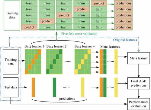
The stacking ensemble learning framework for estimating forest AGB is shown in Figure 1. In the two-layer stacking structure, the first layer included n base learners, and the second layer used a linear or nonlinear algorithm called a meta learner to combine the predictions of base learners. All data were randomly split into training data (80%) and test data (20%). The training data were further divided into five folds. In each of the five iterations, four folds were chosen for training base learners, whereas the remaining folds were held out for AGB prediction. The five-fold cross-validated predictions were called meta-features and served as input variables of the meta learner. When original features were not included in the stacking, the number of variables for training the meta learner equaled the number of base learners. The base learners were then refitted using all training data, and the refitted models were applied to the test data to generate meta-features or inputs of the meta learner. Final AGB predictions were obtained by a meta learner, and their accuracies were evaluated based on test data. To reduce the impacts of random splitting on the evaluation results, the above procedures were repeated 50 times.

Figure 1. Framework of stacking ensemble procedures for estimating forest AGB.

In this study, in addition to the evaluation of stacking using all data, we examined the performance of stacking models in estimating forest AGB for four forest types that had more than 1000 AGB samples, including EBF, DBF, WSA and SAV.

2.3.1. Base learners

The multivariate adaptive regression splines (MARS), support vector regression (SVR), multilayer perceptron (MLP) model, RF, extremely randomized trees (ERT) model, GBRT, SGB, and CatBoost regression algorithms were used as candidate base learners.

Since the combinations of base learners with high accuracy and diversity could maximize the generalization accuracy (Zhou 2009; Bin et al. 2020; Fan, Xiao, and Wang 2014), we selected CatBoost as one base learner due to its demonstrated better performance than the other candidate base learners (Zhang et al. 2020). The diversity among base learners was measured using Spearman’s rank correlation coefficient. Prediction errors of base learners had a lower correlation or even they were uncorrelated, suggesting that these learners skilled differently and thus corresponded to a higher diversity (Ma and Dai 2016). Afterward, we calculated the average of Spearman’s rank correlations among eight candidate base learners for 50 runs based on the prediction results from Zhang et al. (2020) and then selected the base learner with the lowest correlation with the CatBoost model as the second base learner. Similarly, the third base learner had the lowest mean correlation with the first two base learners. Through repeating the process, the remaining base learners were gradually added into the stacking model.

In addition, some studies have suggested that a few base learners instead of all available learners should be stacked together, and 3 or 4 base learners might be optimal (Zhou, Wu, and Tang 2002; Breiman 1996; Cho et al. 2020). Therefore, we attempted to stack 3–5 base learners and examined their performance for AGB estimation. The order of base learners selected under each forest type scenario is shown in Table 1. The stacking model with 3 base learners indicates that the first 3 learners were combined, and similarly, stacking with 5 base learners indicates that the first 5 base learners were used. Under all these scenarios, at least one homogeneous ensemble algorithm was selected as the base learners. To fully explore the stacking performance, we also used three individual learners, MARS, MLP, and SVR, as base learners, similar to many ensemble algorithms, and assessed the performance of associated stacking models in estimating forest AGB.

Table 1. Selected base learners, meta learner, and original features for stacking under five scenarios

Forest type	Base learners (from 1^st – 5^th)	Selected original features	Meta learner
All	CatBoost, MARS, MLP, GBRT, SVR	TC-Mean, CH, Temp, Prec, TC-Std, NPP	Ridge, RF
EBF	CatBoost, MLP, MARS, GBRT, SVR	TC-Mean, Prec, DEM, Temp, NPP, CH	Ridge, RF
DBF	CatBoost, MARS, GBRT, MLP, SVR	TC-Mean, Prec, Temp, DEM, NPP, TempChg	Ridge, RF
WSA	CatBoost, MARS, SVR, GBRT, MLP	TC-Mean, Prec, Temp, DEM, NPP, TempChg	Ridge, RF
SAV	CatBoost, MARS, MLP, GBRT, SVR	TC-Mean, Prec, NPP, DEM, Temp, TempChg	Ridge, RF

EBF, evergreen broadleaf forest; DBF, deciduous broadleaf forest; WSA, woody savanna; and SAV, savanna.

2.3.2. Meta learners

Simple linear models such as ridge and lasso regression are often used as the meta model, and they can provide a smooth interpretation of the predictions of base models (Cho et al. 2020). In this study, we also included ridge and lasso as meta learners in stacking. Additionally, original features that might improve the prediction results were incorporated as well (Pernía-Espinoza et al. 2018). RF and MLP could capture the nonlinear relationships between original features and forest biomass and were thus employed as meta learners in this study (Healey et al. 2018). We ranked the original features or variables used to train the base learners by feature importance values provided by the CatBoost, ERT, GBRT, SGB, MARS and RF algorithms (Zhang et al. 2020) and used six important features as additional inputs of the meta learner in stacking models. The selected original features under different scenarios are shown in Table 1.

Moreover, we initially tested the performance of ridge, lasso, MLP and RF algorithms as meta learners and found that lasso and MLP provided better prediction results than ridge and RF (Nath and Sahu 2019). Therefore, the ridge and RF were chosen as meta learners of stacking, and their performance in estimating AGB, when combined with different base learners, was explored (Table 1).

2.4. Forest AGB mapping

To further explore the performance of stacking models in AGB estimation, we generated the global forest AGB maps based on the optimal stacking model (Stacking AGB) and optimal base learner (CatBoost AGB), respectively, and then compared the spatial distribution of Stacking AGB with two other AGB maps including CatBoost AGB and global AGB map generated by fusion of multiple biomass maps (Fusion AGB) (Zhang and Liang 2020).

2.5. Accuracy assessment

Common metrics, including R² value, root mean square error (RMSE), and bias, were used to evaluate the accuracy of AGB predictions. They were calculated as:

(1) $R^2\left(y,\hat{y}\right)=1-\frac{{\sum }_{i=1}^N{\left(y_i-{\hat{y}}_i\right)}^2}{{\sum }_{i=1}^N{\left(y_i-\bar{y}\right)}^2}$(1)

(2) $RMSE\left(y,\hat{y}\right)=\sqrt{\frac{{\sum }_{i=1}^N{\left(y_i-{\hat{y}}_i\right)}^2}{N}}$(2)

(3) $bias\left(y,\hat{y}\right)=\frac{{\sum }_{i=1}^N\left(y_i-{\hat{y}}_i\right)}{N}$(3)

where $y$ represents the reference AGB,$\bar{y}$ denotes the mean value of the reference AGB, $\hat{y}$ is the predicted AGB using the models, and N is the number of samples. The model with higher $R^2$ value and lower RMSE and bias is preferred for AGB estimation.

In addition, the relative improvement (RI) in stacking performance for AGB estimation compared with the optimal base learner was quantified (Sun and Li 2020).

(4) $I_{R^2}=\frac{R_s^2-R_b^2}{R_b^2}\ast 100\mathrm{\%}$(4)

(5) $I_{RMSE}=\frac{RMS{E}_b-RMS{E}_s}{RMS{E}_b}\ast 100\mathrm{\%}$(5)

(6) $I_{bias}=\frac{\left|bia{s}_b\right|-\left|bia{s}_s\right|}{\left|bia{s}_b\right|}\ast 100\mathrm{\%}$(6)

where $I_{R^2}$, $I_{RMSE}$, and represent the RI in R², RMSE, and bias, respectively. The subscript s represents the stacking model, and b indicates the base learner.

3. Results

3.1. Performance of stacking models for forest AGB estimation

The average R², RMSE, and bias values of the five base learners and different stacking models obtained over 50 runs using all data are shown in Table 2. The CatBoost model outweighed the other base learners for AGB prediction and achieved an accuracy with an R² value of 0.70, RMSE of 47.19 Mg/ha and bias of 0.12 Mg/ha, which was the benchmark for evaluating the relative performance of stacking models in which CatBoost was contained. Similarly, MLP had an overall better performance than MARS and SVR and was therefore used to evaluate the RI of stacking in which the first layers were MARS, MLP, and SVR.

Table 2. Model assessments in R², RMSE and bias

Model	Meta-features			Meta- and original features			Relative improvement (%)
	R^2	RMSE(Mg/ha)	Bias(Mg/ha)	R^2	RMSE(Mg/ha)	Bias(Mg/ha)	R^2	RMSE	Bias
CatBoost	0.70	47.19	0.12	−	−	−	−	−	−
GBRT	0.69	48.01	0.07	−	−	−	−	−	−
MLP	0.62	53.43	−0.56	−	−	−	−	−	−
MARS	0.53	59.39	0.27	−	−	−	−	−	−
SVR	0.59	55.17	3.09	−	−	−	−	−	−
CatBoost + MARS + MLP (Ridge)	0.70	47.22	0.06	0.70	47.21	0.06	−0.05	−0.05	49.80
CatBoost + MARS + MLP (RF)	0.68	48.84	0.09	0.70	47.07	0.08	0.22	0.26	35.17
MARS + MLP + SVR (Ridge)	0.64	51.90	0.05	0.64	51.87	0.04	3.54	2.87	91.50
MARS + MLP + SVR (RF)	0.61	53.57	−0.02	0.67	49.44	0.04	8.96	7.46	92.70
CatBoost + MARS + MLP + GBRT (Ridge)	0.70	46.95	0.09	0.70	46.95	0.09	0.42	0.50	22.95
CatBoost + MARS + MLP + GBRT (RF)	0.69	47.93	0.11	0.70	46.82	0.13	0.66	0.78	−6.48
CatBoost + MARS + MLP + GBRT + SVR (Ridge)	0.70	46.96	0.09	0.70	46.96	0.09	0.40	0.48	22.12
CatBoost + MARS + MLP + GBRT+ SVR (RF)	0.69	47.66	0.10	0.70	46.85	0.13	0.62	0.72	−10.46

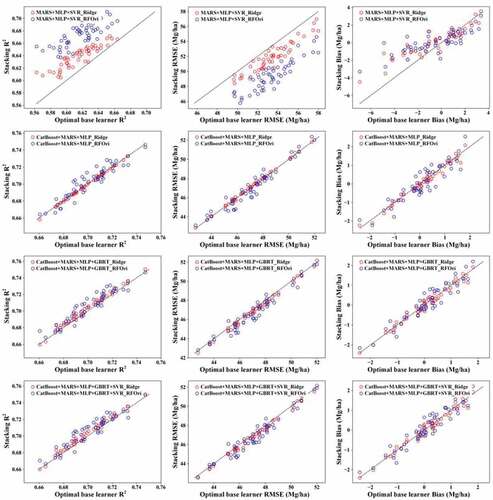
Consistent with some previous studies, the results of this study indicated that the incorporation of original features in stacking slightly improved the estimates (Pernía-Espinoza et al. 2018), mainly by decreasing RMSE. Moreover, stacking using the RF model and original features (RFOri) provided a more accurate estimation than stacking with ridge and original features (Table 2). In contrast, the stacking using ridge as a meta learner provided more accurate results than stacking using the RF model when original features were not considered inputs of the meta learner. Therefore, the RI shown in Table 2 for ridge-related stacking models was based on the ridge learner without original features, and the RI for RF-related models was based on RFOri.

RFOri produced the most accurate estimates of forest AGB for all combinations of base learners, whereas the performance of the ridge model, ridge model with original features, and RF model without original features was slightly worse in terms of R² and RMSE (Table 2 and Figure 2). Furthermore, the stacking using RFOri obtained a more accurate estimation of forest AGB than the optimal base learner, suggesting that stacking could improve the AGB estimation from multiple remote sensing datasets. For the base learner combination, MLP, MARS, and SVR, stacking using RFOri improved the estimation by 8.96%, 7.46% and 92.70% in terms of R², RMSE, and bias, respectively. However, when four or five base learners were used, we found that stacking using RFOri produced larger bias than the other stacking models (Table 2).

Figure 2. Comparing the performance of stacking using ridge (Ridge) and stacking using RF, as well as original features (RFOri) with those obtained by the optimal base learner.

With meta-features alone, stacking models using the ridge model as the meta learner provided better results than those based on RF, as well as the optimal base learner, despite being less accurate than stacking models using RFOri (Figure 2). The maximum RI was 3.54% for R² and 2.87% for RMSE, achieved by stacking using MARS, MLP, and SVR as base learners. For bias, the average RI was more than 22.12%, which suggested that stacking could improve the estimates, particularly by reducing the bias. Using CatBoost, MARS, and MLP as base learners, stacking obtained similar results to the CatBoost model in terms of R² and RMSE but decreased the bias by 49.8% (Table 2).

Either using ridge or RFOri as the meta model, the stacking of MARS, MLP, and SVR significantly improved the results relative to the best base learner (Figure 2). This was consistent with the viewpoint that base learners should be mediocre learners, with an average performance of approximately 0.5–0.6; therefore, ensemble learners were better than the best base learners (Lasisi and Attoh-Okine 2019). For the stacking models containing CatBoost, which was a strong base learner, the results were slightly better than the optimal base learner; however, they did not suggest that stacking models using strong base learners should not be used since they could significantly improve the bias of estimates (Table 2).

3.2. Performance of stacking for different forest types

For all forest types, including EBF, DBF, WSA, and SAV, CatBoost remained the optimal base learner, while the SVR predictions were generally better than the MARS and MLP for AGB predictions. Figure 3 shows the average R², RMSE and bias achieved by stacking using ridge as the meta learner for 50 runs, and Figure 4 shows the boxplot of R², RMSE and bias for 50 runs. The results suggested that stacking MARS, MLP, and SVR improved the AGB estimation with increases in R² and decreases in RMSE and bias. The average RI in R² was 4.68% for EBF, 4.56% for DBF, 4.07% for WSA, and 4.68% for SAV (Figure 3 and Figure 4). In contrast, the stacking model in which CatBoost was one of the base learners obtained similar results to the optimal base learner CatBoost, indicating that stacking did not significantly improve the results in terms of R² and RMSE. However, all stacking models provided less biased AGB prediction than CatBoost and SVR, which confirmed that stacking improved the estimation by reducing the bias.

Figure 3. Performance of stacking in estimating AGB in terms of R², RMSE, and bias for EBF, DBF, WSA, and SAV.

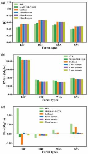
Figure 4. Boxplots depicting the relative improvement in R², RMSE, and bias achieved by stacking for AGB estimation in EBF, DBF, WSA, and SAV.

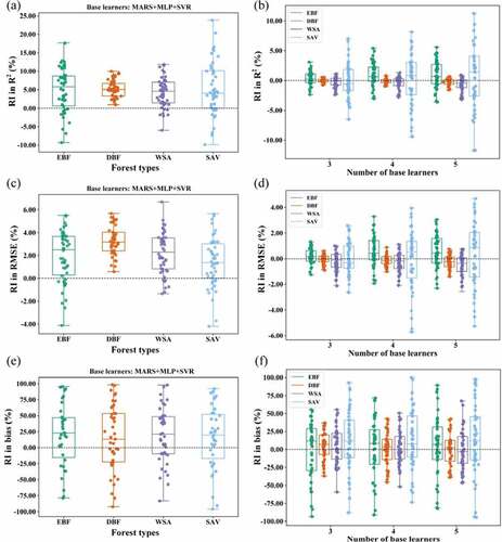
For EBF, all stacking models improved the performance in terms of the R², RMSE, and bias values compared with the optimal base learner, and the improvement was slightly different with the number of base learners used. When 3 base learners were included in stacking, the RI in R², RMSE, and bias were 0.22%, 0.13%, and 89.93%, respectively. Stacking using 5 base learners had RIs in R², RMSE, and bias of 1.00%, 0.59%, and 87.36%, respectively. The combination of four base learners, including CatBoost, MARS, MLP, and GBRT, had the best performance in terms of R² and RMSE (Figure 4). For DBF and WSA, CatBoost performed better than EBF, with a relatively larger R² and lower RMSE and a particularly lower bias. Under this condition, the stacking of CatBoost and other base learners did not lead to improved results except that stacking provided lower biased results in WSA (Figure 3 and Figure 4). The estimated results tended to become worse as the number of base learners used in stacking increased (Figure 4). These results indicated that when bias achieved by an algorithm was low, stacking of several learning algorithms might not be useful for further improving the accuracy of AGB estimation. For SAV, all base learners were weak learners with an R² of less than 0.48, and stacking indeed improved the results. With more base learners, the improvement of the stacking model in estimating forest AGB was greater. The bias decreased from 0.73 achieved by CatBoost to 0.06 achieved by stacking with five base learners, with an RI of 91.89%.

Despite the large differences in the performance of stacking models for different forest types, the combination of MARS, MLP, and SVR using stacking greatly improved the results compared with the optimal base learner SVR.

3.3. Global forest AGB maps generated using stacking

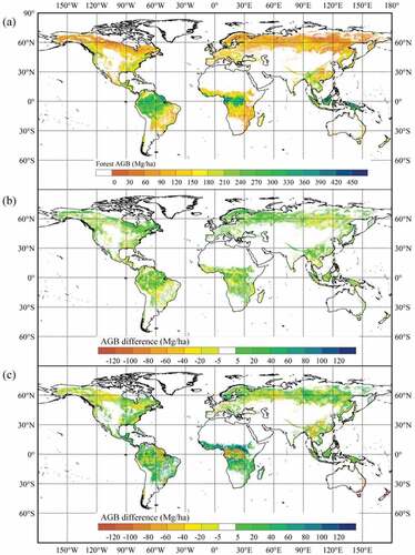
Based on the optimal stacking model (CatBoost + MARS + MLP + GBRT (Ridge) in Table 2) and base learner CatBoost, global AGB maps were generated for the 2000s from multiple remotely sensed data (Figure 5). The Stacking AGB map showed that tropical and subtropical forests stocked the most carbon in AGB per hectare, whereas the carbon stocks were lower in boreal and temperate forests. Compared with CatBoost AGB, Stacking AGB was higher in most regions with high biomass values and almost lower in regions with low biomass values, which suggested that stacking provided more reasonable AGB maps than optimal base learner. However, the difference in the spatial distribution of Stacking AGB and Fusion AGB was evident. Fusion AGB provided higher AGB in Oceania and Africa.

Figure 5. Spatial distributions of Stacking AGB for the 2000s (a), and difference maps obtained by subtracting the CatBoost AGB (b) and Fusion AGB (c) from Stacking AGB. Masked pixels denote areas with less than 10% forest cover.

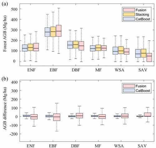
Figure 6 showed the estimated Stacking AGB, CatBoost AGB, and Fusion AGB values for different forest types. The results suggested that the three AGB maps, particularly Stacking AGB and CatBoost AGB, had similar statistical distributions for all forest types. Estimated AGB values in EBF were larger than those in ENF, DBF, MF, WSA, and SAV. Compared with the AGB difference obtained by subtracting the CatBoost AGB from Stacking AGB, AGB differences between Stacking AGB and Fusion AGB were larger (Figure 6). However, the median values of AGB difference between CatBoost and Stacking AGB were 5.86 Mg/ha for ENF, 3.99 Mg/ha for EBF, 1.62 Mg/ha for DBF, 4.68 Mg/ha for MF, 1.92 Mg/ha for WSA, and 0 Mg/ha for SAV. The median values of AGB difference between Fusion and Stacking AGB were −3.82 Mg/ha, −5.13 Mg/ha, 7.20 Mg/ha, −0.78 Mg/ha, 3.28 Mg/ha, and 2.80 Mg/ha for ENF, EBF, DBF, MF, WSA, and SAV, respectively.

Figure 6. Boxplot showing the AGB estimated by CatBoost, Stacking and Fusion (a) and AGB difference obtained by subtracting the CatBoost AGB and Fusion AGB from Stacking AGB (b) for different forest types.

4. Discussion

In recent decades, many studies have exploited complementary information from multiple remotely sensed data to improve AGB estimation. However, the effect of taking the advantage of diverse algorithms on the accurate estimation of forest AGB remains underexplored. In this study, we integrated several machine learning algorithms using stacking to estimate AGB from multiple satellite-derived data products. The results of this study showed that stacking models could generally improve the accuracy of AGB predictions, by greatly reducing the bias of estimates and slightly improving the R² and RMSE values. Therefore, if the main objective is to reduce the bias of estimates, such as for the retrieval of land surface parameters from satellite-derived data, stacking provides an effective way to achieve the goal. However, when the bias achieved by an optimal algorithm is low (e.g. DBF), the prediction accuracy cannot be further improved by stacking. In this situation, the base model rather than the stacking model should be used given its lower complexity (e.g. simple to train and interpret). Homogeneous ensemble methods such as RF and gradient boosting tree-base algorithms that have higher prediction performances may be considered (Güneralp, Filippi, and Randall 2014; Mutanga, Adam, and Cho 2012; Zhao et al. 2019).

The base learner combination, MARS, MLP, and SVR, obtained much better improvement compared with the results obtained by stacking using CatBoost as one of the base learners, suggesting the necessity to consider ensemble algorithms for improvement of prediction accuracy. However, it should be noted that the stacking of MARS, MLP, and SVR still provided less accurate results than the homogeneous CatBoost model. This was partly because stacking was a way to fuse information or add information to estimation, not an intrinsically motivated algorithm. More advanced algorithms, such as deep learning, remains worth investigating in future studies (Reichstein et al. 2019).

Previous studies have suggested that the appropriate selection of base learners is important for stacking models. In this study, we used the correlation of prediction error to quantify diversity and to further select base learners. Some metrics, such as covariance, dissimilarity measure, chi-square measure and mutual information, could be used to measure the diversity of base learners in stacking in future studies (Dutta 2009). Some studies have selected base learners based on their differences in algorithm principles (Wang, Lu, and Feng 2020). However, this should not greatly affect the results, since several combination strategies used in this study were consistent with the selection in principle (e.g. MARS + MLP + SVR, CatBoost + MARS + MLP, and CatBoost + MARS + SVR in Table 2). To fully explore the feasibility of stacking for global forest AGB mapping, we generated AGB maps using the optimal stacking model on a global scale. Comparison results showed that stacking AGB was generally close to CatBoost AGB, with an AGB difference of less than 20 Mg/ha in most forest regions. Due to the urgent need to improve forest AGB estimation on regional and global scales, many studies have integrated multisource remotely sensed data by using various machine learning algorithms. Two typical examples were forest AGB maps covering tropical regions produced by Saatchi et al. (2011) based on the MaxEnt algorithm and by Baccini et al. (2012) based on the RF algorithm, which were also used by Liu et al. (2015) to generate global forest AGB maps by establishing the relationships between AGB and vegetation optical depth, and by Carvalhais et al. (2014) to calculate turnover times of carbon in terrestrial ecosystems. The existing AGB maps were almost produced by a specific algorithm rather than an ensemble of several algorithms. As suggested by Figure 5, the estimated AGB based only on CatBoost and that based on an ensemble of several algorithms under the stacking framework were different in both magnitude and spatial distribution, which indicated the uncertainties associated with the AGB modeling algorithms and the necessity to examine the uncertainties in future studies of AGB estimation or mapping. In our previous studies, systematic comparisons of existing regional and global forest AGB maps covering different continents (Zhang, Liang, and Yang 2019) and a detailed comparison of several global AGB maps (Zhang and Liang 2020) were performed. The results revealed large discrepancies in current AGB maps, which could be from field biomass, the choice and quality of remotely sensed data, and the highlighted uncertainties of AGB modeling algorithms.

5. Conclusion

In recent decades, many studies have estimated forest AGB by fusing multiple remotely sensed data using various algorithms. However, integrating several algorithms to improve AGB estimation has rarely been investigated. In this study, we examined the performance of the stacking ensemble algorithm, which can combine diverse learners, in estimating forest AGB from multiple remotely sensed datasets. Based on the diversity measured by Spearman’s rank correlation coefficient of prediction errors achieved by base learners, as well as accuracy, we selected five base learners and used a combination of 3–5 base learners with ridge and RF to estimate AGB. The evaluation results showed that the stacking model generally outweighed the optimal base model and improved the prediction results, particularly by decreasing the bias, and stacking using the RF model as the meta learner and important original features as inputs of the meta learner provided the most accurate estimation. However, it could lead to larger biased estimates with an increase in the number of base learners included in the stacking structure. In terms of R² and RMSE, only slight improvement of stacking in the prediction accuracy was found. The stacking of MARS, MLP, and SVR provided greatly improved results compared with the optimal base learner. The average RI in R² was 3.54% when we used all datasets without separating forest types, and the average RI in R² was 4.68% for EBF, 4.56% for DBF, 4.07% for WSA, and 4.68% for SAV. All stacking models had an RI bias of at least 22.12%, or even reaching more than 90% under some scenarios, except for DBF, where an optimal algorithm could provide low biased results. The results of this study demonstrated the capability of the stacking ensemble algorithm in reducing the bias in estimating AGB. In future studies, stacking could be utilized to retrieve AGB or other biophysical parameters from remotely sensed data if decreasing the bias was the main objective.

Data and codes availability statement

The data that supports the findings of this study is available at https://doi.org/10.5281/zenodo.5464675.

Disclosure statement

No potential conflict of interest was reported by the author(s).

Additional information

Funding

This work was supported in part by the National Natural Science Foundation of China (Grant No. 41801347) and the National Key Research and Development Program of China (2016YFA0600103 and 2018YFC1407103).

References

- Baccini, A., S. J. Goetz, W. S. Walker, N. T. Laporte, M. Sun, D. Sulla-Menashe, J. Hackler, et al. 2012. “Estimated Carbon Dioxide Emissions from Tropical Deforestation Improved by Carbon-density Maps.” Nature Climate Change 2 (3): 182–185. doi:10.1038/nclimate1354.
- Belgiu, M., and L. Drăguţ. 2016. “Random Forest in Remote Sensing: A Review of Applications and Future Directions.” ISPRS Journal of Photogrammetry and Remote Sensing 114 (Supplement C): 24–31. doi:10.1016/j.isprsjprs.2016.01.011.
- Bin, Y., W. Zhang, W. Tang, R. Dai, M. Li, Q. Zhu, and J. Xia. 2020. “Prediction of Neuropeptides from Sequence Information Using Ensemble Classifier and Hybrid Features.” Journal of Proteome Research 19 (9): 3732–3740. doi:10.1021/acs.jproteome.0c00276.
- Bouvet, A., S. Mermoz, T. Le Toan, L. Villard, R. Mathieu, L. Naidoo, and G. P. Asner. 2018. “An Above-ground Biomass Map of African Savannahs and Woodlands at 25m Resolution Derived from ALOS PALSAR.” Remote Sensing of Environment 206: 156–173. doi:10.1016/j.rse.2017.12.030.
- Breiman, L. 1996. “Stacked Regressions.” Machine Learning 24 (1): 49–64. doi:10.1007/BF00117832.
- Breiman, L. 2001. “Random Forests.” Machine Learning 45 (1): 5–32. doi:10.1023/a:1010933404324.
- Bühlmann, P., and T. Hothorn. 2007. “Boosting Algorithms: Regularization, Prediction and Model Fitting.” Statistical Science 22 (4): 477–505.
- Carreiras, J. M. B., S. Quegan, T. Le Toan, D. H. T. Minh, S. S. Saatchi, N. Carvalhais, M. Reichstein, and K. Scipal. 2017. “Coverage of High BIOMASS Forests by the ESA BIOMASS Mission under Defense Restrictions.” Remote Sensing of Environment 196: 154–162. doi:10.1016/j.rse.2017.05.003.
- Carvalhais, N., M. Forkel, M. Khomik, J. Bellarby, M. Jung, M. Migliavacca, M. Mu, et al. 2014. “Global Covariation of Carbon Turnover Times with Climate in Terrestrial Ecosystems.” Nature 514 (7521): 213–217. doi:10.1038/nature13731.
- Chave, J., S. J. Davies, O. L. Phillips, S. L. Lewis, P. Sist, D. Schepaschenko, J. Armston, et al. 2019. “Ground Data are Essential for Biomass Remote Sensing Missions.” Surveys in Geophysics 40 (4): 863–880. doi:10.1007/s10712-019-09528-w.
- Cho, D., C. Yoo, J. Im, Y. Lee, and J. Lee. 2020. “Improvement of Spatial Interpolation Accuracy of Daily Maximum Air Temperature in Urban Areas Using a Stacking Ensemble Technique.” Giscience & Remote Sensing 57 (5): 633–649. doi:10.1080/15481603.2020.1766768.
- Danielson, J. J., and D. B. Gesch. 2011. “Global Multi-resolution Terrain Elevation Data 2010 (GMTED2010).” In Open-File Report.
- de Almeida, C. T., L. S. Galvao, L. Aragao, A. D. J. Jphb Ometto, F. R. D. Pereira, L. Y. Sato, Lopes AP, de Alencastro Graça PM, de Jesus Silva CV, Ferreira-Ferreira J, Longo M, et al. 2019. “Combining LiDAR and Hyperspectral Data for Aboveground Biomass Modeling in the Brazilian Amazon Using Different Regression Algorithms.” Remote Sensing of Environment 232: 111323. doi:10.1016/j.rse.2019.111323.
- Divina, F., A. Gilson, F. Goméz-Vela, M. García Torres, and J. F. Torres. 2018. “Stacking Ensemble Learning for Short-term Electricity Consumption Forecasting.” Energies 11 (4): 949. doi:10.3390/en11040949.
- Dutta, H. 2009. Measuring Diversity in Regression Ensembles. Paper presented at the Proceedings of the 4th Indian International Conference on Artificial Intelligence, IICAI 2009, Tumkur, Karnataka, India, 16-18 December 2009.
- Fan, C., F. Xiao, and S. Wang. 2014. “Development of Prediction Models for Next-day Building Energy Consumption and Peak Power Demand Using Data Mining Techniques.” Applied Energy 127: 1–10. doi:10.1016/j.apenergy.2014.04.016.
- Fick, S. E., and R. J. Hijmans. 2017. “WorldClim 2: New 1-km Spatial Resolution Climate Surfaces for Global Land Areas.” International Journal of Climatology 37 (12): 4302–4315. doi:10.1002/joc.5086.
- Friedman, J. H. 2001. “Greedy Function Approximation: A Gradient Boosting Machine.” The Annals of Statistics 29 (5): 1189–1232. doi:10.1214/aos/1013203451.
- Friedman, J. H. 2002. “Stochastic Gradient Boosting.” Computational Statistics & Data Analysis 38 (4): 367–378. doi:10.1016/S0167-9473(01)00065-2.
- Gleason, C. J., and J. Im. 2012. “Forest Biomass Estimation from Airborne LiDAR Data Using Machine Learning Approaches.” Remote Sensing of Environment 125: 80–91. doi:10.1016/j.rse.2012.07.006.
- Güneralp, İ., A. M. Filippi, and J. Randall. 2014. “Estimation of Floodplain Aboveground Biomass Using Multispectral Remote Sensing and Nonparametric Modeling.” International Journal of Applied Earth Observation and Geoinformation 33: 119–126. doi:10.1016/j.jag.2014.05.004.
- Hansen, M. C., P. V. Potapov, R. Moore, M. Hancher, S. A. Turubanova, A. Tyukavina, D. Thau, et al. 2013. “High-resolution Global Maps of 21st-Century Forest Cover Change.” Science 342 (6160): 850–853. doi:10.1126/science.1244693.
- Harris, I., P. D. Jones, T. J. Osborn, and D. H. Lister. 2014. “Updated High-resolution Grids of Monthly Climatic Observations – The CRU TS3.10 Dataset.” International Journal of Climatology 34 (3): 623–642. doi:10.1002/joc.3711.
- Healey, S. P., W. B. Cohen, Z. Yang, Brewer, C. Kenneth, E. B. Brooks, N. Gorelick, A. J. Hernandez, Huang C., Hughes M. Joseph, Kennedy R. E., Loveland T. R., et al. 2018. “Mapping Forest Change Using Stacked Generalization: An Ensemble Approach”. Remote Sensing of Environment 204: 717–728. doi:10.1016/j.rse.2017.09.029.
- Houghton, R. A., F. Hall, and S. J. Goetz. 2009. “Importance of Biomass in the Global Carbon Cycle.” Journal of Geophysical Research: Biogeosciences 114 (G2): G00E3. doi:10.1029/2009JG000935.
- Huang, G., L. Wu, X. Ma, W. Zhang, J. Fan, X. Yu, W. Zeng, and H. Zhou. 2019. “Evaluation of CatBoost Method for Prediction of Reference Evapotranspiration in Humid Regions.” Journal of Hydrology 574: 1029–1041. doi:10.1016/j.jhydrol.2019.04.085.
- Kattenborn, T., J. Maack, F. Faßnacht, F. Enßle, J. Ermert, and B. Koch. 2015. “Mapping Forest Biomass from Space – Fusion of Hyperspectral EO1-hyperion Data and Tandem-X and WorldView-2 Canopy Height Models.” International Journal of Applied Earth Observation and Geoinformation 35: 359–367. doi:10.1016/j.jag.2014.10.008.
- Keeling, H. C., and O. L. Phillips. 2007. “The Global Relationship between Forest Productivity and Biomass.” Global Ecology and Biogeography 16 (5): 618–631. doi:10.1111/j.1466-8238.2007.00314.x.
- Lasisi, A., and N. Attoh-Okine. 2019. “Machine Learning Ensembles and Rail Defects Prediction: Multilayer Stacking Methodology.” ASCE-ASME Journal of Risk and Uncertainty in Engineering Systems, Part A: Civil Engineering 5 (4): 04019016. doi:10.1061/AJRUA6.0001024.
- Li, X., H. Lu, L. Yu, and K. Yang. 2018. “Comparison of the Spatial Characteristics of Four Remotely Sensed Leaf Area Index Products over China: Direct Validation and Relative Uncertainties.” Remote Sensing 10 (1): 148. doi:10.3390/rs10010148.
- Li, Y., M. Li, C. Li, and Z. Liu. 2020. “Forest Aboveground Biomass Estimation Using Landsat 8 and Sentinel-1A Data with Machine Learning Algorithms.” Scientific Reports 10 (1): 9952. doi:10.1038/s41598-020-67024-3.
- Liang, S. L., J. Cheng, K. Jia, B. Jiang, Q. Liu, Z. Q. Xiao, Y. J. Yao, et al. 2021. “The Global Land Surface Satellite (GLASS) Product Suite.” Bulletin of the American Meteorological Society 102 (2): E323–E37. doi:10.1175/BAMS-D-18-0341.1.
- Liang, S., X. Zhao, S. Liu, W. Yuan, X. Cheng, Z. Xiao, X. Zhang, et al. 2013. “A Long-term Global LAnd Surface Satellite (GLASS) Data-set for Environmental Studies.” International Journal of Digital Earth 6 (sup1): 5–33. doi:10.1080/17538947.2013.805262.
- Liu, Y., A. I. J. M. van Dijk, R. A. M. de Jeu, J. G. Canadell, M. F. McCabe, J. P. Evans, and G. Wang. 2015. “Recent Reversal in Loss of Global Terrestrial Biomass.” Nature Climate Change 5 (5): 470–474. doi:10.1038/nclimate2581.
- López-Serrano, P. M., C. A. López-Sánchez, -G. Á.-G. Juan, and J. García-Gutiérrez. 2016. “A Comparison of Machine Learning Techniques Applied to Landsat-5 TM Spectral Data for Biomass Estimation.” Canadian Journal of Remote Sensing 42 (6): 690–705. doi:10.1080/07038992.2016.1217485.
- Lu, D., Q. Chen, G. Wang, L. Liu, G. Li, and E. Moran. 2016. “A Survey of Remote Sensing-based Aboveground Biomass Estimation Methods in Forest Ecosystems.” International Journal of Digital Earth 9 (1): 63–105. doi:10.1080/17538947.2014.990526.
- Luo, S., C. Wang, X. Xi, S. Nie, X. Fan, H. Chen, X. Yang, D. Peng, Y. Lin, and G. Zhou. 2019. “Combining Hyperspectral Imagery and LiDAR Pseudo-waveform for Predicting Crop LAI, Canopy Height and Above-ground Biomass.” Ecological Indicators 102: 801–812. doi:10.1016/j.ecolind.2019.03.011.
- Ma, Z., and Q. Dai. 2016. “Selected an Stacking ELMs for Time Series Prediction.” Neural Processing Letters 44 (3): 831–856. doi:10.1007/s11063-016-9499-9.
- Mendes-Moreira, J., C. Soares, A. M. Jorge, and J. F. De Sousa. 2012. “Ensemble Approaches for Regression: A Survey.” ACM Computing Surveys 45 (1): 10. doi:10.1145/2379776.2379786.
- Mitchard, E. T., S. S. Saatchi, A. Baccini, G. P. Asner, S. J. Goetz, N. L. Harris, and S. Brown. 2013. “Uncertainty in the Spatial Distribution of Tropical Forest Biomass: A Comparison of Pan-tropical Maps.” Carbon Balance and Management 8 (1): 10. doi:10.1186/1750-0680-8-10.
- Mutanga, O., E. Adam, and M. A. Cho. 2012. “High Density Biomass Estimation for Wetland Vegetation Using WorldView-2 Imagery and Random Forest Regression Algorithm.” International Journal of Applied Earth Observation and Geoinformation 18: 399–406. doi:10.1016/j.jag.2012.03.012.
- Naimi, A. I., and L. B. Balzer. 2018. “Stacked Generalization: An Introduction to Super Learning.” European Journal of Epidemiology 33 (5): 459–464. doi:10.1007/s10654-018-0390-z.
- Nath, A., and G. K. Sahu. 2019. “Exploiting Ensemble Learning to Improve Prediction of Phospholipidosis Inducing Potential.” Journal of Theoretical Biology 479: 37–47. doi:10.1016/j.jtbi.2019.07.009.
- Neumann, M., S. S. Saatchi, L. M. H. Ulander, and J. E. S. Fransson. 2012. “Assessing Performance of L- and P-Band Polarimetric Interferometric SAR Data in Estimating Boreal Forest Above-ground Biomass.” IEEE Transactions on Geoscience and Remote Sensing 50 (3): 714–726. doi:10.1109/TGRS.2011.2176133.
- Pernía-Espinoza, A., J. Fernandez-Ceniceros, J. Antonanzas, R. Urraca, and F. J. Martinez-de-pison. 2018. “Stacking Ensemble with Parsimonious Base Models to Improve Generalization Capability in the Characterization of Steel Bolted Components.” Applied Soft Computing 70: 737–750. doi:10.1016/j.asoc.2018.06.005.
- Qi, W., S. Saarela, J. Armston, G. Ståhl, and R. Dubayah. 2019. “Forest Biomass Estimation over Three Distinct Forest Types Using TanDEM-X InSAR Data and Simulated GEDI Lidar Data.” Remote Sensing of Environment 232: 111283. doi:10.1016/j.rse.2019.111283.
- Reichstein, M., G. Camps-Valls, B. Stevens, M. Jung, J. Denzler, and N. Carvalhais, Prabhat. 2019. “Deep Learning and Process Understanding for Data-driven Earth System Science.” Nature 566 (7743): 195–204. doi:10.1038/s41586-019-0912-1.
- Réjou-Méchain, M., H. C. Muller-Landau, M. Detto, S. C. Thomas, T. Le Toan, S. S. Saatchi, J. S. Barreto-Silva, et al. 2014. “Local Spatial Structure of Forest Biomass and Its Consequences for Remote Sensing of Carbon Stocks.” Biogeosciences 11 (23): 6827–6840. doi:10.5194/bg-11-6827-2014.
- Running, S., and M. Zhao. 2019. “MOD17A3HGF MODIS/Terra Net Primary Production Gap-Filled Yearly L4 Global 500 M SIN Grid V006.“ In: NASA EOSDIS Land Processes DAAC. Accessed from 03 May 2020. https://doi.org/10.5067/MODIS/MOD17A3HGF.006
- Saatchi, S. S., N. L. Harris, S. Brown, M. Lefsky, E. T. A. Mitchard, W. Salas, B. R. Zutta, et al. 2011. “Benchmark Map of Forest Carbon Stocks in Tropical Regions across Three Continents.” Proceedings of the National Academy of Sciences, 108 (24): 9899–9904. doi:10.1073/pnas.1019576108.
- Schmitt, C. B., N. D. Burgess, L. Coad, A. Belokurov, C. Besançon, L. Boisrobert, A. Campbell, et al. 2009. “Global Analysis of the Protection Status of the World’s Forests.” Biological Conservation 142 (10): 2122–2130. doi:10.1016/j.biocon.2009.04.012.
- Simard, M., N. Pinto, J. B. Fisher, and A. Baccini. 2011. “Mapping Forest Canopy Height Globally with Spaceborne Lidar.” Journal of Geophysical Research: Biogeosciences 116 (G4): G04021. doi:10.1029/2011JG001708.
- Sulla-Menashe, D., J. M. Gray, S. Parker Abercrombie, and M. A. Friedl. 2019. “Hierarchical Mapping of Annual Global Land Cover 2001 to Present: The MODIS Collection 6 Land Cover Product.” Remote Sensing of Environment 222: 183–194. doi:10.1016/j.rse.2018.12.013.
- Sun, W., and Z. Li. 2020. “Hourly PM2.5 Concentration Forecasting Based on Mode Decomposition-recombination Technique and Ensemble Learning Approach in Severe Haze Episodes of China.” Journal of Cleaner Production 263: 121442. doi:10.1016/j.jclepro.2020.121442.
- Tyralis, H., G. Papacharalampous, A. Burnetas, and A. Langousis. 2019. “Hydrological Post-processing Using Stacked Generalization of Quantile Regression Algorithms: Large-scale Application over CONUS.” Journal of Hydrology 577: 123957. doi:10.1016/j.jhydrol.2019.123957.
- Wang, R., S. Lu, and W. Feng. 2020. “A Novel Improved Model for Building Energy Consumption Prediction Based on Model Integration.” Applied Energy 262: 114561. doi:10.1016/j.apenergy.2020.114561.
- Wang, Y., X. Wu, and X. Mo. 2013. “A Novel Adaptive-weighted-average Framework for Blood Glucose Prediction.” Diabetes Technology & Therapeutics 15 (10): 792–801. doi:10.1089/dia.2013.0104.
- Wolpert, D. H. 1992. “Stacked Generalization.” Neural Networks 5 (2): 241–259. doi:10.1016/s0893-6080(05)80023-1.
- Wulder, M. A., J. C. White, R. F. Nelson, E. Næsset, H. Ole Ørka, N. C. Coops, T. Hilker, C. W. Bater, and T. Gobakken. 2012. “Lidar Sampling for Large-area Forest Characterization: A Review.” Remote Sensing of Environment 121: 196–209. doi:10.1016/j.rse.2012.02.001.
- Xiao, Z., S. Liang, J. Wang, P. Chen, X. Yin, L. Zhang, and J. Song. 2014. “Use of General Regression Neural Networks for Generating the GLASS Leaf Area Index Product from Time-series MODIS Surface Reflectance.” IEEE Transactions on Geoscience and Remote Sensing 52 (1): 209–223. doi:10.1109/TGRS.2013.2237780.
- Xiao, Z., S. Liang, J. Wang, Y. Xiang, X. Zhao, and J. Song. 2016. “Long-time-series Global Land Surface Satellite Leaf Area Index Product Derived from MODIS and AVHRR Surface Reflectance.” IEEE Transactions on Geoscience and Remote Sensing 54 (9): 5301–5318. doi:10.1109/TGRS.2016.2560522.
- Yang, P., Y. H. Yang, B. B. Zhou, and A. Y. Zomaya. 2010. “A Review of Ensemble Methods in Bioinformatics.” Current Bioinformatics 5 (4): 296–308. doi:10.2174/157489310794072508.
- Zhai, B., and J. Chen. 2018. “Development of a Stacked Ensemble Model for Forecasting and Analyzing Daily Average PM2.5 Concentrations in Beijing, China.” Science of the Total Environment 635: 644–658. doi:10.1016/j.scitotenv.2018.04.040.
- Zhang, Y., J. Ma, S. Liang, X. Li, and M. Li. 2020. “An Evaluation of Eight Machine Learning Regression Algorithms for Forest Aboveground Biomass Estimation from Multiple Satellite Data Products.” Remote Sensing 12 (24): 4015. doi:10.3390/rs12244015.
- Zhang, Y., and S. Liang. 2020. “Fusion of Multiple Gridded Biomass Datasets for Generating a Global Forest Aboveground Biomass Map.” Remote Sensing 12 (16): 2559. doi:10.3390/rs12162559.
- Zhang, Y., S. Liang, and L. Yang. 2019. “A Review of Regional and Global Gridded Forest Biomass Datasets.” Remote Sensing 11 (23): 2744. doi:10.3390/rs11232744.
- Zhao, Q., S. Yu, F. Zhao, L. Tian, and Z. Zhao. 2019. “Comparison of Machine Learning Algorithms for Forest Parameter Estimations and Application for Forest Quality Assessments.” Forest Ecology and Management 434: 224–234. doi:10.1016/j.foreco.2018.12.019.
- Zhou, Z.-H., J. Wu, and W. Tang. 2002. “Ensembling Neural Networks: Many Could Be Better than All.” Artificial Intelligence 137 (1–2): 239–263. doi:10.1016/S0004-3702(02)00190-X.
- Zhou, Z.-H. 2009. “Ensemble Learning.” In Encyclopedia of Biometrics, edited by S. Z. Li, and A. Jain, 270–273. Boston, MA: Springer US.
- Zolkos, S. G., S. J. Goetz, and R. Dubayah. 2013. “A Meta-analysis of Terrestrial Aboveground Biomass Estimation Using Lidar Remote Sensing.” Remote Sensing of Environment 128: 289–298. doi:10.1016/j.rse.2012.10.017.