Surface deformation extraction from small baseline subset synthetic aperture radar interferometry (SBAS-InSAR) using coherence-optimized baseline combinations

ABSTRACT

Surface deformation data can be used to provide early warnings of geohazards and are useful in a variety of research fields. The Small BAseline Subset InSAR (SBAS-InSAR) boosts the data sampling rate and improves the accuracy of deformation extraction by restricting the temporal and spatial baselines. However, various factors, such as the types of ground objects and seasons, affect the coherence between SAR images. Traditional SBAS-InSAR employs a fixed temporal baseline, which does not guarantee good coherence and might lead to decorrelation. In this paper, we propose that instead of using a fixed temporal baseline, we directly use the average coherence between SAR images as the baseline constraint index to perform an optimized selection of SBAS-InSAR interferometric pairs, ensuring good coherence of the interferometric pairs and improving the quality of the interferometric fringes. The proposed approach was used to extract surface deformation in two test experiment areas: Houston and Sydney. Compared with the conventional SBAS-InSAR and GPS data, the standard deviation of error of Houston and Sydney dropped from 0.813 to 0.589 and 0.291 to 0.246, respectively; the root mean square error (RMSE) decreased from 1.082 to 1.041 and 0.485 to 0.334, respectively, indicating that the proposed method has better surface deformation extraction accuracy. After demonstrating the accuracy of the proposed method, it was applied to Pingxiang area, a mining city in China, to effectively extract and analyze the surface deformation induced by mining activities, which proves the universality of this method in different scenarios.

KEYWORDS:

• Temporal baseline
• SBAS-InSAR
• coherence
• ground deformation

1. Introduction

Surface deformation caused by human activities (i.e. mining, groundwater extraction, and constructions) and natural processes (i.e. earthquake and landslide) seriously threatens the safety of people and surface infrastructure; surface deformation data are useful in many research fields including geology (Bürgmann, Rosen, and Fielding 2000; Fujiwara et al. 1998), hydrology (Galloway and Burbey 2011), cryosphere (Muhammad and Tian 2020; Tian et al. 2017), etc. Therefore, it is imperative to effectively monitor ground deformation (Amelung et al. 1999; Dinar et al. 2021; Syvitski et al. 2009). Traditional methods such as leveling, GPS (Global Positioning System), and others exhibit certain limitations (Cigna and Tapete 2021; Hong et al. 2012). Synthetic aperture radar (SAR) interferometry (InSAR) employs the phase information of the SAR image to obtain surface elevation and deformation and has advantages of wide and fast coverage, as well as precise deformation recognition capability (Li, Zhou, and Ma 2000; Massonnet and Feigl 1998; Wang et al. 2020; Wright and Stow 1999). Conventional InSAR technology suffers from decorrelation and atmospheric phase delay, resulting in a limited accuracy (Liu 2003; Zebker, Rosen, and Hensley 1997). The small baseline subset InSAR (SBAS-InSAR) adopts small threshold constrained spatial-temporal baseline to increase the data sampling rate (Berardino et al. 2002), which considerably improves the monitoring accuracy, and has been widely used in large-scale surface deformation monitoring and related applications.

To retrieve the surface deformation using SBAS-InSAR, the small baseline subsets should first be selected using spatial and temporal baseline thresholds. At present, there are three primary selection methods: 1. Only setting temporal baseline threshold, such as Fariba’s inversion of surface stability in Yukon Territory, Canada (Mohammadimanesh et al. 2019). This method is commonly utilized in areas with low coherence, such as mountainous and densely forested regions, to effectively reduce temporal decorrelation. 2. Only setting spatial baseline threshold, as in Chaussard’s deformation inversion and attribution in western Indonesia (Chaussard et al. 2013) and Kim’s extraction of deformation patterns in Tuscon (Kim et al. 2015). This method effectively reduces the impact of terrain error, but it requires high coherence of data itself, which is better suited to long wavelength radar data. 3. Setting both temporal and spatial baseline thresholds, which is by far the most commonly used method and has a wide range of applications. It is adopted in Zhao’s description of landslide deformation time series (Zhao et al. 2012), the extraction of large-scale surface deformation by Tizzani et al. (2007), Chaussard et al. (2014), Bateson et al. (2015), and Zhao et al. (2016), and the extraction of urban deformation in Shanghai, Shenzhen, and Wuhan by Dong et al. (2014), Xu et al. (2016), and Zhou et al. (2017).

These applications usually set a short temporal baseline threshold to ensure coherence. It is an empirical approach based on the assumption that tiny changes in ground objects over a short time interval do not induce decorrelation. However, it cannot be guaranteed that all interferometric pairs have good coherence. For example, vegetation coverage is sparse in winter, and the coherence between images is good even with a longer time interval; when it comes to summer, with denser vegetation and precipitation, even adjacent acquisitions may exhibit poor coherence. The fixed temporal baseline threshold of conventional SBAS-InSAR cannot handle these scenarios adequately and may lead to decorrelation errors. Earlier reports such as Zhou et al. (2017) and Mohammadimanesh et al. (2019) also realized this issue; thus, although Zhou et al. (2017) set a fixed temporal baseline of 200 days, he manually removed interferometric pairs with low coherence; Mohammadimanesh et al. (2019) dynamically set its temporal baseline threshold at 72 days during the thawing season (July to October) and 24 days in the early spring and freezing season to maintain good coherence over permafrost areas. However, these operations added to the processing complexity. In light of the above-mentioned issue, this paper proposes to directly use the average coherence of interferometric pairs instead of the temporal baseline as the threshold index to optimize the baseline combination and then use the optimized combination for subsequent SBSA-InSAR processing to improve the accuracy of deformation extraction. Two experiments are designed, including the test experiment in Houston and Sydney and a case study in Pingxiang, China. In the test experiment, the deformation results of conventional SBAS-InSAR and GPS data are compared to demonstrate the superiority of this method. Then, the method is utilized in Pingxiang, a mining city, to efficiently extract and analyze the surface deformation, which proves the universality of the method in different scenarios.

2. Materials and methods

2.1. Data

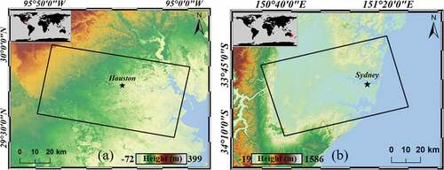
The study areas included Houston, United States, and Sydney, Australia, which belong to different hemispheres, as shown in Figure 1. The data used for both areas are all C-band interferometric wide swath (IW) mode Single Look Complex (SLC) SAR images with VV (Vertical-Vertical) polarization of Sentinel-1 satellite. The path direction of Houston is descending, while that of Sydney is ascending with incident angles of 35.38° and 36.91°, respectively. The ground resolution after multilooking with a ratio of 5 × 1 (range × azimuth) was 20 m. A total of 30 images from January to December 2020 with an acquisition interval of 12 days of each study area were collected. All images were clipped according to the scope of the study areas for further processing.

Figure 1. Diagram of study area: Houston (a) and Sydney (b), the black rectangle delineates the data coverage, and the background is SRTM DEM.

2.2. Principle and method

2.2.1. InSAR coherence and its impact on deformation measurement

The coherence in InSAR is defined as the cross-correlation coefficient in the registration of two complex images (Touzi et al. 1999). It is a versatile InSAR by-product with many uses (Chaabani et al. 2018; Chini et al. 2019; Van der Sanden, Short, and Drouin 2018; Wang et al. 2020); it is also an important index, which can be used to describe the quality of the interferometric phase. The higher the coherence, the more reliable the phase information. Better coherence can help to eliminate phase discontinuity that introduces errors in the subsequent filtering and unwrapping process, yielding more accurate deformation results.

The coherence of an image point $\left(i,j\right)$ can be expressed as

(1) ${\gamma }_{(i,j)}=\frac{|\sum _{i=1}^m\sum _{j=1}^{n}M(i,j)S^{\ast }(i,j)|}{\sqrt{\sum _{i=1}^m\sum _{j=1}^n|M(i,j){|}^2\sum _{i=1}^m\sum _{j=1}^n|S(i,j){|}^2}},$(1)

where $M$ and $S$ are SAR acquisitions, $\ast$ indicates the complex conjugate, and $m$ and $n$ are the local window size for coherence calculation, with $\left(i,j\right)$ being the pixel coordinates in the slant range.

Generally, coherence is affected by many factors and can be summarized as follows (Zebker and Villasenor 1992):

(2) $\gamma ={\gamma }_{process}\cdot {\gamma }_{doppler}\cdot {\gamma }_{thermal}\cdot {\gamma }_{vol}\cdot {\gamma }_{temporal}\cdot {\gamma }_{geom},$(2)

where ${\gamma }_{process}$ is the decorrelation incurred during data processing flows, i.e. image misregistration, ${\gamma }_{doppler}$ is the Doppler centroid decorrelation,${\gamma }_{thermal}$ is the thermal noise decorrelation, and ${\gamma }_{vol}$ is the volumetric scattering decorrelation; the above four factors affect the entire scene of data, and cannot be mitigated by temporal or spatial baseline manipulations (Malinverni et al. 2014). ${\gamma }_{temporal}$ is temporal decorrelation. For repeat-pass interferometry, variations in the positions of ground objects and soil humidity during acquisitions introduce random phase delay, also known as temporal decorrelation (Ahmed et al. 2011; Ma et al. 2018). ${\gamma }_{geom}$ is geometric decorrelation. Longer spatial baseline between acquisitions causes larger variation in the looking angle of the sensor, which may lead to geometric decorrelation (Gatelli et al. 1994).

2.2.2. Coherence distribution between SAR images

SBAS-InSAR alleviates ${\gamma }_{temporal}$ and ${\gamma }_{geom}$ by thresholding temporal and spatial baselines, reducing the influence of decorrelation, and improving the accuracy of surface deformation inversion. According to the principle of InSAR, an interferometric pair requires the participation of two separate SAR acquisitions. A total of $N$ SAR images can generate $\frac{N\ast \left(N-1\right)}{2}$ interferometric pairs. 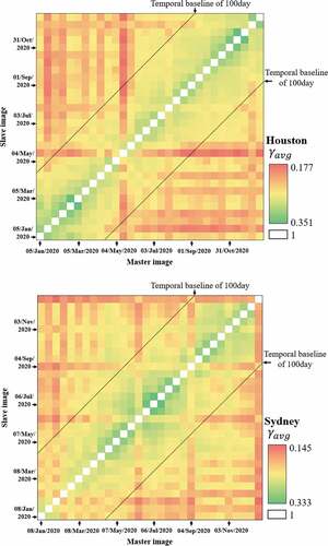When applied using our experimental data, if the baseline is not limited, a total of $30\ast 29/2=435$ interferometric pairs can be formed. The average coherence of all image pairs was then calculated using formula (3), and the average coherence distribution matrices of both study areas are displayed in Figure 2,

Figure 2. Average coherence distribution matrices of the study areas; the black line indicates the temporal baseline of 100 days.

(3) ${\gamma }_{avg}=\frac{\sum _{i=1}^w\sum _{j=1}^l{\gamma }_{(i,j)}}{w\ast l},$(3)

where $w$ and $l$ are the width and length of the image, respectively. ${\gamma }_{i,j}$ is the coherence value at pixel $\left(i,j\right)$.

Each square block in both matrices in Figure 2 represents an interferometric image pair, with its color representing the average coherence. The average coherence between the image and itself is one, that is, the diagonal in each matrix. However, since the interferometry requires two independent images, we did not take into consideration the diagonal in the figure. In general, the shorter the acquisition interval, the better the average coherence of the interferometric pair. A short temporal baseline threshold can guarantee the coherence of the image pairs to some extent. However, there are noticeable outliers, such as Houston data in mid-May, which exhibit poor coherence even between the adjacent images, and the same was found in Sydney’s data in June and September. It was found that the data of spring and winter have a better short-term coherence in both areas: for Houston, it is October to March of the following year, while June to October for Sydney since they lie in different hemispheres.

Assume that the temporal baseline threshold is set at 100 days, that is, the image pairs within the two black lines will be selected to participate in the subsequent deformation inversion process. However, from the average coherence distribution of the two study areas, it was found that many image pairs with poor coherence exist within the set temporal baseline threshold, while the image pairs filtered out by the set threshold also have ones with better coherence.

2.2.3. SBAS-InSAR based on the coherence constraint

The matrix of average coherence exhibits a random distribution that is affected by many factors such as acquisition season, imaging time, and location of the study area. The conventional SBAS-InSAR constraining its baseline with a fixed threshold to ensure better coherence is not applicable in all scenarios. Therefore, we propose to directly use average coherence instead of temporal baseline as a threshold to optimize the combination of image pairs and then carry out the subsequent SBAS-InSAR processing.

For spatial baseline, the height ambiguity of InSAR deformation extraction is $\mathrm{\Delta }{h}_{2\pi }$, that is to say, the interferometric phase changes by 2 π, and the corresponding elevation change is

(4) $\mathrm{\Delta }{h}_{2\pi }=\frac{\lambda Rsin\theta }{2B_{\mathrm{\perp }}},$(4)

where $\lambda$ is the radar echo wavelength, $R$ is the slant range from the radar to the ground pixel, $\theta$ is the incident angle, and $B_{\mathrm{\perp }}$ represents the perpendicular baseline.

In general, when the radar images a certain area, it normally maintains the same position and altitude to ensure the consistency of imaging parameters; therefore, the values of $\lambda ,R,\theta$ are fixed, and the only variable is $B_{\mathrm{\perp }}$, which is inversely proportional to $\mathrm{\Delta }{h}_{2\pi }$. That is to say, the shorter the spatial baseline, the greater the elevation ambiguity and the lower the sensitivity to terrain error. Since the SRTM (Shuttle Radar Topography Mission) DEM (Digital Elevation Model) used for topographic phase removal inevitably contains errors, a shorter spatial baseline can deal with DEM error more effectively. Therefore, on the premise of sufficient data, we first ensured the number of interferometric pairs and then shortened the temporal baseline as much as possible to reduce the impact of DEM error on the accuracy of surface deformation extraction.

After selecting the optimal combination of interferometric pairs by average coherence and spatial baseline thresholds, for any pair, the acquisition time of the master and slave image is assumed to be $t_A$ and $t_B$, respectively. Then, the phase value of a pixel in the $j$ ^th interferometry is obtained after differential interferometry, filtering, and unwrapping process,

(5) ${\phi }_j=\phi (t_B)-\phi (t_A)=\frac{4\pi }{\lambda }[d_{t_B}-d_{t_A}]+\delta {\phi }_j^{topo}+\delta {\phi }_j^{atm}+\delta {\phi }_j^{noise},$(5)

where $\phi \left(t_B\right)$ and $\phi \left(t_A\right)$ are the phase value at $t_B$ and $t_A$. $\delta {\phi }_j^{topo}$, $\delta {\phi }_j^{atm}$, and $\delta {\phi }_j^{noise}$ are the contribution of topographic, atmospheric, and noise phases. The better coherence of interferometric pairs can effectively reduce the impact of the noise phase and thus drives the accuracy up. $d_{t_B}$ and $d_{t_A}$ are the accumulative deformation at $t_B$ and $t_A$ along radar line-of-sight; their difference can be expressed as

(6) $d_{t_B}-d_{t_A}=v_i(t_B-t_A),$(6)

where $v_i$ is the average deformation rate along radar line-of-sight during $t_A$ and $t_B$, in the case of multiple interferometric pairs, and its matrix form can be expressed as

(7) $\mathrm{B}\mathrm{v}=\mathrm{d}\phi .$(7)

Because matrix B is rank-deficient, the singular value decomposition (SVD) method was implemented to obtain the minimum norm solution of the deformation rate, and then the time series deformation was obtained by integrating the velocity in each period.

3. Results and discussion

3.1. Experimental results

We used the proposed method to extract the surface deformation and adopted the results of the conventional SBAS-InSAR as the control group. Baseline combination was performed first. For the conventional SBAS-InSAR approach in study area Houston, 86 interferometric pairs were obtained, given an 80-m spatial baseline threshold and 50-day temporal baseline threshold to bring down the impact of decorrelation and topographic error and yield more accurate results. For the proposed method, we maintained the spatial baseline threshold of 80m and a total of 343 interferometric pairs were formed; then, the first 86 pairs (the same as the control group) with the best average coherence (above 0.23) to perform the following surface deformation extraction are selected. For study area Sydney, similarly, we set a spatial baseline of 100m and a temporal baseline of 70 days for the conventional SBAS-InSAR and acquired 124 interferometric pairs. Then, using the proposed method, we optimized the baseline combination, set a spatial baseline of 100 m, and obtained 404 interferometric pairs, and then the first 124 pairs with the best average coherence (above 0.21) were used for further process. The baseline plots of the two methods in both study areas are shown in Figure 3.

Figure 3. Baseline plots of Common SBAS-InSAR and the proposed method of both study areas.

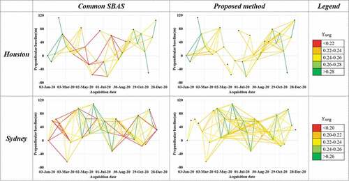
As can be seen from the figure, using fixed temporal baseline threshold in conventional SBAS-InSAR has certain limitations, as it cannot get rid of the interferometric pairs with a short interval but poor average coherence (red baselines), which may introduce decorrelation error in the subsequent processes and affect the accuracy of deformation extraction. The proposed baseline optimization method improved the overall coherence of the selected interferometric pairs, laying a solid foundation for accurate deformation inversion. A histogram of average coherence of the image pairs retrieved by the two approaches was constructed to represent the baseline comparison more clearly, as shown in Figure 4. According to the histogram, the conventional SBAS-InSAR with a fixed temporal baseline introduced a considerable number of pairs with relatively poor coherence in both study areas. However, this phenomenon can be effectively ameliorated by the proposed method. Despite the fact that both methods extracted the same number of pairs with good coherence, the proposed method selected more interferometric pairs in the middle coherence classes, ensuring the overall quality of interferograms and improving the accuracy of deformation inversion.

Figure 4. Histogram comparison of average coherence in Houston (a) and Sydney (b).

To rule out factors other than baselines, the following SBAS-InSAR process was performed utilizing the two types of baselines while keeping other parameters unchanged, including multilook number, filter window size, unwrapping reference point, and threshold value. Figure 5 shows the final deformation rate maps, along with their difference map showing the absolute value of the difference between the two methods.

Figure 5. Deformation rate maps of common SBAS (a) and the proposed method (b) and their difference (c) in Houston (left column) and Sydney (right column).

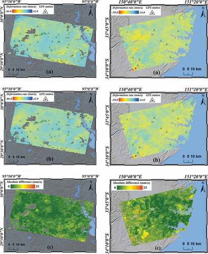
The two approaches had essentially the same deformation trend with some local variances. The maximum subsidence rate in Houston was −86 mm/a, and a large area of decorrelation emerged on the left side of the study area, with a relatively small difference between the two results, while in Sydney, the maximum deformation rate was −59 mm/a, and the overall coherence was better. At the same time, obvious subsidence signs were found in the lower left corner of both deformation maps. The difference between the two results is unevenly distributed, with small differences in the middle and locally large differences up to 20 mm/a on the left side of the study area.

In order to perform quantitative analysis, GPS data from both study areas (also shown in Figure 5) were used as the ground truth (Blewitt, Hammond, and Kreemer 2018), and the deformation rate along line-of-sight retrieved by the two approaches was projected to the vertical direction for comparison. The results are shown in Figure 6, and the standard deviation (STD) of error and root mean square error (RMSE) are selected as the accuracy evaluation indices; their calculation formulas are as follows:

(8) $Std=\sqrt{\frac{1}{n}\sum _{i=1}^n{(e_i-\overline{e_i})}^2},$(8)

(9) $RMSE=\sqrt{\frac{1}{n}\sum _{i=1}^n{(\widehat{y_i}-y_i)}^2}$(9)

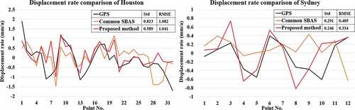
Figure 6. Displacement rate comparison of Houston and Sydney.

where $n$ is the number of points being compared, $e_i$ is the point measurement error, $\overline{e_i}$ is the average error, $\widehat{y_i}$ is the ground truth of GPS, and $y_i$ is the deformation value measured by InSAR.

Figure 6 shows that the deformation rate extracted by the two methods in Houston is very close and is basically consistent with the GPS data. The conventional SBAS approach has a standard deviation of error of 0.813 and an RMSE of 1.082, whereas the proposed method has indices of 0.589 and 1.041, while the two indices of the proposed method are 0.589 and 1.041, respectively. There are only 12 GPS points in study area Sydney, yet when compared to these points, the standard deviation of error of the conventional SBAS method is 0.291 and the RMSE is 0.485, whereas the proposed method’s standard deviation of error is 0.246 and the RMSE is 0.334. The quantitative comparison results show that the proposed method’s deformation extraction results are more accurate than the conventional one, demonstrating the advantage of using the average coherence instead of the temporal baseline as a threshold to optimize the interferometric pair selection and carry out the deformation extraction in the study area.

3.2. Case study of Pingxiang

3.2.1. Study area and data

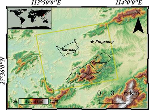
A case study was carried out in Pingxiang, Jiangxi Province, China, to demonstrate the applicability of the proposed method under different scenarios. Pingxiang is located in the west of Jiangxi Province, with copious rainfall and distinct seasons. Inside the study area exist three large coal mines: Anyuan, Gaokeng, and Baiyuan, as shown in Figure 7. Gaokeng and Baiyuan mines were shut down in 2016 and 2020, respectively, due to insufficient production capacity (Fu 2012; He et al. 2017; Liu, Xie, and Mao 2014; Wen et al. 2018). We also used ascending Sentinel-1 SLC data acquired in IW mode with an incidence angle of 36.66° to extract the subsidence of the study area. The spatial resolution after multilooking with a ratio of 5× 1 (range × azimuth) was 20 m. A total of 60 images from January 2019 to December 2020 with an acquisition interval of 12 days were obtained. The images were clipped according to the scope of the study area before further processing, as shown in Figure 7.

Figure 7. Data coverage (yellow rectangle) and boundaries of mines (black lines) in Pingxiang; the background is SRTM DEM.

3.2.2. Baseline combination optimization and experimental results

According to the experimental data, a total of 60 × 59/2 = 1770 interferometric pairs can be obtained if baseline constraints are not set. The average coherence distribution of each pair is shown in Figure 8.

Figure 8. Average coherence distribution matrix of Pingxiang.

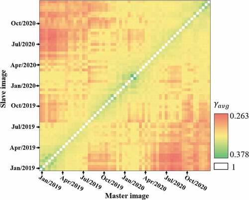
The average coherence distribution of Pingxiang data likewise follows the previous summarized pattern, that is, the shorter the time interval, the better the coherence, and the coherence in spring and winter was higher than that in summer and autumn. At the same time, image pairs with lower coherence (red concentrated area) were not completely distributed in the upper left and lower right corners, where image pairs have the longest acquisition interval. Then, for the baseline combination of conventional SBAS-InSAR, we set a 50-m spatial baseline and 60-day temporal baseline and obtained 119 interferometric pairs; for the proposed method, we set the spatial baseline at 50 m and then combined all the images to get 900 pairs, and then the first 119 pairs with average coherence greater than 0.31 were taken for the subsequent deformation inversion processes. The baseline combination and average coherence distribution of the two methods are depicted in Figure 9 and Figure 10, respectively.

Figure 9. Baseline plots of the proposed and common SBAS-InSAR methods.

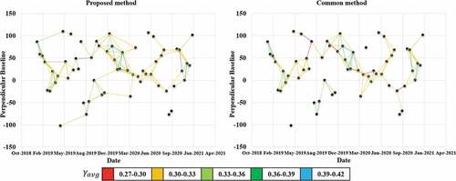
Figure 10. Histogram comparison of average coherence in Pingxiang.

The baseline plots indicate that some pairs (red baseline) with short time intervals but low overall coherence are effectively excluded by the proposed method, so as the isolated image (20,190,412). The histogram reveals that the number of image pairs of the two approaches is consistent in the range of above 0.34, but this portion only accounts for 29.4% of the total. In the columns below 0.34, the difference between the two methods is obvious: for the common SBAS method, there were 16 pairs with the average coherence less than 0.31, accounting for 13.4%, whereas the proposed method extracted no pairs in this section. In the range of 0.31–0.32, the proposed method extracted 32 pairs, 11 pairs more than the common SBAS, and it also extracted more pairs in the rest of the range intervals. Then, the following SBAS-InSAR process was repeated using the two kinds of baselines, respectively, while keeping the other parameters constant, and the final deformation rate maps are presented in Figure 11.

Figure 11. Displacement rate map of the proposed method (left) and common SBAS-InSAR method (right).

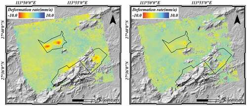
The maximum deformation rate extracted using both approaches all reached −10 mm/a, and distinctive subsidence signs are observed over the mining area. There are two obvious subsidence funnels in the middle of the deformation map extracted by the proposed method. These funnels are typical surface subsidence phenomena induced by underground mining activities, and the entire study area was partially uplifted as a result of intense urban expansion and infrastructure construction. On the other hand, the deformation extracted by the conventional method was more randomly distributed, with more existing null values, and the subsidence funnel was not obvious. On the premise of the same processing parameters, the poor coherence of interferometric pairs of the common SBAS-InSAR is considered to be blamed.

To evaluate the accuracy of the results, five leveling point (shown in Figure 12) data were collected. However, these points are concentrated in Baiyuan coal mine and very close to each other, which may not fully represent the performance over the entire study area if used as ground truth. Since the study area is primarily an urban area with densely distributed permanent scatterers, which is advantageous for PS-InSAR (Ferretti, Prati, and Rocca 1999; Hooper, Segall, and Zebker 2007; Rosi et al. 2018), we used the PS-InSAR results at some permanent scatterers with a coherence above 0.9 as ground truth as some existing literature studies did (Murgia et al. 2019; Li et al. 2020; He et al. 2021), along with the leveling data to perform a validation analysis, and the result is shown in Figure 12.

Figure 12. PS-InSAR and leveling points distribution (upper) and comparison of the methods (lower).

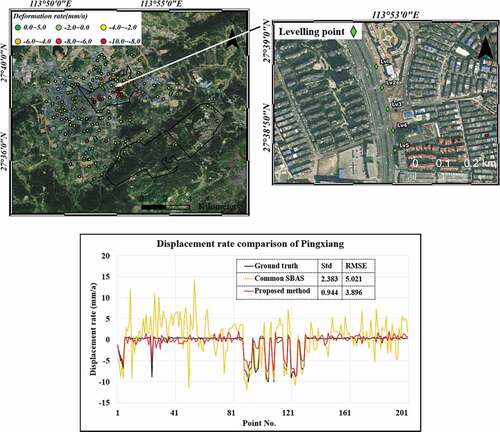
The optical map shows that the study area is mainly located in urban areas, where a significant number of point targets with high coherence are distributed, which is particularly conducive to the deformation inversion of PS-InSAR, and its accuracy can be guaranteed. Compared with the results of PS-InSAR, both the STD of error and RMSE of the proposed method are better than the common SBAS-InSAR approach, proving that the proposed method can extract the surface deformation more accurately.

3.2.3. Deformation time series analysis

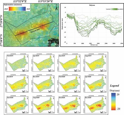
The surface of Baiyuan coal mine corresponds to a dense built-up urban region. As shown in Figure 13, the mine was closed in June 2020, yet its surface deformation rate stayed at −10 mm/a from 2019 until the end of 2020, forming two distinct subsidence funnels. The time series deformation accumulations (Figure 13, lower) reveal that the cumulative deformation increased steadily month by month, exhibiting a linear trend. Furthermore, the maximum cumulative deformation at the section line during two years reached nearly −20 mm.

Figure 13. Zoom-in and cross-section of Baiyuan mine (upper) and its displacement accumulation (lower).

The other two mining sites, Anyuan and Gaokeng, located in the lower part of the study area, are mostly hilly areas with extensive canopy coverage, and the low coherence resulted in serious decorrelation. However, based on the current results, there is a significant subsidence area in the northern part of Anyuan coal mine. If comprehensive analysis and research on the subsidence caused by the ongoing mining activities of Anyuan mine were to be made, longer wavelength radar data are needed to improve the coherence and more effectively extract the subsidence in such densely vegetated areas.

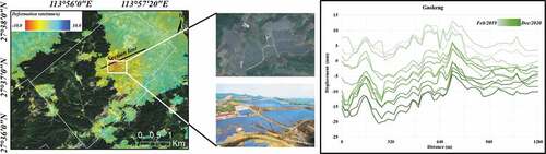
Although the Gaokeng mine was shut down in 2016, it is still subsiding in 2019 and 2020, with an annual deformation rate of −10 mm/a, as illustrated in Figure 14. This is also why even if the mine is closed, the continuous monitoring of its surface deformation is still needed. The right side of the mine is the built-up area, while the left part is the vegetated area, yet there exists a noticeable high coherence area, which is a photovoltaic power station newly built above the original mine site. The solar panels have a high radar reflectivity and operate as a natural reflector, resulting in a high interferometric coherence.

Figure 14. Zoom-in and cross-section of Gaokeng mine.

4. Conclusion

InSAR plays an essential role in surface deformation monitoring. To address the limitation of using a short temporal baseline to ensure the coherence of interferometric pairs in conventional SBAS-InSAR, this paper proposes to directly use the average coherence of interferometric pairs as the thresholding index, rather than a temporal baseline to conduct an optimized selection of interferometric pairs, and then use the selected pairs to extract the surface deformation. Compared with the conventional SBAS-InSAR and GPS data, the STD of error of Houston and Sydney dropped from 0.813 to 0.589 and 0.291 to 0.246, respectively; RMSE decreased from 1.082 to 1.041 and 0.485 to 0.334, respectively, demonstrating the superiority of our method. Following that, a case study was conducted in mining city Pingxiang, China, where obvious surface deformation signals caused by ore mining were discovered, and a time series analysis of surface deformation was carried out to demonstrate the applicability and versatility of the proposed method.

Acknowledgements

The authors would like to thank European Space Agency for providing Sentinel-1A data and NASA for sharing SRTM DEM data. The authors would also like to thank the anonymous reviewers whose comments helped significantly improve this article.

Disclosure statement

The authors declare that they have no known competing financial interests or personal relationships that could have appeared to influence the work reported in this paper.

Data availability statement

The Sentinel-1 SAR data used in the study are available through https://scihub.copernicus.eu/; the SRTM digital elevation model is available through https://srtm.csi.cgiar.org/; and the GPS data are available through http://geodesy.unr.edu/.

Additional information

Funding

This research was funded by Natural Science Foundation of China projects (NSFC) [No: 41801397], National Key R&D Program of China (National Key Research and Development Program of China)[2018YFC0825803].

References

- Ahmed, R., P. Siqueira, S. Hensley, B. Chapman, and K. Bergen. 2011. “A Survey of Temporal Decorrelation from Spaceborne L-Band Repeat-pass InSAR.” Remote Sensing of Environment 115 (11): 2887–2896. doi:10.1016/j.rse.2010.03.017.
- Amelung, F., D. L. Galloway, J. W. Bell, H. A. Zebker, and R. J. Laczniak. 1999. “Sensing the Ups and Downs of Las Vegas: InSAR Reveals Structural Control of Land Subsidence and Aquifer-system Deformation.” Geology 27 (6): 483–486. doi:10.1130/0091-7613(1999)027<0483:STUADO>2.3.CO;2.
- Bateson, L., F. Cigna, D. Boon, and A. Sowter. 2015. “The Application of the Intermittent SBAS (ISBAS) InSAR Method to the South Wales Coalfield, UK.” International Journal of Applied Earth Observation and Geoinformation 34 (1): 249–257. doi:10.1016/j.jag.2014.08.018.
- Berardino, P., G. Fornaro, R. Lanari, and E. Sansosti. 2002. “A New Algorithm for Surface Deformation Monitoring Based on Small Baseline Differential SAR Interferograms.” IEEE Transactions on Geoscience and Remote Sensing 40 (11): 2375–2383. doi:10.1109/TGRS.2002.803792.
- Blewitt, G., W. C. Hammond, and C. Kreemer. 2018. “Harnessing the GPS Data Explosion for Interdisciplinary Science.” Eos 99. doi:10.1029/2018EO104623.
- Bürgmann, R., P. A. Rosen, and E. J. Fielding. 2000. “Synthetic Aperture Radar Interferometry to Measure Earth’s Surface Topography and Its Deformation.” Annual Review of Earth & Planetary Sciences 28 (1): 169–209. doi:10.1146/annurev.earth.28.1.169.
- Chaabani, C., M. Chini, R. Abdelfattah, R. Hostache, and K. Chokmani. 2018. “Flood Mapping in a Complex Environment Using Bistatic TanDEM-X/TerraSAR-X InSAR Coherence.” Remote Sensing 10 (12): 1873. doi:10.3390/rs10121873.
- Chaussard, E., F. Amelung, H. Abidin, and S. H. Hong. 2013. “Sinking Cities in Indonesia: ALOS PALSAR Detects Rapid Subsidence Due to Groundwater and Gas Extraction.” Remote Sensing of Environment 128: 150–161. doi:10.1016/j.rse.2012.10.015.
- Chaussard, E., S. Wdowinski, E. Cabral-Cano, and F. Amelung. 2014. “Land Subsidence in Central Mexico Detected by ALOS InSAR Time-series.” Remote Sensing of Environment 140: 94–106. doi:10.1016/j.rse.2013.08.038.
- Chini, M., R. Pelich, L. Pulvirenti, N. Pierdicca, R. Hostache, and P. Matgen. 2019. “Sentinel-1 InSAR Coherence to Detect Floodwater in Urban Areas: Houston and Hurricane Harvey as a Test Case.” Remote Sensing 11: 107. doi:10.3390/rs11020107.
- Cigna, F., and D. Tapete. 2021. “Present-day Land Subsidence Rates, Surface Faulting Hazard and Risk in Mexico City with 2014–2020 Sentinel-1 IW InSAR.” Remote Sensing of Environment 253: 112161. doi:10.1016/j.rse.2020.112161.
- Dinar, A., E. Esteban, E. Calvo, G. Herrera, P. Teatini, R. Tomás, Y. Li, P. Ezquerro, and J. Albiac. 2021. “We Lose Ground: Global Assessment of Land Subsidence Impact Extent.” Science of the Total Environment 786: 147415. doi:10.1016/j.scitotenv.2021.147415.
- Dong, S., S. Samsonov, H. Yin, S. Ye, and Y. Cao. 2014. “Time-series Analysis of Subsidence Associated with Rapid Urbanization in Shanghai, China Measured with SBAS InSAR Method.” Environmental Earth Sciences 72 (3): 677–691. doi:10.1007/s12665-013-2990-y.
- Ferretti, A., C. Prati, and F. Rocca. 1999. “Permanent Scatterers in SAR Interferometry.” IEEE International Geoscience and Remote Sensing Symposium 3: 1528–1530.
- Fu, Z. 2012. “Research on Transition of China’s Resource Cities: A Case Study of Pingxiang.” Chinese Management Studies 6 (1): 184–203. doi:10.1108/17506141211213988.
- Fujiwara, S., P. A. Rosen, M. Tobita, and M. Murakami. 1998. “Crustal Deformation Measurements Using Repeat‐pass JERS 1 Synthetic Aperture Radar Interferometry near the Izu Peninsula, Japan.” Journal of Geophysical Research: Solid Earth 103: 2411–2426. doi:10.1029/97JB02382.
- Galloway, D. L., and T. J. Burbey. 2011. “Review: Regional Land Subsidence Accompanying Groundwater Extraction.” Hydrogeology Journal 19 (8): 1459–1486. doi:10.1007/s10040-011-0775-5.
- Gatelli, F., A. M. Guamieri, F. Parizzi, P. Pasquali, C. Prati, and F. Rocca. 1994. “The Wavenumber Shift in SAR Interferometry.” IEEE Transactions on Geoscience and Remote Sensing 31: 855–865. doi:10.1109/36.298013.
- He, S. Y., J. Lee, T. Zhou, and D. Wu. 2017. “Shrinking Cities and Resource-based Economy: The Economic Restructuring in China’s Mining Cities.” Cities 60: 75–83. doi:10.1016/j.cities.2016.07.009.
- He, Y., Y. Chen, W. Wang, H. Yan, L. Zhang, and T. Liu. 2021. “TS-InSAR Analysis for Monitoring Ground Deformation in Lanzhou New District, the Loess Plateau of China, from 2017 to 2019.” Advances in Space Research 67: 1267–1283. doi:10.1016/j.asr.2020.11.004.
- Hong, S., E. Chaussard, F. Amelung, and H. Z. Abidin. 2012. “Sinking Cities in Indonesia: Rapid Subsidence Due to Groundwater and Gas Extraction.” AGU Fall Meeting Abstracts 2012: G51B–1100.
- Hooper, A., P. Segall, and H. Zebker. 2007. “Persistent Scatterer Interferometric Synthetic Aperture Radar for Crustal Deformation Analysis, with Application to Volcán Alcedo, Galápagos.” Journal of Geophysical Research 112 (B7). doi:10.1029/2006JB004763.
- Kim, J. W., Z. Lu, Y. Jia, and C. K. Shum. 2015. “Ground Subsidence in Tucson, Arizona, Monitored by Time-series Analysis Using Multi-sensor InSAR Datasets from 1993 to 2011.” ISPRS Journal of Photogrammetry and Remote Sensing 107: 126–141. doi:10.1016/j.isprsjprs.2015.03.013.
- Li, D., X. Hou, Y. Song, Y. Zhang, and C. Wang. 2020. “Ground Subsidence Analysis in Tianjin (China) Based on Sentinel-1A Data Using MT-InSAR Methods.” Applied Sciences 10: 5514. doi:10.3390/app10165514.
- Li, D., Y. Zhou, and H. Ma. 2000. “Principles and Applications of Interferometry SAR.” Science of Surveying and Mapping 25 (1): 10–12.
- Liu, C. Y., P. Xie, and D. Q. Mao. 2014. “Selection of the Superseded Industries of Resources Recession City: A Case of Pingxiang City.” Scientia Geographica Sinica 34 (2): 192–197.
- Liu, G. 2003. “Mapping of Earth Deformations with Satellite Radar Interferometry: A Study of Its Accuracy and Reliability Performances.” Dissertation, Hong Kong Polytechnic University.
- Ma, G., Q. Zhao, Q. Wang, and M. Liu. 2018. “On the Effects of InSAR Temporal Decorrelation and Its Implications for Land Cover Classification: The Case of the Ocean-reclaimed Lands of the Shanghai Megacity.” Sensors 18 (9): 2939. doi:10.3390/s18092939.
- Malinverni, E. S., D. T. Sandwell, A. N. Tassetti, and L. Cappelletti. 2014. “InSAR Decorrelation to Assess and Prevent Volcanic Risk.” European Journal of Remote Sensing 47 (1): 537–556. doi:10.5721/EuJRS20144730.
- Massonnet, D., and K. L. Feigl. 1998. “Radar Interferometry and Its Application Changes in the Earth’s Surface.” Reviews of Geophysics 36 (4): 441–494. doi:10.1029/97RG03139.
- Mohammadimanesh, F., B. Salehi, M. Mahdianpari, J. English, J. Chamberland, and P. J. Alasset. 2019. “Monitoring Surface Changes in Discontinuous Permafrost Terrain Using Small Baseline SAR Interferometry, Object-based Classification, and Geological Features: A Case Study from Mayo, Yukon Territory, Canada.” GIScience & Remote Sensing 56 (3–4): 485–510. doi:10.1080/15481603.2018.1513444.
- Muhammad, S., and L. Tian. 2020. “Mass Balance and a Glacier Surge of Guliya Ice Cap in the Western Kunlun Shan between 2005 and 2015.” Remote Sensing of Environment 244: 111832. doi:10.1016/j.rse.2020.111832.
- Murgia, F., C. Bignami, C. A. Brunori, C. Tolomei, and L. Pizzimenti. 2019. “Ground Deformations Controlled by Hidden Faults: Multi-Frequency and Multitemporal InSAR Techniques for Urban Hazard Monitoring.” Remote Sensing 11: 2246. doi:10.3390/rs11192246.
- Rosi, A., V. Tofani, L. Tanteri, C. Tacconi Stefanelli, A. Agostini, F. Catani, and N. Casagli. 2018. “The New Landslide Inventory of Tuscany (Italy) Updated with Ps-insar: Geomorphological Features and Landslide Distribution.” Landslides 15 (1): 5–19. doi:10.1007/s10346-017-0861-4.
- Syvitski, J. P., A. J. Kettner, I. Overeem, E. W. Hutton, M. T. Hannon, G. R. Brakenridge, J. Day, et al. 2009. “Sinking Deltas Due to Human Activities.” Nature Geoscience 2 (10): 681–686. doi:10.1038/ngeo629.
- Tian, L., T. Yao, Y. Gao, L. Thompson, E. Mosley-Thompson, S. Muhammad, J. Zong, C. Wang, S. Jin, and Z. Li. 2017. “Two Glaciers Collapse in Western Tibet.” Journal of Glaciology 63 (237): 194–197. doi:10.1017/jog.2016.122.
- Tizzani, P., P. Berardino, F. Casu, P. Euillades, M. Manzo, G. P. Ricciardi, G. Zeni, and R. Lanari. 2007. “Surface Deformation of Long Valley Caldera and Mono Basin, California, Investigated with the SBAS-InSAR Approach.” Remote Sensing of Environment 108 (3): 277–289. doi:10.1016/j.rse.2006.11.015.
- Touzi, R., A. Lopes, J. Bruniquel, and P. W. Vachon. 1999. “Coherence Estimation for SAR Imagery.” IEEE Transactions on Geoscience and Remote Sensing 37 (1): 135–149. doi:10.1109/36.739146.
- Van der Sanden, J. J., N. H. Short, and H. Drouin. 2018. “InSAR Coherence for Automated Lake Ice Extent Mapping: TanDEM-X Bistatic and Pursuit Monostatic Results.” International Journal of Applied Earth Observation and Geoinformation 73: 605–615. doi:10.1016/j.jag.2018.08.009.
- Wang, S., X. Lu, Z. Chen, G. Zhang, T. Ma, P. Jia, and B. Li. 2020. “Evaluating the Feasibility of Illegal Open-pit Mining Identification Using Insar Coherence.” Remote Sensing 12 (3): 367. doi:10.3390/rs12030367.
- Wen, B., Y. Pan, Y. Zhang, J. Liu, and X. Min. 2018. “Does the Exhaustion of Resources Drive Land Use Changes? Evidence from the Influence of Coal Resources-exhaustion on Coal Resources–based Industry Land Use Changes.” Sustainability 10: 2698. doi:10.3390/su10082698.
- Wright, P., and R. Stow. 1999. “Detection Mining Subsidence from Space.” International Journal of Remoting Sensing 20 (6): 1183–1188. doi:10.1080/014311699212939.
- Xu, B., G. Feng, Z. Li, Q. Wang, C. Wang, and R. Xie. 2016. “Coastal Subsidence Monitoring Associated with Land Reclamation Using the Point Target Based SBAS-InSAR Method: A Case Study of Shenzhen, China.” Remote Sensing 8: 652. doi:10.3390/rs8080652.
- Zebker, H. A., P. A. Rosen, and S. Hensley. 1997. “Atmospheric Effects in Interferometric Synthetic Aperture Radar Surface Deformation and Topographic Maps.” Journal of Geophysical Research 102: 7547–7563. doi:10.1029/96JB03804.
- Zebker, H. A., and J. Villasenor. 1992. “Decorrelation in Interferometric Radar Echoes.” IEEE Transactions on Geoscience and Remote Sensing 30: 950–959. doi:10.1109/36.175330.
- Zhao, C., Z. Lu, Q. Zhang, and J. de La Fuente. 2012. “Large-area Landslide Detection and Monitoring with ALOS/PALSAR Imagery Data over Northern California and Southern Oregon, USA.” Remote Sensing of Environment 124: 348–359. doi:10.1016/j.rse.2012.05.025.
- Zhao, R., Z. W. Li, G. C. Feng, Q. J. Wang, and J. Hu. 2016. “Monitoring Surface Deformation over Permafrost with an Improved SBAS-InSAR Algorithm: With Emphasis on Climatic Factors Modeling.” Remote Sensing of Environment 184C: 276–287. doi:10.1016/j.rse.2016.07.019.
- Zhou, L., J. Guo, J. Hu, J. Li, Y. Xu, Y. Pan, and M. Shi. 2017. “Wuhan Surface Subsidence Analysis in 2015–2016 Based on Sentinel-1A Data by SBAS-InSAR.” Remote Sensing 9: 982. doi:10.3390/rs9100982.