Solar park detection from publicly available satellite imagery

ABSTRACT

The rapid increase in large-scale photovoltaic installations, or solar parks, causes a need to monitor their amount and allocation, and assess their impacts. While their spectral signature suggests that solar parks can be identified among other land covers, this detection is challenged by their low occurrence. Here, we develop an object-based random forest (RF) classification approach, using publicly available satellite imagery, which has the advantage of requiring relatively little training data and being easily extendable to large spatial extents and new areas. First, we segmented Sentinel-2 imagery into homogenous objects using a Simple Non-Iterative Clustering algorithm in Google Earth Engine. Thereafter, we calculated for each object the mean, standard deviation, and median for all 10- and 20-meter resolution bands of Sentinel-1 and Sentinel-2. These features are subsequently used to train and validate a range of RF models to select the most promising model setup. The training datasets consisted of subsampled presence/absence data, oversampled presence/absence data, and multiple land-cover categories. The best-performing model used an oversampled dataset trained on all 10- and 20- meter resolution spectral bands and the radar backscatter properties of one period. Independent test results show an overall classification accuracy of 99.97% (Kappa: 0.90). For this result, the producer accuracy was 85.86% for solar park objects and 99.999% for non-solar park objects. The user accuracy was 92.39% for solar park objects and 99.999% for non-solar park objects. These high classification accuracies indicate that our approach is suitable for transfer learning and is able to detect solar parks in new study areas.

KEYWORDS:

• Photovoltaics
• object-based image classification
• random forest
• transfer learning
• land use
• land cover

1. Introduction

Renewable energy sources, including solar power, hydropower, wind power, biomass and geothermal energy, are necessary to decarbonize the energy sector and avoid the worst impacts of climate change (IPCC 2014; Trappey et al. 2016). Over the past few years solar photovoltaics (PVs) installation has increased rapidly, mainly due to the reduction of costs and strong policy support in Europe, the United States, Japan, China, and India (Haegel et al. 2017; International Energy Agency 2021). The International Energy Agency (2021) estimated that the global solar PV energy generation increased from 665 TWh to 821 TWh in 2020 alone. This is an increase of 23% in only one year, and as a result, the share of PVs in global electricity generation is approaching 3.1%. Solar PV panels are installed as rooftop panels, as floating PV plants on lakes, canals and offshore sites, and as “solar parks,” which are large-scale PV installations (Sahu, Yadav, and Sudhakar 2016). In contrast to rooftop systems and floating PV plants, solar parks generate power at the utility level and have ground-mounted PV panels (Kok et al. 2017). These PV panels are distanced from each other, to avoid the cast of shadows onto a panel (RVO and ROM3D 2016; ROM3D 2021).

Mapping solar parks is important in order to quantify the amount of renewable energy that is produced as well as to assess the potentially negative impact on their immediate environment. Although solar parks have the advantage of generating renewable energy (Tsoutsos, Frantzeskaki, and Gekas 2005), they are also associated with soil degradation due to extensive landscape modifications, potential losses of biodiversity and habitats, as well as landscape fragmentation (Hernandez et al. 2014). Solar panels affect local soil conditions by reducing the amount of sunlight and water reaching the soil and vegetation (Frambach and Schurer 2019; Kok et al. 2017). Besides, solar parks decrease surface temperatures, due to enhanced effective albedo, solar panel shading, and convection cooling of PV installations (Zhang and Xu 2020). Furthermore, several studies indicate that solar parks have negative esthetic impacts on the surrounding landscape (Sánchez-Pantoja, Vidal, and Carmen Pastor 2018; Del Carmen Torres-sibille et al. 2009). Lastly, solar parks tend to cover large areas and they therefore compete with agriculture or nature for scarce land (van der Zee et al. 2019). For these reasons, it is important to track the locations and development of solar parks. However, only few countries have spatially explicit national data about solar PVs locations, and these are often not open access (Dunnett et al. 2020). Besides, solar databases, like Wiki-Solar, are not complete (Scott, Brown, and Culbertson 2019) as they depend on voluntary contributions. Therefore, there is a need to map large-scale PV installations to quantify and optimize the efficiency of solar panels, and assess their environmental impacts (Hou et al. 2019)

Satellite imagery offers an alternative for identifying solar parks at large spatial scales and with a high level of detail. We hypothesize that PVs are sufficiently distinct from other landscape features to detect them using publicly available imagery in machine learning algorithms, such as random forest classifiers (RF) and convolutional neural networks (CNN) (Phan, Kuch, and Lehnert 2020; T. Zhang et al. 2021). CNNs are deep learning networks that can classify and segment images by learning spectral and spatial relations from the input data (Arel, Rose, and Karnowski 2010), in contrast to RF classifiers. The disadvantage is that a CNN generally require large datasets for training. We chose a RF in this study, because it requires less training data, is more robust against noise and the setup is simple compared to other non-parametric methods (Rodriguez-Galiano et al. 2012).

lthough satellite and aerial imagery in combination with machine learning algorithms have widely been used to identify a variety of objects, such as buildings, roads and ships (e.g. Alshehhi et al. 2017; Li et al. 2021), very few studies identified solar parks. Previous studies trained CNNs based on hyperspectral imagery to map PVs as solar parks (Hou et al. 2019) and as panels on roofs of residential buildings (e.g. Castello et al. 2019; Yu et al. 2018; Yuan et al. 2016; Malof et al. 2015). However, these studies depend on very-high resolution imagery (<1 m spatial resolution), which is resource-intensive and constrains the application over large spatial extents. The study by da Costa et al. (2021), in contrast, utilized multi-spectral Sentinel-2 imagery to detect and segment solar parks with high accuracies. The aim of this study is to develop and test a classification approach that is able to detect solar parks at large spatial scales and that uses only publicly available satellite imagery. Specifically, we trained RF models in an Object-Based Image Analysis (OBIA) approach using different combinations of multispectral Sentinel-2 imagery, and radar backscatter from SAR (Synthetic Aperture Radar) imagery of Sentinel-1. These datasets were selected based on the properties in which solar parks can be distinguished from other land cover categories. By using the Google Earth Engine (GEE) both to preprocess the data, and to create segments for the OBIA we present an approach that is not reliant on heavy computational resources. We tested a wide range of model specifications to find the optimal set of data for the detection of solar parks and subsequently examined the model’s capacity to transfer learning.

2. Materials and methods

2.1 Overall approach and case study area

This study combines two procedures to identify solar park objects: image segmentation and random forest classification (RF). Image segmentation divides an image into relatively homogenous objects (segments) based on spectral characteristics of adjacent pixels. Segmentation yields a uniform and homogeneous object according to some characteristics, for example color, texture, or height (Haralick and Shapiro 1985), which can be used as input to OBIA. Each object, consisting of one or more pixels, is subsequently classified based on its feature characteristics (Liu and Xia 2010). We chose OBIA over pixel-based classification because this removes the so-called salt-and-pepper effect as well as reduces the spectral variation of PV installations (Liu and Xia 2010).

An RF classifier consists of a group of decision trees, where each tree is constructed by randomly taking a bootstrap sample from the original dataset. Each tree consists of multiple nodes. At each node, a subset of randomly selected features, for instance spectral information, is created. The eventual classification of an object depends on the majority outcome of all trees (Breiman 2001).

We trained RF models with different combinations of satellite imagery to determine whether objects in the Netherlands are solar parks or not. Figure 1 provides an overview of our methodology. We tested our approach to detect solar parks in the Netherlands because the location of all solar parks in the Netherlands is known, and the number of solar parks is sufficiently high for a reliable accuracy assessment. Solar parks in the Netherlands are located in industrial and business parks and agricultural areas. As of 2020, 135 solar parks were realized with an average area of 6615 m² (std. 2207.39 m²) (ROM3D 2021).

Figure 1. Methodological approach of this study. Orange parallelepipeds indicate input remote sensing data; yellow boxes symbolize processing steps and red parallelepipeds indicate input data for the random forests. Light blue ovals symbolize the intermediate results and the blue oval indicate the end result.

2.2 Image segmentation and ground truth data

We used the Simple Non-Iterative Clustering (SNIC) segmentation to identify objects as input for our classification algorithm (Achanta and Süsstrunk 2017). Mahdianpari et al. (2019) showed that SNIC is suitable for the segmentation of Sentinel-2 data and that it is superior in processing time to comparable methods thanks to the use of 4- or 8-connected pixels. The implementation of SNIC in GEE has the added benefit that no computational resources are necessary for users. The algorithm starts with centroids, which are a uniform grid of pixels. Around the centroids, clusters of pixels, called super-pixels, are formed using a distance calculation in a five-dimensional space of color and spatial coordinates. The distance calculation combines normalized spatial and color distances. The SNIC requires two user-defined parameters: (1) object size and (2) object compactness that controls the possible geometry of an object. The compactness and boundary continuity exhibit a trade-off, as a larger compactness results in more compact super-pixels and poor boundary continuity. To select the next pixels to join the cluster, the SNIC uses 4- or 8-connected candidate pixels in the growing super-pixel. The candidate pixel is selected based on the smallest distance from the centroid. In this study, the required parameters were manually set, and the results were visually inspected to further refine the parameter settings. The parameters included: (1) compactness, which was set to 1; (2) connectivity, which was set to 4; (3) neighborhood size, which was set to 64; (4) size, which was set to 10; (5) seeds, which was set to 15; (6) kernel, which was set to 3; and (7) scale, which was set to 10.

We randomly gathered SNIC-segmented objects for all land categories in the northern part of the Netherlands, covering the provinces Overijssel, Flevoland, Noord-Holland, Drenthe, Gelderland and Friesland (Figure 2), and used the objects to train RF models. The northern part of the Netherlands is hereafter referred to as “training area.” Validation data was drawn from a region not belonging to the training area, to avoid overfitting and to develop a model that can potentially be applied in new regions (transfer learning). To this end, a validation dataset was created from an area of about 1600km² in Zeeland, Noord-Brabant and Limburg, hereafter referred to “validation area” (Figure 2). Subsequently, to test how well the model is able to generalize, the best performing validation model was used to predict the location of solar parks in an independent test dataset covering the entire province of Groningen (2800km²), hereafter referred to as “test area” (Figure 2).

Figure 2. Study area with the training area (northern part of the Netherlands; blue), the validation areas (Zeeland, Noord-Brabant, Limburg; brown) and the test area (Groningen; green)

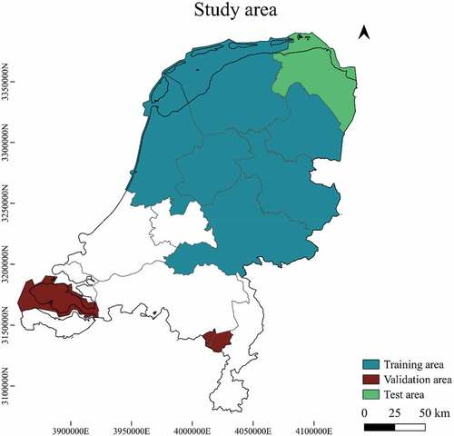
The ground truth location of the solar parks present in 2020 in the training, validation, and test data was derived from the websites http://zonopkaart.nl/, https://www.wiki-solar.org/ and https://www.vallei-veluwe.nl/. We considered panels that stood >10 meters apart from each other as separate solar park arrays. Objects segmented by the SNIC algorithm that existed more than 50% of a solar park were labeled as solar park. In total, 924 polygons covering PV panels in the training dataset were selected. The validation dataset contained 369 polygons with solar parks and the test dataset contained 1341 polygons that represented a solar park.

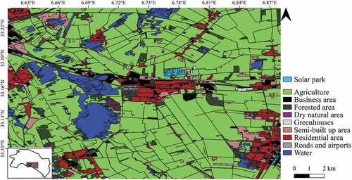
The land-use and land-cover (from here on: land cover) categories we identified in this study were (1) agriculture, (2) business areas, (3) forested areas, (4) dry natural areas, (5) greenhouses, (6) semi-built up areas, which have some degree of paving but are not used as an area for traffic, (7) roads and airports, (8) residential areas, (9) sand, and (10) water. The location of these land cover objects was based on the Bestand Bodemgebruik 2015 (Nationaal Georegister 2018) of the Centraal Bureau van de Statistiek (CBS), downloaded from PDOK.nl. The dataset consisted of geometries/objects of land cover categories. The CBS determined the boundaries of these objects using object-based topographical datasets (TOPNL) and interpreted the land cover with aerial photographs from 2015. A land cover map with the objects covering a part of the test area is shown in Figure A1. In this study, SNIC-segmented objects distributed over the entire research area were selected. Visual inspection with Sentinel-2 imagery from March 2021 determined whether the land cover had not changed compared to the Bestand Bodemgebruik 2015, in which case they were omitted from our datasets.

The total number of objects for each category in the training dataset is tabulated in Table 1. The horizontal length of the PV objects ranged between 12 and 492 meters, and the width ranged between 10 and 263 meters. The average width was 83 meter (std 26 meter), and the average length was 127 meter (std 43 meter).

Table 1. Overview of the objects per land cover category in the training dataset.

Land cover category	Area Mean (m^2)	Std. (m^2)	Number of objects
Solar park	6615	2207	924
Agriculture	6890	1639	867
Business area	6043	3065	870
Forested area	6694	1429	870
Dry natural area	6182	1479	863
Greenhouses	6784	2320	865
Sand	9286	1827	1014
Semi-built up area	6372	2533	841
Residential area	7624	2072	863
Roads and airports	7052	2307	863
Water	6819	1646	846
Total			9686

2.3 Satellite imagery

We trained and applied our RF model using satellite imagery from various publicly available sources. Specifically, we used spectral information from Sentinel-2, and SAR data from Sentinel-1. A description of the datasets and derived products that we used is shown in Table 2, and further detailed below.

Table 2. Satellite imagery used in this study.

Imagery	Tile	Acquisition dates	Spectral bands	Spatial resolution
Sentinel-2	31UES	19–09-2020; 31–03-2021	Blue (Band 2, 490 nm); Green (Band 3, 560 nm); Red (Band 4, 665 nm); Near Infrared (Band 8, 842 nm);   Red edge 1 (Band 5, 704 nm);Red edge 2 (Band 6,740 nm); Red edge 3 (Band 7, 783 nm); Narrow Near Infrared (Band 8a, 865 nm);   SWIR 1 (Band 11, 1614 nm); SWIR 2 (Band 12, 2202 nm)	10 m; 20 m
	31UET	22–09-2020; 31–03-2021
	31UEU	22–09-2020; 31–03-2021
	31UFS	22–09-2020; 31–03-2021
	31UFT	22–09-2020; 31–03-2021
	31UFU	22–09-2020; 31–03-2021
	31UFV	22–09-2020; 31–03-2021
	31UGS	22–09-2020; 31–03-2021
	31UGT	22–09-2020; 31–03-2021
	31UGU	22–09-2020; 31–03-2021
	31UGV	22–09-2020; 31–03-2021
	32ULB	22–09-2020; 31–03-2021
	32ULC	22–09-2020; 31–03-2021
	32ULD	22–09-2020; 31–03-2021
	32ULE	22–09-2020; 31–03-2021
Sentinel-1	-	1/09/2020 – 30/09/2020; 31/03/2021 – 04/04/2021	VV and VH polarization	10 m

2.3.1 Sentinel-2 imagery

We used Sentinel-2 imagery to extract spectral information of the solar parks and other land cover categories. Sentinel-2 imagery has already been used in previous studies for various land monitoring applications, such as mapping built-up areas (Pesaresi et al. 2016) and land-cover classifications (Phan, Kuch, and Lehnert 2020), indicating a high potential of Sentinel-2 imagery for such applications. In this study, we used the 10-meter resolution bands, i.e. the blue (band 2, 490 nm), the green (band 3, 560 nm), the red (band 4, 665 nm), and the NIR (band 8, 842 nm). PV panels have a relatively low reflectance in the visible and near-infrared portion of the spectrum, due to the characteristics of which the panels are composed (Czirjak 2017).

We also included the 20-meter resolution bands, which consists of the red edge 1 (Band 5, 704 nm), red edge 2 (Band 6,740 nm), red edge 3 (Band 7, 783 nm), the narrow NIR (band 8a, 865 nm), the SWIR 1 (band 11, 1614 nm), and the SWIR 2 (band 12, 2202 nm). We added the different red edge bands and the narrow NIR, as they are useful to estimate the state of vegetation and can therefore be used to differentiate between vegetated and non-vegetated areas (Sun et al. 2021). The SWIR bands were included, as they have previously been used to identify minerals and bare soils (Yamaguchi and Naito 2003). We used Sentinel-2 imagery from spring (March 2021) and autumn (September 2020), because multi-temporal imagery tends to improve the differentiation between vegetation and non-vegetation, as the spectral reflectance of for instance forests and crops changes between seasons (Song, Woodcock, and Xiaowen 2002).

The Normalized Difference Vegetation Index (NDVI) was also included. This was calculated from the Sentinel-2 data using the following formula

(1)

The NDVI was used to determine if areas contain vegetation, which is useful to differentiate between vegetated areas and non-vegetated areas such as solar parks (Defries and Townshend 1994). Furthermore, the Normalized Difference Water Index (NDWI) was also added and can be used to detect water bodies (McFeeters 1996). The NDWI is calculated with the following formula:

(2)

Sentinel-2 tiles (Table 2) covering the Netherlands were obtained from GEE. The selection criteria for the images were <1% cloud cover and an acquisition period in or close to September 2020 and March 2021. The GEE data are atmospherically corrected Sentinel-2 imagery at level-2A.

2.3.2 Sentinel-1 imagery

We used SAR data, as we expected the surface roughness of the PV panels differs from other land covers such as buildings or trees. In order to utilize the different radar backscatter properties of each land cover category, Sentinel-1 imagery was used. Sentinel-1 collects C-band (5.407 GHz) SAR imagery at a 10 m resolution and at a variety of polarizations and resolutions during ascending and descending orbits. The system operates in different acquisition modes: Stripmap, Interferometric Wide swath (IW), Extra-Wide swath, and Wave. The IW is the default mode over land. The geometric plane in which the radar waveis transmitted and received is referred to as polarization, which is either horizontal (H) or vertical (V) in respective to the satellite antenna. Previous studies used Sentinel-1 imagery for various applications; for example the VV and VH have previously been used to estimate building heights (Frantz et al. 2021; M. Li et al. 2020) and to detect water bodies (Pham-Duc, Prigent, and Aires 2017; Clement, Kilsby, and Moore 2018).

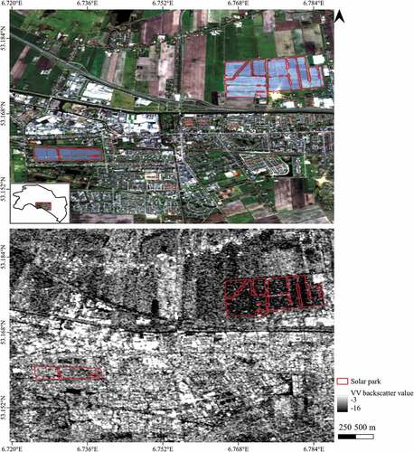
GEE offers calibrated, ortho-corrected Sentinel-1 imagery with a spatial resolution of 10 m. This imagery was pre-processed by thermal noise removal, radiometric calibration, and terrain correction, as implemented by the Sentinel-1 toolbox (ESA 2020). For this study, the VV and VH in the IW mode from 23 until 27 March 2021 were used from both the descending and ascending orbits. The VV raster-imagery from March 2021 covering a part of the test area is shown in Figure 3. This figure shows that built-up areas have high backscatter intensity, and waterbodies have low backscatter intensities compared to solar parks.

Figure 3. RGB Sentinel-2 imagery showing a part of the test area with the location of solar park panels on top. Backscatter imagery of the VV mode from March 2021 in the bottom.

2.4 Data processing

To detect solar parks, we fed an RF model with different combinations of the abovementioned datasets. For each of the segmented objects, the surface spectral reflectance from the 10- and 20-meter Sentinel-2 resolution bands and the VV and VH backscatter values from the Sentinel-1 images were extracted. For each feature, we calculated the mean, standard deviation, and median to account for the potential influence of weather or pollution. We augmented each object in the training dataset three times by randomly changing the brightness to enlarge the training dataset size and account for atmospheric changes. The brightness values were randomly changed within a factor range of [−0.2, 0.2], similar to the approach of Knopp et al. (2020). After the augmentation, the training dataset consisted of 38744 objects.

The extracted satellite data were used as explanatory variables in the RF models. These models were trained with the R-package randomForest (version 4.6–14) (Liaw and Wiener 2002). We trained various models using different combinations of training sample size (e.g. subsampled or oversampled) and explanatory variables (only the Sentinel-2 bands, or the Sentinel-2 bands combined with the Sentinel-1 backscatter information), to assess the impact on the classification accuracies of the validation dataset. Subsequently, the RF model with the best validation results was used to classify objects in the test dataset. In order to reduce the amount of false positives caused by any small objects being erroneously classified as PV installation, we filtered the objects that were classified as solar parks based on the surface area of the smallest solar park object in the training data. The filter threshold was set to 1034.7 m². Ultimately, we created a map with the predicted location of solar parks in Groningen.

2.5 Experimental set-up

We applied a classification based on the label of the land cover categories (e.g. solar park, agricultural area, or forested area) and a classification based on a yes/no label (indicating only whether an object is a solar park or not). Regardless of the labeling, classification accuracies of the validation and test dataset indicate the accuracy of separating the solar park from no solar park objects. We considered solar panels on rooftops that were detected by the model as PV panels as true positives, even though we did not train the model using rooftop solar panels.

The RF model requires two initialization parameters: (1) the number of classification trees or bootstrap iterations (ntree), and (2) the number of input variables randomly split at each node (mtry). The default settings for mtry and ntree were applied in this study, where the value for mtry is √p and p stands for the number of predictor variables in a dataset (Liaw and Wiener 2002), and ntree = 500. The explanatory power of the input data was calculated by the mean decrease in accuracy (MDA) and the mean decrease in Gini (MDG). The MDA expresses how much the accuracy of a model is lowered by excluding a variable and the MDG indicates how each variable contributes to the homogeneity of the nodes and leaves in the RF model.

We balanced the amount of samples per category in the training dataset, because classification algorithms aim to minimize the overall error rate and to maximize the overall classification accuracies. Consequently, the algorithm tends to fit the model to the majority class, in this case, the no solar park category (Chen, Liaw, and Breiman 2004). Specifically, we trained the model on an oversampled yes/no dataset, a subsampled yes/no dataset, and on all datasets including all land cover classes separately (Table 3). For the subsampled dataset, we reduced the amount of samples for each class until the total amount of non-PV equaled the amount of PV samples. For the oversampled dataset, we randomly oversampled the PV category by randomly duplicating solar park objects, while the original data remained intact (Kuhn 2021). For the model trained on all land cover classes, we used all actual training data without further adjustments.

Table 3. The number of objects in the oversampled, subsampled, and land cover categories training datasets, after data augmentation.

Set	Yes/No category	Land cover category	n (Train model)
Oversampled training data	Solar park	-	35,048
	No solar park		35,048
Subsampled training data	Solar park	-	3696
	No solar park		3702
Land cover categories	-	Solar park	3696
		Agriculture	3468
		Business area	3480
		Forested area	3480
		Dry natural area	3452
		Greenhouses	3460
		Sand	4056
		Semi-built up area	3364
		Residential area	3480
		Roads and airports	3452
		Water	3384

After validation, the model that yielded the best validation accuracies was used to classify the independent test dataset. By doing so, we assessed whether the model is able to generalize and thus further assess its capacity for transfer learning.

2.6 Accuracy assessment

The RF model evaluation used different precision metrics: (1) producer accuracy, representing the probability that a reference sample is correctly identified in the classification map; (2) user accuracy, indicating the probability that a classified object in the classification map accurately represents that category on the ground; (3) overall accuracy (OA), determining the overall efficiency of the algorithm; (4) Kappa, indicating the degree of agreement between the ground truth data and the predicted value corrected for chance agreement; (5) Jaccard-Index (IoU), expressed as the intersection divided by the union of a class in the reference data and the classification result, calculating the similarity and diversity of sample sets; and lastly (6) F-measure, the harmonic mean of precision and recall (Congalton 1991). The F-measure ranges from 0 to 1, with 1 indicating a small amount of false positives and negatives. We used the F-measure value as the metric for the selection of the best performing RF model.

3. Results

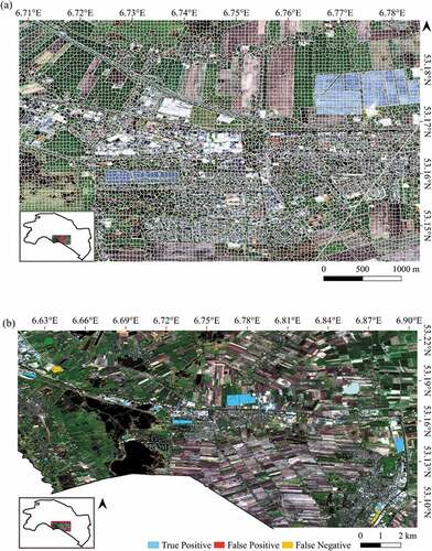
The most accurate model yielded a producer accuracy of 85.86%, a user accuracy of 92.39% and a IoU of 80.19% for detecting solar parks in the test region (F-measure: 0.89). For no solar park objects, the producer accuracy was 99.996%, and the user accuracy was 99.997% (F-measure: 0.99997). The overall accuracy of the test dataset was 99.97% (Kappa: 0.90). Figure 4 shows the object segmentation and the final results in a subsection of our test area. These results are generated with an RF model that was trained on an oversampled dataset using the spring 10- and 20-meter resolution Sentinel-2 imagery in combination with the backscatter Sentinel-1 features from spring (Table 4). This model specification yielded the best validation results and was therefore selected to detect solar parks in the test area. Our model detected 41 PV arrays of 15 solar parks that are not yet present in the databases of http://zonopkaart.nl/ and https://www.wiki-solar.org/. In addition, the model classified objects belonging to PV panels on rooftops as solar park; to be specific, 11 out of 1386 classified PV objects belonged to rooftop PV panels. The accuracy of the independent test is comparable to the accuracy of the validation (producer accuracy 81.39%, user accuracy 92.39%, F-measure of 0.80, see Table 4).

Table 4. Validation results for different RF models trained on datasets with oversampled yes/no categories.

Model	Category	Producer accuracy	User accuracy	F-measure	IoU	Overall accuracy	Kappa
Sentinel-2 (10 m resolution) spring	Solar park	58.88%	6.97%	0.12	6.65%	99.37%	0.55
	No solar park	99.92%	99.997%	0.9996	99.92%
Sentinel-2 (10 m resolution + NDVI) spring	Solar park	58.94%	9.06%	0.16	8.53%	99.57%	0.51
	No solar park	99.92%	99.997%	0.9996	99.92%
Sentinel-2 (10 m resolution + NDWI) spring	Solar park	57.29%	15.05%	0.24	13.53%	99.74%	0.52
	No solar park	99.94%	99.997%	0.9997	99.94%
Sentinel-2 (10 & 20 m resolution) spring	Solar park	80.24%	88.22%	0.84	72.47%	99.99%	0.98
	No solar park	100.00%	99.999%	0.99999	100%
Sentinel-2 (10 & 20 m resolution) spring + Sentinel-1 spring	Solar park	81.39%	92.39%	0.87	76.28%	99.99%	0.99
	No solar park	99.999%	99.999%	0.9999	100%
Sentinel-2 (10 & 20 m resolution) spring & autumn + Sentinel-1 spring	Solar park	96.83%	63.22%	0.76	61.93%	99.95%	0.80
	No solar park	99.99%	99.9996%	0.9999	99.99%
Sentinel-2 (10 & 20 m resolution) spring & autumn + Sentinel-1 spring & autumn	Solar park	96.50%	71.61%	0.82	69.80%	99.97%	0.93
	No solar park	99.99%	99.999%	0.9999	99.99%

The classification accuracies of the validation dataset indicate that the models trained on an oversampled yes/no dataset outperformed the models trained on a subsampled yes/no dataset or the land cover category dataset for all model specifications (Table A2). Interestingly, the model with the highest accuracy when trained with the subsampled data only used the spring 10- and 20-meter resolution Sentinel-2 imagery. This model yields a producer accuracy of 91.96% and a user accuracy of 31.07%. Adding the Sentinel-1 data here results in a higher producer accuracy, but a lower user accuracy, and together this yields a lower F-measure (0.42 versus 0.46).

The classification accuracies for the validation of the model trained on all land cover classes perform better than the subsampled but worse than the oversampled model for all model specifications (Table A1). Similar to the subsampled model, the highest accuracy here is obtained with the model that uses only used the spring 10- and 20-meter resolution Sentinel-2 imagery. For this model, the producer accuracy is 88.56% and the user accuracy is 72.37%, leading to an F-measure of 0.80. By comparison, the model that also includes Sentinel-1 spring data yields an F-measure 0.71 (Table A1).

For all three training datasets, the best classification accuracies were obtained for the models using the 10- and 20-meter resolution bands from Sentinel-2 imagery from one season in combination with and without the VV and VH backscatter properties from Sentinel-1 imagery. In the validation dataset, the best performing model had a producer accuracy of 81.39% and a user accuracy of 92.39% for solar park objects and a producer and user accuracy of 99.999% for no solar objects. The model obtained an overall accuracy of 99.99% (Kappa: 0.99).

The models with the lowest accuracy metrics and statics were the models that only used the green, blue, red and NIR bands. The addition of the NDVI, NDWI, Red edge, SWIR and backscatter information improved the classification results. The addition of the autumn Sentinel-2 and Sentinel-1 imagery had a negative impact on the classification results, since the number of false positives increased, leading to a lower user accuracy.

Figure 4. RGB Sentinel-2 imagery showing a part of the test area. Firstly, Sentinel-2 10 m resolution imagery was segmented with the SNIC algorithm (a). Secondly, the objects were classified with an RF model (b). To facilitate interpretation, true negatives are not shown on the map.

3.2 Variable importance, SHAP-values and ROC curve

The variable importance plot of the best performing model shows the explanatory power of the different input variables (Figure 5). The plot suggests that the SWIR 1 mean and SWIR 1 median, as well as the NDWI mean and median contributed most to the RF model. These variables also had high predictive power. The relevance of SWIR-1 is further illustrated by the spectral reflectance curves, which shows that solar parks are particularly distinct from other land cover categories in this bandwidth (1614 nm) (Figure 6). Additionally, we calculated the mean SHAP-values of the best performing model over all observations, which provides the global feature importance. SHAP-values are used to overcome inconsistencies of traditional variable importance methods. For example, two equally important features in tree-based models are given different values based on what level of splitting was done; the features which split the model first might be given higher importance (Lundberg, Erion, and Lee 2018). The SHAP-variable importance plot (Figure 7) also indicates that the mean and median of SWIR 1 and NDWI contributed most to the models performance.

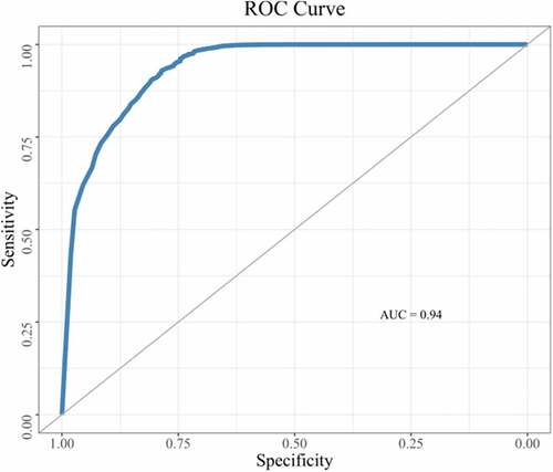
We used the validation dataset to construct a Receiver Operator Characteristic (ROC) curve of the best performing model (Figure 8). The ROC curve represents the trade-off between the sensitivity (true positive rate) and specificity (1- false positive rate). When the ROC curve is closer to the top-left corner, the binary RF classification yields a better performance. The area under the ROC curve (AUC) indicates the model’s ability to distinguish between two classes. The AUC ranges between 0 and 1, where a value of 1 indicates a better model. The AUC of our best performing model was 0.93.

Figure 5. Variable importance plot of the RF model trained on an oversampled dataset and using the 10- and 20-meter resolution (green, blue, red, NIR, NDVI, NDWI, Red edge and SWIR) Sentinel-2 bands in combination with VV and VH backscatter properties from Sentinel-1 imagery as explanatory variables.

Figure 6. Spectral reflectance curves of included land cover categories based on the 10 and 20 m resolution bands of Sentinel-2 imagery from March 2021.

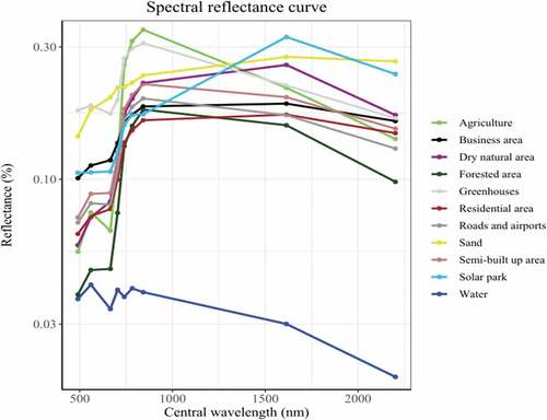
Figure 7. Variable importance plot showing the mean SHAP values over all observations of the RF model trained on an oversampled dataset and using the 10- and 20-meter resolution (green, blue, red, NIR, NDVI, NDWI, Red edge and SWIR) Sentinel-2 bands in combination with VV and VH backscatter properties from Sentinel-1 imagery as explanatory variables.

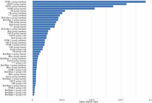
Figure 8. ROC curve of the validation dataset classified by the RF model trained on an oversampled dataset and using the 10- and 20-meter resolution (green, blue, red, NIR, NDVI, NDWI, Red edge and SWIR) Sentinel-2 bands in combination with VV and VH backscatter properties from Sentinel-1 imagery as explanatory variables.

4. Discussion

Our results indicate that a RF model trained on spectral and backscatter features has a high potential to detect automatically segmented solar park objects. We found that the validation models that used an oversampled dataset in the Y/N category outperformed the models trained on subsampled Y/N categories or on multiple land cover categories. By subsampling the training data, objects might have been left out that contain crucial information about a category. As a consequence, the overall accuracy of a model applied to an independent dataset might be lowered (Maxwell, Warner, and Fang 2018)

Furthermore, to assess the added value of the different satellite datasets on the performance of the model, we applied different combinations of the datasets. With the addition of more explanatory features, e.g. the Sentinel-2 and Sentinel-1 images from autumn, the classification results were lowered, as also found by Georganos et al. (2018). Other explanatory features, not considered in this study, can also be used to identify solar parks. The study by Zhang et al. (2021) used the 100 meter resolution bands from the Landsat-8 mission, as the land surface temperature of the solar parks is different from the surroundings (Zhang and Xu 2020). The authors, however, found that the thermal bands had little effect on the accuracy of the model, which they attributed to the coarse resolution of the bands and to the likelihood that surface temperatures of the PV power plants would be more similar to other ground objects over large regions. Besides the thermal information, the study used textural information of power plants to analyze the spatial autocorrelation among pixels belonging to solar parks and associated ground features such as roads or generation facilities. The spectral signal of a solar park is a mixture of PV arrays, shadows, different types of soil or vegetation (Karoui et al. 2019). Consequently, the space between solar panels could lead to a fragmented detection result. We overcame this problem using an object-based instead of a pixel-based approach.

The results of this study have an equal or higher accuracy than other studies that aim to detect PV panels (Table 5). These other studies are all based on CNNs, rather than RF models. As opposed to RF models, CNNs generally require large training datasets, as demonstrated by the studies of Yu et al. (2018), Li et al. (2020) and Kruitwagen et al. (2021). This difference marks a clear advantage of our method. For example, Yu et al. (2018) used an imbalanced training dataset of 366,467 manually annotated samples. This is more than five times as much as used in this study, since the most accurate model of this study was trained on 70096 samples, of which a large part was oversampled from a much smaller number of actual solar parks. The original dataset of this study was balanced and consisted of 9686 automatically segmented objects (Table 1), which were manually selected, and artificially increased using image augmentation (Table 3). Another difference is that existing studies that aim to detect PV installations used VHR imagery (up to 0.25 spatial resolution), which is resource-intensive, while this study used publicly available high-resolution imagery only (10-meter resolution and coarser). As a result, our approach can easily be extended to large spatial extents and new areas.

Table 5. The methodology, and the accuracy metrics and statics of this study and previous studies addressing solar panel detection (OA: overall accuracy; PA: producer accuracy; UA: user accuracy).

Study	Classification algorithm	Solar panel	Remote sensing dataset	Size training and test data	OA validation data	PA solar panels test data	UA solar panels test data	IoU solar panels test data	OA test data	F-measure solar panels test data	Applied on complete areas
Centraal Bureau voor de Statistiek(2019)	CNN	Rooftop	High resolution aerial imagery	Not mentioned	81%				82%	0.84	No
Yu et al. (2018)	CNN	Rooftop	Google Statics Map: 15 cm spatial resolution	Imbalanced training and test data: More no solar panels		88.5% (residential) 90.45% (nonresidential)	93.1% (residential) 93.7% (nonresidential)			0.91 (residential) 0.92 (nonresidential)	Yes: accuracy metrics not mentioned
Zhang et al. (2021)	RF	Solar park	Landsat-8 imagery (30 m resolution): spectral, texture, terrain and thermal	Imbalanced training data: More no solar panels; Pixel-based		92.19%	98.53%		98.47%		Yes
da Costa et al. (2021)	Different semantic segmentation models	Solar park	Mosaics of Sentinel-2 imagery: 10 m resolution	Not mentioned				91.17%	98.08%	0.95	Yes
Kruitwagen et al. (2021)	CNNs	Solar park	High resolution (1.5-m pixel); 4-band SPOT-6/7 imagery and 10-m Sentinel-2 imagery	Imbalanced training and dataset: more solar parks		90%	99%	86%			Yes
This study	RF	Solar park	Sentinel-2 imagery: 10 and 20 m resolution Sentinel-1 imagery: 10 m resolution resolution	Balanced training data. Imbalanced test data: More no solar parks	99.99%	85.86%	92.39%	80.19%	99.97%	0.87	Yes

The comparison of different methods to identify PV installations in general and solar parks specifically is challenging due to differences in the approaches as well as in the reporting. Not all studies reported their methodology completely, as it was unclear in some cases whether the training and test datasets were balanced or not. Additionally, the studies that used their trained model to detect the location of solar parks in a complete area, did not all provide the accuracy metrics of these experiments (Hou et al. 2019).

We chose to use the F-measure of the solar park category as the indicator for the best performing RF model, as a classifier that produces a high F-measure will result in a balanced ratio between precision and recall. The definition of a “best” classifier is dependent on the application for which it is designed. Choosing the classifier that gives the highest overall accuracy will create the most accurate map, but this might result in more false negatives (i.e. fewer PV-installations being identified). When the objective is to identify as many PV-installations as possible it is more appropriate to choose a classifier with a high precision, as discarding any false positives is much easier than finding false negatives.

4.1 Potential limitations

The segmentation performance of the SNIC-algorithm was only visually inspected and not evaluated with ground truth data. During the visual inspection, it was observed that the SNIC-algorithm tends to over-segment land cover objects (Figure 4). As a consequence, the solar park objects are slightly smaller compared to the solar park panels, but tend to only cover the PV panel. The spectral signal of the solar park object is thereby less influenced by its surroundings.

The classification accuracies and metrics of the validation and test data indicate that the method presented is very suitable for transfer learning. To detect the location of solar parks in other areas, the RF model requires the variables that were used in this study. As the satellites of Sentinel-1 and Sentinel-2 cover the entire world, the spectral and backscatter characteristics in areas outside the Netherlands can be acquired. The models are trained on the dominant land cover categories that are present in the Netherlands. In other countries, land cover categories unknown for the trained RF model might be present. As observed by Kruitwagen et al. (2021), solar parks are mostly sited on croplands and (semi-)arid areas. In (semi-)arid regions, the climatic and soil conditions are different compared to temperate regions such as the Netherlands, which influences the signal recorded by the satellite (Ben-Dor 2002). Consequently, the model might have difficulties in detecting solar parks in regions with considerable different geography and vegetation, and require new training for such application. Yet, the RF model requires relatively little training data as compared to other machine learning algorithms.

5. Conclusion

In this study, we proposed and implemented a novel object-based approach to detect solar parks. To the best of our knowledge, we are the first to detect solar park objects at a large spatial scale using publicly available data combined with segmentation and random forest algorithms, an approach which has been applied successfully in other application domains before. In contrast to previous studies that aim to map solar parks, which used only the spectral, thermal and spatial information of solar panels, we used multitemporal spectral and backscatter data. The results indicated that the highest validation accuracies were obtained with a model that used the blue, red, green, near infrared, red edge and shortwave infrared bands of Sentinel-2 imagery from one period, as well as the VV and VH backscatter properties of Sentinel-1 imagery from one period as explanatory features. The variable importance plot and the mean SHAP values over all observations indicated that the shortwave infrared and NDWI mean and median had the highest predictive power. After testing the model on an independent dataset, we obtained an overall accuracy of 99.97% (Kappa: 0.87), a producer accuracy of 85.86% for solar park objects and 99.999% for no solar park objects, and a user accuracy of 92.39% for solar park objects and 99.999% for no solar park objects. The IoU of solar park objects was 80.19%. The F-measure for solar park objects was 0.89 and for no solar parks 0.9997. The high classification accuracies indicate the transferrability of our methodology and thus the ability of our model to detect solar park objects in other areas.

Disclosure statement

No potential conflict of interest was reported by the author(s).

Data availability statement

Replication data and codes used to generate the results presented in this paper can be obtained from https://doi.org/10.34894/5NYLSG

Additional information

Funding

JvV and JFR are supported by The Netherlands Organization for Scientific Research NWO under the VIDI grant (Grant No. Nederlandse Organisatie voor Wetenschappelijk Onderzoek VI.Vidi.198.008).

Appendices

Figure A1. Land cover map with the objects from the Bestand Bodemgebruik and the segmented solar park objects. The map covers a part of the test area.

Appendices

Table A2. Validation results for different RF models trained on datasets with subsampled yes/no categories.

Model	Category	Producer accuracy	User accuracy	F-measure	IoU	Overall accuracy	Kappa
Sentinel-2 (10 m resolution) spring	Solar park	79.66%	4.54%	0.09	4.49%	98.61%	0.48
	No solar park	99.78%	99.998%	0.9989	99.77%
Sentinel-2 (10 m resolution + NDVI) spring	Solar park	80.29%	2.91%	0.06	2.89%	97.73%	0.47
	No solar park	99.65%	99.999%	0.9983	99.65%
Sentinel-2 (10 m resolution + NDWI) spring	Solar park	73.38%	3.67%	0.07	3.62%	98.38%	0.26
	No solar park	99.65%	99.999%	0.9983	99.65%
Sentinel-2 (10 & 20 m resolution) spring	Solar park	91.96%	31.07%	0.46	30.25%	99.81%	0.75
	No solar park	99.94%	99.9996%	0.9997	99.94%
Sentinel-2 (10 & 20 m resolution) spring + Sentinel-1 spring	Solar park	93.85%	26.90%	0.42	26.43%	99.78%	0.69
	No solar park	99.93%	99.999%	0.9996	99.93%
Sentinel-2 (10 & 20 m resolution) spring & autumn + Sentinel-1 spring	Solar park	99.09%	3.29%	0.06	3.29%	97.45%	0.33
	No solar park	99.64%	99.9996%	0.9982	99.64%
Sentinel-2 (10 & 20 m resolution) spring & autumn + Sentinel-1 spring & autumn	Solar park	99.54%	4.17%	0.08	4.16%	98.01%	0.36
	No solar park	99.69%	99.9996%	0.9985	99.69%

Appendices

Table A1. Accuracies and metrics of the validation dataset classified by RF models trained on datasets with land cover categories.

Model	Category	Producer accuracy	User accuracy	F-measure	IoU	Overall accuracy	Kappa
Sentinel-2 (10 m resolution) spring	Solar park	68.41%	6.93%	0.13	6.71%	99.25%	0.42
	No solar park	99.85%	99.998%	0.99924	99.85%
Sentinel-2 (10 m resolution + NDVI) spring	Solar park	69.97%	3.39%	0.06	3.34%	98.42%	0.34
	No solar park	99.78%	99.999%	0.99891	99.78%
Sentinel-2 (10 m resolution + NDWI) spring	Solar park	65.82%	3.53%	0.07	3.46%	98.57%	0.32
	No solar park	99.78%	99.998%	0.99887	99.77%
Sentinel-2 (10 & 20 m resolution) spring	Solar park	88.56%	72.37%	0.80	66.18%	99.97%	0.96
	No solar park	99.99%	99.999%	0.99997	99.99%
Sentinel-2 (10 & 20 m resolution) spring + Sentinel-1 spring	Solar park	86.62%	60.07%	0.71	54.97%	99.95%	0.90
	No solar park	99.99%	99.999%	0.99993	99.99%
Sentinel-2 (10 & 20 m resolution) spring & autumn + Sentinel-1 spring	Solar park	98.51%	35.97%	0.53	35.77%	99.86%	0.81
	No solar park	99.96%	99.999%	0.99981	99.96%
Sentinel-2 (10 & 20 m resolution) spring & autumn + Sentinel-1 spring & autumn	Solar park	98.21%	31.48%	0.48	31.30%	99.83%	0.81
	No solar park	99.96%	99.999%	0.99981	99.96%

References

- Achanta, R., and S. Süsstrunk. 2017. “Superpixels and Polygons Using Simple Non-Iterative Clustering.” Proceedings - 30th IEEE Conference on Computer Vision and Pattern Recognition, CVPR 2017 2017-January, Honolulu, HI, USA: 4895–4904. doi:10.1109/CVPR.2017.520.
- Alshehhi, R., P. Reddy Marpu, W. Lee Woon, and M. Dalla Mura. 2017. “Simultaneous Extraction of Roads and Buildings in Remote Sensing Imagery with Convolutional Neural Networks.” ISPRS Journal of Photogrammetry and Remote Sensing 130: 139–149. doi:10.1016/j.isprsjprs.2017.05.002.
- Arel, I., D. C. Rose, and T. P. Karnowski. 2010. “Deep Machine Learning—A New Frontier.” IEEE November: 13–18.
- Ben-Dor, E. 2002. “Quantitative Remote Sensing of Soil Properties.“ Advances in Agronomy 75: 173–243. doi:10.1016/S0065-2113(02)75005-0
- Breiman, L. 2001. “Random Forests.” Machine Learning 45 (1): 5–32. doi:10.1201/9780429469275-8.
- Castello, R., S. Roquette, M. Esguerra, A. Guerra, and J. Louis Scartezzini. 2019. “Deep Learning in the Built Environment: Automatic Detection of Rooftop Solar Panels Using Convolutional Neural Networks.” Journal of Physics. Conference Series 1343 (1): 0–6. doi:10.1088/1742-6596/1343/1/012034.
- Centraal Bureau voor de Statistiek . 2019. “Zonnepanelen Automatisch Detecteren Met Luchtfoto’s.” https://www.cbs.nl/nl-nl/over-ons/innovatie/project/zonnepanelen-automatisch-detecteren-met-luchtfoto-s
- Chen, C., A. Liaw, and L. Breiman. 2004. Using Random Forest to Learn From Imbalanced Data Tech report 666. UC Berkeley: Department of Statistics. Accessed 4 February 2022, https://statistics.berkeley.edu/sites/default/files/tech-reports/666.pdf .
- Clement, M., C. Kilsby, and P. Moore. 2018. “Multi-Temporal Synthetic Aperture Radar Flood Mapping Using Change Detection.” Journal of Flood Risk Management 11 (2): 152–168. doi:10.1111/jfr3.12303.
- Congalton, R. G. 1991. “A Review of Assessing the Accuracy of Classifications of Remotely Sensed Data.” Remote Sensing of Environment 37 (1): 35–46. doi:10.1016/0034-4257(91)90048-B.
- Czirjak, D. W. 2017. “Detecting Photovoltaic Solar Panels Using Hyperspectral Imagery and Estimating Solar Power Production.” Journal of Applied Remote Sensing 11 (2): 026007. doi:10.1117/1.JRS.11.026007.
- da Costa, M. V. C. V., O. L. F. de Carvalho, A. Gois Orlandi, I. Hirata, A. O. de Albuquerque, F. V. E Silva, R. Fontes Guimarães, R. A. T. Gomes, and O. A. de Carvalho Júnior. 2021. “Remote Sensing for Monitoring Photovoltaic Solar Plants in Brazil Using Deep Semantic Segmentation.” Energies 14 (10): 1–15. doi:10.3390/en14102960.
- Defries, R. S., and J. R. G. Townshend. 1994. “NDVI-Derived Land Cover Classification at a Global Scale.” International Journal of Remote Sensing 15 (17): 3567–3586. doi:10.1080/01431169408954345.
- Del Carmen Torres-sibille, A., V. A. Cloquell-Ballester, V. A. Cloquell-Ballester, and M. Á. Artacho Ramírez. 2009. “Aesthetic Impact Assessment of Solar Power Plants: An Objective and a Subjective Approach.” Renewable and Sustainable Energy Reviews 13 (5): 986–999. doi:10.1016/j.rser.2008.03.012.
- Dunnett, S., A. Sorichetta, G. Taylor, and F. Eigenbrod. 2020. “Harmonised Global Datasets of Wind and Solar Farm Locations and Power.” Scientific Data 7 (1): 1–12. doi:10.1038/s41597-020-0469-8.
- ESA. 2020. SNAP - ESA Sentinel Application Platform V8.0.0. https://step.esa.int/main/toolboxes/snap/.
- Frambach, M., and B. Schurer. 2019. “Indicatief Bodemonderzoek Onder Zonnepanelen.” Bodem 1: 34–36.
- Frantz, D., F. Schug, A. Okujeni, C. Navacchi, W. Wagner, S. van der Linden, and P. Hostert. 2021. “National-Scale Mapping of Building Height Using Sentinel-1 and Sentinel-2 Time Series.” Remote Sensing of Environment 252 (June 2020): 112128. doi:10.1016/j.rse.2020.112128.
- Georganos, S., T. Grippa, S. Vanhuysse, M. Lennert, M. Shimoni, S. Kalogirou, and E. Wolff. 2018. “Less Is More: Optimizing Classification Performance through Feature Selection in a Very-High-Resolution Remote Sensing Object-Based Urban Application.” GIScience and Remote Sensing 55 (2): 221–242. doi:10.1080/15481603.2017.1408892.
- Haegel, N., T. Buonassisi, F. Armin, R. Garabedian, M. Green, S. Glunz, D. Feldman, et al. 2017. “Terawatt-Scale Photovoltaics: Trajectories and Challenges.” Science 356 (6334): 141–143. doi:10.1126/science.aal1288.
- Haralick, R. M., and L. G. Shapiro. 1985. “Image Segmentation Techniques.” Computer Vision, Graphics, & Image Processing 29 (1): 100–132. doi:10.1016/S0734-189X(85)90153-7.
- Hernandez, R. R., S. B. Easter, M. L. Murphy-Mariscal, F. T. Maestre, M. Tavassoli, E. B. Allen, C. W. Barrows, et al. 2014. “Environmental Impacts of Utility-Scale Solar Energy.” Renewable and Sustainable Energy Reviews 29:766–779. doi:10.1016/j.rser.2013.08.041.
- Hou, X., B. Wang, W. Hu, L. Yin, and H. Wu. 2019. “SolarNet: A Deep Learning Framework to Map Solar Power Plants in China from Satellite Imagery.” arXiv preprint. https://arxiv.org/abs/1912.03685
- International Energy Agency. 2021. “Solar PV.” https://www.iea.org/reports/solar-pv
- IPCC. 2014. “Climate Change 2014 Mitigation of Climate Change.” Climate Change 2014 Mitigation of Climate Change. doi:10.1017/cbo9781107415416.
- Karoui, M. S., F. Z. Benhalouche, Y. Deville, K. Djerriri, X. Briottet, T. Houet, A. Le Bris, and C. Weber. 2019. “Partial Linear NMF-Based Unmixing Methods for Detection and Area Estimation of Photovoltaic Panels in Urban Hyperspectral Remote Sensing Data.” Remote Sensing 11 (18): 2164. doi:10.3390/rs11182164.
- Knopp, L., M. Wieland, M. Rättich, and S. Martinis. 2020. “A Deep Learning Approach for Burned Area Segmentation with Sentinel-2 Data.” Remote Sensing 12 (15): 2422. doi:10.3390/RS12152422.
- Kok, L., N. Van Eekeren, W. Van Der Putten, G. J. van den Born, T. Schouten, and M. Rutgers. 2017. “Trade-Offs of Win-Win Bij Energieopwekking En Bodemfuncties?.” Bodem 4: 18–21.
- Kruitwagen, L., K. Story, J. Friedrich, L. Byers, S. Skillman, and C. Hepburn. 2021. “A Global Inventory of Photovoltaic Solar Energy Generating Units.” Nature 598 (October): 604–610. doi:10.1038/s41586-021-03957-7.
- Kuhn, M. 2021. “Classification and Regression Training, R Package Version 6.0-90.” https://cran.r-project.org/web/packages/caret/caret.pdf
- Li, M., E. Koks, H. Taubenböck, and J. van Vliet. 2020. “Continental-Scale Mapping and Analysis of 3D Building Structure.” Remote Sensing of Environment 245 111859. doi:10.1016/j.rse.2020.111859.
- Li, X., Z. Li, S. Lv, J. Cao, M. Pan, Q. Ma, and H. Yu. 2021. “Ship Detection of Optical Remote Sensing Image in Multiple Scenes.” International Journal of Remote Sensing 1–29. doi:10.1080/01431161.2021.1931544.
- Liaw, A., and M. Wiener. 2002. “Classification and Regression by RandomForest.” R News 2 (3): 18–22. http://cran.r-project.org/doc/Rnews
- Liu, D., and F. Xia. 2010. “Assessing Object-Based Classification: Advantages and Limitations.” Remote Sensing Letters 1 (4): 187–194. doi:10.1080/01431161003743173.
- Lundberg, S. M., G. G. Erion, and S.-I. Lee. 2018. “Consistent Individualized Feature Attribution for Tree Ensembles.“ arXiv preprint 2. https://arxiv.org/abs/1802.03888
- Mahdianpari, M., B. Salehi, F. Mohammadimanesh, S. Homayouni, and E. Gill. 2019. “The First Wetland Inventory Map of Newfoundland at a Spatial Resolution of 10 M Using Sentinel-1 and Sentinel-2 Data on the Google Earth Engine Cloud Computing Platform.” Remote Sensing 11 (1). doi:10.3390/rs11010043.
- Malof, J. M., R. Hou, L. M. Collins, K. Bradbury, and R. Newell. 2015. “Automatic Solar Photovoltaic Panel Detection in Satellite Imagery.” 2015 International Conference on Renewable Energy Research and Applications, ICRERA 2015, Palermo, April 2016, 1428–1431. doi:10.1109/ICRERA.2015.7418643.
- Maxwell, A. E., T. A. Warner, and F. Fang. 2018. “Implementation of Machine-Learning Classification in Remote Sensing: An Applied Review.” International Journal of Remote Sensing 39 (9): 2784–2817. doi:10.1080/01431161.2018.1433343.
- McFeeters, S. K. 1996. “The Use of the Normalized Difference Water Index (NDWI) in the Delineation of Open Water Features.” International Journal of Remote Sensing 17 (7): 1425–1432. doi:10.1080/01431169608948714.
- Nationaal Georegister. 2018. “Bestand Bodemgebruik 2015.” http://www.nationaalgeoregister.nl/geonetwork/srv/dut/catalog.search#/metadata/2d3dd6d2-2d2b-4b5f-9e30-86e19ed77a56
- Pesaresi, M., C. Corbane, A. Julea, A. J. Florczyk, V. Syrris, and P. Soille. 2016. “Assessment of the Added-Value of Sentinel-2 for Detecting Built-up Areas.” Remote Sensing 8 (4): 299. doi:10.3390/rs8040299.
- Pham-Duc, B., C. Prigent, and F. Aires. 2017. “Surface Water Monitoring within Cambodia and the Vietnamese Mekong Delta over a Year, with Sentinel-1 SAR Observations.” Water 9 (6): 1–21. doi:10.3390/w9060366.
- Phan, T. N., V. Kuch, and L. W. Lehnert. 2020. “Land Cover Classification Using Google Earth Engine and Random Forest Classifier-the Role of Image Composition.” Remote Sensing 12 (15): 2411. doi:10.3390/RS12152411.
- Rodriguez-Galiano, V. F., B. Ghimire, J. M. Rogan, M. Chica-Olmo, and J. P. Rigol-Sanchez. 2012. “An Assessment of the Effectiveness of a Random Forest Classifier for Land-Cover Classification.” ISPRS Journal of Photogrammetry and Remote Sensing 67 (1): 93–104. doi:10.1016/j.isprsjprs.2011.11.002.
- ROM3D. 2021. “Zon Op Kaart.” http://zonopkaart.nl
- RVO and ROM3D. 2016. “Grondgebonden Zonneparken.” https://www.rvo.nl/sites/default/files/2016/09/GrondgebondenZonneparken-verkenningafwegingskadersmetbijlagen.pdf
- Sahu, A., N. Yadav, and K. Sudhakar. 2016. “Floating Photovoltaic Power Plant: A Review.” Renewable and Sustainable Energy Reviews 66: 815–824. doi:10.1016/j.rser.2016.08.051.
- Sánchez-Pantoja, N., R. Vidal, and M. Carmen Pastor. 2018. “Aesthetic Impact of Solar Energy Systems.” Renewable and Sustainable Energy Reviews 98 (September): 227–238. doi:10.1016/j.rser.2018.09.021.
- Scott, K., J. Brown, and E. Culbertson. 2019. “Using Satellites to Track Solar Farm Growth.” https://medium.com/astraeaearth/astraea-solar-farm-study-8d1b3ec28361
- Song, C., C. E. Woodcock, and L. Xiaowen. 2002. “The Spectral/Temporal Manifestation of Forest Succession in Optical Imagery.” Remote Sensing of Environment 82 (2–3): 285–302. doi:10.1016/s0034-4257(02)00046-9.
- Sun, H., L. Wang, R. Lin, Z. Zhang, and B. Zhang. 2021. “Mapping Plastic Greenhouses with Two-Temporal Sentinel-2 Images and 1d-Cnn Deep Learning.” Remote Sensing 13 (14): 1–22. doi:10.3390/rs13142820.
- Trappey, A. J. C., C. V. Trappey, H. Tan, P. H. Y. Liu, S. Je Li, and L. Cheng Lin. 2016. “The Determinants of Photovoltaic System Costs: An Evaluation Using a Hierarchical Learning Curve Model.” Journal of Cleaner Production 112: 1709–1716. doi:10.1016/j.jclepro.2015.08.095.
- Tsoutsos, T., N. Frantzeskaki, and V. Gekas. 2005. “Environmental Impacts from the Solar Energy Technologies.” Energy Policy 33 (3): 289–296. doi:10.1016/S0301-4215(03)00241-6.
- van der Zee, F., J. Bloem, P. Galama, L. Gollenbeek, J. Van Os, A. Schotman, and S. De Vries. 2019. Zonneparken natuur en landbouw 2945. Wageningen, the Netherlands: Wageningen Environmental Research. Accessed 4 February 2022, https://library.wur.nl/WebQuery/wurpubs/alterra-reports/549942.
- Yamaguchi, Y., and C. Naito. 2003. “Spectral Indices for Lithologic Discrimination and Mapping by Using the ASTER SWIR Bands.” International Journal of Remote Sensing 24 (22): 4311–4323. doi:10.1080/01431160110070320.
- Yu, J., Z. Wang, A. Majumdar, and R. Rajagopal. 2018. “DeepSolar: A Machine Learning Framework to Efficiently Construct A Solar Deployment Database in the United States.” Joule 2 (12): 2605–2617. doi:10.1016/j.joule.2018.11.021.
- Yuan, J., H. Han Lexie Yang, O. A. Omitaomu, and B. L. Bhaduri. 2016. “Large-Scale Solar Panel Mapping from Aerial Images Using Deep Convolutional Networks.” Proceedings - 2016 IEEE International Conference on Big Data, Big Data 2016, Washington, DC, USA, 2703–2708. doi:10.1109/BigData.2016.7840915.
- Zhang, X., and M. Xu. 2020. “Assessing the Effects of Photovoltaic Powerplants on Surface Temperature Using Remote Sensing Techniques.” Remote Sensing 12 (11): 8–14. doi:10.3390/rs12111825.
- Zhang, X., M. Zeraatpisheh, M. Rahman, S. Wang, and M. Xu. 2021. “Texture Is Important in Improving the Accuracy of Mapping Photovoltaic Power Plants: A Case Study of Ningxia Autonomous Region, China.” Remote Sensing 13 (19): 0–17. doi:10.3390/rs13193909.