Estimation of cyanobacteria pigments in the main rivers of South Korea using spatial attention convolutional neural network with hyperspectral imagery

ABSTRACT

Although remote sensing techniques have been used to monitor toxic cyanobacteria with hyperspectral data in inland water, it is difficult to optimize conventional bio-optical algorithms for individual water bodies because of the complex optical properties of various water components. Therefore, this study adopted a spatial attention convolutional neural network (spatial attention CNN) to estimate the chlorophyll-a (Chl-a) and phycocyanin (PC) concentrations in the Geum, Nakdong, and Yeongsan rivers in South Korea in order to evaluate cyanobacteria using remote sensing reflectance data. The CNN model utilized a spatial attention module to analyze the importance of the bands in the reflectance data. Then, the spatial attention CNN model was compared with different bio-optical algorithms for each study area. The spatial attention CNN model was generalized to estimate the pigment concentrations in the target rivers, and the model performance was evaluated by correlation coefficient (R) and root mean squared error (RMSE) between the observed and estimated concentrations of the algal pigments. The spatial attention CNN model, which was generalized to estimate the pigment concentrations in the target rivers, had R values above 0.87 and 0.88 for Chl-a and PC, respectively. However, the optimized band ratio algorithms for Chl-a and PC had R values above 0.83 and 0.70, respectively. Hence, it showed better performance than the conventional bio-optical algorithms. The spatial attention module provided attention weights for visualizing important features in the reflectance data. Specifically, the 600 nm, 650 nm, and near-infrared regions had high attention weights for estimating the concentrations of Chl-a and PC. Based on these findings, this study demonstrated that the spatial attention CNN model has a high potential for good application performance in various water bodies.

KEYWORDS:

• Algal pigment
• deep learning model
• sensitivity analysis
• geum river
• nakdong river
• yeongsan river

1. Introduction

Harmful algal blooms (HABs) caused by toxic cyanobacteria are a critical global issue as they impact aquatic organisms as well as human health (Park et al. 2017; Ali et al. 2016). In addition, they result in water quality problems related to water supply for domestic and agricultural uses (Carmichael and Boyer 2016). Extreme outbreaks of HABs have been caused by global warming via changes in water temperature and precipitation (Jiang et al. 2021; Gobler 2020; Manning and Nobles 2017). The increase in water temperature is a major factor affecting the growth rate and distribution of algal blooms in inland waters (Ralston et al. 2014; Wang et al. 2021). Furthermore, high frequency of precipitation supplies abundant nutrient flow to the water bodies, thereby contributing to intense outbreaks of toxic cyanobacterial blooms (Gerten and Adrian 2002; Moore et al. 2009). To prevent the degradation of freshwater resources by global warming, the rapid identification and quantification of spatiotemporal distributions for HABs is important (Jupp, Kirk, and Harris 1994; Tomlinson et al. 2016). However, traditional in-situ water quality monitoring and analysis have certain limitations, such as insufficient labor and analysis time, when considering various water bodies (Jin et al. 2017). In addition, it is difficult to obtain the spatial distributions of water quality because the in-situ sampling is only implemented at the specific sampling points (Liu et al. 2021; Thamaga and Dube 2019).

Remote sensing using aircraft and satellite has been utilized to acquire the spatial and temporal features of HABs with near real-time monitoring data in expansive water body areas (Bosse et al. 2019; Paul et al. 2015). Numerous spaceborne and airborne remote sensing methods obtain reflectance, which can identify the spatiotemporal distribution of cyanobacteria outbreaks. To estimate cyanobacterial concentrations, chlorophyll-a (Chl-a) and phycocyanin (PC) have also been assessed using remote sensing reflectance (Dev et al. 2022; Shi et al. 2019). Chl-a is widely used to monitor phytoplankton biomass, whereas PC represents a specific biomass indicator for cyanobacteria (Stumpf et al. 2016; Pei et al. 2015). Chl-a and PC concentrations can be estimated using bio-optical algorithms that utilize optical properties, including remote sensing reflectance and absorption coefficient (Simis, Peters, and Gons 2005; Matthews, Bernard, and Winter 2010). Duan, Ronghua, and Chuanmin (2012) employed satellite remote sensing data to evaluate the performance of semi-empirical and analytical algorithms using the absorption coefficient. D’Sa (2014) applied the multi-satellite data to indicate the variability of chlorophyll and Mishra, Schaeffer, and Keith (2014) utilized the hyperspectral data with normalized difference chlorophyll index for estimating the concentration of Chl-a. Kwon et al. (2020) applied a drone-borne image to estimate the vertical distribution and cumulative concentration of Chl-a and PC using reflectance band ratio algorithms. Ammenberg et al. (2002) examined the airborne hyperspectral data using a semi-analytical algorithm with an absorption coefficient. However, conventional bio-optical algorithms that use specific bands exhibit differences in performance along various water bodies owing to the different optical characteristics of each water body (Mobley 1995). Thus, previous studies for estimating Chl-a and PC had to optimize the bio-optical algorithm in addition to the optical properties (Woźniak et al. 2016). Therefore, it is necessary to identify a general algorithm that can be used for different water bodies.

Deep learning models have been utilized to extract and simulate the features of big data with remarkable accuracy (Ahishali et al. 2021). Moreover, these models have also been adopted to detect or quantify HAB outbreaks caused by various environmental factors (Yadav et al. 2020; Rostam et al. 2021). Peterson, Sagan, and Sloan (2020) utilized the progressively decreasing deep neural network with multi-spectral bands data to estimate the inland water qualities including the blue-green algae, Chl-a and etc. However, the neural networks are difficult to consider and to extract the spatial features of input data. Convolutional neural networks (CNNs), which constitute a deep learning technique, have been used for classification and regression and have shown remarkable performance via multidimensional imagery (Gatys, Ecker, and Bethge 2016; Liu et al. 2018). Specifically, the kernel matrix in a CNN model can extract meaningful features from multidimensional inputs (Sothe et al. 2020). Fangling et al. (2019) performed water quality classification using a one-dimensional (1D) CNN model with Landsat8 multispectral data and achieved remarkable water quality assessment performance. Riese and Keller (2019) utilized hyperspectral data to apply a 1D CNN model to classify the soil texture and compare its performance with other models. In the previous study, a CNN model with airborne hyperspectral images was applied to estimate the spatial distribution maps of cyanobacteria at the water surface (Pyo et al. 2019). However, deep learning techniques are based on the black-box model, making it difficult to explain the model results, although CNNs possess advantages in processing image data (Lee et al. 2021; Koh and Liang 2017). To solve this limitation, various explainable techniques based on deep learning models have been developed. In particular, the attention module visualizes features and interests of input images used to train deep learning models. This could improve the inexplicable training process of the black box model (Kelvin et al. 2015). Chen et al. (2017) proposed spatial, channel-wise, and multi-layer attention mechanisms in cooperation with long short-term memory models. Woo et al. (2018) focused on the visualization of intermediate features of input images using both spatial and channel attention modules in a CNN model. Spatial attention can be used to visualize a feature map along the wavelength of the 1D hyperspectral data. However, while CNN research has been employed for the classification using hyperspectral data (Ahishali et al. 2021; Fauvel et al. 2012; Mei et al. 2019), few studies have applied CNN regression models with spatial attention modules to estimating the concentration of cyanobacteria in various water bodies. The development of the generalized model might expand the possibility to estimate the cyanobacteria of various water bodies in different study areas.

Therefore, this study aimed to develop a general deep learning model that can estimate the concentrations of Chl-a and PC in representative rivers in South Korea. The objectives of the study were to: 1) construct a bio-optical algorithm and spatial attention CNN model using observed Chl-a, PC, and hyperspectral imagery; 2) compare the performance of the bio-optical algorithms with that of the spatial attention CNN model in the main rivers of South Korea, and 3) visualize the attention weights in order to analyze the importance of wavelength.

2. Materials and methods

2.1 Study area

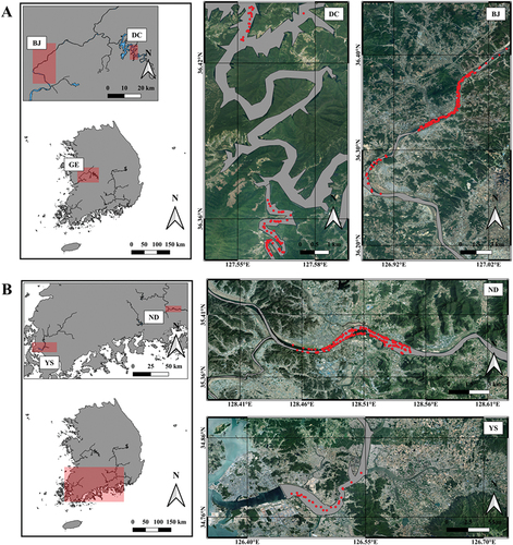
This study selected the Geum (GE), Nakdong (ND), and Yeongsan (YS) rivers – the major rivers of South Korea – as study sites. These rivers are major water supply sources and the water from these rivers is utilized in agricultural, industrial, and domestic water processes in widespread areas (Kim et al. 2017; An et al. 2019). The geographical information of the study area is presented in Table 1. The GE River is located in mid-western South Korea Figure 1(a). The length of main river is 398 km, and its water surface area is 9,915 km². The Daecheong (DC) reservoir and Baekje (BJ) weir have been studied as critical cyanobacterial bloom regions in the GE River. In the DC reservoir (36.35°–36.52°N, 127.48°–127.60°E), the watershed area and storage volume are 4,134 km² and 1,490 × 10⁶ m³, respectively. It has a water surface of 72.8 km², a length of 86 km, and an average water depth of 20 m. The water resource is supplied to Daejeon metropolitan city by the water intake stations, including Chudong intake tower (Xin-Chao et al. 2015). The BJ weir (36.24° – 36.42°N, 126.88° – 127.04°E) region is located downstream of the DC and has a watershed area of 9,912 km² and a stream length of 23 km (Pyo et al. 2019). The BJ movable weir mainly provides the agricultural water and electric supply (Kim, Lee, and Kwang-Guk 2019). The ND River is located in southeast Korea and is the longest river in South Korea Figure 1(b). The water surface area of the ND is 23,817 km², with a length of 525 km (Park and Seok Lee 2002). The monitoring sites in this river were focused on the Changnyeong Haman weir section (36.37°36.40°N, 128.45° – 128.54°E) that supplies the domestic, agricultural, and industrial water resources to Busan metropolitan, Gimhae, and Yangsan cities (Kim et al. 2018). The YS River is located in southwestern South Korea Figure 1(b). The drainage area and discharge volume of the YS are 3,371 km² and 1.5 × 10⁸ m³, respectively. The monitoring area is the Yeongsan dike (34.76° – 34.82°N, 126.45° – 126.55°E), which is located in the YS River estuary, and it supplies the agricultural and industrial water resources. In addition, the discharge from the YS River affects to the coastal ecosystems as a huge impact. The crucial cyanobacterial bloom outbreaks occurred in the study area because of abundant nutrient loading and a long water retention time (Shim, Yong Yoon, and Hyung Lee 2015; Kim, Lee, and Kwang-Guk 2019; Gwak and Kim 2016; Cho and Cho 2017).

Table 1. Geographical information of the Geum (GE), Nakdong (ND), and Yeongsan (YS) rivers, which are the major rivers in South Korea

Main river	Sampling site	Length	Latitude	Longitude	Watershed area	Number of samples(Sampling)	Monitoring period
GE	Daecheong (DC) reservoir	86 km	N 36.35° – 36.52°	E 127.48° – 127.60°	4,134	118 (13)	2016,2018–2020
	Baekje (BJ) weir	23 km	N 36.24° – 36.42°	E 126.88° – 127.04°	9,912	182 (12)	2016, 2018, 2020
ND	Changnyeong Haman weir	525 km	N 36.37° – 36.40°	E 128.45° – 128.54°	23,817	210 (19)	2017–2018
YS	YS dike	136 km	N 34.76° – 34.82°	E 126.45° – 126.55°	3,371	24 (3)	2018

Figure 1. Study area and monitoring sites of the Geum (GE), Nakdong (ND), and Yeongsan (YS) rivers. In the GE River, there are two different monitoring areas: the Daecheong reservoir (DC) and Baekje weir (BJ). Each field monitoring and sampling site is indicated by a red-colored marker.

2.2 Data acquisition

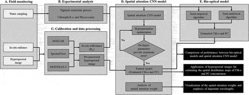
The overall research scheme was divided into five sections Figure 2: (A) data acquisition from water sample field monitoring, field reflectance measurements, and airborne monitoring for hyperspectral images; (B) experimental analysis for extracting Chl-a and PC pigments; (C) hyperspectral image correction preprocessing (radiometric, atmospheric, and geometric correction) via a conversion from raw to reflectance data; (D) construction and training of the spatial attention CNN model; and (E) building bio-optical models, which include semi-empirical and semi-analytical algorithms.

Figure 2. Flowchart for estimating the chlorophyll-a (Chl-a) and phycocyanin (PC) concentrations using the spatial attention convolutional neural network (CNN) model and bio-optical models. (a) indicates the acquisition of the water samples, field reflectance data, and hyperspectral images via field monitoring. (b) and (c) show the experimental analysis of pigments and the processing procedure of reflectance data, respectively. (d) and (e) denote the spatial attention CNN model and bio-optical models, respectively.

2.2.1 Field monitoring and water sampling with experimental analysis

A FieldSpec HandHeld 2 spectroradiometer (ASD Inc., USA) was used to measure the irradiance and radiance from sky and water surface with a viewing angle of 45° from 9 am to 11 am. A range of wavelengths from 350 to 800 nm was selected to consider the data noise of the measurement equipment. Reflectance data were calculated using the method introduced by Mobley (1999), as given below:

(1) $R_{rs}=\frac{L_w-0.025\times L_{sky}}{E_d}$(1)

where the R_rs represents the remote sensing reflectance data [sr⁻¹], L_w is the radiance from the water [W∙m⁻²∙sr⁻¹∙nm⁻¹], L_sky is the radiance from the sky [W∙m⁻²∙sr⁻¹∙nm⁻¹], 0.025 is the reflectance factor (calculated using the wind speed, solar zenith angle, and viewing angle), and E_d is the downwelling irradiance from the sun [W∙m⁻²∙nm⁻¹]. The water samples were collected in two sterilized bottles of different sizes to analyze Chl-a and PC concentrations. In the Chl-a extraction process, 250 mL samples were filtered using glass microfiber filters of 0.7 μm pore size (Whatman Inc., USA). The filters were soaked in an acetone and methanol (9:1) solution for 24 h based on solvent extraction (APHA, American Water Works Association, Water Pollution Control Federation, and Water Environment Federation 1912). The PC water samples were concentrated using a 125 mL plankton net and were homogenized using an ultrasonicator (Sonictopia Inc., South Korea). Then, 20 mL of the homogenized samples were extracted and centrifuged at 4000 rpm for 15 min. Next, the liquid was removed, and the remaining solid sample was mixed with 5 mL of phosphate buffer solution (Sigma-Aldrich, USA). Furthermore, PC extraction was performed using the freezing and thawing method (Bennett and Bogorad 1973). After extracting Chl-a and PC, the absorption spectra from 350 nm to 800 nm were measured using a Cary-5000 UV-Vis-Nir (Ultraviolet-visible-near-infrared) spectrophotometer (Agilent Inc., USA). The absorption spectra data were used to estimate the concentrations of Chl-a and PC, following the method reported by Pyo et al. (2016).

2.2.2 Drone- and air-borne hyperspectral image

Nano-Hyperspec (Headwall Photonics Inc., USA) and AISA Eagle (SPECIM Inc., Oulu, Finland) hyperspectral imaging sensors obtained the optical signal data, and field monitoring was conducted in the DC reservoir and BJ weir, respectively. The drone used was a MATRICE M600 Pro hexacopter (DJI Inc., Shenzhen, China), and an aircraft with the AISA Eagle sensor was operated by ASIA Aero Survey Co., Ltd. The measurement of the hyperspectral image was performed when the wind speed was less 6.0 m/s in order to stabilize the aircraft operation. The drone and aircraft were operated at a flight height of 150 m and 3,000 m, respectively. The drone-borne hyperspectral imaging sensor measured a spectral range of 350–800 nm with a spatial resolution of 20 cm pixel⁻¹ and a spectral resolution of 2.2 nm. The airborne hyperspectral images had a wavelength range of 400 to 970 nm with a spatial resolution of 2 m pixel⁻¹ and a spectral resolution of 4.2 nm. The drone operating could utilize to obtain the reflectance data in the relatively small area such as branches of main river. On the other hand, the air-borne hyperspectral images were suitable to measure the wide area. The calibration and data processing procedures of the drone-borne hyperspectral imagery were implemented using SpectralView (Headwall Photonics Inc., US) based on Kwon et al. (2020). Meanwhile, the airborne hyperspectral images were subjected to image processing using MODTRAN 6 software (Pyo et al. 2018). To minimize the signal noise of the calibrated images, a Savitzky-Golay filter was utilized with the MATLAB (MathWorks Inc., USA) image-processing toolbox (Chen et al. 2004). The Savitzky-Golay filter was a second-order polynomial with the frame lengths of 5. The deep learning model utilized the pretreated hyperspectral images to visualize the distribution maps of algal pigments. The model swept the image as one pixel by one pixel to estimate the concentrations of Chl-a and PC at each pixel. The estimated output data were reconstructed with the same shape as the input hyperspectral images.

2.3 Bio-optical algorithm approach

Semi-empirical and semi-analytical algorithms were adopted to estimate the pigment concentration using apparent optical properties (AOPs) and inherent optical properties (IOPs) (Mishra, Ogashawara, and Abraham Gitelson 2017; Mishra, Schaeffer, and Keith 2014).

2.3.1 Semi-empirical algorithms

The representative semi-empirical algorithm utilized was the band ratio algorithm, which uses two or three bands. This study utilized two- and three-band ratio algorithms to estimate the Chl-a and PC concentrations, respectively. The two band ratio algorithms are given below (Moses et al. 2009; Mishra 2012):

(2) ${\left[\mathrm{C}\mathrm{h}\mathrm{l}-a\right]}_{2B}\left(mg/m^3\right)\propto \frac{R_{rs}\left(708\right)}{R_{rs}\left(665\right)}$(2)

(3) ${\left[\mathrm{P}\mathrm{C}\right]}_{2B}\hspace{0.17em}\left(mg/m^3\right)\propto \frac{R_{rs}\left(708\right)}{R_{rs}\left(600\right)}$(3)

where, [Chl-a]_2B is the concentration of Chl-a calculated by the two band ratio algorithm, [PC]_2B is the PC concentration calculated by the two band ratio algorithm, and R_rs(600), R_rs(665), and R_rs(708) are the remote sensing reflectance [sr⁻¹] at 600 nm, 665 nm, and 708 nm, respectively.

The three-band ratio algorithms are as follows (Hunter et al. 2008; Moses et al. 2009):

(4) ${\left[\mathrm{C}\mathrm{h}\mathrm{l}-a\right]}_{3B}\hspace{0.17em}\left(mg/m^3\right)\propto \left(R_{rs}{\left(665\right)}^{-1}-R_{rs}{\left(708\right)}^{-1}\right)\times R_{rs}\left(753\right),$(4)

(5) ${\left[\mathrm{P}\mathrm{C}\right]}_{3B}\hspace{0.17em}\left(mg/m^3\right)\propto \left(R_{rs}{\left(630\right)}^{-1}-R_{rs}{\left(660\right)}^{-1}\right)\times R_{rs}\left(750\right)$(5)

where, [Chl-a]_3B is the concentration of Chl-a calculated by the three band ratio algorithm, [PC]_3B is the PC concentration calculated by the three band ratio algorithm, R_rs(630), R_rs(660), R_rs(750), and R_rs(753) are the remote sensing reflectance [sr⁻¹] at 630 nm, 660 nm, 750 nm, and 753 nm, respectively.

To optimize the band ratio algorithms for each water body, optimal bands were selected by comparing the accuracy with the observed pigment concentration. The bands were empirically tuned to ensure best performance of the optical band ratio algorithm using MATLAB. The equations of the optimized two- and three-band ratio algorithms are as follows:

(6) $\left[\mathrm{C}\mathrm{h}\mathrm{l}-a\right]{\hspace{0.17em}}_{Optim-2B}\propto \frac{R_{rs}\left({\lambda }_1\right)}{R_{rs}\left({\lambda }_2\right)}$(6)

(7) $\left[\mathrm{P}\mathrm{C}\right]{\hspace{0.17em}}_{Optim-2B}\propto \frac{R_{rs}\left({\lambda }_1\right)}{R_{rs}\left({\lambda }_2\right)}$(7)

(8) $\left[\mathrm{C}\mathrm{h}\mathrm{l}-a\right]{\hspace{0.17em}}_{Optim-3B}\propto \left(R_{rs}{\left({\lambda }_1\right)}^{-1}-R_{rs}{\left({\lambda }_2\right)}^{-1}\right)\times R_{rs}\left({\lambda }_3\right)$(8)

(9) $\left[\mathrm{P}\mathrm{C}\right]{\hspace{0.17em}}_{Optim-3B}\propto \left(R_{rs}{\left({\lambda }_1\right)}^{-1}-R_{rs}{\left({\lambda }_2\right)}^{-1}\right)\times R_{rs}\left({\lambda }_3\right)$(9)

where, [Chl-a]_Optim-2B is the concentration of Chl-a calculated by the optimized two-band ratio algorithm, [PC]_Optim-2B is the PC concentration calculated by the optimized two-band ratio algorithm, [Chl-a]_Optim-3B is the concentration of Chl-a calculated by the optimized three-band ratio algorithm, [PC]_Optim-3B is the PC concentration calculated by the optimized three-band ratio algorithm, and λ₁, λ₂, and λ₃ are the optimized wavelengths. Note that the optimized band ratio algorithms adopted different bands for each water body. The optimized band ratio algorithms were utilized to evaluate the performance of a spatial attention CNN model that could be generalized for different water bodies. Three different optimized band ratio algorithms were constructed for each study area, whereas a spatial attention CNN model was trained on the overall datasets of the three study areas.

2.3.2 Semi-analytical algorithms

AOPs (e.g. radiance, irradiance, and remote sensing reflectance) directly measure the optical properties of a medium. Conversely, IOPs (e.g. absorption and backscattering) consider the inherent properties of the water body and are independent of ambient light. Thus, semi-analytical algorithms have been utilized for IOPs, whereas semi-empirical algorithms are used for AOPs. Gons, Rijkeboer, and Ruddick (2005) and Duan, Ronghua, and Chuanmin (2012) presented the following equations to calculate the concentration of Chl-a:

(10) $a_{chla}\left(\lambda \right)=\hspace{0.17em}\frac{R_{rs}\left(709\right)}{R_{rs}\left(\lambda \right)}\times \left[a_w\left(709\right)+b_b\right]-{b_b}^p-a_w\left(\lambda \right),$(10)

(11) $b_b=\frac{1.61\times R_{rs}\left(778\right)}{0.082-0.6\times R_{rs}\left(778\right)}$(11)

(12) ${\left[\mathrm{C}\mathrm{h}\mathrm{l}-a\right]}_{Gons}\hspace{0.17em}\left(mg/m^3\right)=\frac{a_{chla}\left(665\right)}{a_{chla}^{\ast }\left(665\right)},$(12)

where p is 1.062 [-], $a_{chla}\left(\lambda \right)$ is the absorption coefficient of Chl-a at a specific wavelength, $a_w$ is the absorption coefficient dominated by water, $b_b$ is the backscattering coefficient, and $a_{chla}^{\ast }\left(665\right)$ is the specific absorption coefficient of Chl-a at 665 nm, which is defined as 0.0161 m²/mg. Note that in the Eq. (10(10) $a_{chla}\left(\lambda \right)=\hspace{0.17em}\frac{R_{rs}\left(709\right)}{R_{rs}\left(\lambda \right)}\times \left[a_w\left(709\right)+b_b\right]-{b_b}^p-a_w\left(\lambda \right),$(10) ), $a_w\left(709\right)$ and $a_w\left(665\right)$ are 0.70 m⁻¹ and 0.40 m⁻¹, respectively.

Meanwhile, Simis, Peters, and Gons (2005) proposed a semi-analytical algorithm for estimating the PC concentration as follows:

(13) $a_{chla}\left(665\right)=\left[\frac{R_{rs}\left(709\right)}{R_{rs}\left(665\right)}\times \left(a_w\left(709\right)+b_b\right)\text{break}-b_b-a_w\left(665\right)\right]\times {\gamma }^{-1}$(13)

(14) $a_{pc}\left(620\right)=\left[\frac{R_{rs}\left(709\right)}{R_{rs}\left(620\right)}\times \left(a_w\left(709\right)+b_b\right)\text{break}-b_b-a_w\left(620\right)\right]\times {\delta }^{-1}-\left[\epsilon \times a_{chla}\left(665\right)\right]$(14)

(15) ${\left[\mathrm{P}\mathrm{C}\right]}_{Simis}\hspace{0.17em}\left(mg/m^3\right)=\frac{a_{pc}\left(620\right)}{a_{pc}^{\ast }\left(620\right)}$(15)

where δ, γ, ε, $a_w\left(620\right)$, and $a_{pc}^{\ast }\left(620\right)$ are 0.84 [-], 0.68 [-], 0.24 [-], 0.281 m⁻¹, and 0.007 m²/mg, respectively.

2.4 Data-driven model approach

2.4.1 Input and output composition

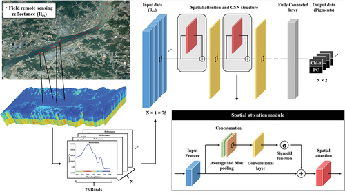
The input dataset was selected as the measured field reflectance data in the wavelength range of 450 to 800 nm to minimize data noise. However, the drone-borne and airborne hyperspectral images had different wavelength intervals and ranges, as they had 90 and 86 bands, respectively. Thus, we related the wavelength bands between the drone-borne and airborne images with 75 bands. The concentrations of Chl-a and PC were normalized using minmax normalization and were then used as output datasets. The total sizes of the input and output datasets were N × 1 × 75 and N × 2, respectively, where N is the number of samples. The datasets were randomly separated into training datasets (70%) and validation datasets (30%).

2.4.2 CNN

In this study, a CNN was applied to derive the features of the remote sensing reflectance data in order to estimate the concentrations of Chl-a and PC. The convolutional layer extracts various features of the data using numerous convolution kernels (also called filters) (LeCun et al. 1989). The kernels obtain the feature data according to the weight and biases, and then move along the input data. The size of the feature data is the same as the size of the input data using padding and stride (Dumoulin and Visin 2016). In this study, a stride of 1 and a padding of (k-1)/2, where k is the kernel size, which has an odd number, was used. The feature data of the convolutional layer are connected by a batch normalization layer for regularization, which can prevent overfitting (Luo et al. 2018). The batch normalization layer implements the normalization of the convolution feature data and is applied to reduce the internal covariate shift (Ioffe and Szegedy 2015). The pooling layer has the advantage of decreasing the size of the feature data and the number of parameters (Aloysius and Geetha 2017). In addition, the speed of the model training was significantly improved by the pooling layer. Moreover, the general pooling methods are max pooling and average pooling (Gholamalinezhad and Khosravi 2020), in which the max pooling method leaves and highlights the maximum values in the pooling regions, and the average pooling method calculates and maintains average values in the pooling regions. The dropout layer is utilized to prevent overfitting by deactivating random nodes of the feature data or FC layer (Srivastava et al. 2014). The deactivation nodes lead to the selection of various combinations of feature data and train the features of nonlinearity (Choe and Shim 2019).

In this study, the 1D CNN model employed three convolutional layers, three batch normalization layers, and a max-pooling layer. The pooling layer and dropout layers were located in front of the two FC layers. Before starting the model training process, a random search was conducted for hyperparameter optimization (Bergstra and Bengio 2012). Through this optimization process, the 1D CNN model determined the number of epochs, learning rate, mini-batch size, kernel size of the convolutional layer, kernel size of the max pooling layer, number of nodes in the FC layer, and type of activation function. The results of the hyperparameter optimization are summarized in Table 2.

Table 2. Descriptions of hyperparameters for the spatial attention convolutional neural network (CNN) model. The values were selected among the ranges of each hyperparameters by the optimization

Hyper-parameter	Equation	Range [Min, Max]	Value
Number of epochs (Nepoch)	50 n + 400	[0, 8]	650
Learning rate (lr)	10^−n	[3, 5]	4
Mini-batch size	2 ^n	[4, 6]	4
Kernel size of the convolutional layer	2 n + 1	[1, 9]	17
Kernel size of the pooling layer	2 n + 1	[1, 9]	17
Number of node in the fully connected (FC) layer	2 ^n	[3, 11]	7
Type of activation function	n	[ReLU, ELU, LeakyReLU, CELU, tanh]	LeakyReLU

2.4.3 Spatial attention network

The CNN model has difficulty accessing the weights of the output of each input variable because it is a black-box model (Koh and Liang 2017). Therefore, CNN models can be implemented using explainable techniques, such as class activation maps (Zhou et al. 2016) or attention networks (Wang et al. 2017). Woo et al. (2018) introduced a convolutional block attention module (CBAM) consisting of a channel attention module and a spatial attention module to explore the model training results using 2-dimensional imagery. The channel attention and spatial attention modules focused on analyzing the channel and spatial relationships, respectively. In this study, the input data covered a 1D structure without channels, allowing the 1D CNN model to be combined with the spatial attention module of the CBAM. The spatial attention module provided informative sections of the input data. First, the average and max pooling methods were applied to the input data to obtain two different results. These results were concatenated to emphasize important features. Then, the convolution layer and sigmoid function were applied to the concatenated result. In the convolutional layer, the kernel size was set to seven. The formulation of the spatial attention module was calculated using

(16) $M_s\left(F\right)=\sigma \left(C^7\left(\left[AugPool\left(F\right);MaxPool\left(F\right)\right]\right)\right)$(16)

where $M_s$ is the spatial attention module, F is the feature data, σ is the sigmoid function, $C^7$ is a convolution layer with a kernel size of 7, AvgPool is the average pooling method, and MaxPool is the max pooling method. The result of the spatial attention module was multiplied with the feature data of the CNN model and added to the residual data Figure 3.

Figure 3. The spatial attention convolutional neural network (CNN) model for estimating the concentrations of chlorophyll-a (Chl-a) and phycocyanin (PC). The input data is the field remote sensing reflectance (R_rs). The dimensions of the input and output data are N × 1 × 75 and N × 2, respectively, where N is the number of field monitoring samples.

2.4.4 Training and validation step

The spatial attention CNN model uses the hyperparameters selected during hyperparameter optimization via numerous model training processes. The model was trained to minimize the loss value, which was calculated as the mean squared error (MSE) between the observed and estimated data, which can be expressed as follows:

(17) $MSE=\frac{1}{n}\sum _{i=1}^n{\left(y_{e,i}-y_{o,i}\right)}^2$(17)

where n is the size of the samples, $y_{e,i}$ is the estimated value [mg/m³] of the spatial attention CNN model, and $y_{o,i}$ is the observed value [mg/m³].

The trained CNN model was evaluated using the correlation coefficient (R) and root mean squared error (RMSE), as follows:

(18) $R=\frac{\sum _{i=1}^n\left(y_{e,i}-{\bar{y}}_{e,i}\right)\left(y_{o,i}-{\bar{y}}_{o,i}\right)}{\sqrt{\sum _{i=1}^n{\left(y_{e,i}-{\bar{y}}_{e,i}\right)}^2}\sqrt{\sum _{i=1}^n{\left(y_{o,i}-{\bar{y}}_{o,i}\right)}^2}},$(18)

(19) $RMSE=\hspace{0.17em}\sqrt{\frac{\sum _{i=1}^n{\left(y_{e,i}-y_{o,i}\right)}^2,}{n}}$(19)

where ${\bar{y}}_{e,i}$ is the average value of the model outputs [mg/m³], and ${\bar{y}}_{o,i}$ is the average value of the observations [mg/m³]. A Taylor diagram was applied to examine the performance of the overall bio-optical algorithms and the spatial attention CNN model (Taylor 2001).

3. Results and discussion

3.1 Observation analysis of cyanobacteria

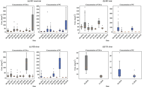
The observed pigment information of cyanobacteria in the different study sites is shown in Figure 4. Overall, the concentration of pigments in the GE River was higher than those in the ND and YS rivers. In the GE River, the highest concentrations of Chl-a and PC were 355.56 mg/m³ and 537.34 mg/m³, respectively. The standard deviations of the GE River were relatively higher than those of the other rivers. Shin, Kang, and Hwang (2016) reported that Chl-a concentrations above 100 mg/m³ have a high probability of health damage caused by cyanobacteria outbreaks in South Korea.

Figure 4. Temporal variation at the (a) Daecheong (DC) reservoir, (b) Baekje (BJ) weir, (c) Nakdong (ND) River, and (d) Yeongsan (YS) River. The concentrations of chlorophyll-a (Chl-a) and phycocyanin (PC) are indicated by gray- and blue-colored boxes, respectively.

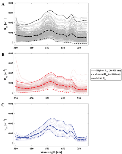
The field R_rs spectra for each study area are shown in Figure 5. The troughs of the R_rs spectra near 620 nm and 670 nm may be due to substantial absorption of water constituents, such as algal pigments. The 670 nm (near 665 nm) wavelength was utilized for the two-band ratio algorithm in Equation 2(2) ${\left[\mathrm{C}\mathrm{h}\mathrm{l}-a\right]}_{2B}\left(mg/m^3\right)\propto \frac{R_{rs}\left(708\right)}{R_{rs}\left(665\right)}$(2) . In addition, 620 nm was adopted to calculate the absorption coefficient of water constituents in Equations 14(14) $a_{pc}\left(620\right)=\left[\frac{R_{rs}\left(709\right)}{R_{rs}\left(620\right)}\times \left(a_w\left(709\right)+b_b\right)\text{break}-b_b-a_w\left(620\right)\right]\times {\delta }^{-1}-\left[\epsilon \times a_{chla}\left(665\right)\right]$(14) and 15(15) ${\left[\mathrm{P}\mathrm{C}\right]}_{Simis}\hspace{0.17em}\left(mg/m^3\right)=\frac{a_{pc}\left(620\right)}{a_{pc}^{\ast }\left(620\right)}$(15) . Meanwhile, relatively high peaks were observed at 560 nm, 650 nm, and 700 nm, indicating low absorption of the pigments. The reflectance at 700 nm is related to extreme algal blooms as the red and NIR regions denote enhanced backscattering effect of algae (Gons 1999). Specifically, at 560 nm, the average reflectance values of the GE and YS rivers were higher than those of ND. The R_rs values of the GE River showed a wide range from 0.003 sr⁻¹ to 0.029 sr⁻¹, whereas the YS samples had relatively high R_rs values above 0.013 sr⁻¹. In contrast, the R_rs values in the ND River were restricted within a narrow range of 0.002 sr⁻¹ to 0.020 sr⁻¹. This may be due to different conditions of water constituents, such as different concentrations of cyanobacterial blooms and suspended sediments (Aurin et al. 2010; Chang et al. 2006). Therefore, ND River had the lowest changes in the R_rs values, even though the differences between the maximum and minimum pigment concentrations were relatively higher in ND River than those in YS River. The water constituents showed variations in the field reflectance data for the different study areas.

Figure 5. Remote sensing reflectance (R_rs) spectra from 350 nm to 800 nm in the (a) Geum (GE), (b) Nakdong (ND), and (c) Yeongsan (YS) rivers. The sample amounts in the GE, ND, and YS rivers are 300, 210 and 24, respectively. The dash-dot and dashed lines represent the highest and lowest R_rs values at 600 nm. The solid line with square markers denotes the mean R_rs values calculated using the total R_rs.

3.2 Performance of bio-optical algorithms

In this study, bio-optical algorithms were used to estimate the pigment concentrations of water samples. As shown in Figure 6(a-b), [Chl-a]_3B had the highest performance in GE and ND rivers (0.84 and 0.82, respectively). Meanwhile, in the YS River, the R values of the band-ratio algorithms showed a low performance of below 0.39. Similarly, the semi-analytical algorithm results were in good agreement with the observed pigments in the GE and ND rivers and revealed low R values (< 0.40) in the YS River Figure 6(c). According to the PC concentration results, [PC]_2B showed high performance with R values reaching 0.77 and 0.67 in the GE and ND rivers, respectively Figure 7(a-b). However, in YS River, the R value of [PC]_3B was 0.64, which is higher than that found by the other band ratio algorithms. The semi-analytical algorithm, [PC]_Simis, exhibited similar performance with the semi-empirical algorithm, revealing R values of 0.84 and 0.67 for the GE and ND rivers Figure 7(c), respectively, and an R value of −0.18 for the YS River. Overall, most of the pigment concentrations estimated using bio-optical algorithms were in good agreement with the observed concentrations in the GE and ND rivers. Conversely, the results for the YS River had relatively low performance because the number of samples was insufficient, as compared with the GE and ND rivers (Oyedare and Jerry Park 2019). This is because water bodies have distinct optical properties based on the different water components (Mobley 1995). Previous studies have utilized various bio-optical algorithms that use optimized bands to enhance the accuracy of Chl-a and PC concentrations in different study sites (Duan et al. 2010; Hunter et al. 2010; Mishra and Mishra 2012; Schalles and Yacobi 2000).

Figure 6. Correlation plots between the observed and estimated chlorophyll-a (Chl-a) concentrations of each study area (Geum (GE), Nakdong (ND), and Yeongsan (YS) rivers) using (a-b) semi-empirical, (c) semi-analytical, (d-e) optimized band ratio algorithms, and (f) the spatial attention convolutional neural network (CNN) model.

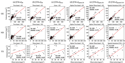
Figure 7. Correlation plots between the observed and estimated phycocyanin (PC) concentrations of each study area (Geum (GE), Nakdong (ND), and Yeongsan (YS) rivers) using (a-b) semi-empirical, (c) semi-analytical, (d-e) optimized band ratio algorithms, and the (f) spatial attention convolutional neural network (CNN) model.

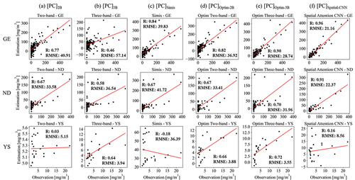
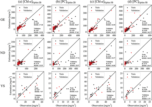
On the basis of R values, specific bands were selected in the present study to show the best algorithm performance for each study area (Table 3). The selected wavelengths of the optimized band ratio algorithms were different from those of the previous algorithms because of the distinct optical properties of different water components in each water body. In particular, the optimized two-band ratio algorithm for PC adopted the disparate wavelengths of 740 nm and 792 nm in the YS River. In contrast, the conventional two-band ratio algorithm utilizes 600 nm and 708 nm to estimate PC concentration (Mishra 2012). The optimized band ratio algorithms obtained Chl-a with an R value above 0.83, which was remarkably higher than that of the semi-empirical and semi-analytical algorithms Figure 6(d-e). Moreover, the optimized three-band ratio algorithm of Chl-a showed an R value above 0.85, and an RMSE value below 16.49 mg/m³. As shown in Figures 7(d-e), the performances of the optimized band ratio algorithms for PC were remarkably higher than those of the other algorithms. Specifically, the R values of [PC]_optim-3B in the GE, ND, and YS rivers were over 0.90, 0.70, and 0.72, respectively. Additionally, the RMSE was below 40.90 mg/m³ for the overall study area. The performances of the overall bio-optical algorithms for each study site are shown in Figures 6 and 7. To identify the training and validation performances of the optimized band ratio algorithms, the scatter plots and model performance were obtained Figure 8. The R values of [Chl-a]_Optim-2B and [PC]_Optim-2B were above 0.78 and 0.69, respectively. In case of the optimized three band ratio algorithms for estimating the validation datasets, the R values of Chl-a and PC were above 0.75 and 0.75, respectively. The overall performances of the optimized band ratio algorithms in the GE River were relatively higher than those in the other two rivers. In general, the optimized three-band ratio algorithms of Chl-a and PC exhibited considerably higher performance than the other algorithms. Thus, band selection optimization is necessary to obtain the best performance of the method used to estimate cyanobacteria in different water bodies. Furthermore, the complex optical properties of inland water led to the construction of various bio-optical algorithms that use optimized bands owing to the different bio-optical characterizations of the water bodies (Morel et al. 2007; Moore et al. 2014; Stambler 2005). Even though the optimized band ratio algorithms showed remarkable performance, it is difficult to construct a generalized model for the three different study areas considered in the present study.

Table 3. Band information for optimizing the band ratio algorithms of each study area (Geum (GE), Nakdong (ND), and Yeongsan (YS) rivers)

Algorithm	Pigment	Target area	λ1 (nm)	λ2 (nm)	λ3 (nm)	Equation
Two-band ratio algorithm	chlorophyll-a (Chl-a)	GE	722	683	-	$\left[\mathrm{C}\mathrm{h}\mathrm{l}-a\right]{\hspace{0.17em}}_{Optim-2B}\propto \frac{R_{rs}\left({\lambda }_1\right)}{R_{rs}\left({\lambda }_2\right)}$
		ND	716	667	-
		YS	651	659	-
	phycocyanin (PC)	GE	723	619	-	$\left[\mathrm{P}\mathrm{C}\right]{\hspace{0.17em}}_{Optim-2B}\propto \frac{R_{rs}\left({\lambda }_1\right)}{R_{rs}\left({\lambda }_2\right)}$
		ND	708	685	-
		YS	792	740	-
Three-band ratio algorithm	Chl-a	GE	702	688	763	$\left[\mathrm{C}\mathrm{h}\mathrm{l}-a\right]{\hspace{0.17em}}_{Optim-3B}\propto \left(R_{rs}{\left({\lambda }_1\right)}^{-1}-R_{rs}{\left({\lambda }_2\right)}^{-1}\right)\times R_{rs}\left({\lambda }_3\right)$
		ND	714	581	723
		YS	662	651	676
	PC	GE	577	569	759	$\left[\mathrm{P}\mathrm{C}\right]{\hspace{0.17em}}_{Optim-3B}\propto \left(R_{rs}{\left({\lambda }_1\right)}^{-1}-R_{rs}{\left({\lambda }_2\right)}^{-1}\right)\times R_{rs}\left({\lambda }_3\right)$
		ND	653	623	698
		YS	708	702	760

Figure 8. Correlation plots between the observed and estimated chlorophyll-a (Chl-a) and phycocyanin (PC) concentrations over the entire study area using the optimized two band ratio algorithms (a-b) and the optimized three band ratio algorithms (c-d). The train and validation datasets are indicated by black and red markers, respectively.

3.3 Estimating the spatial attention CNN model

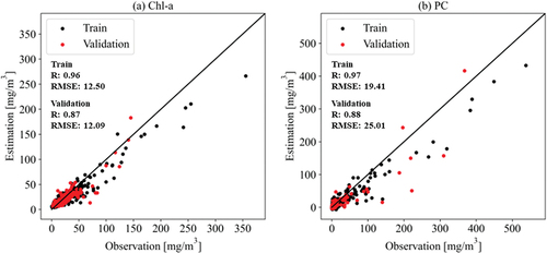
Chl-a and PC concentrations were estimated using a spatial attention CNN model. The correlations for the entire study area are shown in Figure 9. The R and RMSE values of the Chl-a were above 0.87 and below 12.09 mg/m³, respectively. Meanwhile, for the PC, the R value of the validation was 0.88, and the RMSE was 25.01 mg/m³. The estimated pigment concentrations were in good agreement with the observed pigment concentrations for the three study areas. The spatial attention CNN model was generalized by training the overall data without separating the datasets. In addition, the overall performance of the spatial attention CNN model was remarkably higher than those of the bio-optical algorithms.

Figure 9. Correlation plots between the observed and estimated (a) chlorophyll-a (Chl-a) and (b) phycocyanin (PC) concentrations over the entire study area using the spatial attention convolutional neural network (CNN) model. The train and validation datasets are indicated by black and red markers, respectively.

The correlation and model performance of each study area are shown in Figures 6(f) and 7(f). The R values of Chl-a and PC were above 0.91 and the RMSE values were below 18.81 mg/m³ in the GE and ND rivers. Compared with the bio-optical algorithms, the spatial attention CNN model showed the highest accuracy in the GE and ND rivers Figure 10. Thus, the samples in the GE and ND rivers were acceptable for training the various spatiotemporal variations of the pigments using the CNN model and showed good performance. Meanwhile, the [Chl-a]_Spatial-CNN model for the YS River had a similar R value (0.85) as the [Chl-a]_Optim-3B model but had high RMSE value of 10.15 mg/m³ compared to the model (8.27 mg/m³). In addition, the [PC]_Spatial-CNN of the YS River had a significantly low correlation (0.16) with the observed data compared with the optimized band ratio algorithms. The high performance of the spatial attention CNN model in the GE and ND rivers can be attributed to the high number of samples. According to Zhu et al. (2016), the performance of a data-driven model can be improved by increasing the training data, which is known as effectiveness of big data. In contrast, the number of samples in the YS River was only 24, and the different trends observed in the reflectance data might have caused low accuracy when the spatial attention CNN model was used for estimation of pigment concentration. In addition, the field reflectance data in the YS River revealed higher R_rs values than those in the GE and ND rivers Figure 5(c). The irregular reflectance patterns in samples from YS River may have resulted in the poor estimation of the PC concentration as the deep learning model trains the representative features of most datasets (Das, Datta, and Chaudhuri 2018). The performance of spatial attention CNN model may be further improved by obtaining sufficient datasets to train the model for various water bodies.

Figure 10. Performance evaluation of the (a) chlorophyll-a (Chl-a) and (b) phycocyanin (PC) estimation models for each study area using Taylor diagrams. The Taylor diagram indicates the standard deviation [mg/m³], correlation coefficient (R), and root mean squared error (RMSE) [mg/m³].

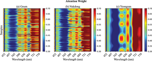
3.4 Sensitivity analysis for identifying representative optical features

The spatial attention module indicated that the important R_rs bands in the CNN model that used quantitative attention weights Figure 11. Overall, similar patterns of attention weight were observed but slight differences were observed in some samples. Specifically, the range of wavelength between 693 nm and 800 nm had considerably higher attention weights than the other bands in the study area. The range between 693 nm and 800 nm are located in the red and near-infrared (NIR) regions. According to Richardson (1996) and Gons (1999), the red and NIR reflectance were high when a critical algal bloom occurred due to the dominant backscattering effect of algae. In particular, 708 nm was utilized for the band ratio algorithms to estimate both Chl-a and PC concentrations. Han and Rundquist (1997) reported that the band ratio algorithm using 705 nm showed a remarkable correlation with the concentration of Chl-a. Gitelson (1992) employed a two-band ratio of 700 nm to consider the combined absorption of algal pigments. The wavelengths near 600 nm and 650 nm also indicated relatively higher attention weights, according to the band ratio algorithms that used these wavelengths to calculate the PC and Chl-a, respectively. Mishra, Mishra, and Schluchter (2009) reported that the band obtained near 600 nm showed the maximum absorption related to the PC concentration without the effect of Chl-a. Similarly, the absorption of Chl-a and PC increased in the band near 650 nm (Schalles and Yacobi 2000). Bio-optical algorithms, including semi-empirical and semi-analytical algorithms, examine reflectance using these band regions (Mishra, Ogashawara, and Abraham Gitelson 2017). Thus, the spatial attention CNN model utilized the bands at 600 nm, 650 nm, and the NIR region as the important factors in the training process for estimating the concentrations of Chl-a and PC. Although the model performance in the YS River was relatively insufficient, the features of the visualized data had a similar pattern to that of the entire study area. However, the CNN model prioritized the features of the GE and ND rivers because the datasets in the GE and ND rivers were significantly higher than those of the YS River. Although the pigments in the YS River were relatively low in concentration, the spatial attention CNN model still prioritized the red and NIR regions, which are related to a high concentration of algal blooms. In addition, the red and NIR regions can be utilized to estimate the high concentrations of Chl-a and PC, such as in the samples of the GE and ND rivers. The relatively low model performance might be the result of the different features of pigment variations in the YS River.

Figure 11. Visualization of the attention weights in each study area. Significant wavelengths are indicated in red (relatively high weight value), and insignificant wavelengths are denoted by blue (relatively low weight value).

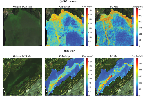
The spatial attention CNN model swept the images as one pixel by one pixel and used it as input data. After the estimation of pigment concentrations, the output data were reconstructed to the same size as the initial hyperspectral images. The spatial distribution maps of algal pigments were visualized using the spatial attention CNN model and the drone-borne and airborne hyperspectral images in the GE River Figure 12. As shown in Figure 12(a), the hyperspectral image was obtained by drone-borne remote sensing, and the distribution map showed the salt and pepper noises. These noises might be caused by the low signal of the hyperspectral sensor and the application method of the distribution maps. The spatial attention CNN model estimated that the lakeside regions had remarkably high pigment concentrations, reaching above 300 mg/m³. Moreover, as these regions have relatively slow water velocity, it may aggravate cyanobacteria outbreaks (Susana et al. 2013). The model results showed relatively low concentrations of Chl-a and PC at the center of the reservoir. In contrast, as shown in Figure 12(b), abundant algal blooms line in the middle of the river. As the water discharge near the weir spillway increases the water velocity, algal blooms gather and flow into the spillway (Park et al. 2017). These results suggest that the spatial attention CNN model can be used to estimate the spatial distributions of cyanobacteria blooms over a wide target area using hyperspectral imagery. The utilization of the drone-borne and airborne hyperspectral images could improve the generalization ability of the spatial attention CNN model. Furthermore, the spatial attention CNN model has a possibility to expand to extensive areas, including different water bodies, by using the satellite remote sensing imagery.

Figure 12. Distribution maps of chlorophyll-a (Chl-a) and phycocyanin (PC) concentrations by (a) drone-borne hyperspectral image in Daecheong (DC) reservoir and (b) airborne hyperspectral image in Baekje (BJ) weir. The left column images are the original RGB images.

4. Conclusions

This study aimed to estimate the concentrations of harmful algal pigments in various water bodies using a spatial attention CNN model and to subsequently compare its performance with that of conventional bio-optical algorithms. Furthermore, the spatial attention module was also applied to calculate the attention weights and identify the importance of the reflectance bands in the model training process. As the results, the bio-optical algorithms showed different performances according to the utilized bands and target area. In the GE and ND rivers, the conventional bio-optical algorithms had R values above 0.82 and 0.67 for Chl-a and PC, respectively. The selection of optimized bands and the performance of the bio-optical algorithms were influenced by the specific optical characteristics of individual water bodies. The spatial attention CNN model showed good performance with above 0.91 of R value in the GE and ND rivers. However, the results in the YS River showed a poor correlation as 0.16 of R value for PC because of the different reflectance input features and a lack of training data. The spatial attention module identified and visualized the importance of input wavelengths for training the CNN model. Specifically, the spatial attention CNN model utilized the NIR region, which represents the backscattering effect of water and the absorption of pigments. In addition, the bands at 600 nm and 650 nm were used to consider the absorption of Chl-a and PC.

This study demonstrated the capability of generalization of spatial attention CNN model to estimate cyanobacteria outbreak in various water bodies. In future research, the uncertainties of the deep learning model can be further improved by acquiring sufficient datasets. The model can be applied to all streams by utilizing Sentinel-2 or Landsat 8 satellite imagery to overcome the limitations of drone-borne and airborne remote sensing methods. By utilization of multispectral satellite data, the spatial attention CNN model could estimate the distribution maps of Chl-a and PC on entire streams in South Korea and could be expanded to other countries that had the similar water conditions.

Acknowledgements

This research was supported by the Water Environmental and Infrastructure Research Program (NIER-2021-01-01-058) funded by the National Institute of Environmental Research; the ICT R&D program of MSIT/IITP (2018-0-00219, Space-time complex artificial intelligence blue-green algae prediction technology based on direct-readable water quality complex sensor and hyperspectral image); and the Korea Environment Industry & Technology Institute (KEITI) through the “Aquatic Ecosystem Conservation Research Program” funded by the Korea Ministry of Environment (MOE) [No. 2020003050001].

Disclosure statement

No potential conflict of interest was reported by the author(s).

Data availability statement

The data that support the findings of this study are available from the corresponding author, J.C. Pyo, upon reasonable request.

References

- Ahishali, M., S. Kiranyaz, T. Ince, and M. Gabbouj. 2021. “Classification of Polarimetric SAR Images Using Compact Convolutional Neural Networks.” GIScience & Remote Sensing 58 (1): 28–47. doi:10.1080/15481603.2020.1853948.
- Ali, K. A., J. Ortiz, N. Bonini, M. Shuman, and C. Sydow. 2016. “Application of Aqua MODIS Sensor Data for Estimating Chlorophyll a in the Turbid Case 2 Waters of Lake Erie Using Bio-optical Models.” GIScience & Remote Sensing 53 (4): 483–505. doi:10.1080/15481603.2016.1177248.
- Aloysius, N., and M. Geetha. 2017. “A Review on Deep Convolutional Neural Networks.” Paper presented at the 2017 International Conference on Communication and Signal Processing (ICCSP) (pp. 0588-0592). doi:10.1109/ICCSP.2017.8286426.
- Ammenberg, P., P. Flink, T. Lindell, D. Pierson, and N. Strombeck. 2002. “Bio-optical Modelling Combined with Remote Sensing to Assess Water Quality.” International Journal of Remote Sensing 23 (8): 1621–1638. doi:10.1080/01431160110071860.
- An, S.-U., J.-S. Mok, S.-H. Kim, J.-H. Choi, and J.-H. Hyun. 2019. “A Large Artificial Dyke Greatly Alters Partitioning of Sulfate and Iron Reduction and Resultant Phosphorus Dynamics in Sediments of the Yeongsan River Estuary, Yellow Sea.” Science of the Total Environment 665: 752–761. doi:10.1016/j.scitotenv.2019.02.058.
- APHA, American Water Works Association, Water Pollution Control Federation, and Water Environment Federation. 1912. Standard Methods for the Examination of Water and Wastewater. Vol. 2. Washington, DC, USA: American Public Health Association.
- Aurin, D. A., H. M. Dierssen, M. S. Twardowski, and C. S. Roesler. 2010. “Optical Complexity in Long Island Sound and Implications for Coastal Ocean Color Remote Sensing.” Journal of Geophysical Research: Oceans 115 (C7). doi:10.1029/2009JC005837.
- Bennett, A., and L. Bogorad. 1973. “Complementary Chromatic Adaptation in a Filamentous Blue-green Alga.” Journal of Cell Biology 58 (2): 419–435. doi:10.1083/jcb.58.2.419.
- Bergstra, J., and Y. Bengio. 2012. “Random Search for Hyper-parameter Optimization.” Journal of Machine Learning Research 13 (2): 281–305.
- Bosse, K. R., M. J. Sayers, R. A. Shuchman, G. L. Fahnenstiel, S. A. Ruberg, D. L. Fanslow, D. G. Stuart, T. H. Johengen, and A. M. Burtner. 2019. “Spatial-temporal Variability of in Situ Cyanobacteria Vertical Structure in Western Lake Erie: Implications for Remote Sensing Observations.” Journal of Great Lakes Research 45 (3): 480–489. doi:10.1016/j.jglr.2019.02.003.
- Carmichael, W. W., and G. L. Boyer. 2016. “Health Impacts from Cyanobacteria Harmful Algae Blooms: Implications for the North American Great Lakes.” Harmful Algae 54: 194–212. doi:10.1016/j.hal.2016.02.002.
- Chang, G. C., A. H. Barnard, S. McLean, P. J. Egli, J. R. V. Z. Casey Moore, T. D. Dickey, and A. Hanson. 2006. “In Situ Optical Variability and Relationships in the Santa Barbara Channel: Implications for Remote Sensing.” Applied Optics 45 (15): 3593–3604. doi:10.1364/ao.45.003593.
- Chen, J., P. Jönsson, M. Tamura, G. Zhihui, B. Matsushita, and L. Eklundh. 2004. “A Simple Method for Reconstructing A High-quality NDVI Time-series Data Set Based on the Savitzky–Golay Filter.” Remote Sensing of Environment 91 (3–4): 332–344. doi:10.1016/j.rse.2004.03.014.
- Chen, L., H. Zhang, J. Xiao, L. Nie, J. Shao, W. Liu, and T.-S. Chua. 2017. “Sca-cnn: Spatial and Channel-wise Attention in Convolutional Networks for Image Captioning.” Paper presented at the Proceedings of the IEEE conference on computer vision and pattern recognition (CVPR), pp. 5659-5667.
- Cho, H.-C., and Y.-G. Cho. 2017. “Long-term Variation and Flux of Organic Carbon in the Human-disturbed Yeongsan River, Korea.” The Sea 22 (4): 187–198. doi:10.7850/jkso.2017.22.4.187.
- Choe, J., and H. Shim. 2019. “Attention-based Dropout Layer for Weakly Supervised Object Localization.” Paper presented at the Proceedings of the IEEE/CVF Conference on Computer Vision and Pattern Recognition (CVPR), pp. 2219-2228.
- D’Sa, E. J. 2014. “Assessment of Chlorophyll Variability along the Louisiana Coast Using Multi-satellite Data.” GIScience & Remote Sensing 51 (2): 139–157. doi:10.1080/15481603.2014.895578.
- Das, S., S. Datta, and B. B. Chaudhuri. 2018. “Handling Data Irregularities in Classification: Foundations, Trends, and Future Challenges.” Pattern Recognition 81: 674–693. doi:10.1016/j.patcog.2018.03.008.
- Dev, P. J., A. Sukenik, D. R. Mishra, and I. Ostrovsky. 2022. “Cyanobacterial Pigment Concentrations in Inland Waters: Novel Semi-analytical Algorithms for Multi-and Hyperspectral Remote Sensing Data.” Science of the Total Environment 805: 150423. doi:10.1016/j.scitotenv.2021.150423.
- Duan, H., M. Ronghua, and H. Chuanmin. 2012. “Evaluation of Remote Sensing Algorithms for Cyanobacterial Pigment Retrievals during Spring Bloom Formation in Several Lakes of East China.” Remote Sensing of Environment 126: 126–135. doi:10.1016/j.rse.2012.08.011.
- Duan, H., M. Ronghua, X. Jingping, Y. Zhang, and B. Zhang. 2010. “Comparison of Different Semi-empirical Algorithms to Estimate Chlorophyll-a Concentration in Inland Lake Water.” Environmental Monitoring and Assessment 170 (1): 231–244. doi:10.1007/s10661-009-1228-7.
- Dumoulin, V., and F. Visin. 2016. “A Guide to Convolution Arithmetic for Deep Learning.” arXiv preprint arXiv:1603.07285.
- Fangling, P., C. Ding, Z. Chao, Y. Yue, and X. Xin. 2019. “Water-quality Classification of Inland Lakes Using Landsat8 Images by Convolutional Neural Networks.” Remote Sensing 11 (14): 1674. doi:10.3390/rs11141674.
- Fauvel, M., Y. Tarabalka, J. Atli Benediktsson, J. Chanussot, and J. C. Tilton. 2012. “Advances in Spectral-spatial Classification of Hyperspectral Images.” Proceedings of the IEEE 101 (3): 652–675. doi:10.1109/JPROC.2012.2197589.
- Gatys, L. A., A. S. Ecker, and M. Bethge. 2016. “Image Style Transfer Using Convolutional Neural Networks.” Paper presented at the Proceedings of the IEEE conference on computer vision and pattern recognition (CVPR), pp. 2414-2423.
- Gerten, D., and R. Adrian. 2002. “Effects of Climate Warming, North Atlantic Oscillation, and El Nino-Southern Oscillation on Thermal Conditions and Plankton Dynamics in Northern Hemispheric Lakes.” TheScientificWorldJOURNAL 2: 586–606. doi:10.1100/tsw.2002.141.
- Gholamalinezhad, H., and H. Khosravi. 2020. “Pooling Methods in Deep Neural Networks, a Review.” arXiv preprint arXiv:2009.07485.
- Gitelson, A. 1992. “The Peak near 700 Nm on Radiance Spectra of Algae and Water: Relationships of Its Magnitude and Position with Chlorophyll Concentration.” International Journal of Remote Sensing 13 (17): 3367–3373. doi:10.1080/01431169208904125.
- Gobler, C. J. 2020. “Climate Change and Harmful Algal Blooms: Insights and Perspective.” Harmful Algae 91: 101731. doi:10.1016/j.hal.2019.101731.
- Gons, H. J. 1999. “Optical Teledetection of Chlorophyll a in Turbid Inland Waters.” Environmental Science & Technology 33 (7): 1127–1132. doi:10.1021/es9809657.
- Gons, H. J., M. Rijkeboer, and K. G. Ruddick. 2005. “Effect of a Waveband Shift on Chlorophyll Retrieval from MERIS Imagery of Inland and Coastal Waters.” Journal of Plankton Research 27 (1): 125–127. doi:10.1093/plankt/fbh151.
- Gwak, B.-R., and I.-K. Kim. 2016. “Characterization of Water Quality in Changnyeong-Haman Weir Section Using Statistical Analyses.” Journal of Korean Society of Environmental Engineers 38 (2): 71–78. doi:10.4491/KSEE.2016.38.2.71.
- Han, L., and D. C. Rundquist. 1997. “Comparison of NIR/RED Ratio and First Derivative of Reflectance in Estimating Algal-chlorophyll Concentration: A Case Study in A Turbid Reservoir.” Remote Sensing of Environment 62 (3): 253–261. doi:10.1016/S0034-4257(97)00106-5.
- Hunter, P. D., A. N. Tyler, L. Carvalho, G. A. Codd, and S. C. Maberly. 2010. “Hyperspectral Remote Sensing of Cyanobacterial Pigments as Indicators for Cell Populations and Toxins in Eutrophic Lakes.” Remote Sensing of Environment 114 (11): 2705–2718. doi:10.1016/j.rse.2010.06.006.
- Hunter, P. D., A. N. Tyler, M. Présing, A. W. Kovács, and T. Preston. 2008. “Spectral Discrimination of Phytoplankton Colour Groups: The Effect of Suspended Particulate Matter and Sensor Spectral Resolution.” Remote Sensing of Environment 112 (4): 1527–1544. doi:10.1016/j.rse.2007.08.003.
- Ioffe, S., and C. Szegedy. 2015. “Batch Normalization: Accelerating Deep Network Training by Reducing Internal Covariate Shift.” Paper presented at the International conference on machine learning (PMLR), pp. 448-456.
- Jiang, P., X. Liu, J. Zhang, T. Shu Harn, K. Y.-H. Gin, Y. Van-Fan, J. Jaromír Klemes, and C. A. Shoemaker. 2021. “Cyanobacterial Risk Prevention under Global Warming Using an Extended Bayesian Network.” Journal of Cleaner Production 127729. doi:10.1016/j.jclepro.2021.127729.
- Jin, Q., H. Lyu, L. Shi, S. Miao, W. Zhiming, L. Yunmei, and Q. Wang. 2017. “Developing a Two-step Method for Retrieving Cyanobacteria Abundance from Inland Eutrophic Lakes Using MERIS Data.” Ecological Indicators 81: 543–554. doi:10.1016/j.ecolind.2017.06.027.
- Jupp, D. L. B., J. T. O. Kirk, and G. P. Harris. 1994. “Detection, Identification and Mapping of Cyanobacteria—using Remote Sensing to Measure the Optical Quality of Turbid Inland Waters.” Marine & Freshwater Research 45 (5): 801–828. doi:10.1071/MF9940801.
- Kelvin, X., B. Jimmy, R. Kiros, K. Cho, A. Courville, R. Salakhudinov, R. Zemel, and Y. Bengio. 2015. “Show, Attend and Tell: Neural Image Caption Generation with Visual Attention.” Paper presented at the International conference on machine learning (PMLR), pp. 2048-2057.
- Kim, Y. H., S. Hong, Y. Sik Song, H. Lee, H.-C. Kim, J. Ryu, J. Park, B.-O. Kwon, C.-H. Lee, and J. Seong Khim. 2017. “Seasonal Variability of Estuarine Dynamics Due to Freshwater Discharge and Its Influence on Biological Productivity in Yeongsan River Estuary, Korea.” Chemosphere 181: 390–399. doi:10.1016/j.chemosphere.2017.04.085.
- Kim, Y.-J., S.-J. Lee, and A. Kwang-Guk. 2019. “Characteristics of Chemical Water Quality and the Empirical Model Analysis before and after the Construction of Baekje Weir.” Korean Journal of Environmental Biology 37 (1): 48–59. doi:10.11626/KJEB.2019.37.1.048.
- Kim, T.-W., H.-S. Yang, B.-W. Park, and J.-S. Yoon. 2018. “Study on Water Level and Salinity Characteristics of Nakdong River Estuary Area by Discharge Variations at Changnyeong-Haman Weir (1).” Journal of Ocean Engineering and Technology 32 (5): 361–366. doi:10.26748/KSOE.2018.6.32.5.361.
- Koh, P. W., and P. Liang. 2017. “Understanding Black-box Predictions via Influence Functions.” Paper presented at the International Conference on Machine Learning (PMLR), pp. 1885-1894.
- Kwon, Y. S., J. Pyo, Y.-H. Kwon, H. Duan, K. Hwa Cho, and Y. Park. 2020. “Drone-based Hyperspectral Remote Sensing of Cyanobacteria Using Vertical Cumulative Pigment Concentration in a Deep Reservoir.” Remote Sensing of Environment 236: 111517. doi:10.1016/j.rse.2019.111517.
- LeCun, Y., B. Boser, J. S. Denker, D. Henderson, R. E. Howard, W. Hubbard, and L. D. Jackel. 1989. “Backpropagation Applied to Handwritten Zip Code Recognition.” Neural Computation 1 (4): 541–551. doi:10.1162/neco.1989.1.4.541.
- Lee, J., M. Kim, I. Jungho, H. Han, and D. Han. 2021. “Pre-trained Feature Aggregated Deep Learning-based Monitoring of Overshooting Tops Using Multi-spectral Channels of GeoKompsat-2A Advanced Meteorological Imagery.” GIScience & Remote Sensing 58 (7): 1052–1071.
- Liu, T., A. Abd-Elrahman, J. Morton, and V. L. Wilhelm. 2018. “Comparing Fully Convolutional Networks, Random Forest, Support Vector Machine, and Patch-based Deep Convolutional Neural Networks for Object-based Wetland Mapping Using Images from Small Unmanned Aircraft System.” GIScience & Remote Sensing 55 (2): 243–264. doi:10.1080/15481603.2018.1426091.
- Liu, H., H. Baoyin, Y. Zhou, X. Yang, X. Zhang, F. Xiao, Q. Feng, S. Liang, X. Zhou, and F. Congju. 2021. “Eutrophication Monitoring of Lakes in Wuhan Based on Sentinel-2 Data.” GIScience & Remote Sensing 58 (5): 776–798. doi:10.1080/15481603.2021.1940738.
- Luo, P., X. Wang, W. Shao, and Z. Peng. 2018. “Towards Understanding Regularization in Batch Normalization.” arXiv preprint arXiv:1809.00846.
- Manning, S. R., and D. R. Nobles. 2017. “Impact of Global Warming on Water Toxicity: Cyanotoxins.” Current Opinion in Food Science 18: 14–20. doi:10.1016/j.cofs.2017.09.013.
- Matthews, M. W., S. Bernard, and K. Winter. 2010. “Remote Sensing of Cyanobacteria-dominant Algal Blooms and Water Quality Parameters in Zeekoevlei, a Small Hypertrophic Lake, Using MERIS.” Remote Sensing of Environment 114 (9): 2070–2087. doi:10.1016/j.rse.2010.04.013.
- Mei, X., E. Pan, M. Yong, X. Dai, J. Huang, F. Fan, Q. Du, H. Zheng, and M. Jiayi. 2019. “Spectral-spatial Attention Networks for Hyperspectral Image Classification.” Remote Sensing 11 (8): 963. doi:10.3390/rs11080963.
- Mishra, S. 2012. “Remote sensing of cyanobacteria in turbid productive waters.“ Mississippi State University, 2012.
- Mishra, S., and D. R. Mishra. 2012. “Normalized Difference Chlorophyll Index: A Novel Model for Remote Estimation of Chlorophyll-A Concentration in Turbid Productive Waters.” Remote Sensing of Environment 117: 394–406. doi:10.1016/j.rse.2011.10.016.
- Mishra, S., D. R. Mishra, and W. M. Schluchter. 2009. “A Novel Algorithm for Predicting Phycocyanin Concentrations in Cyanobacteria: A Proximal Hyperspectral Remote Sensing Approach.” Remote Sensing 1 (4): 758–775. doi:10.3390/rs1040758.
- Mishra, D. R., I. Ogashawara, and A. Abraham Gitelson. 2017. Bio-optical Modeling and Remote Sensing of Inland Waters. Amsterdam, Netherlands: Elsevier.
- Mishra, D. R., B. A. Schaeffer, and D. Keith. 2014. “Performance Evaluation of Normalized Difference Chlorophyll Index in Northern Gulf of Mexico Estuaries Using the Hyperspectral Imager for the Coastal Ocean.” GIScience & Remote Sensing 51 (2): 175–198. doi:10.1080/15481603.2014.895581.
- Mobley, C. D. 1995. “The Optical Properties of Water.” Handbook of Optics 1: 43.3-.56.
- Mobley, C. D. 1999. “Estimation of the Remote-sensing Reflectance from Above-surface Measurements.” Applied Optics 38 (36): 7442–7455. doi:10.1364/AO.38.007442.
- Moore, T. S., M. D. Dowell, S. Bradt, and A. Ruiz Verdu. 2014. “An Optical Water Type Framework for Selecting and Blending Retrievals from Bio-optical Algorithms in Lakes and Coastal Waters.” Remote Sensing of Environment 143: 97–111. doi:10.1016/j.rse.2013.11.021.
- Moore, S. K., N. J. Mantua, B. M. Hickey, and V. L. Trainer. 2009. “Recent Trends in Paralytic Shellfish Toxins in Puget Sound, Relationships to Climate, and Capacity for Prediction of Toxic Events.” Harmful Algae 8 (3): 463–477. doi:10.1016/j.hal.2008.10.003.
- Morel, A., H. Claustre, D. Antoine, and B. Gentili. 2007. “Natural Variability of Bio-optical Properties in case 1 Waters: Attenuation and Reflectance within the Visible and near-UV Spectral Domains, as Observed in South Pacific and Mediterranean Waters.” Biogeosciences 4 (5): 913–925. doi:10.5194/bg-4-913-2007.
- Moses, W. J., A. A. Gitelson, S. Berdnikov, and V. Povazhnyy. 2009. “Satellite Estimation of Chlorophyll-$ a $ Concentration Using the Red and NIR Bands of MERIS—the Azov Sea Case Study.” IEEE Geoscience and Remote Sensing Letters 6 (4): 845–849. doi:10.1109/LGRS.2009.2026657.
- Oyedare, T., and J.-M. Jerry Park. 2019. “Estimating the Required Training Dataset Size for Transmitter Classification Using Deep Learning.” Paper presented at the 2019 IEEE International Symposium on Dynamic Spectrum Access Networks (DySPAN), 11–14 November 2019, Newark, NJ, USA.
- Park, Y., J. Pyo, Y. Sung Kwon, Y. Cha, H. Lee, T. Kang, and K. Hwa Cho. 2017. “Evaluating Physico-chemical Influences on Cyanobacterial Blooms Using Hyperspectral Images in Inland Water, Korea.” Water Research 126: 319–328. doi:10.1016/j.watres.2017.09.026.
- Park, S. S., and Y. Seok Lee. 2002. “A Water Quality Modeling Study of the Nakdong River, Korea.” Ecological Modelling 152 (1): 65–75. doi:10.1016/S0304-3800(01)00489-6.
- Paul, A., S. Bhattacharya, D. Dutta, J. Raj Sharma, and V. Kumar Dadhwal. 2015. “Band Selection in Hyperspectral Imagery Using Spatial Cluster Mean and Genetic Algorithms.” GIScience & Remote Sensing 52 (6): 643–659. doi:10.1080/15481603.2015.1075180.
- Pei, W., S. Yao, S. Dong, J. F. Knight, X. Chong, and Y. Chen. 2015. “Using Field Spectral Measurements to Estimate Chlorophyll-a in Waterlogged Areas of Huainan, China.” GIScience & Remote Sensing 52 (6): 660–679. doi:10.1080/15481603.2015.1082173.
- Peterson, K. T., V. Sagan, and J. J. Sloan. 2020. “Deep Learning-based Water Quality Estimation and Anomaly Detection Using Landsat-8/Sentinel-2 Virtual Constellation and Cloud Computing.” GIScience & Remote Sensing 57 (4): 510–525. doi:10.1080/15481603.2020.1738061.
- Pyo, J., H. Duan, S. Baek, M. Sung Kim, T. Jeon, Y. Sung Kwon, H. Lee, and K. Hwa Cho. 2019. “A Convolutional Neural Network Regression for Quantifying Cyanobacteria Using Hyperspectral Imagery.” Remote Sensing of Environment 233: 111350. doi:10.1016/j.rse.2019.111350.
- Pyo, J. C., M. Ligaray, Y. Sung Kwon, M.-H. Ahn, K. Kim, H. Lee, T. Kang, S. Been Cho, Y. Park, and K. Hwa Cho. 2018. “High-spatial Resolution Monitoring of Phycocyanin and Chlorophyll-a Using Airborne Hyperspectral Imagery.” Remote Sensing 10 (8): 1180. doi:10.3390/rs10081180.
- Pyo, J., H. SeongHyeon, Y. A. Pachepsky, H. Lee, H. Rim, G. Nam, M. S. Kim, I. Jungho, and K. Hwa Cho. 2016. “Chlorophyll-a Concentration Estimation Using Three Difference Bio-optical Algorithms, Including a Correction for the Low-concentration Range: The Case of the Yiam Reservoir, Korea.” Remote Sensing Letters 7 (5): 407–416. doi:10.1080/2150704X.2016.1142680.
- Ralston, D. K., B. A. Keafer, M. L. Brosnahan, and D. M. Anderson. 2014. “Temperature Dependence of an Estuarine Harmful Algal Bloom: Resolving Interannual Variability in Bloom Dynamics Using a Degree‐day Approach.” Limnology and Oceanography 59 (4): 1112–1126. doi:10.4319/lo.2014.59.4.1112.
- Richardson, L. L. 1996. “Remote Sensing of Algal Bloom Dynamics.” BioScience 46 (7): 492–501. doi:10.2307/1312927.
- Riese, F. M., and S. Keller. 2019. “Soil Texture Classification with 1D Convolutional Neural Networks Based on Hyperspectral Data.” arXiv preprint arXiv:1901.04846. doi:10.5194/isprs-annals-IV-2-W5-615-2019.
- Rostam, N. A. P., N. Hashimah Ahamed Hassain Malim, R. Abdullah, A. Latif Ahmad, B. Seng Ooi, and D. Juinn Chieh Chan. 2021. “A Complete Proposed Framework for Coastal Water Quality Monitoring System with Algae Predictive Model.” IEEE Access 9: 108249–108265. doi:10.1109/ACCESS.2021.3102044.
- Schalles, J. F., and Y. Z. Yacobi. 2000. “Remote Detection and Seasonal Patterns of Phycocyanin, Carotenoid and Chlorophyll Pigments in Eutrophic Waters.” Ergebnisse Der Limnologie 55: 153–168.
- Shi, K., Y. Zhang, B. Qin, and B. Zhou. 2019. “Remote Sensing of Cyanobacterial Blooms in Inland Waters: Present Knowledge and Future Challenges.” Science Bulletin 64 (20): 1540–1556.
- Shim, M. J., J. Yong Yoon, and S. Hyung Lee. 2015. “Water Quality Properties of Tributaries of Daechung Lake, Korea.” Korean Journal of Ecology and Environment 48 (1): 12–25. doi:10.11614/KSL.2015.48.1.012.
- Shin, J.-K., B.-G. Kang, and S.-J. Hwang. 2016. “Water-blooms (Green-tide) Dynamics of Algae Alert System and Rainfall-hydrological Effects in Daecheong Reservoir, Korea.” Korean Journal of Ecology and Environment 49 (3): 153–175. doi:10.11614/KSL.2016.49.3.153.
- Simis, S. G. H., S. W. M. Peters, and H. J. Gons. 2005. “Remote Sensing of the Cyanobacterial Pigment Phycocyanin in Turbid Inland Water.” Limnology and Oceanography 50 (1): 237–245. doi:10.4319/lo.2005.50.1.0237.
- Sothe, C., C. M. De Almeida, M. B. Schimalski, L. E. C. La Rosa, J. D. B. Castro, R. Q. Feitosa, M. Dalponte, C. L. Lima, V. Liesenberg, and G. T. Miyoshi. 2020. “Comparative Performance of Convolutional Neural Network, Weighted and Conventional Support Vector Machine and Random Forest for Classifying Tree Species Using Hyperspectral and Photogrammetric Data.” GIScience & Remote Sensing 57 (3): 369–394. doi:10.1080/15481603.2020.1712102.
- Srivastava, N., G. Hinton, A. Krizhevsky, I. Sutskever, and R. Salakhutdinov. 2014. “Dropout: A Simple Way to Prevent Neural Networks from Overfitting.” The Journal of Machine Learning Research 15 (1): 1929–1958.
- Stambler, N. 2005. “Bio-optical Properties of the Northern Red Sea and the Gulf of Eilat (Aqaba) during Winter 1999.” Journal of Sea Research 54 (3): 186–203. doi:10.1016/j.seares.2005.04.006.
- Stumpf, R. P., T. W. Davis, T. T. Wynne, J. L. Graham, K. A. Loftin, T. H. Johengen, D. Gossiaux, D. Palladino, and A. Burtner. 2016. “Challenges for Mapping Cyanotoxin Patterns from Remote Sensing of Cyanobacteria.” Harmful Algae 54: 160–173. doi:10.1016/j.hal.2016.01.005.
- Susana, R., J. Soria, F. Fernandez, Y. Ouahid, and Á. N. G. E. L. Barón‐solá. 2013. “Water Residence Time and the Dynamics of Toxic Cyanobacteria.” Freshwater Biology 58 (3): 513–522. doi:10.1111/j.1365-2427.2012.02734.x.
- Taylor, K. E. 2001. “Summarizing Multiple Aspects of Model Performance in a Single Diagram.” Journal of Geophysical Research: Atmospheres 106 (D7): 7183–7192. doi:10.1029/2000JD900719.
- Thamaga, K. H., and T. Dube. 2019. ““Understanding Seasonal Dynamics of Invasive Water Hyacinth (Eichhornia Crassipes) in the Greater Letaba River System Using Sentinel-2 Satellite Data.” GIScience & Remote Sensing 56 (8): 1355–1377. doi:10.1080/15481603.2019.1646988.
- Tomlinson, M. C., R. P. Stumpf, T. T. Wynne, D. Dupuy, R. Burks, J. Hendrickson, and R. S. Fulton III. 2016. “Relating Chlorophyll from Cyanobacteria-dominated Inland Waters to a MERIS Bloom Index.” Remote Sensing Letters 7 (2): 141–149. doi:10.1080/2150704X.2015.1117155.
- Wang, F., M. Jiang, C. Qian, S. Yang, L. Cheng, H. Zhang, X. Wang, and X. Tang. 2017. “Residual Attention Network for Image Classification.” Paper presented at the Proceedings of the IEEE conference on computer vision and pattern recognition (CVPR), pp. 3156-3164.
- Wang, X., H. Song, Y. Wang, and N. Chen. 2021. “Research on the Biology and Ecology of the Harmful Algal Bloom Species Phaeocystis Globosa in China: Progresses in the Last 20 Years.” Harmful algae:102057.
- Woo, S., J. Park, J.-Y. Lee, and I. So Kweon. 2018. “Cbam: Convolutional Block Attention Module.” Paper presented at the Proceedings of the European conference on computer vision (ECCV), pp. 3-19.
- Woźniak, M., K. M. Bradtke, M. Darecki, and A. Krężel. 2016. “Empirical Model for Phycocyanin Concentration Estimation as an Indicator of Cyanobacterial Bloom in the Optically Complex Coastal Waters of the Baltic Sea.” Remote Sensing 8 (3): 212. doi:10.3390/rs8030212.
- Xin-Chao, M., B.-S. Lim, S.-U. Heo, and M. Kwak. 2015. “Variation of Water Quality around the Chudong Intake Tower in Daechung Reservoir.” Journal of Korean Society on Water Environment 31 (6): 637–643. doi:10.15681/KSWE.2015.31.6.637.
- Yadav, D. P., A. S. Jalal, D. Garlapati, K. Hossain, A. Goyal, and G. Pant. 2020. “Deep Learning-based ResNeXt Model in Phycological Studies for Future.” Algal Research 50: 102018. doi:10.1016/j.algal.2020.102018.
- Zhou, B., A. Khosla, A. Lapedriza, A. Oliva, and A. Torralba. 2016. “Learning Deep Features for Discriminative Localization.” Paper presented at the Proceedings of the IEEE conference on computer vision and pattern recognition (CVPR), pp. 2921-2929.
- Zhu, X., C. Vondrick, C. C. Fowlkes, and D. Ramanan. 2016. “Do We Need More Training Data?” International Journal of Computer Vision 119 (1): 76–92. doi:10.1007/s11263-015-0812-2.