Upscaling aboveground biomass of larch (Larix olgensis Henry) plantations from field to satellite measurements: a comparison of individual tree-based and area-based approaches

ABSTRACT

Currently, aboveground biomass (AGB) estimation primarily relies on an area-based approach (ABA), particularly at a large scale. With the advancement of individual tree detection techniques and the availability of multi-platform remotely sensed data, the individual tree-based approach (ITA) provides the potential of accurate and nondestructive fine AGB mapping. However, the performances of the two approaches on upscaling AGB from individual tree to stand level have not been thoroughly investigated. This study conducted the nondestructive AGB estimation using both ITA and ABA and compared the AGB estimates and their spatial uncertainties from an individual tree- to stand-level based on multi-platform LiDAR and Landsat 8 OLI imagery, taking Larix olgensis that is one of the most notable afforestation tree species in northeastern China as an example. Results showed that the point cloud segmentation (PCS) outperformed CHM-based individual tree crown delineation algorithms and obtained the highest accuracy of individual tree AGB estimate (R² = 0.97, RMSE = 28.58 kg, rRMSE = 21.13%) for the dense larch plantations (about 1265 trees/ha). The plot-level AGB estimate aggregated by all detected trees and its uncertainty based on Monte Carlo simulation were 158.16 and 3.64 Mg·ha⁻¹, respectively. The average pixel-level AGB of larch plantations in Maorshan Forest Farm estimated by ITA and ABA were similar (129.66 v.s 144.38 Mg·ha⁻¹). ITA outperformed ABA in terms of pixel-level AGB accuracy and spatial uncertainty of pixel-level and stand-level AGB estimates. The overestimation of low AGB values, typical in ABA, was effectively eliminated by the ITA. The upscaling frameworks proposed in this study for AGB estimation and spatial uncertainty quantification based on ITA and ABA could be extended to other plantations or uncomplex forests. This study contributes to the accurate quantification of AGB and understanding of the uncertainties in the carbon stock of forest ecosystems at multi-scales.

KEYWORDS:

• LiDAR
• AGB
• spatial uncertainty
• ITA
• ABA

1. Introduction

In the context of global warming caused by CO₂ and other greenhouse gases, the international community started the reduce deforestation and forest degradation (REDD+) plan (Angelsen 2009). REDD+ aims to reduce the destruction in developing countries and increase forest carbon sinks through forest protection and sustainable forest management to mitigate climate change (Ji et al. 2017). The emission reduction projects described in the REDD+ require robust methods to quantify large-scale forest carbon sinks. Due to forest biomass and carbon stocks equivalence, the forest’s carbon stocks mainly focus on forest biomass estimation. Forest biomass includes aboveground biomass (AGB), belowground biomass, coarse woody debris, litter, and soil organic matter (Satoo and Madgwick 2012). AGB, which can be subdivided into trunk, branch, and foliage biomass, accounts for the most significant forest biomass and could be direct measured and indirect estimated (West 2009). Accurately quantifying forest AGB is crucial for understanding global change-related issues such as the carbon cycle and climate change (Gleason and Im 2011; Zhang et al. 2022). The most accurate method to estimate forest biomass is harvest measurements. However, the traditional field survey data is time-consuming and labor-intensive, and it is impossible to cover large-areas (Lu et al. 2016). Due to the advantages of nondestructive, continuous, and spatially explicit remote sensing data, large-area AGB is mainly achieved by applying remotely sensed data, such as optical imagery, light detection and ranging (LiDAR) data, and radio detection and ranging (RADAR) data.

Without the restriction of light conditions, LiDAR data has been widely applied in forest inventory and monitoring since the laser beam can penetrate forests directly and obtain three-dimensional (3-D) canopy information (e.g. Zhen et al. 2015; Zhao et al. 2017; Du et al. 2021; Hao et al. 2022). LiDAR systems can be classified based on different forms of the echo signal (discrete returns or all returns), platforms (Satellite Laser Scanning, Airborne Laser Scanning (ALS), Unmanned Aerial Vehicle Laser Scanning (ULS), Terrestrial Laser Scanning (TLS), or Backpack Laser Scanning (BLS)), and footprint size (small footprint:~1 m, medium footprint: ~10-30 m or large footprint ~50 m)(Lu et al. 2012). LiDAR could be currently the most effective tool to assess forest biomass after the suitable algorithms have been applied (Lee, Kim, and Choi 2013). And, the synergistic utilization of LiDAR and multispectral data is particularly beneficial to estimate various forest parameters (e.g. Du et al. 2021; Manzanera et al. 2016).

In recent years, researchers have utilized small footprint LiDAR data for forest AGB estimation based on either individual tree-based approach (ITA) (e.g. Popescu 2007; Zhao, Popescu, and Nelson 2009; Fu et al. 2018; Qiu et al. 2019) or area-based approach (ABA) (e.g. Li et al. 2014; Su et al. 2016; Cao et al. 2018; Du et al. 2021). The ABA extracts features from remote sensing data at the plot or stand level and establishes a statistical model for estimating the forest AGB of the entire study area (Chen 2013). Features, estimation models, reference data are the most critical factors for ABA. The ABA method has an obvious advantage in the AGB estimation and mapping of large scale (Chen et al. 2016; Su et al. 2016), and have been applied in different forest types, such as boreal forests (Lei et al. 2012), tropical forests (Saatchi et al. 2011; Ometto et al. 2014), and temperate forests (Latifi et al. 2015; Li et al. 2015; Meng et al. 2016).

Since sample plots are the basic units for model fitting and validation for ABA, it is a challenge to obtain enough sample plots. Only a few studies have applied a large number of forest inventory plots for AGB estimation (Næsset and Gobakken 2008; Su et al. 2016). Moreover, it is challenging to investigate biomass uncertainties at different spatial scales due to the lack of detailed information on individual trees (Wang et al. 2009; Xu et al. 2018). In contrast, ITA estimates AGB at an individual tree level and aggregates them into a plot- or stand-level. Thus, the ITA based on individual trees could not only increase the sample size but allow the error propagation of AGB estimation in an up-scaling framework (Xu et al. 2018).

Since ITA estimates forest parameters (e.g. AGB) based on individual trees, an accurate individual tree crown delineation (ITCD) algorithm is significant. Individual tree crown, one of the basic forest parameters, could be applied in various forest-related studies such as biomass and carbon stock estimation (Fang et al. 2016). Over the past two decades, various ITCD algorithms have been developed to improve accuracy, such as maximum local filtering (Ene, Næsset, and Gobakken 2012; Smits et al. 2012), valley following (Leckie et al. 2003), region growing-based methods (Hyyppä et al. 2001; Zhen et al. 2015; Hamraz, Contreras, and Zhang 2017), watershed segmentation (Koch, Heyder, and Weinacker 2006; Jing et al. 2012), region-based hierarchical cross-section analysis (Zhao et al. 2017), hierarchical region-merging algorithm (Hao et al. 2022), and so on. The improvement of classic algorithms or innovative approaches makes it possible to delineate individual trees under more complex forest conditions (e.g. closed hardwood forests, natural secondary forests), especially with the assistance of LiDAR data (Zhen, Quackenbush, and Zhang 2016). Compared to the ABA, ITA makes it easier to understand biomass uncertainties at different spatial scales and estimate plot-level biomass and error propagation in an upscaling framework (Xu et al. 2018).

The main steps of AGB estimation based on the ITA include (1) individual tree crown delineation; (2) estimation of the individual tree parameters (e.g. diameter at breast height (DBH), tree height); (3) individual tree species classification; (4) individual tree AGB estimation using allometric growth equations; (5) aggregation of individual tree-level AGB to plot or stand level. During the procedure, various error sources would influence the AGB estimation and need to be quantified. Standard methods to quantify the error budget included Monte Carlo simulation (Chen, Laurin, and Valentini 2015), Taylor series (Gertner, Cao, and Zhu 1995), polynomial regression (Gertner, Parysow, and Guan 1996), and so on. Some studies have explored the uncertainty caused by different error sources during the AGB estimation procedure (Wang et al. 2009; Cohen et al. 2013; Montesano et al. 2014; Chen, Laurin, and Valentini 2015; Shettles, Hilker, and Temesgen 2016). However, it is complicated to determine how errors are propagated from individual tree level to plot or pixel level due to the diversity of error sources and the limitations of ITCD techniques (Chen, Laurin, and Valentini 2015; Xu et al. 2018). Therefore, how to quantify the various errors in the AGB estimation based on the individual tree method and how the error propagation differs between ITA and ABA, especially for natural secondary forests, are still significant and attractive to the communities of both forestry and remote sensing.

To better understand the spatial distribution and uncertainties of AGB estimations of larch plantations in northeastern China, this study aimed to investigate the nondestructive AGB estimations using both ITA and ABA and conduct the upscaling of the two methods from an individual tree-, plot-, pixel-, then to stand-level using ULS-BLS, ALS, and Landsat 8 OLI imagery data. The specific objectives of this study were to: (1) estimate individual tree parameters (tree height, DBH) using four ITCD methods based on ULS-BLS data; (2) estimate individual tree- and plot-level AGB and explore the spatial uncertainties from an individual tree- to plot-level using Monte Carlo simulation; (3) estimate pixel- and stand-level AGB using ITA and ABA, and explore the spatial uncertainties using Monte Carlo simulation. This study proposed a practical workflow of upscaling the AGB of a typical tree species (i.e. Larix olgensis) in northeast China from field to satellite measurements and comparing the effects of ITA and ABA on the multi-scale AGB estimations. This study would provide a sound foundation for investigating fine AGB mapping at a broader scale and quantifying multi-scale spatial uncertainties of natural secondary forests of northeastern China in the future.

2. Materials and methods

2.1. Study area

The study area is located in Maoershan Experimental Forest Farm, Shangzhi City, Heilongjiang Province, China (Figure 1), which ranges from 127°29′E to 127°44′E and 45°14′N to 45°29′N. It is about 80 km away from Harbin city, the capital of Heilongjiang Province, and belongs to the west slope of Zhangguangcailing in the Changbai Mountains. The total area of the study area is 26,496 ha. The terrain is mountainous, rising from south to north with the highest peak of 805 m and an average elevation of about 300 m.

Figure 1. The location of the study area: (a) The location of Harbin in Heilongjiang Province, P.R. China (China Map Examination No. is GS (2019) 1822); (b) The location of Maoershan Experimental Forest Farm in Shangzhi of Harbin; (c) The location of sample plots in Maoershan. The projection coordinate system for (b) and (c) is WGS 1984 UTM Zone 52 N.

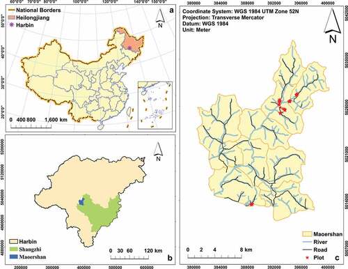
Maoershan belongs to a temperate continental monsoon climate, with an annual average temperature of about 2.4°C and annual precipitation of about 700 mm (Zhao et al. 2022). The vegetation in the Maoershan area belongs to Changbai plant flora due to the location, with the original zonal top-level community of Korean pine broad-leaved forest (Du et al. 2021; Zhang, Yuan, and Zhang 2008). The forests are currently dominated by natural secondary forests and plantations (e.g. Korean pine and larch), with an average forest coverage rate of 95%. The dominant tree species include Pinus koraiensis, Picea koraiensis, Pinus sylvestris var. mongolica, Larix olgensis, Fraxinus mandschurica, Juglans mandshrica, Quercus mongolica, Tilia amurensis, Acer saccharum, Ulmus pumila, Betula platyphylla, Populus davidiana (Liu, Li, and Peng 2017). Larch (Larix olgensis) plantations account for about 62% of all the plantations in Maoershan.

2.2. Data and preprocessing

2.2.1. LiDAR data and preprocessing

Three types of LiDAR data were used in this study, including Unmanned Aerial Vehicle Laser Scanning (ULS) data, Backpack Laser Scanning (BLS) data, and Airborne Laser Scanning (ALS) data. The ULS and BLS data were applied for individual tree AGB estimation, whereas ALS data was applied for area-based AGB estimation. The ULS data with a total area of about 1 km² were acquired in August 2020 using Feima D200 UAV with LiDAR200 system. The BLS data were acquired in 22 sample plots of larch plantations in August and September 2020 using the GreenValley LiBackPack50 system. The central and four corners of each plot were recorded using Global Navigation Satellite System (GNSS) Real-time kinematic positioning (RTK) for georeferencing BLS. The ALS data were acquired in September 2015 using the LiCHy airborne observation system designed by the Chinese Academy of Forestry (CAF) (Hao et al. 2019; Pang et al. 2016). The system was mounted on a fixed-wing aircraft and equipped with a RIEGL LMS-Q680i LiDAR sensor. The essential parameters of the three LiDAR data are described in Table 1.

Table 1. The essential parameters of the three LiDAR data

Parameters	ULS	BLS	ALS
Sensor	Rigel mini VUX-1UAV	VLP16	Rigel LMS-Q680i
Wavelength (nm)	905	903	1550
Laser pulse repetition rate (kHz)	100	300	200
Ranging accuracy (cm)	±1	±3	±2
Scan frequency (Hz)	10 ~ 100	5 ~ 20	10 ~ 200
Echo intensity (bit)	16	16	16
Field of view-horizontal (°)	360	360	60
Field of view-vertical (°)	–	−15°~15°	–
Measuring range (m)	>250	<100	30 ~ 1350

Note: ULS, BLS and ALS are the abbreviation of unmanned aerial vehicle, backpack and airborne laser scanning, respectively.

The preprocessing of ULS data, BLS data, and ALS data included: (1) noise elimination, such as air points, low points, and isolated points. (2) The classification of ground and non-ground points using improved progressive triangular irregular network (TIN) densification approach (Zhao et al. 2016b). (3) The normalization of point clouds. A digital terrain model (DTM) with 0.5 m was generated based on ground points using TIN interpolation (Khosravipour, Skidmore, and Isenburg 2016). The preprocessing of all the LiDAR data was implemented using LiDAR360 V5.0 of GreenValley International.

2.2.2. Landsat 8 OLI imagery and preprocessing

The Landsat 8 OLI imagery (coordinate system: WGS 1984 UTM zone 52 N) with a cloud cover of 0.57% used in this study was acquired on September 24^th, 2019 (downloaded from https://earthexplorer.usgs.gov/). The season of imagery acquisition was consistent with the time that BLS and field survey data were obtained (August and September). This study used seven spectral bands (band 1 to 7) with a pixel size of 30 m. The scene ID of the imagery is LC81170282019267LGN00, which is the L1-TP grade product that has been implemented topographic and geometric correction. The Fast Line-of-sight Atmospheric Analysis of Hypercubes (FLAASH) method was implemented for atmospheric correction. Radiometric and atmospheric correction of Landsat 8 OLI imagery were conducted using ENVI 5.3 software.

2.2.3. Reference data

Since the purpose of this study is to investigate the error propagation from individual-tree level, plot-level to stand-level biomass, the plot size used in this study was designed based on the nominal spatial resolution of Landsat 8 OLI imagery (30 m × 30 m). A total of 22 sample plots of larch plantations that just matched the pixels of Landsat 8 OLI imagery were selected in Maoershan Experimental Forest Farm according to different site conditions and stand ages. The parameters of 2451 trees, including diameter at breast height (DBH, cm), tree height (H, m), and tree location, were obtained in August and September 2020. DBH and tree height were measured using a perimeter ruler and Vertex IV ultrasonic instrument system, respectively, with a starting diameter of 5 cm. Each tree was positioned using an RTK Global Positioning System receiver with a less than 5 cm positional error. The four corners of each plot were positioned as the coordinates of pixels of Landsat 8 OLI imagery in the field using an RTK global positioning system receiver as well in order to avoid geolocation mismatching between field data and remotely sensed data.

The reference of individual tree AGB in this study was calculated using the additive biomass model of larch plantations proposed by Dong (2015), which was the summation of the stem, branches, and foliage biomass of each tree. The additive biomass equations are shown as follows.

(1) $\begin{array}{c}\left\{\begin{array}{c}\begin{array}{c}\mathrm{l}\mathrm{n}{W}_s=-4.5363+1.7008\cdot lnD+1.4804\cdot lnH\\ \mathrm{l}\mathrm{n}{W}_b=-3.3632+2.6728\cdot lnD-0.7052\cdot lnH\end{array}\\ \mathrm{l}\mathrm{n}{W}_f=-2.2879+1.3369\cdot lnD-0.0922\cdot \mathrm{l}\mathrm{n}H\\ ln{W}_a=ln\left(W_s+W_b+W_f\right)\end{array}\right.\end{array}$(1)

Where $W_s$, $W_b$, $W_f$, and $W_a$ represent stem, branches, foliage, and aboveground biomass (kg), respectively; D represents DBH (cm); H represents tree height (m). The descriptive statistics of individual tree parameters of 22 larch plantations plots are listed in Table 2. The plot-level AGB (Mg·ha⁻¹) was an aboveground biomass density which was the sum of AGB of all the individual trees in each plot and then divided by the plot area (0.09 ha).

Table 2. Descriptive statistics for individual tree parameters of all the 22 larch plantations plots, including tree height (H, m), diameter at breast height (DBH, cm) and aboveground biomass (AGB, kg)

Parameters	N	Min	Max	Mean	Median	Standard deviation
H (m)	2451	3.60	27.80	14.52	12.10	5.63
DBH (cm)	2451	6.00	42.50	15.40	12.90	7.61
AGB (kg)	2451	3.58	951.38	113.16	41.28	149.86

2.3 Methods

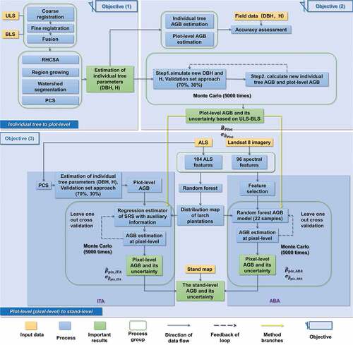
Since the plots were designed to match the pixels of Landsat 8 OLI imagery, the geolocation mismatch between remote sensing and field measurements was avoided to the most extent. The 22 plot-level AGB was a “bridge” between individual tree-level AGB and the pixel-level AGB covering the entire study area. To achieve the nondestructive AGB estimation at the individual-tree level, plot-level, pixel-level, and stand-level, and to analyze and quantify the spatial uncertainty of each level, three modules were designed in this study. Figure 2 shows the flowchart of this study. Module 1 was designed for the first objective of this study, including registration and fusion of the ULS data and BLS data, individual tree crown delineation, and the estimation of individual tree parameters (i.e. DBH and tree height). Module 2 was designed to achieve the second objective, including the individual tree-level and plot-level AGB estimation; and the uncertainty analysis of plot-level AGB using the Monte Carlo simulation. Module 3 was designed for the third objective, including extraction of larch plantations, the pixel-level AGB estimation and its uncertainty using ITA and ABA, the stand-level AGB estimation and its uncertainty.

Figure 2. The flowchart of nondestructive AGB estimation and spatial uncertainty analysis using both ITA and ABA from an individual tree- to stand-level based on multi-platform LiDAR and Landsat 8 OLI imagery. Module 1 was designed for the first objective: data registration and fusion, individual tree crown delineation, and the estimation of individual tree parameters. Module 2 was designed for the second objective: individual tree-level and plot-level AGB estimation and the uncertainty analysis of plot-level AGB using the MC simulation. Module 3 was designed for the third objective: pixel-level AGB estimation and its uncertainty using ITA and ABA, the stand-level AGB estimation and its uncertainty.

2.3.1. Estimation of individual tree parameters

2.3.1.1 Registration and fusion of multi-source data

The ULS and BLS data were registered and fused to generate a ULS-BLS dataset for obtaining a satisfactory accuracy of individual tree crown delineation and parameters estimation. First, the coarse registration was implemented using the four-parameter coordinate transformation model simplified from the Bursa seven-parameter formula (Peng and Deng 2017). Second, BLS data was re-registered to ULS data by the Iterative Closest Points (ICP) method (Arun, Huang, and Blostein 1987; Besl and Mckay 1992). The ICP method minimized the difference between two points clouds and was usually applied to reconstruct a 2-D or 3-D surface from different scans of the same object.

2.3.1.2. Individual tree crown delineation

Based on the ULS-BLS data, four ITCD algorithms, including point cloud segmentation (PCS) (Li et al. 2012), watershed segmentation (WS) (Chen et al. 2006), seeded region growing (SRG) (Mehnert and Jackway 1997), and region hierarchical cross-sectional analysis (RHCSA) (Zhao et al. 2017), were applied to delineate individual trees in this study. For PCS algorithm, we applied density-based spatial clustering of applications with noise (DBSCAN) algorithm (Wu, Cawse-Nicholson, and Aardt 2013) to detect the stem of each tree.

The accuracy assessment of ITCD algorithms was based on 1:1 matched trees, which were defined by the following three-step procedure: (1) to find all the detected trees within a buffer of 3 m of every reference tree; (2) to determine only one detected tree that has the smallest differences of DBH and tree height with the reference tree; (3) to delete the outliers that had the absolute values of external studentized residuals greater than 3. We applied three indices, including recall (r), precision (p), and F-score (Goutte and Gaussier 2005; Sokolova, Japkowicz, and Szpakowicz 2006), to evaluate the performance of ITCD algorithms. The following equations calculated the three indices:

(2) $\begin{array}{c}\begin{array}{c}r=\frac{TP}{\left(TP+FN\right)}\\ \end{array}\end{array}$(2)

(3) $\begin{array}{c}p=\frac{TP}{\left(TP+FP\right)}\end{array}$(3)

(4) $\begin{array}{c}F\mathrm{\_}score=2\times \frac{r\times p}{\left(r+p\right)}\end{array}$(4)

Where TP represented true positive that a tree was correctly detected, that is, 1:1 matched trees; FN represented false negative that a tree is undetected; FP represented false positive that a non-existent tree was detected.

2.3.1.3 The estimation of individual tree parameters

The local maxima within each tree crown delineated from various methods were extracted as tree height. The individual tree parameters (i.e. DBH and tree height) were directly extracted from the PCS algorithm based on the LiDAR point cloud. However, it is not easy to estimate DBH from the three methods (i.e. WS, SRG, RHCSA) that segmented trees based on the CHM. Thus, the non-linear least-squares fitting circle algorithm (Gander 1994) was applied to estimate the DBH of each segmented tree for the three CHM-based methods. The position of the treetop was treated as the tree location.

In this study, the coefficient of determination (R²) of the regression between estimated and measured parameters, root mean square error (RMSE) and relative root mean square error (rRMSE) of estimated parameters were applied to evaluate the accuracy of individual tree parameters estimation (i.e. DBH and height) based on 1:1 matched trees. The equations were shown as follows,

(5) $\begin{array}{c}{R}^2=\frac{{\sum }_{i=1}^n{\left(x_i^{\prime }-\bar{x}\right)}^2}{{\sum }_{i=1}^n{\left(x_i-\bar{x}\right)}^2}\end{array}$(5)

(6) $\begin{array}{c}RMSE=\sqrt{\frac{1}{n}\sum _{i=1}^n{\left(x_i-{x_i}^{\prime }\right)}^2}\end{array}$(6)

(7) $\begin{array}{c}rRMSE=\frac{RMSE}{{\bar{x}}_i}\times 100\mathrm{\%}\end{array}$(7)

where $x_i$ represented the measured tree height or DBH, ${\bar{x}}_i$ represented the average of measured tree height or DBH of an individual tree, ${x_i}^{\prime }$ represented the estimated tree height or DBH.

2.3.2. Plot-level AGB estimation and its uncertainty

The individual tree AGB was calculated using the estimated DBH and tree height based on equation (1)(1) $\begin{array}{c}\left\{\begin{array}{c}\begin{array}{c}\mathrm{l}\mathrm{n}{W}_s=-4.5363+1.7008\cdot lnD+1.4804\cdot lnH\\ \mathrm{l}\mathrm{n}{W}_b=-3.3632+2.6728\cdot lnD-0.7052\cdot lnH\end{array}\\ \mathrm{l}\mathrm{n}{W}_f=-2.2879+1.3369\cdot lnD-0.0922\cdot \mathrm{l}\mathrm{n}H\\ ln{W}_a=ln\left(W_s+W_b+W_f\right)\end{array}\right.\end{array}$(1) . Then, the plot AGB was aggregated by the individual tree AGB in each plot. Since the uncertainty of plot-level AGB estimation could result from various procedures, the error propagation was analyzed by Monte Carlo (MC) simulation, which simulated the occurrence process of a random event repeatedly and was suitable for investigating complicated problems. In MC simulation, a statistical distribution of error source is identified, random samples from each distribution are selected to represent the input parameters, and then the output is obtained according to the input parameters (Raychaudhuri 2008). The MC simulation used in this study was designed to better understand the error propagation from an individual-tree level to a plot-level AGB.

Step 1. To simulate the error of estimated DBH and tree height based on ITCD and obtain a new DBH and tree height. The new residual values ${\epsilon }_d^{\prime }$ and ${\epsilon }_h^{\prime }$ were obtained according to the error distribution of the estimated DBH (d) and tree height (h), respectively. Then, the new DBH and tree height were calculated by Equation (8)(8) $\begin{array}{c}\left\{\begin{array}{c}d{ }^{\mathrm{\prime }}=d+{\epsilon }_d^{\prime }\\ h{ }^{\mathrm{\prime }}=h+{\epsilon }_h^{\prime }\end{array}\right.\end{array}$(8) .

(8) $\begin{array}{c}\left\{\begin{array}{c}d{ }^{\mathrm{\prime }}=d+{\epsilon }_d^{\prime }\\ h{ }^{\mathrm{\prime }}=h+{\epsilon }_h^{\prime }\end{array}\right.\end{array}$(8)

where $d{ }^{\mathrm{\prime }}$ and $h{ }^{\mathrm{\prime }}$ represented the newly generated DBH and tree height, respectively; d and h represented the estimated DBH and tree height of the ITCD algorithm, respectively; ${\epsilon }_d^{\prime }$ and ${\epsilon }_h^{\prime }$ were the new residual values that were randomly generated from the error distribution of the estimated DBH and tree height, respectively. We assumed the residual of DBH and tree height followed a normal distribution with the mean of zero and the variance of the residuals of DBH and tree height, that is,

(9) $\begin{array}{c}{\epsilon }_d^{\prime }\sim \left(0,{{\sigma }_d}^2\right)\end{array}$(9)

(10) $\begin{array}{c}{\epsilon }_h^{\prime }\sim \left(0,{{\sigma }_h}^2\right)\end{array}$(10)

where the ${\sigma }_d$ and ${\sigma }_h$ were the residual standard error of DBH and tree height, respectively.

Step 2. To calculate the new individual tree AGB and plot-level AGB based on the simulated DBH and tree height. The simulated DBH and tree height were applied to obtain a new individual tree AGB using equation (1)(1) $\begin{array}{c}\left\{\begin{array}{c}\begin{array}{c}\mathrm{l}\mathrm{n}{W}_s=-4.5363+1.7008\cdot lnD+1.4804\cdot lnH\\ \mathrm{l}\mathrm{n}{W}_b=-3.3632+2.6728\cdot lnD-0.7052\cdot lnH\end{array}\\ \mathrm{l}\mathrm{n}{W}_f=-2.2879+1.3369\cdot lnD-0.0922\cdot \mathrm{l}\mathrm{n}H\\ ln{W}_a=ln\left(W_s+W_b+W_f\right)\end{array}\right.\end{array}$(1) . Then, the error of estimating individual tree parameters was considered into the new individual tree AGB (${\hat{B}}_{tree}^{\ast }$). The new plot-level AGB (${\hat{B}}_{plot}^{\prime }$) was the accumulated by all the new individual tree AGB, as shown in Equation (11)(11) $\begin{array}{c}{\hat{B}}_{plot}^{\prime }=\frac{1}{S}\left(\sum _{i=1}^N{\hat{B}}_{tree,i}^{\ast }\right)\end{array}$(11) .

(11) $\begin{array}{c}{\hat{B}}_{plot}^{\prime }=\frac{1}{S}\left(\sum _{i=1}^N{\hat{B}}_{tree,i}^{\ast }\right)\end{array}$(11)

where S was the area of the plot, ${\hat{B}}_{tree,i}^{\ast }$ was the new individual tree AGB of the i^th tree, and N was the number of detected individual trees of the plot or 1:1 matched trees. The new plot-level AGB (${\hat{B}}_{plot}^{\prime }$) considered the errors from individual tree crown delineation and tree parameters estimation.

By repeating steps 1 and 2 for 5000 times, the plot-level AGB and its standard deviation were calculated using Equation (12)(12) $\begin{array}{c}\left\{\begin{array}{c}{\hat{B}}_{plot}=\frac{1}{k}\sum _{i=1}^k{\hat{B}}_{plot,i}^{\prime }\\ {\hat{\sigma }}_{plot}=\sqrt{\frac{1}{k}\sum _{i=1}^k{\left({\hat{B}}_{plot,i}^{\prime }-{\hat{B}}_{plot}\right)}^2}\end{array}\right.\end{array}$(12) ,

(12) $\begin{array}{c}\left\{\begin{array}{c}{\hat{B}}_{plot}=\frac{1}{k}\sum _{i=1}^k{\hat{B}}_{plot,i}^{\prime }\\ {\hat{\sigma }}_{plot}=\sqrt{\frac{1}{k}\sum _{i=1}^k{\left({\hat{B}}_{plot,i}^{\prime }-{\hat{B}}_{plot}\right)}^2}\end{array}\right.\end{array}$(12)

where ${\hat{B}}_{plot,i}^{\prime }$ was the plot-level AGB obtained from the i^th simulation, and k (i.e. k = 5000 in this study) was the number of simulations, ${\hat{B}}_{plot}$ was the estimated plot-level AGB based on ITA, the average plot-level AGB of the k simulations. ${\hat{\sigma }}_{plot}$ was the standard deviation of the estimated plot-level AGB based on ITA. The estimated plot-level AGB (${\hat{B}}_{plot}$) and standard deviation (${\hat{\sigma }}_{plot}$) provide the basis for the pixel-level and stand-level AGB estimations.

2.3.3. Pixel-level AGB estimation and its uncertainty using ITA and ABA

2.3.3.1 Extraction of larch plantations

To explore the pixel-level AGB of larch plantations and the uncertainty, we mapped the distribution of larch plantations using a supervised classification based on Landsat 8 OLI imagery and ALS data. Ninety-six features were extracted from Landsat 8 OLI data, including seven original bands, 56 texture features, ten image enhancement features, ten band combination features, and 13 vegetation indices. All Landsat 8 features were generated using the GLCM, Raster, and SF packages in R 4.0.3 version (Hijmans 2022; Pebesma 2018; R Core Team 2020; Zvoleff 2020). Based on previous studies (Chen and Black, 1991; Ørka, Næsset, and Bollandsås 2009; Zhang et al. 2019; Li et al. 2019), 104 features were extracted from ALS data using Green Valley International LiDAR360 V3.2., including three forest features, three terrain features, 10 density features, 42 intensity features and 46 elevation features. The details of Landsat 8 and LiDAR features were listed in Table supplementary table 2 and 3, respectively.

The stratified random sampling with proportional allocation was applied to determine the sample size of larch plantations and non-larch areas. According to the subcompartment map of Maorshan, samples of each forest type were selected using an area proportion of 4% in this study. In total, 800 pixels of larch plantations and 8285 non-larch pixels were visually interpreted for larch plantations extraction using RF algorithm, in which 70% of the sampled pixels (560 pixels of larch plantations, 5800 pixels of non-larch) was used for training, and 30% was used for testing. The tree number (ntree) of RF was set to 5000. Producer’s accuracy (PA), user’s accuracy (UA), and overall accuracy (OA) were calculated for evaluating the classification.

2.3.3.2 Pixel-level AGB estimation and its uncertainty using ITA

We estimated the pixel-level AGB with the regression estimator of simple random sampling (SRS) with auxiliary information (Singh 2003). In this study, the population was the pixel-level AGB of the larch plantations area of Maoershan Forest Farm. Generally, ALS data with lower point density but broader coverage could provide coarser forest parameters than ULS-BLS data with high point density but limited coverage. Thus, the pixel-level AGB estimated by ALS data was applied as auxiliary information, whereas the pixel-level AGB estimated by ULS-BLS data was the variable of interest. Benefiting from the geolocation matching between Landsat 8 OLI imagery and field plots, the AGB of 22 plots (i.e. pixels) estimated by ULS-BLS data in section 2.3.2 was exactly the pixel-level AGB of interest.

The pixel-level AGB derived from ALS data was estimated based on the optimal ITCD algorithm in section 2.3.1. Tree height was estimated based on ALS and the optimal ITCD algorithm. However, the DBH cannot be estimated directly from ALS data due to the low point density and limited penetration capability. According to the commonly used form of tree height-diameter curve, the DBH model at the individual tree level was established using field data as equation (13)(13) $\begin{array}{c}lnD={\beta }_0+{\beta }_1\cdot H+\epsilon \end{array}$(13) ,

(13) $\begin{array}{c}lnD={\beta }_0+{\beta }_1\cdot H+\epsilon \end{array}$(13)

where D (cm) is the DBH, H (m) is the tree height, ${\beta }_0$ and ${\beta }_1$ are the model parameters, respectively, and $\epsilon$ is the error term. R², RMSE, and rRMSE (equations (5(5) $\begin{array}{c}{R}^2=\frac{{\sum }_{i=1}^n{\left(x_i^{\prime }-\bar{x}\right)}^2}{{\sum }_{i=1}^n{\left(x_i-\bar{x}\right)}^2}\end{array}$(5) )—(7)) were used to evaluate the accuracy of this model. Based on the estimated tree height and DBH, the ALS-based tree-level AGB was calculated using the additive biomass equations (equation (1)(1) $\begin{array}{c}\left\{\begin{array}{c}\begin{array}{c}\mathrm{l}\mathrm{n}{W}_s=-4.5363+1.7008\cdot lnD+1.4804\cdot lnH\\ \mathrm{l}\mathrm{n}{W}_b=-3.3632+2.6728\cdot lnD-0.7052\cdot lnH\end{array}\\ \mathrm{l}\mathrm{n}{W}_f=-2.2879+1.3369\cdot lnD-0.0922\cdot \mathrm{l}\mathrm{n}H\\ ln{W}_a=ln\left(W_s+W_b+W_f\right)\end{array}\right.\end{array}$(1) ) and then aggregated into ALS-based pixel-level (i.e. plot-level) for each plot (22 plots in total).

The estimated pixel-level AGB, the variable of interest, was linearly regressed by the auxiliary variable of pixel-level AGB estimated from ALS data, as equation (14)(14) $B_{pix}=a+b\cdot B_{pix\mathrm{\_}ALS}+\epsilon$(14) . Then, the AGB of larch plantations at a pixel level was generated based on ALS data and ITA.

(14) $B_{pix}=a+b\cdot B_{pix\mathrm{\_}ALS}+\epsilon$(14)

Where $a,b$ are the regression coefficients fitted by the ordinary least squares, $B_{pix\mathrm{\_}ALS}$ represents the pixel-level AGB estimated from ALS data, $B_{pix}$ is the pixel-level AGB estimated by ULS-BLS data based on ITA.

To investigate the uncertainty of each pixel, we assumed that the pixel-level AGB ($B_{pix}$) based on ULS-BLS followed a normal distribution. The mean and variance of this normal distribution could be generated by the average ($\begin{array}{c}\hspace{0.17em}\\ \hspace{0.17em}\end{array}{\hat{B}}_{plot}$) and variance (${\hat{\sigma }}_{plot}^2$) of plot-level AGB using MC simulation in section 2.3.2, that is,

(15) $\begin{array}{c}{B}_{pix}\sim N\left({\hat{B}}_{plot},{\hat{\sigma }}_{plot}^2\right)\end{array}$(15)

A Monte Carlo simulation was applied to explore the uncertainty of pixel-level AGB based on ITA: (1) a new set of pixel-level AGB based on ULS-BLS was generated for 22 plots according to equation (16)(16) $\begin{array}{c}\left\{\begin{array}{c}{\hat{B}}_{pix\mathrm{\_}ITA}=\frac{1}{k}\sum _{i=1}^k{\hat{B}}_{pix\mathrm{\_}ITA,i}^{\prime }\\ {\hat{\sigma }}_{pix\mathrm{\_}ITA}=\sqrt{\frac{1}{k}\sum _{i=1}^k{\left({\hat{B}}_{pix\mathrm{\_}ITA,i}^{\prime }-{\hat{B}}_{pix\mathrm{\_}ITA}\right)}^2}\end{array}\right.\end{array}$(16) ; (2) the new set of AGB values was regressed by pixel-level AGB estimated from ALS data using equation (14)(14) $B_{pix}=a+b\cdot B_{pix\mathrm{\_}ALS}+\epsilon$(14) ; (3) By repeating step 1 and 2 for 5000 times, the pixel-level AGB and its standard deviation of entire larch plantations were calculated as follows,

(16) $\begin{array}{c}\left\{\begin{array}{c}{\hat{B}}_{pix\mathrm{\_}ITA}=\frac{1}{k}\sum _{i=1}^k{\hat{B}}_{pix\mathrm{\_}ITA,i}^{\prime }\\ {\hat{\sigma }}_{pix\mathrm{\_}ITA}=\sqrt{\frac{1}{k}\sum _{i=1}^k{\left({\hat{B}}_{pix\mathrm{\_}ITA,i}^{\prime }-{\hat{B}}_{pix\mathrm{\_}ITA}\right)}^2}\end{array}\right.\end{array}$(16)

where ${\hat{B}}_{pix\mathrm{\_}ITA,i}^{\prime }$ represents the new generated pixel-level AGB of the i^th simulation of the MC procedure based on ITA, k is the number of MC simulations (k = 5000), ${\hat{B}}_{pix\mathrm{\_}ITA}$ represents the pixel-level AGB based on ITA, that is, average of the pixel-level AGB of k simulations; ${\hat{\sigma }}_{pix\mathrm{\_}ITA}$ is the estimated standard deviation of the pixel-level AGB based on ITA.

2.3.3.3 Pixel-level AGB estimation and its uncertainty using ABA

In addition to ITA, we also estimated the pixel-level AGB using an area-based approach. Due to the small sample size (22 larch plantation plots), the significant features extracted from Landsat 8 OLI imagery and ALS data were selected using Pearson correlation coefficient and variable importance measure (i.e. increase in node purity) of RF to avoid the “curse of dimensionality” caused by high-dimensional data (Bellman 1961).

Similarly, an MC simulation was applied to explore the uncertainty of pixel-level AGB estimation based on ABA: (1) a new set of pixel-level AGB based on ULS-BLS was generated for 22 plots according to equation (15)(15) $\begin{array}{c}{B}_{pix}\sim N\left({\hat{B}}_{plot},{\hat{\sigma }}_{plot}^2\right)\end{array}$(15) ; (2) a new RF model was established to estimate pixel-level AGB for larch plantation area; (3) By repeating step 1 and 2 for 5000 times, the pixel-level AGB and its standard deviation of entire larch plantations were calculated as follows,

(17) $\begin{array}{c}\left\{\begin{array}{c}{\hat{B}}_{pix\mathrm{\_}ABA}=\frac{1}{k}\sum _{i=1}^k{\hat{B}}_{pix\mathrm{\_}ABA,i}^{\prime }\\ {\hat{\sigma }}_{pix\mathrm{\_}ABA}=\sqrt{\frac{1}{k}\sum _{i=1}^k{\left({\hat{B}}_{pix\mathrm{\_}ABA,i}^{\prime }-{\hat{B}}_{pix\mathrm{\_}ABA}\right)}^2}\end{array}\right.\end{array}$(17)

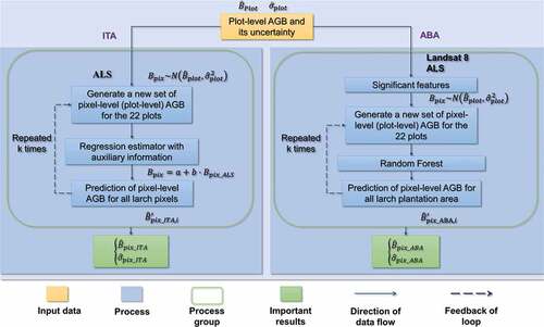
where ${\hat{B}}_{pix\mathrm{\_}ABA,i}^{\prime }$ represents the pixel-level AGB of the i^th simulation based on ABA, k is the number of MC simulations (k = 5000), ${\hat{B}}_{pix\mathrm{\_}ABA}$ represents the pixel-level AGB based on ABA, that is, average of the pixel-level AGB of k simulations based on ABA; ${\hat{\sigma }}_{pix\mathrm{\_}ABA}$ is the estimated standard deviation of the pixel-level AGB based on ABA. The flowchart of the MC process of pixel-level AGB estimation based on ITA and ABA is shown in Figure 3. All the MC simulations in this study were conducted in R 4.0.3 version (R Core Team 2020).

Figure 3. The MC procedures of pixel-level AGB estimation based on ITA and ABA. The pixel-level AGB and its uncertainty based on ITA (${\hat{B}}_{pix\mathrm{\_}ITA}$, ${\hat{\sigma }}_{pix\mathrm{\_}ITA}$) was estimated with the regression estimator of SRS with auxiliary information and MC procedure; the pixel-level AGB and its uncertainty based on ABA (${\hat{B}}_{pix\mathrm{\_}ABA}$, ${\hat{\sigma }}_{pix\mathrm{\_}ABA}$) was estimated with the random forest and MC procedure.

2.3.4. Stand-level AGB estimation and its uncertainty

The stand-level AGB was the summation of pixel-level AGB of each sub-compartment, the smallest forest management unit in China. According to the error propagation formula (Merrin 2017), the stand-level AGB (${\hat{B}}_{st}$) and its uncertainty (${\hat{\sigma }}_{st}^2$) were estimated using equation (18)(18) $\begin{array}{c}\left\{\begin{array}{c}{\hat{B}}_{st}=\sum _{j=1}^m{\hat{B}}_{pix\mathrm{\_}i,j}\\ {\hat{\sigma }}_{st}^2=\sqrt{\sum _{j=1}^m{\hat{\sigma }}_{pix\mathrm{\_}i,j}^2}\end{array}\right.\end{array}$(18) , with the assumption of independent pixels.

(18) $\begin{array}{c}\left\{\begin{array}{c}{\hat{B}}_{st}=\sum _{j=1}^m{\hat{B}}_{pix\mathrm{\_}i,j}\\ {\hat{\sigma }}_{st}^2=\sqrt{\sum _{j=1}^m{\hat{\sigma }}_{pix\mathrm{\_}i,j}^2}\end{array}\right.\end{array}$(18)

where i is an index of either ITA or ABA; m represents the total pixel number of a subcompartment; ${\hat{B}}_{pix\mathrm{\_}i,j}$ represents the estimated j^th pixel-level AGB based on either ITA or ABA; ${\hat{\sigma }}_{pix\mathrm{\_}i,j}$ represents the estimated standard deviation of the j^th pixel-level AGB based on either ITA or ABA. Then, the distribution maps of stand-level AGB and its uncertainty based on ITA and ABA were generated and compared.

3. Results

3.1. Estimation of individual tree parameters

Based on ULS-BLS data, the four ITCD algorithms (i.e. PCS, WS, SRG, and RHCSA) were conducted to delineate individual trees and evaluated using recall (r), precision (p), and F-score at a plot level. Table 3 shows that PCS performed best due to the four algorithms’ highest average r, p, and F-score. The recall indices (r) of WS, SRG, and RHCSA were much lower than the precision indices (p) of the corresponding method, which indicated the three methods had a large number of false negatives (FNs). It was because WS, SRG, and RHCSA were CHM-based ITCD algorithms, which were difficult to detect small trees under canopies. However, according to both r and p values, the PCS method was accurate, which indicated that the undersegmentation decreased effectively, especially for plots with high canopy closure.

Table 3. The accuracy assessment for four ITCD algorithms at plot level

Algorithms	r *	p *	F-score *
PCS	0.64	0.64	0.64
WS	0.46	0.89	0.60
SRG	0.45	0.86	0.58
RHCSA	0.44	0.85	0.57

Note: * represented the average r, p, and F-score of 22 plots. PCS: point cloud segmentation, WS: watershed segmentation; SRG: seeded region growing, RHCSA: region hierarchical cross-sectional analysis (RHCSA).

Table 4 shows that PCS obtained the most 1:1 matched trees (i.e.1595) out of 2451 reference trees and the highest accuracy of DBH despite the lowest accuracy of tree height among the four algorithms. It was because that the point cloud segmentation method could detect more 1:1 matched trees but easily miss the treetops. In contrast, the CHM-based algorithms greatly undersegmented the individual trees, which yielded only about 41% (i.e. WS, SRG, and RHCSA) of 1:1 matched trees.

Table 4. The accuracy assessment of individual tree parameters based on different ITCD algorithms

Algorithm	N	Parameter	R^2	RMSE	rRMSE(%)
PCS	1595	DBH	0.97	1.24	7.40
		H	0.78	2.78	17.87
WS	1021	DBH	0.95	1.74	10.44
		H	0.93	1.81	11.67
SRG	1028	DBH	0.95	1.81	10.85
		H	0.93	1.81	11.64
RHCSA	995	DBH	0.95	1.86	11.12
		H	0.91	2.41	15.52

Note: N presented 1:1 matched trees, DBH presented diameter at breast height (cm), H presented tree height (m).

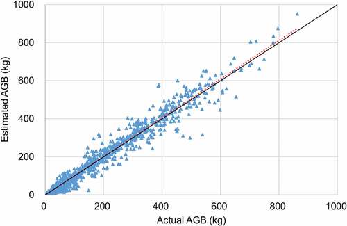
Considering the number of 1:1 matched trees and the accuracies of DBH and tree height, we applied the PCS algorithm to delineate individual trees and calculate the AGB at an individual tree level by equation (1)(1) $\begin{array}{c}\left\{\begin{array}{c}\begin{array}{c}\mathrm{l}\mathrm{n}{W}_s=-4.5363+1.7008\cdot lnD+1.4804\cdot lnH\\ \mathrm{l}\mathrm{n}{W}_b=-3.3632+2.6728\cdot lnD-0.7052\cdot lnH\end{array}\\ \mathrm{l}\mathrm{n}{W}_f=-2.2879+1.3369\cdot lnD-0.0922\cdot \mathrm{l}\mathrm{n}H\\ ln{W}_a=ln\left(W_s+W_b+W_f\right)\end{array}\right.\end{array}$(1) . Figure 4 also indicates that high accuracy of AGB at an individual tree level (R² = 0.97, RMSE = 28.58 kg, rRMSE = 21.13%) was obtained by PCS algorithm and ULS-BLS data. Thus, PCS was applied in the subsequent procedures.

Figure 4. The relationship of estimated and actual individual tree AGB based on PCS algorithm and ULS-BLS data (unit: kg). Note: the solid black line is a 1:1 line, and the red dot is the regression line.

3.2. Plot-level AGB estimation and its uncertainty

3.2.1. Plot-level AGB estimation

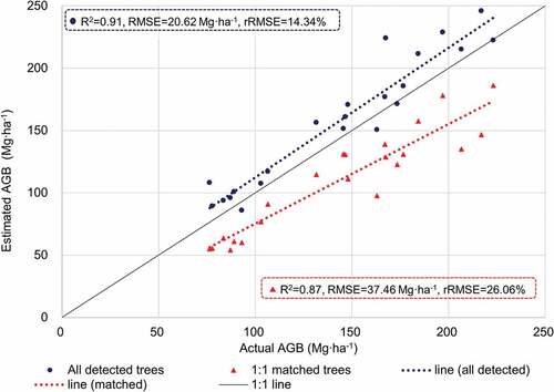
The plot-level AGBs of 22 larch plantation plots could be aggregated by the individual tree-level AGB of all detected trees or the 1:1 matched trees using the PCS algorithm and ULS-BLS data. Figure 5 shows that the plot-level AGB based on all detected trees had much higher accuracy (about 4% higher R², 16.84 Mg·ha⁻¹ lower RMSE, and 11.72% lower rRMSE) than that based on only 1:1 matched trees. The plot-level AGB calculated by 1:1 matched trees suffered underestimation since many trees cannot be matched to the reference trees. Although the plot AGB aggregated by all detect trees slightly overestimated the actual AGB, especially for the large trees, the estimates still had high accuracy (R² = 0.91, RMSE = 20.62 Mg·ha⁻¹, rRMSE = 14.34%). Since we explored the uncertainty based on the ITCD algorithm, the plot-level AGB aggregated by all detected trees was applied in this study.

Figure 5. Relationship between plot-level actual AGB and estimated AGB aggregated by all detected trees (blue dot) and 1:1 matched trees (red triangle) using PCS and ULS-BLS. The accuracy indices of estimated AGB aggregated by all detected trees and 1:1 matched trees are showed in the blue and red dash rectangle, respectively.

3.2.2. Uncertainty of plot-level AGB estimation

To investigate the uncertainty of plot-level AGB estimation, we acquired the standard error of DBH and tree height residuals based on 1:1 matched trees of 1595 detected by the PCS algorithm and ULS-BLS. Use 70% of the 1:1 data to build the model and 30% of the data to verify the accuracy of the DBH model and H model. Table 5 lists the details of the linear models of DBH and tree height fitted by the corresponding actual data.

Table 5. The linear models of DBH and tree height fitted by the corresponding actual data

Model	N	Estimates		R^2	Residual standard error (RSE)
		Intercept	Slope
DBH (cm)	1595	−0.78	0.95	0.98	1.22
Tree height (m)	1595	3.2	0.84	0.79	2.56

According to the DBH and tree height models, we assumed the residual of DBH and tree height followed normal distributions with the mean of zero and the variance of the square of the corresponding RSE, that is, ${\epsilon }_{d^{\prime }}\sim \left(0,{1.22}^2\right)$ and ${\epsilon }_h^{\prime }\sim \left(0,{2.56}^2\right)$,where ${\epsilon }_d^{\prime }$ and ${\epsilon }_h^{\prime }$ were the new residuals of the DBH and tree height, respectively. The plot-level AGB and its uncertainty were obtained using Monte Carlo simulation of 5000 times. The MC simulation of 5000 was sufficient and applied for plot-level AGB estimation since the plot-level AGB estimates and its uncertainty stabilized at 245.69 Mg·ha⁻¹ and 5.25 Mg·ha⁻¹, respectively, after about 2400 simulations. Taking Plot 1 as an example, supplementary figure 1 represented how the plot-level AGB estimates and its uncertainty change with the increase of MC simulation number.

The average and standard deviation of 5000 values were the plot-level AGB estimate and uncertainty considering the errors derivated from the estimates of individual tree parameters based on ITA. Table 6 shows that the estimates of plot-level AGB covered an extensive range (87.34 ~ 245.69 Mg·ha⁻¹) with the standard deviation of 51.38 Mg·ha⁻¹. In contrast, the uncertainty range was relatively small (1.96 to 5.25 Mg·ha⁻¹) with a standard deviation of 1.11 Mg·ha⁻¹.

Table 6. The estimates of plot-level AGB and its uncertainty after MC simulation (Unit: Mg·ha⁻¹)

Estimate	Min	Mean	Median	Max	Standard deviation
Plot-level AGB (${\hat{B}}_{plot}$)	87.34	158.16	158.65	245.69	51.38
Uncertainty (${\hat{\sigma }}_{plot}$)	1.96	3.64	3.97	5.25	1.11

3.3. Pixel-level AGB estimation and its uncertainty using ITA and ABA

3.3.1. Extraction of larch plantations

The larch plantations of Maoershan Forest Farm were extracted using an RF classifier. The RF classifier obtained a high overall accuracy (OA) of 99.45%, and the producer’s accuracy (PA) and user’s accuracy (UA) of larch plantations were 96.25% and 97.47%, respectively. Then, all the larch plantations of Maoershan were extracted using the trained RF classifier (see Supplementary figure 2.).

3.3.2. Pixel-level AGB estimation and its uncertainty using ITA

The DBH-tree height model at the individual tree level (equation (19)(19) $\begin{array}{c}lnD=1.30+0.091\cdot H\end{array}$(19) ) was established using field measurements to estimate the DBH of individual trees derived from ALS. The R², RMSE, and rRMSE were 0.87, 4.08 cm, and 24.06%, respectively.

(19) $\begin{array}{c}lnD=1.30+0.091\cdot H\end{array}$(19)

The individual tree AGB based on ALS data was calculated using equation (1)(1) $\begin{array}{c}\left\{\begin{array}{c}\begin{array}{c}\mathrm{l}\mathrm{n}{W}_s=-4.5363+1.7008\cdot lnD+1.4804\cdot lnH\\ \mathrm{l}\mathrm{n}{W}_b=-3.3632+2.6728\cdot lnD-0.7052\cdot lnH\end{array}\\ \mathrm{l}\mathrm{n}{W}_f=-2.2879+1.3369\cdot lnD-0.0922\cdot \mathrm{l}\mathrm{n}H\\ ln{W}_a=ln\left(W_s+W_b+W_f\right)\end{array}\right.\end{array}$(1) . The ALS-based plot-level (i.e. pixel-level) AGB was obtained by summating individual tree AGB and then dividing by pixel or plot area (30 m × 30 m). The pixel-level AGB was estimated using the regression estimator of simple random sample (SRS) with auxiliary information, considering the plot-level (i.e. pixel-level) AGB based on ULS-BLS data (i.e. ${\hat{B}}_{plot}$) as response variable and the ALS-based plot-level (i.e. pixel-level) AGB as auxiliary information. After 5000 MC simulation, pixel-level AGB based on ITA (i.e. ${\hat{B}}_{pix\mathrm{\_}ITA}$) was estimated. 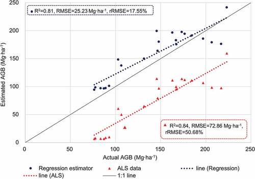Figure 6 shows the comparison of accuracies of estimated pixel-level AGB based on ALS data ($B_{pix\mathrm{\_}ALS}$) and that adjusted by the regression estimator (${\hat{B}}_{pix\mathrm{\_}ITA}$) for the 22 plots of larch plantations. It indicated that the accuracy of pixel-level AGB was significantly improved after adjusting with the regression estimator according to RMSE (from 72.86 to 25.23 Mg·ha⁻¹) and rRMSE (from 50.67% to 17.55%), and the underestimation of ALS-based pixel-level AGB was efficiently reduced.

Figure 6. Comparison of accuracies of pixel-level AGB estimates obtained by ALS data ($B_{pix\mathrm{\_}ALS}$) and adjusted by the regression estimator (${\hat{B}}_{pix\mathrm{\_}ITA}$) for the 22 plots of larch plantations (unit: Mg·ha⁻¹). The accuracy indices of $B_{pix\mathrm{\_}ALS}$ and ${\hat{B}}_{pix\mathrm{\_}ITA}$ are showed in the red and blue dash rectangle, respectively.

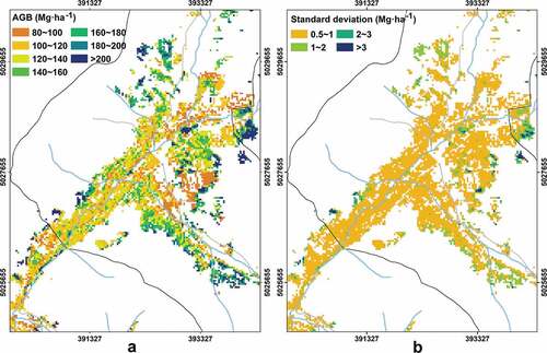
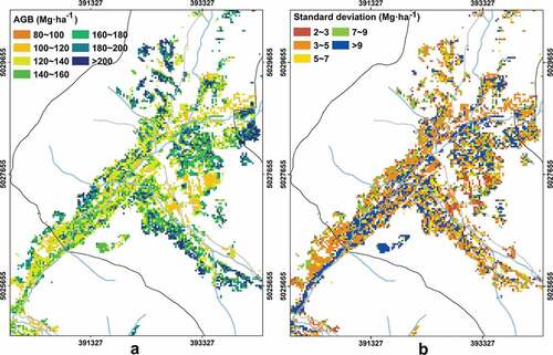
The pixel-level AGB estimates of larch plantations in Maoershan Forest Farm based on ITA ranged from 90.42 to 583.35 Mg·ha⁻¹ with a mean of 129.66 Mg·ha⁻¹, and its standard deviation ranged from 0.65 to 7.58 Mg·ha⁻¹ with a mean of 0.88 Mg·ha⁻¹. Figure 7 only presents the distribution of pixel-level AGB estimates and its uncertainty of larch plantations around the Xinken District that is located in the center area of Maoershan since the district possessed the most extensive larch plantations. This area was dominated by the AGB estimates and its uncertainty less than 180 Mg·ha⁻¹ (Figure 7(a)) and less than 1 Mg·ha⁻¹ (Figure 7 (b)), respectively. The high uncertainty was mainly located at the pixels with high AGB values.

Figure 7. The spatial distribution of pixel-level AGB estimates (${\hat{B}}_{pix\mathrm{\_}ITA}$) (a) and its uncertainty (${\hat{\sigma }}_{pix\mathrm{\_}ITA}$) (b) of larch plantations based on ITA around Xinken District. Xinken District was dominated by the AGB estimates and its uncertainty less than 180 Mg·ha⁻¹ and less than 1 Mg·ha⁻¹, respectively.

3.3.3. Pixel-level AGB estimation and its uncertainty using ABA

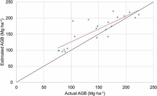
The two-step feature selection was applied in this study. 78 out of 200 features were primarily selected using Pearson correlation coefficient, and then ten significant features with the variable importance of RF greater than 1000 were finally determined. Seven elevation features and three spectral features were selected from ALS data and Landsat 8 imagery, respectively (shown in supplementary table 2 and 3), indicating the significance of active and passive remotely sensed data in AGB estimation. An area-based AGB model was established using the RF algorithm and selected features. Figure 8 presents the relationship between pixel-level estimated and actual AGB of the 22 plots based on ABA, which indicated a lower accuracy (R² = 0.72, RMSE = 30.29 Mg·ha⁻¹, rRMSE = 21.07%) than that based on ITA (R² = 0.81, RMSE = 25.23 Mg·ha⁻¹, rRMSE = 17.55% showed in Figure 6). The model slightly overestimated the AGB values less than 150 Mg·ha⁻¹.

Figure 8. Relationship between pixel-level estimated and actual AGB of the 22 plots based on ABA. (unit: Mg·ha⁻¹).

The pixel-level AGB estimates of larch plantations in Maoershan Forest Farm based on ABA ranged from 100.35 to 220.89 Mg·ha⁻¹ with a mean of 144.38 Mg·ha⁻¹, and its uncertainty ranged from 2.02 Mg·ha⁻¹ to 14.70 Mg·ha⁻¹ with a mean of 6.41 Mg·ha⁻¹. The area around Xinken District was dominated by AGB estimates and its uncertainty less than 180 Mg·ha⁻¹ (Figure 9(a)) and greater than 3 Mg·ha⁻¹ (Figure 9(b)), respectively. ABA obtained a higher standard deviation of estimated AGB than ITA, indicating more significant spatial uncertainty.

Figure 9. The spatial distribution of pixel-level AGB estimates (${\hat{B}}_{pix\mathrm{\_}ABA}$) (a) and its uncertainty (${\hat{\sigma }}_{pix\mathrm{\_}ABA}$) (b) of larch plantations based on ABA around Xinken District. Xinken District was dominated by AGB estimates and its uncertainty less than 180 Mg·ha⁻¹ and greater than 3 Mg·ha⁻¹, respectively.

3.4. Stand-level AGB estimation and its uncertainty using ITA and ABA

At stand-level, the range of AGB values in Maoershan based on ITA was 90.66 — 567.85 Mg·ha⁻¹ with a mean of 124.60 Mg·ha⁻¹; whereas the range of AGB values based on ABA was 101.22 — 215.33 Mg·ha⁻¹ with a mean of 138.38 Mg·ha⁻¹. For the areas along the road in Xinken District, the estimates of AGB tended to be higher using ABA than those obtained by ITA (see Supplementary figure 3). Although the averages of AGB based on ITA and AGB were similar, ITA provided a more refined detailed distribution and higher variation of AGB than ABA (Supplementary figure 3 (a) vs. (b)).

For spatial uncertainty, the range of stand-level AGB in Maoershan based on ITA was 0.65 — 27.3 Mg·ha⁻¹ with a mean of 2.60 Mg·ha⁻¹. On the other hand, ABA provided a range of 9.11 — 209.89 Mg·ha⁻¹ with a mean of 37.15 Mg·ha⁻¹ for stand-level AGB uncertainty, almost 14 times higher than the mean obtained by ITA. Most areas around Xinken District had a much larger standard deviation (>14 Mg·ha⁻¹) using ABA than ITA, which indicated ITA tended to yield a more stable AGB estimation than ABA (see Supplementary figure 4).

4. Discussion

4.1. Individual tree parameters estimation

An accurate individual tree crown delineation algorithm is a basis and prerequisite for the precise forest structure (Næsset et al. 2016; Korpela et al. 2007). In this study, four individual tree delineation algorithms (PCS, WS, SRG, and RHCSA) were applied to delineate the individual tree crown using ULS-BLS data, but the accuracies were much lower than other studies (Yang et al. 2019; Lu et al. 2014). For example, Li et al. (2012) reported an average F-score of 0.9 for an average tree density of 400 trees·ha⁻¹ using field data as a reference. Tao et al. (2015) reported an average F-score of 0.87 for three forest types (i.e. conifers, broadleaf, and mixed) using manual delineation data as ground truth. The average tree density for conifers, broadleaf, and mixed forest were 314 trees·ha⁻¹, 278 trees·ha⁻¹, and 397 trees·ha⁻¹, respectively. The low F-score (i.e. 0.64 based on PCS) obtained in this study maybe because (1) the tree density and canopy closure are pretty high in the sample plots of larch plantations located in natural secondary forests, with an average of 1265 trees·ha⁻¹ and 0.83, respectively. (2) All the locations of trees were recorded with RTK in the field, of which the dense canopy greatly influenced signals. The positioning accuracy could be decreased. In addition, the locations of trees were measured at or near the trunks in the field from an upward view, whereas most ITCD algorithms (e.g. WS, SRG, RHCSA) positioned the trees at treetops from an overhead perspective. The tree locations detected from different perspectives and the high tree density easily resulted in the mismatches in accuracy assessment. (3) we conducted a rigorous accuracy assessment from an accuracy indices perspective. The F-score was calculated based on 1:1 matched trees, which were determined by not only locations but DBH differences and tree height differences. Then, a small part of matched trees with the absolute values of external studentized residuals greater than three were considered outliers and removed. The strict conditions of matched trees limited the accuracy to some degree. However, the individual tree AGB based on the 1:1 matched trees was relatively accurate (R² = 0.97, RMSE = 28.58 kg, rRMSE = 21.13%).

Similar to the previous studies, compared to the PCS algorithm, the three CHM-based methods (e.g. WS, SRG, RHCSA) had weaknesses in detecting small trees, especially for the forests with high canopy closure (Reitberger, Krzystek, and Stilla 2009; Yang et al. 2019). The PCS algorithm performed better since it considers tree trunks as seeds. However, the tree height estimated using PCS had low accuracy (R² = 0.78, RMSE = 2.78 m, rRMSE = 17.87%) because the PCS detected some small trees from the bottom-up perspective, of which treetops were overlapped within the canopy and not detected accurately for tree height estimation. Another reason for the low accuracy is the discontinuous point cloud for some trees. The major shortcoming of BLS system is the lack of points for the upper part of trees (Huang et al. 2019). Since the limited vertical field of view of the BLS system (−15°~15°) and penetration ability of ULS used in this study, the point clouds of some trees are not continuous around the middle height within the canopy, especially for the tall trees (see Supplementary figure 5). This phenomenon significantly decreased the accuracy of individual tree parameters estimation. With the improvement of the backpack LiDAR instrument, this problem could be alleviated to some extent in the future.

4.2. The AGB estimation and its uncertainty of two approaches

Based on the stable estimates of plot-level AGB, we bridged the field and satellite-based measurements using both individual tree-based and area-based approaches, taking larch plantations as an example. We only considered larch plantations in this study mainly because (1) Larix olgensis Henry is one of the most notable afforestation tree species in Heilongjiang Province with about 45% of 36% of the total plantation area and standing volume, respectively (Gao, Dong, and Li 2017; State Forestry Administration 2014). It is also a critical timber and carbon sink tree species with high economic and ecological values due to the outstanding abilities of natural pruning and survival. (2) upscaling procedure from field to satellite measurements based on ITA involves many critical steps or factors that could cause errors, including ITCD, individual tree parameter estimation, individual tree species classification, AGB allometric equations, and so on. Although the ITCD algorithms have been dramatically developed with the evolution of LiDAR data in recent years (Zhen, Quackenbush, and Zhang 2016), the individual tree species classification is still a challenging task, especially for boreal forests (Dalponte et al. 2013). The current study mainly considered the uncertainty of individual tree parameter estimates of larch plantations derived from ITCD and focused on comparing ITA and ABA within the upscaling procedure. The AGB estimation of natural secondary forests (NSFs) would incorporate the individual tree species classification, which significantly complicates the entire procedure and is seriously considered in future research.

Data saturation in Landsat series satellite imagery could easily result in the underestimation of AGB, lower the accuracy, and increase the uncertainties of AGB estimation (Lu et al. 2014). Currently, incorporating LiDAR data provided a potential solution to data saturation in Landsat data, widely recognized in the remote sensing field (e.g. Mean et al. 1999; Lu et al. 2012; Du et al. 2021). With the richness of remotely sensed data, AGB could be estimated at either a more delicate scale (e.g. individual tree level) or a coarser scale (e.g. stand-level) based on ITA and ABA. However, the effect of these two approaches on reducing data saturation has not been fully explored, especially in multi-scale AGB estimation with multi-source remotely sensed data. We compared the histogram of pixel-level AGB estimates and their uncertainties with ITA and ABA (Figure 10). ITA and ABA varied considerably on the distributions of AGB values. The AGB estimates based on ABA were mainly concentrated on the range of 100 — 160 Mg·ha⁻¹, whereas those based on ITA were distributed along with all the intervals. The none of small AGB values (less than 100 Mg·ha⁻¹) estimated by ABA indicated that ABA suffered from overestimating low AGB values, a typical characteristic of data saturation (Zhao et al. 2016a). Based on ABA and Landsat 8, Zhao et al. (2016) reported the AGB saturation values of pine and Chinese fir forests as 159 and 143 Mg·ha⁻¹, respectively, which were lower than the max AGB value (around 200 Mg·ha⁻¹) in this study due to the different forest types and data sources. Although the incorporation of LiDAR increased the AGB saturation of larch plantations (sensitive to the AGB values greater than 180 Mg·ha⁻¹), it was still less sensitive to the AGB values less than 100 Mg·ha⁻¹. On the other hand, the ITA estimated a much wider range of AGB values than the ABA. For ITA, the AGB estimates less than 100 Mg·ha⁻¹ and greater than 180 Mg·ha⁻¹ accounted for 21% and 10%, respectively (Figure 10 (a)). Thus, the ITA effectively eliminated the overestimation of small AGB values caused by ABA.

Figure 10. The histogram of pixel-level (a) AGB estimates and (b) its uncertainties with ITA and ABA. The ITA yielded a much wider range of AGB estimates and lower uncertainties than the ABA.

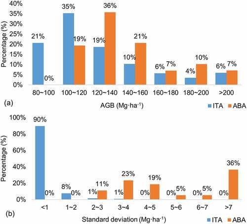
The difference became even more apparent in uncertainty than AGB values (Figure 10(b)). The most pixels (about 90%) based on ITA had relatively low uncertainties with a standard deviation less than 1 Mg·ha⁻¹, whereas the ABA yielded a much larger (>2 Mg·ha⁻¹) uncertainty than ITA. The uncertainty based on ABA mainly focused on the ranges of 3 — 4 Mg·ha⁻¹ and >7 Mg·ha⁻¹, accounting for 23% and 36% of total pixels, respectively. It is worth noticing that about 65% of the pixels had a standard deviation greater than 4 Mg·ha⁻¹ based on ABA, which supported and explained the spatial distributions represented in Figures 7, 9, and supplementary figure 4. This study found that the individual tree approach obtained higher accuracy (R² = 0.81, RMSE = 25.23 Mg·ha⁻¹, rRMSE = 17.55%) and much lower uncertainty (<2 Mg·ha⁻¹ uncertainty) than area-based approach (R² = 0.72, RMSE = 30.29 Mg·ha⁻¹, rRMSE = 21.07%, >2 Mg·ha⁻¹ uncertainty) in estimating pixel-level AGB, which is consistent with the estimates of other forest attributes in previous studies (e.g. Breidenbach et al. 2010; Peuhkurinen et al. 2007). This is because the ITA tends to obtain higher accuracy than ABA in less complex forests or plantations (Xu et al. 2014), have sufficient insight into tree-level details and could easily understand the uncertainties at various spatial scales (Xu et al. 2018).

4.3. Wall-to-wall AGB predictions of two approaches

Currently, the method of wall-to-wall AGB predictions is dominated by ABA due to feasibility and applicability for a large area (e.g. Su et al. 2016; Zhang et al. 2019; Du et al. 2021). This study proposed a framework for generating wall-to-wall AGB predictions of larch plantations based on ITA. To compare with ABA, we applied the pixel as the smallest unit of wall-to-wall AGB predictions with ITA instead of an individual tree used in previous studies (e.g. Qiu et al. 2019; Zhao, Popescu, and Nelson 2009). The 22 sample plots that exactly matched the pixel of Landsat 8 were designed as a “bridge” between an individual tree and the smallest unit (i.e. pixel) of wall-to-wall AGB predictions to avoid geolocation mismatching between remote sensing data and field measurements. The wall-to-wall AGB predictions based on ITA were generated using the regression estimator with auxiliary information (i.e. the ALS-based pixel-level AGB estimates). The ALS-based pixel-level AGB of the entire larch plantation area was adjusted or improved by the pixel-level AGB estimated by ULS-BLS data in the sample plots. Thus, the pixel-level AGB estimated by ULS-BLS data was the variable of interest for the entire study area. However, this study had to suffer from the insufficient sample plots since another part of field plots were severely destroyed by the three typhoons (i.e. Typhoon Bavi, Maysak, and Haishen) transitted Maorshan Forest Farm from August 27^th to September 10^th of 2020. Even though the plot size (i.e. 22 plots) is limited in this study, the samples of individual trees (i.e. 2451) are sufficient, which reflects another advantage of ITA approach. The frameworks of upscaling AGB estimates based on both ITA and ABA approaches performed successfully and could be applied for other plantations in the future.

5. Conclusions

Traditionally, it is suitable to apply an area-based approach for large-scale AGB estimation and an individual tree approach for fine AGB mapping, which indicates the two approaches conflict to a certain extent. However, this study investigated the nondestructive AGB estimations of larch plantations using both ITA and ABA and scaled up the AGB estimates, and their spatial uncertainties from an- individual tree- to stand-level based on multi-source remotely sensed data. We found that the PCS algorithm outperformed CHM-based ITCD algorithms for the plots with high tree density (about 1265 trees/ha) and obtained a high accuracy of individual tree AGB estimates (R² = 0.97, RMSE = 28.58 kg, rRMSE = 21.13%). When estimating AGB based on ITA, it is more appropriate to aggregate all detected trees into the plot-level AGB estimation than only considering 1:1 matched trees. The average plot-level AGB estimates of larch plantations and the uncertainty based on Monte Carlo simulation were 158.16 and 3.64 Mg·ha⁻¹, respectively. The average pixel-level AGB of larch plantations in Maorshan Forest Farm estimated by ITA and ABA were very similar, 129.66 Mg·ha⁻¹ and 144.38 Mg·ha⁻¹, respectively. ITA yielded a higher accuracy of the pixel-level AGB estimates and lower spatial uncertainties of pixel-level and stand-level AGB estimates than ABA. The ITA efficiently eliminated the overestimation of low AGB values that commonly occurred in ABA.

The growing demand for fine AGB mapping at large-scale calls for more accurate and efficient AGB estimations at multi-scales. This study contributes to the development of an upscaling framework for AGB estimation based on individual tree detection techniques, as well as a comparison of the effects of ITA and ABA on the pixel- and stand-level AGB estimates and spatial uncertainty. The frameworks based on both ITA and ABA could be applied for other plantations or uncomplex forests. This study also highlights the significance of understanding and quantifying multi-scale spatial uncertainties during AGB estimations. More complex natural forests, on the other hand, necessitate a more comprehensive MC simulation that takes into account more factors such as individual tree crown delineation, tree species classification, and individual tree parameter estimations, all of which could be investigated further in the future. ITA would provide an appealing and promising option for accurate quantification of forest carbon, precise forest monitoring and protection, and sustainable forest management in the future with the continued development of the ITCD algorithm and the quantification of errors.

Disclosure statement

No potential conflict of interest was reported by the author(s).

Data availability statement

The data that support the findings of this study are openly available in [figshare] at [10.6084/m9.figshare.17705627.v1]. The reference data are available on request from the corresponding author, (Y.Z).

Additional information

Funding

This research was funded by the National Natural Science Foundation of China “Multi-scale forest aboveground biomass estimation and its spatial uncertainty analysis based on individual tree detection techniques” 32071677; “The Fundamental Research Funds for the Central Universities,” 2572020BA05, 2572019CP15. This study was also funded by the research fund of China Scholarship Council (CSC-No. 202006605008).

References

- Angelsen, A. 2009. Realising REDD+: National Strategy and Policy Options. Bogor: Center for International Forestry Research (CIFOR).
- Arun, K. S., T. S. Huang, and S. D. Blostein. 1987. “Least-squares Fitting of Two 3-D Point Sets.” IEEE Transactions on Pattern Analysis Machine Intelligence 5 (5): 698–700. doi:10.1109/TPAMI.1987.4767965.
- Bellman, R. E. 1961. Adaptive Control Processes. Princeton: Princeton University Press.
- Besl, P. J., and H. D. Mckay. 1992. “A Method for Registration of 3-D Shapes.” IEEE Transactions on Pattern Analysis Machine Intelligence 14 (2): 239–256. doi:10.1117/12.57955.
- Breidenbach, J., E. Næsset, V. Lien, T. Gobakken, and S. Solberg. 2010. “Prediction of Species Specific Forest Inventory Attributes Using a Nonparametric Semi-individual Tree Crown Approach Based on Fused Airborne Laser Scanning and Multispectral Data.” Remote Sensing of Environment 114 (4): 911–924. doi:10.1016/j.rse.2009.12.004.
- Cao, L., J. Pan, R. Li, J. Li, and Z. Li. 2018. “Integrating Airborne LiDAR and Optical Data to Estimate Forest Aboveground Biomass in Arid and Semi-arid Regions of China.” Remote Sensing 10 (4): 532. doi:10.3390/rs10040532.
- Chen, Q. 2013. “LiDAR Remote Sensing of Vegetation Biomass.“ In Remote Sensing of Natural Resources, edited by Guangxing Wang, Qihao Weng, 399-420. Boca Raton: Taylor & Francis Series in Remote Sensing Applications.
- Chen, Q., D. Baldocchi, P. Gong, and M. Kelly. 2006. “Isolating Individual Trees in a Savanna Woodland Using Small Footprint Lidar Data.” Photogrammetric Engineering Remote Sensing 72 (8): 923–932. doi:10.14358/PERS.72.8.923.
- Chen, J. M., and T. A. Black. 1991. “Measuring Leaf Area Index of Plant Canopies with Branch Architecture.” Agricultural Forest Meteorology 57 (1–3): 1–12. doi:10.1016/0168-1923(91)90074-Z.
- Chen, Q., G. V. Laurin, and R. Valentini. 2015. “Uncertainty of Remotely Sensed Aboveground Biomass over an African Tropical Forest: Propagating Errors from Trees to Plots to Pixels.” Remote Sensing of Environment 160: 134–143. doi:10.1016/j.rse.2015.01.009.
- Chen, Q., R. E. McRoberts, C. Wang, and P. J. Radtke. 2016. “Forest Aboveground Biomass Mapping and Estimation across Multiple Spatial Scales Using Model-based Inference.” Remote Sensing of Environment 184: 350–360. doi:10.1016/j.rse.2016.07.023.
- Cohen, R., J. Kaino, J. A. Okello, J. O. Bosire, J. G. Kairo, M. Huxham, and M. Mencuccini. 2013. “Propagating Uncertainty to Estimates of Above-ground Biomass for Kenyan Mangroves: A Scaling Procedure from Tree to Landscape Level.” Forest Ecology Management 310: 968–982. doi:10.1016/j.foreco.2013.09.047.
- Dalponte, M., H. O. Ørka, T. Gobakken, D. Gianelle, and E. Næsset. 2013. “Tree Species Classification in Boreal Forests with Hyperspectral Data.” IEEE Transactions on Geoscience Remote Sensing 51 (5): 2632–2645. doi:10.1109/TGRS.2012.2216272.
- Dong, L. 2015. “Developing individual and stand-level biomass equations in northeast China forest area.“ PhD diss., Northeast Forestry University.
- Du, C., W. Fan, Y. Ma, H. Jin, and Z. Zhen. 2021. “The Effect of Synergistic Approaches of Features and Ensemble Learning Algorithms on Aboveground Biomass Estimation of Natural Secondary Forests Based on ALS and Landsat 8.” Sensors 21 (17): 5974. doi:10.3390/s21175974.
- Ene, L., E. Næsset, and T. Gobakken. 2012. “Single Tree Detection in Heterogeneous Boreal Forests Using Airborne Laser Scanning and Area-based Stem Number Estimates.” International Journal of Remote Sensing 33 (16): 5171–5193. doi:10.1080/01431161.2012.657363.
- Fang, F., J. Im, J. Lee, and K. Kim. 2016. “An Improved Tree Crown Delineation Method Based on Live Crown Ratios from Airborne LiDAR Data.” GIScience & Remote Sensing 53 (3): 402–419. doi:10.1080/15481603.2016.1158774.
- Fu, L., Q. Liu, H. Sun, Q. Wang, Z. Li, E. Chen, Y. Pang, X. Song, and G. Wang. 2018. “Development of a System of Compatible Individual Tree Diameter and Aboveground Biomass Prediction Models Using Error-in-variable Regression and Airborne LiDAR Data.” Remote Sensing 10 (2): 325. doi:10.3390/rs10020325.
- Gao, H., L. Dong, and F. Li. 2017. “Modeling Variation in Crown Profile with Tree Status and Cardinal Directions for Planted Larix Olgensis Henry Trees in Northeast China.” forests 8 (5): 139. doi:10.3390/f8050139.
- Gertner, G., X. Cao, and H. Zhu. 1995. “A Quality Assessment of A Weibull Based Growth Projection System.” Forest Ecology Management 71 (3): 235–250. doi:10.1016/0378-1127(94)06104-Q.
- Gertner, G., P. Parysow, and B. Guan. 1996. “Projection Variance Partitioning of a Conceptual Forest Growth Model with Orthogonal Polynomials.” Forest Science 42 (4): 474–486. doi:10.1016/S0378-1127(96)03878-9.
- Gleason, C. J., and J. Im. 2011. “A Review of Remote Sensing of Forest Biomass and Biofuel: Options for Small-Area Applications.” GIScience & Remote Sensing 48 (2): 141–170. doi:10.2747/1548-1603.48.2.141.
- Goutte, C., and E. Gaussier. 2005. “A Probabilistic Interpretation of Precision, Recall and F-score, with Implication for Evaluation.” In European Conference on Information Retrieval (ECIR) 2005: Advances in Information Retrieval, edited by D. E. Losada and J. M. Fernández-Luna, 345–359. Berlin: Springer. 10.1007/978-3-540-31865-1_25.
- Hamraz, H., M. A. Contreras, and J. Zhang. 2017. “Vertical Stratification of Forest Canopy for Segmentation of Understory Trees within Small-footprint Airborne LiDAR Point Clouds.” ISPRS Journal of Photogrammetry Remote Sensing 130: 385–392. doi:10.1016/j.isprsjprs.2017.07.001.
- Hao, Y., F. R. Widagdo, X. Liu, Y. Liu, L. Dong, and F. Li. 2022. “A Hierarchical Region-merging Algorithm for 3D Segmentation of Individual Trees Using UAV-LiDAR Point Clouds.“ IEEE Transactions on Geoscience Remote Sensing 40: 1558–0644. doi: 10.1109/TGRS.2021.3121419.
- Hao, Y., Z. Zhen, F. Li, and Y. Zhao. 2019. “A Graph-based Progressive Morphological Filtering (GPMF) Method for Generating Canopy Height Models Using ALS Data.” International Journal of Applied Earth Observation and Geoinformation 79: 84–96. doi:10.1016/j.jag.2019.03.008.
- Haralick, R. M. 1974. “A Measure for Circularity of Digital Figures.” IEEE Transactions on Systems, Man, and Cybernetics 4 (4): 394–396. SMC
- Hijmans, R. J. 2022. “Raster: Geographic Data Analysis and Modeling. R Package Version 3.5-15.” https://CRAN.R-project.org/package=raster
- Huang, X., W. Jia, Q. Wang, Y. Zhen, and Y. Liang. 2019. “Study on Individual Tree Factor Extraction of Larix Olgensis in Backpack Lidar.” Forest Engineering 35 (4): 8. Chinese
- Hyyppä, J., O. Kelle, M. Lehikoinen, and M. Inkinen. 2001. “A Segmentation-based Method to Retrieve Stem Volume Estimates from 3-D Tree Height Models Produced by Laser Scanners.” IEEE Transactions on Geoscience Remote Sensing 39 (5): 969–975. doi:10.1109/36.921414.
- Ji, L., G. Zhou, L. Gu, and L. Wang. 2017. “Research Status and Prospects of “REDD+.” World Agriculture 06: 161–167. doi:10.13856/j.cn11-1097/s.2017.06.026.
- Khosravipour, A., A. K. Skidmore, and M. Isenburg. 2016. “Generating Spike-free Digital Surface Models Using LiDAR Raw Point Clouds: A New Approach for Forestry Applications.” International Journal of Applied Earth Observation Geoinformation 52: 104–114. doi:10.1016/j.jag.2016.06.005.
- Koch, B., U. Heyder, and H. Weinacker. 2006. ”Detection of individual tree crowns in airborne lidar data.” Photogrammetric Engineering Remote Sensing 72 (4): 357–63. doi:10.14358/PERS.72.4.357.
- Korpela, I., B. Dahlin, H. Schäfer, E. Bruun, F. Haapaniemi, J. Honkasalo, S. Ilvesniemi, et al. 2007. “Single-tree Forest Inventory Using Lidar and Aerial Images for 3D Treetop Positioning, Species Recognition, Height and Crown Width Estimation.” Paper presented at the Proceedings of ISPRS workshop on laser scanning, September 12-14, 2007, Espoo, Finland.
- Latifi, H., F. E. Fassnacht, J. Müller, A. Tharani, S. Dech, and M. Heurich. 2015. “Forest Inventories by LiDAR Data: A Comparison of Single Tree Segmentation and Metric-based Methods for Inventories of A Heterogeneous Temperate Forest.” International Journal of Applied Earth Observation and Geoinformation 42: 162–174. doi:10.1016/j.jag.2015.06.008.
- Leckie, D., F. Gougeon, D. Hill, R. Quinn, L. Armstrong, and R. Shreenan. 2003. “Combined High-density Lidar and Multispectral Imagery for Individual Tree Crown Analysis.” Canadian Journal of Remote Sensing 29 (5): 633–649. doi:10.5589/m03-024.
- Lee, S. J., J. R. Kim, and Y. S. Choi. 2013. “The Extraction of Forest CO2 Storage Capacity Using High-resolution Airborne Lidar Data.” GIScience & Remote Sensing 50 (2): 154–171. doi:10.1080/15481603.2013.786957.
- Lei, C., C. Ju, T. Cai, X. Jing, X. Wei, and X. Di. 2012. “Estimating Canopy Closure Density and Above-ground Tree Biomass Using Partial Least Square Methods in Chinese Boreal Forests.” Journal of Forestry Research 23 (2): 191–196. doi:10.1007/s11676-012-0232-x.
- Li, W., Q. Guo, M. K. Jakubowski, and M. Kelly. 2012. “A New Method for Segmenting Individual Trees from the Lidar Point Cloud.” Photogrammetric Engineering Remote Sensing 78 (1): 75–84. doi:10.14358/PERS.78.1.75.
- Li, M., J. Im, L. J. Quackenbush, and T. Liu. 2014. “Forest Biomass and Carbon Stock Quantification Using Airborne LiDAR Data: A Case Study over Huntington Wildlife Forest in the Adirondack Park.” IEEE Journal of Selected Topics in Applied Earth Observations Remote Sensing 7 (7): 3143–3156. doi:10.1109/JSTARS.2014.2304642.
- Li, Y., C. Li, M. Li, and Z. Liu. 2019. “Influence of Variable Selection and Forest Type on Forest Aboveground Biomass Estimation Using Machine Learning Algorithms.” forests 10 (12): 1073. doi:10.3390/f10121073.
- Li, W., Z. Niu, X. Liang, Z. Li, N. Huang, S. Gao, C. Wang, and S. Muhammad. 2015. “Geostatistical Modeling Using LiDAR-derived Prior Knowledge with SPOT-6 Data to Estimate Temperate Forest Canopy Cover and Aboveground Biomass via Stratified Random Sampling.” International Journal of Applied Earth Observation Geoinformation 41: 88–98. doi:10.1016/j.jag.2015.04.020.
- Liu, S., F. Cheng, S. Dong, H. Zhao, X. Hou, and X. Wu. 2017. “Spatiotemporal Dynamics of Grassland Aboveground Biomass on the Qinghai-Tibet Plateau Based on Validated MODIS NDVI.” Scientific Reports 7 (1): 1–10. doi:10.1038/s41598-017-04038-4.
- Lu, D., Q. Chen, G. Wang, L. Liu, G. Li, and E. Moran. 2016. “A Survey of Remote Sensing-based Aboveground Biomass Estimation Methods in Forest Ecosystems.” International Journal of Digital Earth 9 (1): 63–105. doi:10.1080/17538947.2014.990526.
- Lu, D., Q. Chen, G. Wang, E. Moran, M. Batistella, M. Zhang, G. V. Laurin, and D. Saah. 2012. “Aboveground Forest Biomass Estimation with Landsat and LiDAR Data and Uncertainty Analysis of the Estimates.” International Journal of Forestry Research 2012: 1–16. doi:10.1155/2012/436537.
- Lu, X., Q. Guo, W. Li, and J. Flanagan. 2014. “A Bottom-up Approach to Segment Individual Deciduous Trees Using Leaf-off Lidar Point Cloud Data.” ISPRS Journal of Photogrammetry Remote Sensing 94: 1–12. doi:10.1016/j.isprsjprs.2014.03.014.
- Manzanera, J. A., A. García-Abril, C. Pascual, R. Tejera, S. Martín-Fernández, T. Tokola, and R. Valbuena. 2016. “Fusion of Airborne LiDAR and Multispectral Sensors Reveals Synergic Capabilities in Forest Structure Characterization.” GIScience & Remote Sensing 53 (6): 723–738. doi:10.1080/15481603.2016.1231605.
- Means, J. E., S. A. Acker, D. J. Harding, J. B. Blair, M. A. Lefsky, W. B. Cohen, M. E. Harmon, and W. A. McKee. 1999. “Use of Large-footprint Scanning Airborne Lidar to Estimate Forest Stand Characteristics in the Western Cascades of Oregon.” Remote Sensing of Environment 67 (3): 298–308. doi:10.1016/S0034-4257(98)00091-1.
- Mehnert, A., and P. Jackway. 1997. “An Improved Seeded Region Growing Algorithm.” Pattern Recognition Letters 18 (10): 1065–1071. doi:10.1016/S0167-8655(97)00131-1.
- Meng, S., Y. Pang, Z. Zhang, W. Jia, and Z. Li. 2016. “Mapping Aboveground Biomass Using Texture Indices from Aerial Photos in a Temperate Forest of Northeastern China.” Remote Sensing 8 (3): 230. doi:10.3390/rs8030230.
- Merrin, J. 2017. Introduction to Error Analysis: The Science of Measurements, Uncertainties, and Data Analysis . CreateSpace Independent Publishing Platform, Version 1.1.
- Montesano, P. M., R. F. Nelson, R. O. Dubayah, G. Sun, B. D. Cook, K. J. R. Ranson, E. Næsset, and V. Kharuk. 2014. “The Uncertainty of Biomass Estimates from LiDAR and SAR across a Boreal Forest Structure Gradient.” Remote Sensing of Environment 154: 398–407. doi:10.1016/j.rse.2014.01.027.
- Næsset, E., and T. Gobakken. 2008. “Estimation of Above-and Below-ground Biomass across Regions of the Boreal Forest Zone Using Airborne Laser.” Remote Sensing of Environment 112 (6): 3079–3090. doi:10.1016/j.rse.2008.03.004.
- Næsset, E., H. O. Ørka, S. Solberg, O. M. Bollandsås, E. H. Hansen, E. Mauya, E. Zahabu, et al. 2016. “Mapping and Estimating Forest Area and Aboveground Biomass in Miombo Woodlands in Tanzania Using Data from Airborne Laser Scanning, TanDEM-X, RapidEye, and Global Forest Maps: A Comparison of Estimated Precision.” Remote Sensing of Environment 175:282–300. doi:10.1016/j.rse.2016.01.006.
- Ometto, J. P., A. P. Aguiar, T. Assis, L. Soler, P. Valle, G. Tejada, D. M. Lapola, and P. Meir. 2014. “Amazon Forest Biomass Density Maps: Tackling the Uncertainty in Carbon Emission Estimates.” Climatic Change 124 (3): 545–560. doi:10.1007/s10584-014-1058-7.
- Ørka, H. O., E. Næsset, and O. M. Bollandsås. 2009. “Classifying Species of Individual Trees by Intensity and Structure Features Derived from Airborne Laser Scanner Data.” Remote Sensing of Environment 113 (6): 1163–1174. doi:10.1016/j.rse.2009.02.002.
- Pang, Y., Z. Li, H. Ju, Q. Liu, L. Si, S. Li, B. Tan, et al. 2016. “LiCHy: CAF’s LiDAR, CCD and Hyperspectral Airborne Observation System.” Remote Sensing 8 (5): 398. doi:10.3390/rs8050398.
- Pebesma, E. 2018. “Simple Features for R: Standardized Support for Spatial Vector Data.” The R Journal 10 (1): 439–446. doi:10.32614/RJ-2018-009.
- Peng, S., and X. Deng. 2017. “A New Method of Whole Least Squares for Four-parameter Solution of Coordinate Transformation.” Surveying Engineering 26 (9): 10–13. doi:10.19349/j.cnki.1006-7949.2017.09.003.
- Peuhkurinen, J., M. Maltamo, J. Malinen, J. Pitkänen, and P. Packalén. 2007. “Preharvest Measurement of Marked Stands Using Airborne Laser Scanning.” Forest Science 53 (6): 653–661. doi:10.1093/forestscience/53.6.653.
- Popescu, S. C. 2007. “Estimating Biomass of Individual Pine Trees Using Airborne Lidar.” Biomass and Bioenergy 31 (9): 646–655. doi:10.1016/j.biombioe.2007.06.022.
- Qiu, P., D. Wang, X. Zou, X. Yang, G. Xie, S. Xu, and Z. Zhong. 2019. “Finer Resolution Estimation and Mapping of Mangrove Biomass Using UAV LiDAR and Worldview-2 Data.” forests 10 (10): 871. doi:10.3390/f10100871.
- R Core Team. 2020. R: A Language and Environment for Statistical Computing. R Foundation for Statistical Computing: Vienna, Austria. URL. https://www.R-project.org/
- Raychaudhuri, S. 2008. “Introduction to Monte Carlo Simulation.” Paper presented at the 2008 Winter simulation conference, December 7-10, Miami, Florida, USA.
- Reitberger, J., P. Krzystek, and U. Stilla. 2009. “Benefit of Airborne Full Waveform Lidar for 3D Segmentation and Classification of Single Trees.” Paper presented at the ASPRS 2009 Annual Conference, Baltimore, Maryland, USA.
- Saatchi, S. S., N. L. Harris, S. Brown, M. Lefsky, E. T. A. Mitchard, W. Salas, B. R. Zutta, et al. 2011. “Benchmark Map of Forest Carbon Stocks in Tropical Regions across Three Continents.” Proceedings of the National Academy of Sciences 108 (24): 9899–9904. doi:10.1073/pnas.1019576108.
- Satoo, T., and H. A. Madgwick. 2012. Forest Biomass. Vol. 6. Dordrecht: Springer Science & Business Media.
- Shettles, M., T. Hilker, and H. Temesgen. 2016. “Examination of Uncertainty in per Unit Area Estimates of Aboveground Biomass Using Terrestrial LiDAR and Ground Data.” Canadian Journal of Forest Research 46 (5): 706–715. doi:10.1139/cjfr-2015-0265.
- Singh, S. 2003. “Use of Auxiliary Information: Simple Random Sampling.” In Advanced Sampling Theory with Applications, 137–294. Dordrecht: Springer.
- Smits, I., G. Prieditis, S. Dagis, and D. Dubrovskis. 2012. “Individual Tree Identification Using Different LIDAR and Optical Imagery Data Processing Methods.” Biosystems Information Technology 1 (1): 19–24. doi:10.11592/bit.121103.
- Sokolova, M., N. Japkowicz, and S. Szpakowicz. 2006. “Beyond Accuracy, F-score and ROC: A Family of Discriminant Measures for Performance Evaluation.” In AI 2006: Advances in Artificial Intelligence, edited by A. Sattar and B.-H. Kang, 1015–1021. Berlin: Springer. doi:10.1007/11941439114.
- Su, Y., Q. Guo, B. Xue, T. Hu, O. Alvarez, S. Tao, and J. Fang. 2016. “Spatial Distribution of Forest Aboveground Biomass in China: Estimation through Combination of Spaceborne Lidar, Optical Imagery, and Forest Inventory Data.” Remote Sensing of Environment 173: 187–199. doi:10.1016/j.rse.2015.12.002.
- Tao, S., F. Wu, Q. Guo, Y. Wang, and W. Li. 2015. “Segmenting Tree Crowns from Terrestrial and Mobile LiDAR Data by Exploring Ecological Theories.” ISPRS Journal of Photogrammetry and Remote Sensing 110: 66–76. doi:10.1016/j.isprsjprs.2015.10.007.
- Wang, G., T. Oyana, M. Zhang, S. Adu-Prah, S. Zeng, H. Lin, and J. Se. 2009. “Mapping and Spatial Uncertainty Analysis of Forest Vegetation Carbon by Combining National Forest Inventory Data and Satellite Images.” Forest Ecology and Management 258 (7): 1275–1283. doi:10.1016/j.foreco.2009.06.056.
- West, P. W. 2009. Tree and Forest Measurement. Switzerland: Springer.
- Wu, J., K. Cawse-Nicholson, and J. Aardt. 2013. “3D Tree Reconstruction from Simulated Small Footprint Waveform Lidar.” Photogrammetric Engineering Remote Sensing 79 (12): 1147–1157. doi:10.14358/PERS.79.12.1147.
- Xu, Q., Z. Hou, M. Maltamo, and T. Tokola. 2014. “Calibration of Area Based Diameter Distribution with Individual Tree Based Diameter Estimates Using Airborne Laser Scanning.” ISPRS Journal of Photogrammetry Remote Sensing 93: 65–75. doi:10.1016/j.isprsjprs.2014.03.005.
- Xu, Q., A. Man, M. Fredrickson, Z. Hou, J. Pitkänen, B. Wing, C. Ramirez, B. Li, and J. A. Greenberg. 2018. “Quantification of Uncertainty in Aboveground Biomass Estimates Derived from Small-footprint Airborne LiDAR.” Remote Sensing of Environment 216: 514–528. doi:10.1016/j.rse.2018.07.022.
- Yang, Q., Y. Su, S. Jin, M. Kelly, T. Hu, Q. Ma, Y. Li, S. Song, J. Zhang, and X. Guangcai. 2019. “The Influence of Vegetation Characteristics on Individual Tree Segmentation Methods with Airborne LiDAR Data.” Remote Sensing 11 (23): 2880. doi:10.3390/rs11232880.
- Zhang, Y., J. Ma, S. Liang, X. Li, and J. Liu. 2022. “A Stacking Ensemble Algorithm for Improving the Biases of Forest Aboveground Biomass Estimations from Multiple Remotely Sensed Datasets.” GIScience & Remote Sensing 59 (1): 234–249. doi:10.1080/15481603.2021.2023842.
- Zhang, L., Z. Shao, J. Liu, and Q. Cheng. 2019. “Deep Learning Based Retrieval of Forest Aboveground Biomass from Combined LiDAR and Landsat 8 Data.” Remote Sensing 11 (12): 1459. doi:10.3390/rs11121459.
- Zhang, L., X. Yuan, and D. Zhang. 2008. “Interspecific Association of Dominant Tree Species in Larix Gmelini (Rupr·) Rupr·community of Maoer Mountain.” Journal of Beijing Forestry University 30 (4): 141–145. doi:10.13332/j.100-1522.2008.04.011.
- Zhao, X., Q. Guo, Y. Su, and B. Xue. 2016b. “Improved Progressive TIN Densification Filtering Algorithm for Airborne LiDAR Data in Forested Areas.” ISPRS Journal of Photogrammetry and Remote Sensing 117: 79–91. doi:10.1016/j.isprsjprs.2016.03.016.
- Zhao, Y., Y. Hao, Z. Zhen, and Y. Quan. 2017. “A Region-based Hierarchical Cross-section Analysis for Individual Tree Crown Delineation Using ALS Data.” Remote Sensing 9 (10): 1084. doi:10.3390/rs9101084.
- Zhao, P., D. Lu, G. Wang, C. Wu, Y. Huang, and S. Yu. 2016. ”Examining spectral reflectance saturation in Landsat imagery and corresponding solutions to improve forest aboveground biomass estimation.” Remote Sensing 8 (6): 469. doi:10.3390/rs8060469.
- Zhao, P., D. Lu, G. Wang, C. Wu, Y. Huang, and S. Yu. 2016a. “Examining Spectral Reflectance Saturation in Landsat Imagery and Corresponding Solutions to Improve Forest Aboveground Biomass Estimation.” Remote Sensing 8 (6): 469. doi:10.3390/rs8060469.
- Zhao, Y., Y. Ma, L. J. Quackenbush, and Z. Zhen. 2022. “Estimation of Individual Tree Biomass in Natural Secondary forests Based on ALS Data and WorldView-3 Imagery.” Remote Sensing 14 (2): 271. doi:10.3390/rs14020271.
- Zhao, K., S. Popescu, and R. Nelson. 2009. “Lidar Remote Sensing of Forest Biomass: A Scale-invariant Estimation Approach Using Airborne Lasers.” Remote Sensing of Environment 113 (1): 182–196. doi:10.1016/j.rse.2008.09.009.
- Zhen, Z., L. J. Quackenbush, S. V. Stehman, and L. Zhang. 2015. “Agent-based Region Growing for Individual Tree Crown Delineation from Airborne Laser Scanning (ALS) Data.” International Journal of Remote Sensing 36 (7): 1965–1993. doi:10.1080/01431161.2015.1030043.
- Zhen, Z., L. J. Quackenbush, and L. Zhang. 2016. “Trends in Automatic Individual Tree Crown Detection and delineation—Evolution of LiDAR Data.” Remote Sensing 8 (4): 333. doi:10.3390/rs8040333.
- Zvoleff, A. 2020. “Glcm: Calculate Textures from Grey-Level Co-Occurrence Matrices (Glcms). R Package Version 1.6.5.” https://CRAN.R-project.org/package=glcm