Offshore Island Connection Line: A new perspective of coastal urban development boundary simulation and multi-scenario prediction

ABSTRACT

The urban development boundary (UDB) is a core issue in territorial spatial planning and remains a research focus in urban development. However, in the past, land use simulations of coastal cities have had some limitations. For example, new urban land outside the research boundary could not be effectively simulated, resulting in a large gap between the simulation results and reality. In this study, an artificial neural network (ANN) cellular automata (CA) model based on a new perspective, the Offshore Island Connection Line (collectively, OICL-ANN-CA), was developed to address this problem. We first proposed the delineation principles and methods of OICL and applied it to the Jinpu New Area of Dalian City, Liaoning Province, China. Based on the conversion probability and land use simulation results obtained by ANN and CA, this study validated the UDB simulations for 2000–2020 in the Jinpu New Area and predicted the UDB for 2020–2035 under three scenarios: historical inertia development, ecological security protection, and ecological and economic balance. The results indicate that, compared with the traditional perspective model (the ANN-CA model based on the sea–land boundary), the OICL-ANN-CA model exhibited better simulation accuracy (the figure of merit was approximately 35% higher) and effectively simulated new urban land outside the traditional boundary. This simulation of urban land expansion is more consistent with recent development in the study area. In addition, the predicted results of UDB in 2035 also demonstrate the benefits of this model for detecting reclaimed land. This study illustrates that the OICL-ANN-CA model is a more capable method for capturing changes in new coastal urban land and can produce realistic simulations. It provides a reference for delimiting the UDB and defining the research boundary for the Jinpu New Area and other fast-growing coastal cities in China.

KEYWORDS:

• Urban development boundary
• cellular automata
• geographical simulation and optimization systems
• scenario simulation
• Jinpu New Area

1 Introduction

Since the 1990s, China has rapidly become urbanized, with surges in the urban population and expansion in built-up areas. This change is evident in China's coastal provinces (Wang et al. 2012). However, urbanization is followed by the shortages of construction land (Bai, Shi, and Liu 2014) and unsystematic coastal reclamation problems (Zhang et al. 2012). To improve planning systems to overcome these issues, the Ministry of Natural Resources was established in March 2018. Under the background of a reformed territorial spatial planning system (Liu and Zhou 2021), the urban development boundary (UDB), as a legal boundary to control urban construction behavior, has strong constraint ability. Delineating the UDB and clarifying land use in coastal areas can avoid coastline use conflicts, reduce coastline ecological function and landscape damage, and reduce marine pollution (Martínez, Martín, and Gordon 2021; Wu et al. 2021; Zhai et al. 2020), to achieve the coordinated and unified development of land and sea (Li et al. 2020). Moreover, it helps to promote United Nations Sustainable Development Goal 11 (Sachs et al. 2019).

At present, most studies on the UDB have been limited to the exploration of new technologies by introducing various models under the framework of administrative divisions, and setting diversified and complex control rules to delimit the UDB. The relationship between the delineation of the research boundary and the UDB has rarely been considered. Administrative divisions are the most commonly represented research boundary. Some researchers have noted that urban expansion is not limited to the scope of administrative division (Huang, Kou, and Qu 2012). With the development of economy and society, UDBs will inevitably break through the limitations of administrative divisions, and the administrative divisions will be adjusted accordingly. They have a dynamically coupled relationship (Wang and Zhang 2012). Especially, Chinese coastal cities are undergoing intense development, and populations and urban scale are growing rapidly. Insufficient land for inland construction and the benefits gained from reclamation continue to extend the coastline seaward. Changes in UDBs that cause them to break their original boundaries are more obvious in these locations. Furthermore, the past separation of planning institutions in China has resulted in disparate planning processes: the Land and Resources Bureau formulates land use planning, the Planning Bureau formulates urban planning, and the Marine Management Department formulates marine development planning. Thus, planning decisions for unified territorial space have been artificially separated. Each city has a planning committee to coordinate the various contradictions arising from the development of land and maritime territories, however, differences remain between sea and land with respect to development goals, orientation, and functional layout between the sea and land (Wen and Liu 2019). In summary, many previous land use change simulation studies have paid too much attention to improving technical methods while ignoring the potential land outside the research boundary. This omission is likely to lead to inaccurate simulation results and affect the scientific integrity of urban planning policy formulation. While some researchers have addressed the dynamic nature of UDB and research boundaries, these studies remain at the theoretical level and the empirical research is insufficient. Redefinition of the land–sea research boundaries is needed for the development of a territorial spatial planning system. Therefore, there is an urgent need to combine model construction with empirical research to perform UDB simulations that can incorporate new research boundaries.

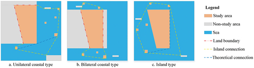
Herein, we propose a set of delimiting boundary lines known as the Offshore Island Connection Line (OICL) (Figure 1) and defined their delineation methods and principles for the first time. The Jinpu New Area in Dalian City, China, was selected as the study area. This area is bordered by the sea on both sides, has experienced rapid development, which is very suitable for research. Using the geographic simulation tool Geographic Simulation and Optimization System (GeoSOS) (Li et al. 2009a), we developed an artificial neural network (ANN) CA model from the perspective of the OICL (collectively, OICL-ANN-CA). We used the model to simulate the changes in the UDB in the study area, and compared the accuracy and spatial distribution of this model with those of the traditional perspective ANN-CA. Subsequently, land use change and landscape patterns for the study area in 2035 were predicted under three scenarios: historical inertia development (HID), ecological security protection (ESP), and ecological and economic balance (EEB).

Figure 1. Distribution types of the Offshore Island Connection Line (OICL).

This paper is organized as follows: the next section presents the literature review. Section 3 describes the concept and principles of the OICL and delineates the research boundary of the study area. Section 4 presents the research data and methods, and the validation and prediction results of the OICL-ANN-CA model are presented in Section 5. Finally, the last section summarizes the conclusions of the study and analyzes the contributions and limitations of the study, indicating future research directions.

2. Literature Review

2.1 The UDB concept

The term UDB comes from the western concept of the urban growth boundary, which is based on the theories of new urbanism and smart growth (Ding, Knaap, and Hopkins 1999; Nelson and Moore 1993). The UDB is the boundary between urban construction land and non-construction land, and it is a technical way and policy measure used to control the disorderly sprawl of the city. It was first used in Salem, Oregon, USA (Gustafson, Daniels, and Shirack 1982), and later became a control tool for urban development in the USA and many other countries worldwide (Harig et al. 2021; Tayyebi, Pijanowski, and Tayyebi 2011; Tayyebi, Perry, and Tayyebi 2013; Wang et al. 2020a) . The UDB is also the boundary line of the city's spatial expansion within a certain period and can be adjusted dynamically. The UDB has both rigid and flexible boundaries (Chakraborti et al. 2018; Chettry and Surawar 2021). The rigid boundary refers to the maximum construction scope that can be achieved under resource constraints. The flexible boundary refers to the range of urban construction land that meets the needs of economic and social construction within a certain period while ensuring the environment indicators. The UDB of this study is the concept of flexible boundary, which has the characteristics of dynamic aging and spatial elasticity. Another boundary is the research boundary, which refers to the geographical spatial distribution range of the research object. This boundary is typically based on administrative divisions (Yang et al. 2018), basins (Twisa and Buchroithner 2019), functional areas (Liu, Zhang, and Yang 2018) and land-sea boundaries (Chen, Zhang, and Jiang 2017), and so on. Generally, the boundary of the research scope is larger than that of the UDB.

2.2 Methods for delimiting UDBs

The methods for delimiting UDBs can be divided into three types: forward, reverse and comprehensive methods. First, the forward method regards urban construction land as a constantly changing organic whole, and comprehensively analyzes the development trend of the city based on factors such as the population, industry, resources, and transportation of the city. The cellular automata (CA) model is widely used in the simulation of urban expansion due to its discrete, bottom-up, parallel, and open characteristics (Li, Yang, and Liu 2008; Li et al. 2011a, 2012). The CA model is constantly being combined with new methods such as statistical analysis models, artificial intelligence optimization algorithms, system dynamics, multi-agents, and geographic partitions to obtain better simulation results (Azari et al. 2016; Geng, Zheng, and Fu 2017; Kong et al. 2017; Osman, Divigalpitiya, and Arima 2016; Xia and Zhang 2021; Yang et al. 2019). Although the forward method has high simulation accuracy, its bottom-up research mode ignores the top-down role of urban policy control, and the land management system and government macro-control and other external factors are less considered. Second, the reverse method delineates the ecological red line and basic farmland protection red line based on comprehensively considering the characteristics of the local natural environment. The least resistance model, ecological security pattern analysis, and land adaptability evaluation are typical reverse methods (Liu, Wei, and Zeng 2020; Sakieh et al. 2015; Wang et al. 2019). It is relatively easy to implement and can determine the maximum range of suitable urban construction. However, because the limiting factors are generally static and cannot reflect the internal driving mechanism of urban growth changes, it is difficult to understand the future development direction of the city. Third, the comprehensive method combines the forward and reverse methods. It first uses the reverse method to determine suitable construction areas and prohibited construction areas through suitability evaluation (Xu et al. 2018) or combining with planning policies that the government has formulated (Huang, Wang, and Xiao 2022). Afterward, the forward method is used to simulate the UDB based on factors such as the natural environment, population distribution, infrastructure, and CA elements (Feng and Tong 2018; Xia and Zhang 2021). The comprehensive method integrates the advantages of the previous methods, while organically unifying the natural resource background conditions and government's macro-control policies. However, there is also the problem of excessively complex conversion rules.

3 Offshore Island Connection Line

3.1 Definition and delimitation principles

The OICL is an established set of lines used to delimit the boundary of the study area, and consists of the largest outsourced lines of land or the main island and its affiliated islands. According to the sea–land boundary of the study area, when there is only one section of the offshore island connection as the land boundary, i.e. the study area is unilaterally coastal or peninsula region, this is defined as the unilateral coastal type (Figure 1). Similarly, when there are two land boundaries in the offshore island connection, i.e. the study area is on both sides of the sea, this is defined as the bilateral coastal type (Figure 1), and the Jinpu New Area belongs to this type. When there is no land boundary on the OICL and the study area is surrounded by sea (islands), defined as the island type (Figure 1).

To establish the reference standards in the actual delimitation process and outline the approach for certain special situations, we present the following four delimitation principles, defined for the first time. These principles can help relevant researchers delimit the OICL of their research area. The first is the full coverage principle, in which the closed range of the OICL should cover land and islands within the scope of all administrative divisions in the study area to ensure the integrity of the original territory (Figure 1). The second is the extension principle, in which there is an intersection between the island line and main boundary; thus, it is necessary to extend outward to the land or island vertex of the non-study area, thereby retaining a certain amount of sea space (Figure 1). This is to preserve a certain buffer zone. Theoretically, any sea area adjacent to land may be converted into urban land, ensuring that this part of the change can be simulated, which is also the core reason for the proposed OICL. The third is the exclusive principle, in which there is a non-study area within the scope of the connection, it is necessary to adjust the connection to the outer boundary of the non-research area to avoid including non-study areas (Figure 1). Any land not included in the study area would interfere with the simulation results. The fourth is the consistency principle, in which the land part of the line should be consistent with the land administrative boundary of the study area. There is no outward expansion in the land administrative boundary, and therefore, it should be strictly delimited according to the original boundary (Figure 1).

As a new way to delineate maritime boundaries, the OICL also needs to handle the relationship with existing boundaries such as the International Maritime Boundary Line (IMBL) (Stephen 2014). Because the OICL is a set of lines delineated based on the land or the main island and the islands under its jurisdiction, it includes both a land portion and sea area portion. The connecting part of the sea area typically extends to the outside of the island to which it belongs, which is similar to the Territorial Sea Baseline (TSB) (Specht et al. 2017). When there is no island or other land, it can also extend a certain distance outward based on the extension principle. In this case, we recommend that this distance should not exceed the territorial sea (12 nautical miles away from the TSB) to avoid unnecessary disputes.

If many islands lead to a complex drawing line, the initial boundary drawing can be directly completed using the ArcGIS10.6 minimum boundary geometry tool. Thus, a research boundary can be defined by editing and adjusting the lines according to the above principles.

3.2 Research boundary delineation of the study area

The Jinpu New Area occupies the central and southern parts of Dalian City in Liaoning Province, China, and is between 121°30ʹ07” E – 122°18ʹ46” E, 38°54ʹ49” N – 39° 32ʹ46” N (Figure 2). It is the tenth national new area (http://www.china.org.cn/business/2014-07/02/content_32838403.htm), with 25 streets in the Jinzhou District and three streets in the Pulandian District. The region experiences a temperate monsoon climatic, with marine climate characteristics. The terrain has a relatively high elevation in the middle and low elevation on both sides, with slight fluctuations. The Bohai Sea is shallower on the west side of the Jinpu New Area, whereas the Yellow Sea is deeper on the east side in the Jinpu New Area. At the end of 2020, the population was 1.545 million, the population density was 672 persons per km², and the gross domestic product was 232.04 billion yuan, which is approximately USD 36.44 billion.

Figure 2. Research boundary of the study area (the Jinpu New Area).

According to the principles of the OICL and the characteristics of the study area, the research boundary of the study area was delineated. Initially, based on the consistency principle, the northern and southern land boundaries of the study area were determined. Afterward, based on the full coverage principle, it was determined that the administrative boundary in the northern part of the new district enters the sea from the northern side of Xingshutun Street, and that the line passes through the outer side of Hei Islands, Dantuozi Islands, Sanliangmache Islands. Afterward, based on the extension principle, it was determined that the line passes through the northern vertex of the Xiaosanshan Islands and connects with the southern land boundary of the new area. Subsequently, based on the exclusive principle, the southern land boundary of the new district was connected to the northern side of the Dalian New Airport. Finally, based on the full coverage principle, the connecting line was connected from the northern side of the airport through the Shituozi Islands, and the Tu Islands were connected to the northern land boundary of the new area. Thus, the final research boundary of the study area was delimited based on the OICL (Figure 2). The newly defined region covers a total area of 2832.14 km².

4 Research data and methods

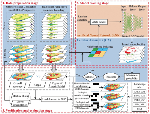
Figure 3 illustrates the three stages of developing the OICL-ANN-CA model. The first stage was the data preparation stage, in which the influencing factor data and land use data based on the OICL and traditional perspectives (sea–land boundary), were prepared, respectively. The second stage was the model training stage. In this stage, the input data were randomly sampled, and an ANN model was used to train and obtain the transfer probability of various types of land use by integrating the neighborhood effect. The third stage was the combination stage of verification and evaluation. After the threshold discrimination and use of the CA model, the simulation accuracies of the two perspectives were compared and analyzed using the overall accuracy, Kappa coefficient and figure of merit (FoM). Based on the land use data of historical years, combined with Markov chain and linear interpolation model, the urban construction land area of the study area in 2035 was calculated. The optimal perspective predicted the distribution of the UDB in the study area in 2035 and analyzed its landscape pattern.

Figure 3. Research framework.

4.1 Data source and processing

4.1.1 Data sources

The following types of data were utilized in this study: Landsat 5 Thematic Mapper (TM) imagery from 2000 and 2010, Landsat 8 Operational Land Imager (OLI) imagery from 2020, topographic elevation data from the Global Multi-Resolution Topography Synthesis (GMRT DEM) (Ryan et al. 2009), three types of space (urban space, agricultural space and ecological space), ecological red line delineation schemes, land use survey data, agricultural land and urban built-up areas, planning coastal reclamation areas data, coastline, road transport network and administrative division data. Table 1 shows the details of these data.

Table 1. Data source and description

Data type	Date of acquisition	Data	Resolution/scale	Sources
Raster data	17 September 2000	LANDSAT-5(TM)	30 m	Geospatial data cloud of computer network information center of Chinese Academy of Sciences (http://www.gscloud.cn)
	27 September 2010	LANDSAT-5(TM)
	20 June 2020	LANDSAT-8(OLI)
	2009	GMRT DEM	30 m/100 m	Global Multi-Resolution Topography Synthesis(https://www.gmrt.org/GMRTMapTool)
Vector data	2009, 2019	Land use survey data	1:10,000	Dalian Natural Resources Bureau
	2014	Three types of space (urban space, agricultural space and ecological space)	1:20,000	Dalian main functional area planning
		Ecological red line delimitation scheme
		Agricultural land
		Urban built-up areas
		Planning coastal reclamation areas
	2020	Coastline	1:50,000	Dalian administrative zoning map and Google Earth update
		Road transport network
		Administrative division

4.1.2 Land use data processing

The three phases of Landsat remote sensing images were preprocessed, including geometric corrections, radiometric corrections, cropping boundaries, supervised classification, visual interpretation, and boundary cleaning. These images were verified using the mastered land use survey data in 2009 and 2019, and the Kappa accuracy of the three images ranged from 0.81–0.86, meeting the requirements for almost perfect agreement with generally greater than 0.8 (Ozturk 2015; Zheng et al. 2015). Because the target study area is relatively large (2283.14 km²), higher resolution was expected to consume more computing resources and time. To reduce the hardware burden and shorten the calculation time, the original land use data were resampled under the premise of ensuring the simulation accuracy. These data were resampled to 100 × 100 m resolution to achieve the final land use status maps for the years 2000, 2010, and 2020 (Figure 4). The model was simulated with 2010 as the base year to highlight the differences in the simulation results caused by the delineation of the research boundaries. Hence, the three-period land use data from the traditional perspective were obtained by clipping the sea–land boundary in 2010, as shown in Figure 4. The four major land use categories identified were urban land, ecological forest land, cultivated land, and sea and land water body. Table 2 lists the specific land classification standards of the identified land use classes.

Figure 4. Land use classification in 2000, 2010, and 2020 under traditional and OICL perspectives (2010 coastline as reference boundary).

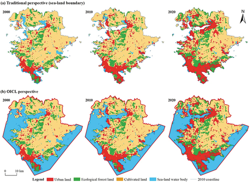
Table 2. Land use classification

Category	Describe
Urban land	Contains urban residential, industrial parks, urban facility land, forests (less than 1 km^2), excluding coastal salt fields, beaches
Ecological forest land	Forests (above or equal 1 km^2), orchard with ecological forest value
Cultivated land	Cultivated land, including facility agriculture, rural settlements, some orchards (new planting), etc.
Sea and land water body	Contains oceans, beaches, enclosures, land reservoirs, rivers

4.1.3 Treatment of influencing factors

Urban development is affected by natural and cultural factors. Eight factors were selected to reflect the potential of urban expansion. Referring to the relevant studies (Almeida et al. 2008; Gao et al. 2020; Ozturk 2015; Wang et al. 2016; Yang et al. 2019), they can be divided into three types: natural environment, infrastructure, and planning constraints (Table 3) and can be described as follows. First, natural environment factors, among which altitude and slope are widely used as influencing factors (Chen et al. 2020; Feng and Tong 2019; Huang et al. 2014; Xu et al. 2021), are the basis for urban development. The study area is located in the hilly area of Liaodong Peninsula. Both sides are coastal areas, and the terrain is undulating. The terrain conditions greatly affect the layout of the city. The coastal zone has good environmental and fishery resources, is suitable for human habitation. Herein, the distance to coastline should be used as an important factor in the model building (Guo, Zhang, and Hao 2020; Yang et al. 2014). Altitude and slope were obtained from the GMRT DEM data, and the distance to coastline was obtained by buffer analysis. Second, infrastructure, in which the urban built-up areas have perfect facilities to provide people with production and living, and its edge are easy to transform into an expansion area for new urban land (Liang et al. 2018; Liu et al. 2016). The traffic network carries the flow of people and goods, which can meet the needs of people's travel and goods trading. Surrounding residents tend to gather along the road, especially the intersections, so these places usually have a higher urban transformation potential (Van Berkel et al. 2019). The distance to urban built-up areas and the distance to expressways and trunk roads were obtained via buffer analysis. Third, planning restrictions, which are affected by food security and environmental protection policies, ecological red lines, basic farmland and land water (which has been integrated into the distance to coastline factor) in land use (Zhou et al. 2020), are limiting factors for urban development as these land types are rarely allowed to be converted to urban land. As the core achievement of land space planning, the preliminary division scheme of three types of space guide the direction of future urban development. The distance to ecological red line was obtained by performing a buffer analysis of the protected area, and the land use and the preliminary division scheme of three types of space were obtained by setting probabilities using a raster calculator according to the layer properties. To eliminate the dimensional differences and reduce the calculation amounts, the above layers were treated as standardized layers with intervals of [0, 1] and grid units of 100 × 100 m (Figure 5). Similarly, the layers of influencing factor from the traditional perspective were obtained by clipping the sea–land boundary (Figure 5). The basic descriptive statistics of all eight factors computed from the OICL and traditional boundary are shown in Figure 6.

Figure 5. Spatial distribution of eight influencing factors under traditional and OICL perspectives (see Table 3 for the meanings of the labels and units).

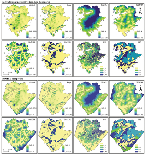
Figure 6. Boxplots of eight influencing factors under traditional and OICL perspectives (see Table 3 for the meaning of the labels).

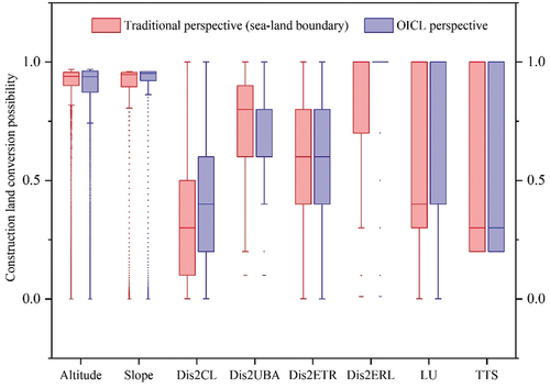
Table 3. Description of influencing factors

Type	Labels	Influence factor	Treatment method and description	Probability change curve
Naturalenvironment	Altitude	Altitude	ArcGIS raster to point tool and excel logistic regression method, raster data is processed into point set. The greater the altitude (H), the less likely it is to be selected as construction land . Collect and sort 21 samples corresponding to the construction land conversion possibility and altitude (see supplementary materials), and fit the following exponential equation:${\mathrm{P}}_{\mathrm{u}\mathrm{r}\mathrm{b}\mathrm{a}\mathrm{n}\mathrm{\_}\mathrm{H}}=1/\left(1+{\mathrm{e}}^{-\left(3.4255-0.0177\mathrm{H}\right)}\right)$Using this equation, the conversion probability of construction land at any altitude is calculated.
	Slope	Slope	ArcGIS raster to point tool and excel logistic regression method, raster data is processed into point set. The greater the slope (S), the less likely it is to be selected as construction land (${\mathrm{P}}_{\mathrm{u}\mathrm{r}\mathrm{b}\mathrm{a}\mathrm{n}\mathrm{\_}\mathrm{S}}$). Collect and sort 21 samples corresponding to the construction land conversion possibility and slope (see supplementary materials), and fit the following exponential equation:${\mathrm{P}}_{\mathrm{u}\mathrm{r}\mathrm{b}\mathrm{a}\mathrm{n}\mathrm{\_}\mathrm{S}}=1/\left(1+{\mathrm{e}}^{-\left(3.1804-0.1035\mathrm{S}\right)}\right)$Using this equation, the conversion probability of construction land at any slope is calculated.
	Dis2CL	Distance to coastline	ArcGIS multi-loop buffer analysis, within 1 km on both sides of the coastline, the conversion probability is set to 0.6, each outward expansion of 2 km, the conversion probability decreases 0.1, from the coastline 9–17 km probability is 0.1. Planning reclamation areas completely open conversion, set to 1, beach water part can be converted, set to 0.65, land water is not allowed to occupy, set to 0.001.
Infrastructure	Dis2UBA	Distance to urban built-up areas	ArcGIS multi-loop buffer analysis, within 1 km outside the urban built-up areas, the conversion probability is set to 0.8, each outward expansion of 2 km, the conversion probability decreased 0.2, from the edge of the urban built-up areas 7–11 km probability is 0.1. The probability of existing urban built-up areas is 1, and the infrastructure coverage area is 0.9.
	Dis2ETR	Distance to expressways and trunk roads	ArcGIS multi-loop buffer analysis, the probability within the range of 0.2 km from high speed and main road is set to be 1, 0.8 within 0.2–0.5 km, 0.6 within 0.5–1 km, 0.4 within 1–2 km, 0.2 within 2–3 km, 0.1 within 3–4 km, 0.01 within 4–5 km, 0.001 within 5–6 km, and 0.
Planning restrictions	Dis2ERL	Distance to ecological red line	ArcGIS multi-loop buffer analysis, the probability of 100 meters outside the ecological red line is 0.01, 0.1 within 100–200 meters, each outward expansion of 100 meters, the conversion probability increases by 0.2, the probability of 500 meters away from the ecological red line is 1, and the ecological red line area is set to 0.
	LU	Land use	ArcGIS grid calculator, other land types completely open conversion, general garden, woodland, cultivated land permit conversion, basic farmland in principle does not permit conversion, set other land 1, garden 0.7, woodland 0.4, cultivated land 0.3, basic farmland 0.001.	– –
	TTS	Preliminary division scheme of three types of space	ArcGIS grid calculator, unchanged urban space, low conversion of agricultural space, strict control of ecological space, land urban space 1, sea urban space 0.8, land and sea agricultural space 0.3, land and sea ecological space 0.2.	– –

4.2 Research methods

4.2.1 Simulation and prediction of the urban development boundary

The GeoSOS was proposed by Professor Xia Li, and developed by his team based on CA, multi-agent modeling, and spatial optimization (Li et al. 2009b). GeoSOS is an integrated model for data editing and basic analysis. The model displays support functions of a geographic information system platform and has simulation and optimization functions for geographic simulation tools, representing a set of theories, methods, and tools. This is important for studying complex geographic pattern changes (Li et al. 2009a). GeoSOS has been applied in many practical cases such as in urban simulation and spatial optimization (Li et al. 2011b), planning path optimization (Li et al. 2011c), protected area zoning (Li et al. 2011a), geographical condition analysis (Li, Li, and Liu 2017a), land use change (Chen et al. 2010), UDB expansion (Ma and Li 2019), and environment evolution (Wang et al. 2020b). In this study, we utilized the ANN-CA model component in GeoSOS.

The calculation of the cell transition probability is the most critical and complex part of the multi-type land use change problem. Previous studies required considerable time and calculations to compute the cell transition probability (Clarke and Gaydos 1998). Li and Yeh (2002) developed a fast, convenient, and automatic method for obtaining the transition rules and generating the transition probability of each cell by introducing an ANN to the CA model. The ANN-CA model comprises an input layer, hidden layer, and output layer. The input layer injects the cell attribute values and influencing factors into the hidden layer, and the output layer generates the final transition probability from the hidden layer to the response value. The calculation formula of the cell transition probability with random factor as follows:

(1) $p(k,t,l)=(1+(-1ny{)}^a)\times p_{ann}(k,t,l)\times {\mathrm{\Omega }}_k^t\times con(s_k^t)$(1)

In the formula, denotes the overall conversion probability of type land in cell $\hspace{0.17em}k$ and time $\hspace{0.17em}k$, $1+\hspace{0.17em}\left(-lny\right)$ is a random number, $P_{ann}(k,t,l$ denotes the transition probability of $l$ type land in cell $k$ and time $1+\hspace{0.17em}\left(-lny\right)$ trained by the ANN method, ${\mathrm{\Omega }}_k^t$ denotes the proportion of urban land in the neighborhood window, and $con\left(S_k^t\right)$ represents the suitability of conversion between the two land use types, with a value ranging from 1 or 0, which can either be transferred or not transferred.

4.2.2 Verification and evaluation of simulation accuracy

The accuracy of the land use simulation is the key criterion for land use change prediction, and its value directly affects the final results. At present, the user accuracy, producer accuracy, overall accuracy (Olofsson et al. 2014), Kappa coefficient (Stehman 1997), FoM (Pontius et al. 2008), and other parameters are typically used. Therefore, in this study, the accuracy of the simulation results was verified based on the above parameters. Among them, the Kappa coefficient was considered as the most representative and comprehensive metric for computing accuracy and, is mathematically expressed as follows:

(2) $k=\frac{p_0-p_e}{1-p_e}$(2)

where $p_0$ represents the proportion of correctly classified samples, and $p_e$ represents the proportion of the sum of the product of the total number of actual samples and total number of predicted samples to the square of the total number of samples. Generally, a Kappa coefficient above 0.6 indicates an simulation effect indicating “substantial agreement,” and a value greater than 0.8 indicates an “almost perfect agreement” of the simulation effect (Tong and Feng 2020).

The FoM only evaluates the accuracy of changing pixel simulation, not the statistics of all pixels; therefore, it better reflects the simulation results. The FoM is expressed as follows:

(3) $FoM=B/(A+B+C+D)$(3)

where A is the error region of actual change but unchanged simulation, B is the correct region of actual change and consistent prediction category, C is the error region of actual change but inconsistent prediction category, and D is the error region of actual change but unchanged simulation.

The above indicators can be used to evaluate the simulation effect at the macro-level, however, the landscape index is more conducive to finding differences between the various patches in the land use pattern and showing information at the micro-level (McGarigal and Marks 1995). To reduce redundancy between the indicators and to meet our research needs, the core indicators proposed by Tian and others (2019) were selected, including AREA_AM (patch area_ area-weighted mean, reflecting the average patch area), FRAC_AM (fractal dimension index_ area-weighted mean, reflecting the shape complexity), PARA_CV (perimeter-area ratio_ coefficient of variation, reflecting the shape complexity variation), ENN_AM (Euclidean nearest neighbor distance_ area weighted average, reflecting the spatial dispersion), and TECI (total edge contrast index, reflecting the landscape fragmentation). Fragstats4.2 was used to calculate the results.

5 Results

5.1 Model and its precision

Based on the traditional and OICL perspectives, the supervised classification results of the years 2000 and 2010 were used as rules to extract the land use data layer of the initial year and end year, and the eight influencing factor layers under the corresponding perspective were used as inputs. The ANN-CA method was used considering a 5% proportional sampling and set as the total change according to the newly added urban land area of 194.08 km² from 2010 to 2020. Urban land could not be converted to other land types; however, the remaining land types could be converted to other land types. Two hundred iterations were set, the diffusion coefficient was 1, and the conversion threshold was 0.9. For comparison with real classification results in 2020, the simulation results from the traditional perspective (sea–land boundary) in 2020 supplemented the missing sea area according to the sea-land boundary in 2020. Finally, the land use results of 2020 under the two perspectives were simulated and compared with the real classification for 2020 (Figure 7).

Figure 7. Real and simulated land use under traditional and OICL perspectives in 2020.

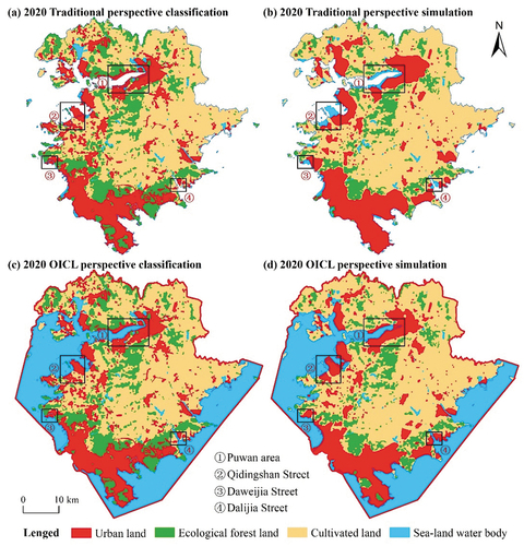
The classification accuracy was calculated using point-to-point verification of the simulation results obtained in 2020 and land classification results from the two perspectives (Table 4). According to the accuracy evaluation index, the OICL perspective was better than the traditional perspective (sea–land boundary). The overall accuracies of the OICL and traditional perspectives (sea–land boundary) were 83.57% and 75.42%, respectively, indicating that the OICL perspective was improved by 8.15%, whereas the Kappa coefficients were 0.768 and 0.601, respectively. Both perspectives fell into the “qualified” category, and the OICL perspective was better by 0.167 (approximately 27.79%). The FoM, which only reflects the accuracy of change cell simulation, was 0.172 and 0.128 for the OICL and traditional perspectives (sea–land boundary), respectively, with the OICL perspective showing a value 34.38% higher than that of the traditional perspective. Based on the land layout of the simulation results, the traditional perspective (sea–land boundary) was limited by the research boundary; hence, coastal reclamation areas could not be effectively simulated, and some ecological forest land was occupied. The OICL perspective of the sea–land combination effectively simulated sea area expansion of the UDB, particularly in the Puwan area (Figure 7, [1]) and for Qidingshan Street (Figure 7, [2]), Daweijia Street (Figure 7, [3]), and Dalijia Street (Figure 7, [4]), as well as other locations. The conversion of ecological forest land to urban land was relatively small, which protects ecological forest land from excessive destruction. We compared the results from this study with those of two similar studies (Huang, Huang, and Liu 2019; Xu, Gao, and Coco 2019). Although the simulation accuracy of the OICL perspective met only the basic requirements (0.6 < kappa ≤ 0.8, substantial agreement), the simulation achieved very good simulation results for urban land expansion in some sea areas, demonstrating the scientific nature of the model construction and necessity of using the OICL perspective for land use change prediction in coastal areas.

Table 4. Classification accuracy evaluation

Perspective	Overall accuracy	Kappa	FoM
Traditional perspective (sea–land boundary)	75.42%	0.601	0.128
OICL perspective	83.57%	0.768	0.172

5.2 Scenario simulation and parameter set-up

To reflect the development differences of different paths, three scenarios were set up: the HID scenario, the ESP scenario, and the EEB scenario. The HID scenario is a baseline scenario that did not consider any other interference factors but was still in accordance with the past development path. In this scenario, urban land could not be converted to other land types, whereas remaining land types could be freely converted to completely open coastal reclamation areas. The ESP scenario emphasizes ecological security issues, implemented the most stringent protection system, prohibited any ecological forest land and sea–land water encroachment, and completely limited coastal reclamation behavior. The EEB scenario focuses on ecological protection and simultaneously considered economic and social development and limited the occupation of ecological forest land by construction land, while allowing some coastal reclamation behaviors based on construction needs. The specific rules for the land conversion matrix are shown in Figure 8.

Figure 8. Setting of the land use conversion matrix for HID, ESP, and EEB scenarios.

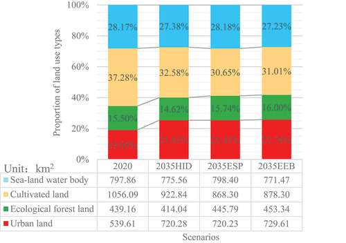
As a random process research method, the core idea of the Markov chain is that the future state is only related to the current state, which is very similar to the change form of land use (Ching and Mooney 1971). The Markov chain has been widely used to predict future land total use in similar studies (Bai et al. 2018; Liang et al. 2021). In the prediction stage, the urban construction land area in 2030 and 2040 was calculated based on Markov chain. Combined with historical data, the linear interpolation method was used to obtain a prediction of the urban construction land area of the study area in 2035, which is 730.24 km², and a prediction of the total area demand for urban construction land in the next 15 years, which is approximately 190 km². To ensure the stability of each scenario, the random sampling rate was increased to 20%, and the other parameter settings were the same as those used at the accuracy verification stage.

5.3 Land use pattern in 2035

Expecting an increase in the demand for the UDB in the future, the land use distributions under the three scenarios (HID, ESP, and EEB) in the study area in 2035 were predicted based on the results of the land use classification in 2020 (Figure 9). The results showed that the land use pattern of the new district will undergo profound changes in the future. Macroscopically, urban land use under the three scenarios indicated that the Jinzhou and Puwan areas were the core expansion areas, with Qidingshan, Taiping, and Fuzhouwan streets along the Yellow Sea coast and Desheng, Dalijia, and Dengshahe streets along the Bohai Sea coast as several additional important clusters of urban growth. Overall, the land use patterns were similar between different scenarios. To analyze the differences between the core expansion areas and scenarios of future urban land expansion in the new area, the prediction results of each scenario were superimposed with the land use data in 2020, and a type composition distribution map of the new urban land was obtained (Figure 9). Figure 8 shows some of the key areas of change in the amplified maps. In all three scenarios, the most evident urban land expansion occurred in the (1) Songmudao, (2) Puwan, and (5) Desheng Street areas (Figure 9). This may be because these areas are consistent with the areas impacted by industrial and regional development policies, such as the Songmudao Chemical Industrial Park (National Circular Economy Demonstration Park), Dalian (Puwan) Administrative Center, and Advanced Equipment Manufacturing Industrial Park, built on Desheng Street.

Figure 9. The 2035 land use patterns and the composition of new urban land under HID, ESP, and EEB scenarios.

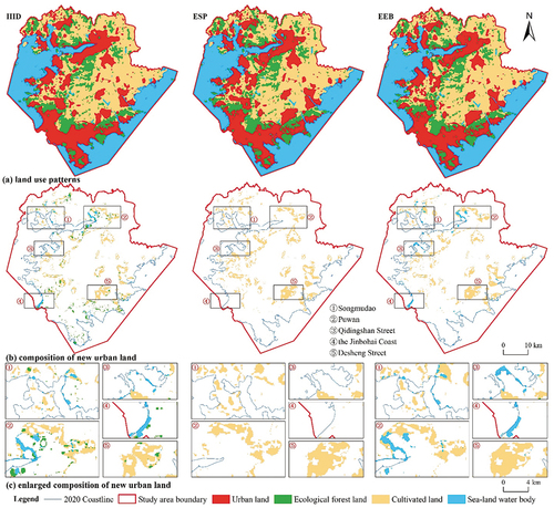
In all scenarios, it was necessary to consider the protection of ecological corridors and maintain the ecological security pattern of (one ridge and multi-corridor, connected mountains and seas) within Dalian City (https://zrzy.dl.gov.cn/art/2020/4/20/art_3083_506764.html). In the HID scenario, in addition to farmland, some ecological forest land was transformed to urban land and was primarily distributed on the northern side of the Jinzhou area and southern side of the Puwan area. In the (1) Songmudao, (2) Puwan, and (5) Desheng Street areas (Figure 9), some inland waters were converted to urban land in both the HID and EEB scenarios, whereas forest land and water in the ESP scenario were not converted and were well protected. In addition, under the EEB and HID scenarios, there were portions of sea converted into urban land in the areas near (3) Qidingshan Street and (4) the Jinbohai Coast (Figure 9), indicating the future possibility of urban expansion into the sea. As the Qidingshan coast area is a new Japanese industrial group area of the China–Japan (Dalian) Local Development Demonstration Area, and the Jinbohai Coast is a key support area of the Liaoning Coastal Economic Belt construction and is adjacent to Dalian New Airport, there will be a large number of urban land development and construction needs that may be affected by relevant policies and their strategic locations. Under the ESP scenario, no change in land and sea was affected by the simulation policy.

To further evaluate the distribution characteristics and differences in each scenario and provide more reference information for planners and decision makers in the delineation of the UDB, the landscape pattern indices of each scenario were compared (Table 5). The AREA_AM indices of each land use type significantly differed under the three scenarios. In terms of urban land use, the AREA_AM index of the HID scenario was highest, indicating that land use was relatively concentrated, and the patch area was largest, followed by that in the ESP scenario. Because of the restrictions to land conversion, except for cultivated land, urban land use was mostly limited to extended development of the cultivated land concentrated areas. In fact, the EEB scenario hindered the generation of large urban patches because of the barrier effect of ecological land use and conversion to sea–land water bodies. Thus, the AREA_AM index value was lowest in all scenarios. Overall, the FRAC_AM and PARA_CV indices reflected the complexity and difference of the patch shapes. These two indices for urban land were highest in the ESP scenario, whereas those for cultivated land were lowest, indicating that a large amount of urban land expanded to the cultivated land, and the cultivated land boundary became smoother. However, urban land adjacent to the sea–land water body and ecological forest land maintained the original boundary, which was complex and changeable. In contrast, the complexity of the patch shape within a single land category was quite different. The urban land boundary in the HID scenario was the smoothest, and the internal difference was the smallest. The FRAC_AM and PARA_CV indices of the EEB scenario were between those of the ESP and HID scenarios. The ENN_AM index reflects the degree of dispersion of the same land type. With respect to this index, the urban land under the HID scenario was relatively dispersed, and the independence between urban patches was strong. The distribution of urban land under the EEB scenario was relatively concentrated, and urban patches exhibited good connectivity. The connectivity of the ESP scenario was between those of the two other scenarios.

Table 5. Comparison of landscape pattern index of each scenario

Scenario	Type	AREA_AM	FRAC_AM	PARA_CV	ENN_AM	TECI
HID	Urban land	14,508.49	1.14	78.65	354.56	65.54
	Ecological forest land	1901.54	1.12	67.57	358.65	83.63
	Cultivated land	71,524.06	1.23	47.65	213.24	73.44
	Sea-land water body	37,044.12	1.15	50.36	213.15	68.67
ESP	Urban land	12,919.88	1.16	80.11	315.48	68.96
	Ecological forest land	1934.21	1.12	57.51	320.28	82.42
	Cultivated land	64,318.13	1.22	45.92	212.38	74.51
	Sea-land water body	38,197.32	1.16	47.05	211.01	70.54
EEB	Urban land	11,916.54	1.15	79.14	303.21	68.14
	Ecological forest land	2576.13	1.13	58.53	310.38	82.13
	Cultivated land	65,679.15	1.23	47.00	223.71	74.38
	Sea-land water body	36,946.11	1.15	49.06	211.15	68.74

6 Discussion and conclusions

We constructed the OICL-ANN-CA model based on the perspective of the OICL. This model was used to simulate land use change in the Jinpu New Area of Dalian City, China, from 2000 to 2020. We developed multi-scenario projections for land use patterns in 2035, and analyzed differences in these patterns among the scenarios. In contrast to the concepts proposed in previous studies to improve the accuracy of data (Bai et al. 2018; Li et al. 2017b) and algorithms (Omrani, Tayyebi, and Pijanowski 2017; Zhou et al. 2020), we focused on the influence of the research boundary delineation on land use simulation results in rapidly urbanizing coastal areas. We verified the effectiveness of the OICL-ANN-CA model for urban land expansion simulation. The results showed that the overall accuracy, Kappa coefficient, and FoM in the model validation stage from the OICL perspective were 83.57%, 0.768, and 0.172, respectively. Compared with those of the traditional perspective, these values increased by 8.15%, 27.79%, and 34.38%, respectively. Notably, we set the coastline as the research boundary for the traditional perspective. Consequently, the conversion of sea to construction land was missing in these simulations. Even if the administrative divisions were used as the research boundary, along with the influence of rapid development of the city, there was some construction land outside the boundary that could not be simulated. However, this situation can be effectively avoided based on the OICL perspective. In addition, the significant improvement in the key indicator, FoM (Li et al. 2021; Zhang and Wang 2021), highlights the capability of the OICL-ANN-CA model for UDB simulation.

We predicted future trends for the UDB in the Jinpu New Area under multiple scenarios (Figures 9, 10), and realized an effective simulation of potential land for urban construction outside the traditional boundary. The ESP scenario was subject to strict control policies, with no reclamation. However, in the HID and EEB scenarios, there were some conversions from coastal water bodies to urban land. Compared with the large number of coastal reclamation areas that have appeared in the past 20 years, the scale of conversion in the future will be smaller, and mostly distributed in key construction areas. The results of the above multi-scenario prediction show that the OICL-ANN-CA model conforms to current marine protection and development policies and can capture the subtleties of coastal reclamation construction within the region, particularly in the EEB scenario. The growth of urban land outside the traditional boundary described in the HID and EEB scenarios was also noted by Liang and others (2018). They used the Clustering-based Future Land Use Simulation (CFLUS) model to find potential urban development land in the sea area without any original urban area. The CFLUS model can provide decision support for the establishment of development zones. Whether the isolated growth of urban land detected in the ocean by Liang and others (2018), or the fringe growth of urban land found outside the traditional boundary in this study, the findings of these two types of urban land growth illustrate the importance of using a similar OICL perspective to expand the research boundary in coastal city land use simulation studies.

Figure 10. Area and proportion of land use types in 2020 and three scenarios of 2035.

Furthermore, unlike methods that delimit the research scope according to isobath or marine functional zoning data, functional zoning at different administrative levels is difficult to determine because of factors such as data confidentiality and incomplete data for planning processes. However, the OICL required no external data. Thus, the study area at any administrative level could be quickly framed, ensuring the stability of the study area to ensure convenience and flexibility in delimiting the research boundary.

This study, demonstrates that the OICL-ANN-CA model can effectively detect the growth of new urban land outside the traditional boundary that was neglected in the past, and improve the accuracy of UDB simulation. This study has the following limitations. Political and economic conditions are increasingly dominant factors that influence urban development (Li et al. 2018; Yang et al. 2021). Data regarding the population of the study area, night lighting, points of interest, and coastal zone protection policies could be added to further improve the simulation results. In the future, the sensitivity of different factors influencing the simulation results and optimal regulation path analysis of the UDB are also worth exploring. Moreover, the model could be compared with other excellent modeling methods and applied to more regions to further validate this method.

Data availability

Data are available on request.

Acknowledgements

The authors would like to acknowledge all colleagues and friends who have voluntarily reviewed the translation of the survey and the manuscript of this study.

Disclosure statement

No potential conflict of interest was reported by the author(s).

Supplementary material

Supplemental data for this article can be accessed online at https://doi.org/10.1080/15481603.2022.2071056

Correction Statement

This article has been republished with minor changes. These changes do not impact the academic content of the article.

Additional information

Funding

This research study was supported by the National Natural Science Foundation of China (grant nos. 41771178, 42030409, 41671151), the Fundamental Research Funds for the Central Universities (grant no. N2111003), the Second Tibetan Plateau Scientific Expedition and Research Program (STEP) (grant no. 2019QZKK1004), and the Innovative Talents Support Program of Liaoning Province (grant no. LR2017017).

References

- Almeida, C. M., J. M. Gleriani, E. F. Castejon, and B. S. Soares-Filho. 2008. “Using Neural Networks and Cellular Automata for Modelling Intra-urban Land-use Dynamics.” International Journal of Geographical Information Science 22 (9): 943–963. doi:10.1080/13658810701731168.
- Azari, M., A. Tayyebi, M. Helbich, and M. A. Reveshty. 2016. “Integrating Cellular Automata, Artificial Neural Network, and Fuzzy Set Theory to Simulate Threatened Orchards: Application to Maragheh, Iran.” GIScience and Remote Sensing 53 (2): 183–205. doi:10.1080/15481603.2015.1137111.
- Bai, X., P. Shi, and Y. Liu. 2014. “Society: Realizing China’s Urban Dream.” Nature 509 (7499): 158–160. doi:10.1038/509158a.
- Bai, Y., C. P. Wong, B. Jiang, A. C. Hughes, M. Wang, and Q. Wang. 2018. “Developing China’s Ecological Redline Policy Using Ecosystem Services Assessments for Land Use Planning.” Nature Communications 9 (1): 1. doi:10.1038/s41467-018-05306-1.
- Chakraborti, S., D. N. Das, B. Mondal, H. Shafizadeh-Moghadam, and Y. Feng. 2018. “A Neural Network and Landscape Metrics to Propose A Llexible Urban Growth Boundary: A Case Study.” Ecological Indicators 93: 952–965. doi:10.1016/j.ecolind.2018.05.036.
- Chen, S., Y. Feng, Z. Ye, X. Tong, R. Wang, S. Zhai, C. Gao, Z. Lei, and Y. Jin. 2020. “A Cellular Automata Approach of Urban Sprawl Simulation with Bayesian Spatially-varying Transformation Rules.” GIScience and Remote Sensing 57 (7): 924–942. doi:10.1080/15481603.2020.1829376.
- Chen, Y., X. Li, X. Liu, and S. Li. 2010. “Coupling Geosimulation and Optimization (Geosos) for Zoning and Alerting of Agricultural Conservation Areas.” Acta Geographica Sinica 65 (9): 1137–1145. doi:10.11821/xb201009011.
- Chen, B., Y. Zhang, and D. Jiang. 2017. “Urban Land Expansion in Fuzhou City Based on Coupled Cellular Automata and Agent-based Models (CA-ABM).” Progress in Geography 36 (5): 626–634. doi:10.18306/dlkxjz.2017.05.010.
- Chettry, V., and M. Surawar. 2021. “Delineating Urban Growth Boundary Using Remote Sensing, ANN-MLP and CA Model: A Case Study of Thiruvananthapuram Urban Agglomeration, India.” Journal of the Indian Society of Remote Sensing 49 (10): 2437–2450. doi:10.1007/s12524-021-01401-x.
- Ching, C. T. K., and M. B. Mooney. 1971. “Land Use Protection through Air Photos and Markov Chain.” Proceedings, Annual Meeting (Western Agricultural Economics Association) 44: 131–133.
- Clarke, K. C., and L. J. Gaydos. 1998. “Loose-coupling a Cellular Automaton Model and GIS: Long-term Urban Growth Prediction for San Francisco and Washington/Baltimore.” International Journal of Geographical Information Science 12 (7): 699–714. doi:10.1080/136588198241617.
- Ding, C., G. J. Knaap, and L. D. Hopkins. 1999. “Managing Urban Growth with Urban Growth Boundaries: A Theoretical Analysis.” Journal of Urban Economics 46 (1): 53–68. doi:10.1006/juec.1998.2111.
- Feng, Y., and X. Tong. 2018. “Dynamic Land Use Change Simulation Using Cellular Automata with Spatially Nonstationary Transition Rules.” GIScience and Remote Sensing 55 (5): 678–698. doi:10.1080/15481603.2018.1426262.
- Feng, Y., and X. Tong. 2019. “Incorporation of Spatial Heterogeneity-weighted Neighborhood into Cellular Automata for Dynamic Urban Growth Simulation.” GIScience and Remote Sensing 56 (7): 1024–1045. doi:10.1080/15481603.2019.1603187.
- Gao, C., Y. Feng, X. Tong, Z. Lei, S. Chen, and S. Zhai. 2020. “Modeling Urban Growth Using Spatially Heterogeneous Cellular Automata Models: Comparison of Spatial Lag, Spatial Error and GWR.” Computers, Environment and Urban Systems 81: 101459. doi:10.1016/j.compenvurbsys.2020.101459.
- Geng, B., X. Zheng, and M. Fu. 2017. “Scenario Analysis of Sustainable Intensive Land Use Based on SD Model.” Sustainable Cities and Society 29: 193–202. doi:10.1016/j.scs.2016.12.013.
- Guo, A., Y. Zhang, and Q. Hao. 2020. “Monitoring and Simulation of Dynamic Spatiotemporal Land Use/Cover Changes.” Complexity 2020: 1–12. doi:10.1155/2020/3547323.
- Gustafson, G. C., T. L. Daniels, and R. P. Shirack. 1982. “The Oregon Land Use Act Implications for Farmland and Open Space Protection.“ Journal of the American Planning Association 48 (3): 365–373. doi:10.1080/01944368208976185.
- Harig, O., R. Hecht, D. Burghardt, and G. Meinel. 2021. “Automatic Delineation of Urban Growth Boundaries Based on Topographic Data Using Germany as a Case Study.” ISPRS International Journal of Geo-Information 10 (5): 353. doi:10.3390/ijgi10050353.
- Huang, Q., C. He, Z. Liu, and P. Shi. 2014. “Modeling the Impacts of Drying Trend Scenarios on Land Systems in Northern China Using an Integrated SD and CA Model.” Science China Earth Sciences 57 (4): 839–854. doi:10.1007/s11430-013-4799-7.
- Huang, D., J. Huang, and T. Liu. 2019. “Delimiting Urban Growth Boundaries Using the CLUE-S Model with Village Administrative Boundaries.” Land Use Policy 82: 422–435. doi:10.1016/j.landusepol.2018.12.028.
- Huang, M., C. Kou, and W. Qu. 2012. “Combining Rigidity and Flexibility: Reflection on Urban Growth Boundary.” Planners 28 (3): 12–15. doi:10.3969/j.issn.1006-0022.2012.03.002.
- Huang, X., H. Wang, and F. Xiao. 2022. “Simulating Urban Growth Affected by National and Regional Land Use Policies: Case Study from Wuhan, China.” Land Use Policy 112: 105850. doi:10.1016/j.landusepol.2021.105850.
- Kong, L., G. Tian, B. Ma, and X. Liu. 2017. “Embedding Ecological Sensitivity Analysis and New Satellite Town Construction in an Agent-based Model to Simulate Urban Expansion in the Beijing Metropolitan Region, China.” Ecological Indicators 82: 233–249. doi:10.1016/j.ecolind.2017.07.009.
- Li, X., Y. Chen, X. Liu, D. Li, and J. He. 2011b. “Concepts, Methodologies, and Tools of an Integrated Geographical Simulation and Optimization System.” International Journal of Geographical Information Science 25 (4): 633–655. doi:10.1080/13658816.2010.496370.
- Li, X., G. Chen, X. Liu, X. Liang, S. Wang, Y. Chen, F. Pei, and X. Xu. 2017b. “A New Global Land-Use and Land-Cover Change Product at A 1-km Resolution for 2010 to 2100 Based on Human–Environment Interactions.” Annals of the American Association of Geographers 107 (5): 1040–1059. doi:10.1080/24694452.2017.1303357.
- Li, X., C. Lao, X. Liu, and Y. Chen. 2011a. “Coupling Urban Cellular Automata with Ant Colony Optimization for Zoning Protected Natural Areas under a Changing Landscape.” International Journal of Geographical Information Science 25 (4): 575–593. doi:10.1080/13658816.2010.481262.
- Li, X., D. Li, and X. Liu. 2017a. “Geographical Simulation and Optimization System (Geosos) and Its Application in the Analysis of Geographic National Conditions.” Acta Geodaetica et Cartographica Sinica 46 (10): 1598–1608. doi:10.11947/j.AGCS.2017.20170355.
- Li, X., D. Li, X. P. Liu, and J. He. 2009b. “Geographical Simulation and Optimization System (Geosos) and Its Cutting-edge Researches.” Advances in Earth Science 24 (8): 899–907. doi:10.3321/j.issn:1001-8166.2009.08.007.
- Li, X., J. Lin, J. Chu, and Y. Zhao. 2020. “Research on Land-ocean Planning Method in Territorial Space Planning.” China Land Science 34 (5): 60–68. doi:10.11994/zgtdkx.20200420.095652.
- Li, X., X. Liu, J. He, D. Li, Y. Chen, Y. Pang, and S. Li. 2009a. “A Geographical Simulation and Optimization System Based on Coupling Strategies.” Acta Geographica Sinica 64 (8): 1009–1018. doi:10.11821/xb200908012.
- Li, J., Y. Liu, Y. Yang, and J. Liu. 2018. “Spatial-temporal Characteristics and Driving Factors of Urban Construction Land in Beijing-Tianjin-Hebei Region during 1985-2015.” Geographical Research 37 (1): 37–52. doi:10.11821/dlyj201801003.
- Li, X., X. Shi, J. He, and X. Liu. 2011c. “Coupling Simulation and Optimization to Solve Planning Problems in a Fast-Developing Area.” Annals of the Association of American Geographers 101 (5): 1032–1048. doi:10.1080/00045608.2011.577366.
- Li, X., Q. Yang, and X. Liu. 2008. “Discovering and Evaluating Urban Signatures for Simulating Compact Development Using Cellular Automata.” Landscape and Urban Planning 86 (2): 177–186. doi:10.1016/j.landurbplan.2008.02.005.
- Li, X., and A. G. Yeh. 2002. “Neural-network-based Cellular Automata for Simulating Multiple Land Use Changes Using GIS.” International Journal of Geographical Information Science 16 (4): 323–343. doi:10.1080/13658810210137004.
- Li, X., J. Zhang, Z. Li, T. Hu, Q. Wu, J. Yang, J. Huang, et al. 2021. “Critical Role of Temporal Contexts in Evaluating Urban Cellular Automata Models.” GIScience and Remote Sensing 58 (6): 799–811. doi:10.1080/15481603.2021.1946261.
- Li, X., Y. Zhang, X. Liu, and Y. Chen. 2012. “Assimilating Process Context Information of Cellular Automata into Change Detection for Monitoring Land Use Changes.” International Journal of Geographical Information Science 26 (9): 1667–1687. doi:10.1080/13658816.2011.643803.
- Liang, X., Q. Guan, K. C. Clarke, S. Liu, B. Wang, and Y. Yao. 2021. “Understanding the Drivers of Sustainable Land Expansion Using A Patch-generating Land Use Simulation (PLUS) Model: A Case Study in Wuhan, China.” Computers, Environment and Urban Systems 85: 101569. doi:10.1016/j.compenvurbsys.2020.101569.
- Liang, X., X. Liu, X. Li, Y. Chen, H. Tian, and Y. Yao. 2018. “Delineating Multi-scenario Urban Growth Boundaries with a CA-based FLUS Model and Morphological Method.” Landscape and Urban Planning 177: 47–63. doi:10.1016/j.landurbplan.2018.04.016.
- Liu, Y., Q. He, R. Tan, Y. Liu, and C. Yin. 2016. “Modeling Different Urban Growth Patterns Based on the Evolution of Urban Form: A Case Study from Huangpi, Central China.” Applied Geography 66: 109–118. doi:10.1016/j.apgeog.2015.11.012.
- Liu, X., M. Wei, and J. Zeng. 2020. “Simulating Urban Growth Scenarios Based on Ecological Security Pattern: A Case Study in Quanzhou, China.” International Journal of Environmental Research and Public Health 17 (19): 7282. doi:10.3390/ijerph17197282.
- Liu, W., Y. Zhang, and J. Yang. 2018. ““Simulation of Urban Growth Boundary by the Way of Irregular Neighborhood CA.” A Case Study of Dalian Economic and Technological Development Zone.” Bulletin of Surveying and Mapping(8) 93–96. doi:10.13474/j.cnki.11-2246.2018.0252.
- Liu, Y., and Y. Zhou. 2021. “Territory Spatial Planning and National Governance System in China.” Land Use Policy 102: 105288. doi:10.1016/j.landusepol.2021.105288.
- Ma, S., and X. Li. 2019. “Application of GeoSOS in the Delineation of Development Boundary for Urban Agglomerations.”Journal of Urban Regional Planning 11 (1) 79–93 CNKI:SUN:CQGH.0.2019-01-007
- Martínez, A., X. Martín, and J. Gordon. 2021. “Matrix of Architectural Solutions for the Conflict between Transport Infrastructures, Landscape and Urban Habitat along the Mediterranean Coastline: The Case of the Maresme Region in Barcelona, Spain.” International Journal of Environmental Research and Public Health 18 (18): 9750. doi:10.3390/ijerph18189750.
- McGarigal, K., and B. J. Marks, 1995. “FRAGSTATS—Spatial Pattern Analysis Program for Quantifying Landscape Structure.” General Technical Report PNW-GTR-351: 134. USDA Forest Service, Pacific Northwest Research Station: Portland, Oregon, USA. doi:10.2737/PNW-GTR-351.
- Nelson, A. C., and T. Moore. 1993. “Assessing Urban Growth Management: The Case of Portland, Oregon, the USA’s Largest Urban Growth Boundary.” Land Use Policy 10 (4): 293–302. doi:10.1016/0264-8377(93)90039-D.
- Olofsson, P., G. M. Foody, M. Herold, S. V. Stehman, C. E. Woodcock, and M. A. Wulder. 2014. “Good Practices for Estimating Area and Assessing Accuracy of Land Change.” Remote Sensing of Environment 148: 42–57. doi:10.1016/j.rse.2014.02.015.
- Omrani, H., A. Tayyebi, and B. Pijanowski. 2017. “Integrating the Multi-label Land-use Concept and Cellular Automata with the Artificial Neural Network-Based Land Transformation Model: An Integrated ML-CA-LTM Modeling Framework.” GIScience and Remote Sensing 54 (3): 283–304. doi:10.1080/15481603.2016.1265706.
- Osman, T., P. Divigalpitiya, and T. Arima. 2016. “Driving Factors of Urban Sprawl in Giza Governorate of the Greater Cairo Metropolitan Region Using a Logistic Regression Model.” International Journal of Urban Sciences 20 (2): 206–225. doi:10.1080/12265934.2016.1162728.
- Ozturk, D. 2015. “Urban Growth Simulation of Atakum (Samsun, Turkey) Using Cellular Automata-Markov Chain and Multi-Layer Perceptron-Markov Chain Models.” Remote Sensing 7 (5): 5918–5950. doi:10.3390/rs70505918.
- Pontius, R. G., W. Boersma, J. Castella, K. Clarke, T. de Nijs, C. Dietzel, Z. Duan, et al. 2008. “Comparing the Input, Output, and Validation Maps for Several Models of Land Change.” The Annals of Regional Science 42 (1): 11–37. doi:10.1007/s00168-007-0138-2.
- Ryan, W. B. F., S. M. Carbotte, J. O. Coplan, S. O’Hara, A. Melkonian, R. Arko, R. A. Weissel, et al. 2009. “Global Multi-Resolution Topography Synthesis.” Geochemistry, Geophysics, Geosystems 10 (3): 1–9. doi:10.1029/2008GC002332.
- Sachs, J. D., G. Schmidt-Traub, M. Mazzucato, D. Messner, N. Nakicenovic, and J. Rockström. 2019. “Six Transformations to Achieve the Sustainable Development Goals.” Nature Sustainability 2 (9): 805–814. doi:10.1038/s41893-z019-0352-9.
- Sakieh, Y., A. Salmanmahiny, J. Jafarnezhad, A. Mehri, H. Kamyab, and S. Galdavi. 2015. “Evaluating the Strategy of Decentralized Urban Land-use Planning in a Developing Region.” Land Use Policy 48: 534–551. doi:10.1016/j.landusepol.2015.07.004.
- Specht, C., A. Weintrit, M. Specht, and P. Dabrowski. 2017. “Determination of the Territorial Sea Baseline - Measurement Aspect.” IOP Conference Series: Earth and Environmental Science 95 (3): 32011. doi:10.1088/1755-1315/95/3/032011.
- Stehman, S. V. 1997. “Selecting and Interpreting Measures of Thematic Classification Accuracy.” Remote Sensing of Environment 62 (1): 77–89. doi:10.1016/s0034-4257(97)00083-7.
- Stephen, J. 2014. “A Place to Live and Fish: Relational Place Making among the Trawl Fishers of Palk Bay, India.” Ocean & Coastal Management 102: 224–233. doi:10.1016/j.ocecoaman.2014.09.011.
- Tayyebi, A., P. C. Perry, and A. H. Tayyebi. 2013. “Predicting the Expansion of an Urban Boundary Using Spatial Logistic Regression and Hybrid Raster–vector Routines with Remote Sensing and GIS.” International Journal of Geographical Information Science 28 (4): 639–659. doi:10.1080/13658816.2013.845892.
- Tayyebi, A., B. C. Pijanowski, and A. H. Tayyebi. 2011. “An Urban Growth Boundary Model Using Neural Networks, GIS and Radial Parameterization: An Application to Tehran, Iran.” Landscape and Urban Planning 100 (1–2): 35–44. doi:10.1016/j.landurbplan.2010.10.007.
- Tian, J., S. Shao, Y. Huang, and M. Yu. 2019. “Towards A Core Set of Landscape Metrics for Land Use: A Case Study from Guangzhou, China.” Geomatics and Information Science of Wuhan University 44 (3): 443–450. doi:10.13203/j.whugis20150681.
- Tong, X., and Y. Feng. 2020. “A Review of Assessment Methods for Cellular Automata Models of Land-use Change and Urban Growth.” International Journal of Geographical Information Science 34 (5): 866–898. doi:10.1080/13658816.2019.1684499.
- Twisa, S., and M. F. Buchroithner. 2019. “Land-Use and Land-Cover (LULC) Change Detection in Wami River Basin, Tanzania.” Land 8 (9): 136. doi:10.3390/land8090136.
- Van Berkel, D., A. Shashidharan, R. Mordecai, R. Vatsavai, A. Petrasova, V. Petras, H. Mitasova, J. Vogler, and R. Meentemeyer. 2019. “Projecting Urbanization and Landscape Change at Large Scale Using the FUTURES Model.” Land 8 (10): 144. doi:10.3390/land8100144.
- Wang, W., L. Jiao, W. Zhang, Q. Jia, F. Su, G. Xu, and S. Ma. 2020a. “Delineating Urban Growth Boundaries under Multi-objective and Constraints.” Sustainable Cities and Society 61: 102279. doi:10.1016/j.scs.2020.102279.
- Wang, L., C. Li, Q. Ying, X. Cheng, X. Wang, X. Li, L. Hu, et al. 2012. “China’s Urban Expansion from 1990 to 2010 Determined with Satellite Remote Sensing.” Chinese Science Bulletin 57 (22): 2802–2812. doi:10.1007/s11434-012-5235-7.
- Wang, H., P. Peng, X. Kong, T. Zhang, and G. Yi. 2019. “Evaluating the Suitability of Urban Expansion Based on the Logic Minimum Cumulative Resistance Model: A Case Study from Leshan, China.” ISPRS International Journal of Geo-Information 8 (7): 291. doi:10.3390/ijgi8070291.
- Wang, P., H. Sun, B. Hua, and S. Fan. 2020b. “Evaluation and Dynamic Simulation of Ecosystem Service Value in Coastal Area of Fuzhou City.” Transactions of the Chinese Society for Agricultural Machinery 51 (3): 249–257. doi:10.6041/j.issn.1000-1298.2020.03.029.
- Wang, H., C. Xia, A. Zhang, and Y. Deng. 2016. “Scenario Simulation and Control of Metropolitan Outskirts Urban Growth Based on Constrained CA: A Case Study of Jiangxia District of Wuhan City.” Progress in Geography 35 (7): 793–805. doi:10.18306/dlkxjz.2016.07.001.
- Wang, G., and Y. Zhang. 2012. “Urban Growth Boundary Efficacy and Its Influence on Administrative Boundary Adjustment.” Planners 28 (3): 21–27. doi:10.3969/j.issn.1006-0022.2012.03.004.
- Wen, C., and J. Liu. 2019. “Review and Prospect of Coastal Zone Planning Based on Land and Sea Integration.” Planners 35 (7): 5–11. doi:10.3969/j.issn.1006-0022.2019.07.001.
- Wu, J., X. Li, Y. Luo, D. Zhang, K. Bubová, M. Komarc, and K. Pavelka. 2021. “Spatiotemporal Effects of Urban Sprawl on Habitat Quality in the Pearl River Delta from 1990 to 2018.” Scientific Reports 11 (1): 1. doi:10.1038/s41598-021-92916-3.
- Xia, C., and B. Zhang. 2021. “Exploring the Effects of Partitioned Transition Rules upon Urban Growth Simulation in A Megacity Region: A Comparative Study of Cellular Automata-based Models in the Greater Wuhan Area.” GIScience and Remote Sensing 58 (5): 693–716. doi:10.1080/15481603.2021.1933714.
- Xu, T., J. Gao, and G. Coco. 2019. “Simulation of Urban Expansion via Integrating Artificial Neural Network with Markov Chain - Cellular Automata.” International Journal of Geographical Information Science 33 (10): 1960–1983. doi:10.1080/13658816.2019.1600701.
- Xu, L., Q. Huang, D. Ding, M. Mei, and H. Qin. 2018. “Modelling Urban Expansion Guided by Land Ecological Suitability: A Case Study of Changzhou City, China.” Habitat International 75: 12–24. doi:10.1016/j.habitatint.2018.04.002.
- Xu, Q., Q. Wang, J. Liu, and H. Liang. 2021. “Simulation of Land-Use Changes Using the Partitioned ANN-CA Model and considering the Influence of Land-Use Change Frequency.” ISPRS International Journal of Geo-Information 10 (5): 346. doi:10.3390/ijgi10050346.
- Yang, J., F. Chen, J. Xi, P. Xie, and C. Li. 2014. “A Multitarget Land Use Change Simulation Model Based on Cellular Automata and Its Application.” Abstract and Applied Analysis 2014: 1–11. doi:10.1155/2014/375389.
- Yang, J., A. Guo, Y. Li, Y. Zhang, and X. Li. 2019. “Simulation of Landscape Spatial Layout Evolution in Rural-urban Fringe Areas: A Case Study of Ganjingzi District.” GIScience and Remote Sensing 56 (3): 388–405. doi:10.1080/15481603.2018.1533680.
- Yang, J., W. Liu, Y. Li, X. Li, and Q. Ge. 2018. “Simulating Intraurban Land Use Dynamics under Multiple Scenarios Based on Fuzzy Cellular Automata: A Case Study of Jinzhou District, Dalian.” Complexity 2018: 1–17. doi:10.1155/2018/7202985.
- Yang, J., R. Yang, M. Chen, C. J. Su, Y. Zhi, and J. Xi. 2021. “Effects of Rural Revitalization on Rural Tourism.” Journal of Hospitality and Tourism Management 47: 35–45. doi:10.1016/j.jhtm.2021.02.008.
- Zhai, T., J. Wang, Y. Fang, Y. Qin, L. Huang, and Y. Chen. 2020. “Assessing Ecological Risks Caused by Human Activities in Rapid Urbanization Coastal Areas: Towards an Integrated Approach to Determining Key Areas of Terrestrial-oceanic Ecosystems Preservation and Restoration.” Science of the Total Environment 708: 135153. doi:10.1016/j.scitotenv.2019.135153.
- Zhang, M., C. Chen, A. Suo, and Y. Lin. 2012. “International Advance of Sea Areas Reclamation Impact on Marine Environment.” Ecology and Environmental Sciences 21 (8): 1509–1513. doi:10.3969/j.issn.1674-5906.2012.08.025.
- Zhang, B., and H. Wang. 2021. “Exploring the Advantages of the Maximum Entropy Model in Calibrating Cellular Automata for Urban Growth Simulation: A Comparative Study of Four Methods.” GIScience and Remote Sensing 59 (1): 1–25. doi:10.1080/15481603.2021.2016240.
- Zheng, H. W., G. Q. Shen, H. Wang, and J. Hong. 2015. “Simulating Land Use Change in Urban Renewal Areas: A Case Study in Hong Kong.” Habitat International 46: 23–34. doi:10.1016/j.habitatint.2014.10.008.
- Zhou, L., X. Dang, Q. Sun, and S. Wang. 2020. “Multi-scenario Simulation of Urban Land Change in Shanghai by Random Forest and CA-Markov Model.” Sustainable Cities and Society 55: 102045. doi:10.1016/j.scs.2020.102045.