Global crop calendars of maize and wheat in the framework of the WorldCereal project

ABSTRACT

Crop calendars provide valuable information on the timing of important stages of crop development such as the planting or Start of Season (SOS) and harvesting dates or End of Season (EOS). This information is critical for many crop monitoring applications such as crop-type mapping, crop condition monitoring, and crop yield estimation and forecasting. Spatially detailed information on the crop calendars provides an important asset in this respect, as it allows the algorithms to account for specific local circumstances while also maximizing their robustness and global applicability. Existing global crop calendar products, as produced by the Group on Earth Observations’ Global Agricultural Monitoring (GEOGLAM) Crop Monitor, the United States Department of Agriculture Foreign Agricultural Service (USDA-FAS), the Food and Agriculture Organization (FAO), and the European Commission Joint Research Center’s Anomaly hot Spots of Agricultural Production (ASAP), generally provide this information only at national or subnational level. In this work, we present gridded SOS and EOS maps for wheat and maize that represent the crop calendars’ spatial variability at 0.5° spatial resolution. These maps are generated in the framework of WorldCereal, which is a European Space Agency (ESA) funded project whose cropland and crop-type wheat and maize algorithms at global scale and at 10 m spatial resolution require this information. The proposed maps are built leveraging the above noted global products (Crop Monitor, USDA-FAS, FAO, ASAP) whose datasets are combined into a baseline map and sampled to train a Random Forest algorithm based on climatic and geographic data. Their evaluation against test data from the baseline maps set aside for validation purposes show a good performance with SOS (EOS) R² of 0.87 (0.92) and a root mean square error (RMSE) of 27 (26) days for wheat, showing the lowest errors (RMSE <15 days) in North America, Central Europe, South Africa, and Australia, all critical areas for global wheat production and trade. Meanwhile, the largest errors (RMSE between 40 and 60 days) occurred in regions of South America close to the Amazon Forest and in Africa close to the Congo Basin. In the case of maize, the SOS (EOS) evaluation shows an R² of 0.88 (0.79) and an RMSE of 24 (28) days for maize, with the best performing regions (RMSE < 15 days) located in the Northern Hemisphere, South Africa, and Australia, important areas for global maize production and trade. Meanwhile, the worst performing regions were in Brazil, Saudi Arabia and India. Additionally, the crop calendars were evaluated using a simple Land Surface Phenology (LSP) model based on Sentinel-2 and Landsat 8 Earth Observation data from Sentinel-2 and Landsat 8 over known wheat and maize fields. The results show a SOS (EOS) R² of 0.75 (0.88) and an RMSE of 25 (18) days for wheat and SOS (EOS) R² of 0.80 (0.88) and an RMSE of 35 (24) days for maize. Therefore, the presented calendars present an advancement over the existing crop calendar products in terms of capturing spatial coverage and variability and reporting their accuracy.

KEYWORDS:

• Agriculture monitoring
• Start of Season
• End of Season
• LSP
• Sentinel-2
• Landsat 8

1 Introduction

Nowadays, agriculture has to face challenges such as the adaptation to a climate with the increasing frequency of extreme events (e.g. floods, droughts, frosts, heat waves) and an increase of mean global temperatures that destabilizes crop phenology (FAO 2008, 2015; Mbow et al. 2019); a continuous growing human population with higher nutritional demands (Godfray et al. 2010; FAO 2015); and a situation with scarcity of fuel/energy-vectors that increases the production costs (FAO 2015; Godfray et al. 2010). Under these premises, knowledge of the main crops’ requirements (e.g. water, nutrients, C/N, and pH), extent, location, and condition is crucial to enhance market transparency. These premises also follow the mandate of the G20 Group on Earth Observations Global Agricultural Monitoring Initiative (GEOGLAM) (Becker-Reshef et al. 2019). Earth Observation (EO) is widely used in agricultural monitoring applications (Atzberger 2013; Whitcraft, Becker-Reshef, and Justice 2015a; Skakun et al. 2017; Becker-Reshef et al. 2018, 2019; Benami et al. 2021) such as cropland and crop-type classification (Mingwei et al. 2008; Teluguntla et al. 2018; Orynbaikyzy et al. 2020; Wang et al. 2020), hydrological requirement estimation (Teluguntla et al. 2018; Javed et al. 2020), phenology description (Whitcraft, Becker-Reshef, and Justice 2015b; Garcia-Perez et al. 2021; Descals et al. 2021; Bórnez et al. 2020; Helman 2018) and yield estimation and prediction (Becker-Reshef et al. 2010; Kogan et al. 2013; Franch et al. 2019, 2021).

Crop calendars provide information on the timing of phenological stages of the crops (Caparros-Santiago, Rodriguez-Galiano, and Dash 2021). Among the different phenological stages, the crop’s planting and harvesting dates, hereafter referred to as Start of Season (SOS) and End of Season (EOS), are critical inputs to several agricultural applications. For instance, the GEOGLAM Crop Monitor (CM) for the Agricultural Market Information System (AMIS) reports infer crop conditions based on crop calendars (Fritz et al. 2019; Whitcraft et al. 2019). Franch et al. (2015; 2021) developed a crop yield forecasting model based on the Growing Degree Days (GDD) accumulation, which in turn requires SOS information. The WorldCereal project (www.esa-worldcereal.org), funded by the European Space Agency (ESA), aims to develop an open-source system that will allow users to generate seasonally updated global-level map products of cropland extent, irrigation, and crop type (limited to wheat and maize), at 10 meters resolution. These products will be generated/updated within 1 month after the EOS of the major growing season in a certain area. To do so, WorldCereal will rely on Agro-Ecological Zones (AEZ) maps that group areas with similar SOS and EOS where the algorithm will be triggered at the same time. Additionally, similarly to Franch et al. (2015; 2021) that developed a crop yield forecasting model based on the Growing Degree Days (GDD) temperature accumulation, the WorldCereal crop-type mapping algorithms at global scale also exploits GDD. This transformation of the time dimension to a GDD dimension requires information on the SOS to determine when to start the accumulation of temperature, which also requires information on the SOS. Further, the Essential Agricultural Variables for GEOGLAM effort (Whitcraft et al. 2019; www.geoglam.org), consider the crop calendars as essential inputs for downstream processing (i.e. combination with other EO datasets for further analysis) and also for non-technical audiences as they seek to understand which crops are in season, where, and how current seasons are progressing relative to “typical” years. They are further required not simply as backward-looking products (i.e. after the season is completed), but as current season products as critical inputs to production outlooks, agricultural land use and management practices detection, and disaster risk assessment. Thus, it is important to generate a crop calendar with three main characteristics: global extent, sufficient resolution to account for spatial variability in cropping practices and weather conditions, and a defined season when it was created in order to determine their relevance to current cropping practices (Whitcraft, Becker-Reshef, and Justice 2015b).

In the literature, different studies defined crop calendars for a wide range of crops, applications, and scales. Depending on how they are generated, they can be sorted into three main groups: based on local information, crop analysts or already existing crop calendars; based on crop models; and based on EO. Within the first group the main global crop calendar products are produced by the Food Agriculture Organization (FAO; https://cropcalendar.apps.fao.org/) and the Foreign Agriculture Service of the United States Department of Agriculture (USDA-FAS; https://ipad.fas.usda.gov/ogamaps/cropcalendar.aspx). They are all based on spatial interpolation of census-based data, local crop analysts’ information, data from international agricultural agencies or field visits to the targeted area. However, they are mostly provided at national-level or sub-national ecological regions and hence do not capture possible variations of SOS and EOS within their correspondent units. Further, their sources are typically poorly documented, they provide a range of SOS and EOS dates in time spans of 10–15 days, or much longer, and there is rarely information on their accuracy (Stehfest et al. 2007; USDA-NASS, 2010; Whitcraft, Becker-Reshef, and Justice 2015b). In the literature, there are some authors that explore local crop calendars and the effects that climate change has over them, although they have very limited spatial representativeness (e.g. Banerjee and Dawn 2020; Yang et al. 2021). Recently, Jägermeyr et al. (2021) created global crop calendars on planting and maturity dates of winter and spring wheat, maize, soybean and rice. These calendars were generated integrating different crop calendar products such as the global Joint Research Center’s Anomaly Hot Spots of Agricultural Production (ASAP; Dimou, Meroni, and Rembold 2018), Sacks et al. (2010) or MIRCA2000 (Portmann, Siebert, and D.ll 2010) among others. However, this study did not include any evaluation on the accuracy of the presented crop calendars.

Crop calendars built on crop models are based on building relationships between climate variables and the crop phenological stages. For example, Stehfest et al. (2007) commented that crop calendars of USDA-FAS and FAO are insufficient for yield modeling. Therefore, they used the DayCent ecosystem model to generate custom crop calendars of wheat, maize, rice and soybean. They modeled the planting date which lead to the greatest yields, assuming that farmers would optimize planting and harvesting windows for yield. In this work, the planting date maps were evaluated aggregating them at national level with FAO and USDA-FAS crop calendars information. Their results showed a coefficient of determination (R²) of 0.67 for winter wheat and 0.66 for maize planting dates. Sawano et al. (2008) computed rice crop calendars in the Northeast of Thailand based on field surveys and air temperature from weather stations to infer Growing Degree Days whose accumulation was associated with the different stages of rice. Kyu Lee and An Dang (2020) used the FAO’s AquaCrop model (Hsiao et al. 2009) to assess the effect of climate change in cassava crops yields in the Binh Thuan Province (Vietnam). They found that the planting dates that would produce the highest yields were advanced between 14 and 21 days for spring crops, and between 7 and 14 days for summer crops compared to old crop calendars. Similarly, Zambrano Nájera and Ortega (2021) used the water requirements of tobacco paired with precipitation information to adapt its planting date in the region of Ovejas (Colombia) to minimize irrigation needs.

EO approaches are based on associating the phenological stages of a crop with the temporal evolution of vegetation indexes, such as the well-established Normalized Difference Vegetation Index (NDVI). This methodology is known as Land Surface Phenology (LSP). From a LSP analysis, metrics such as SOS (and EOS) can be extracted by detecting the first (or last) signals of vegetation cover generally based on the temporal trajectory of a given vegetation index. However, given that they rely on detecting the change in vegetation cover, EO-based crop calendars typically show a delay in SOS and an advance in EOS relative to actual planting and harvesting dates, respectively. Given the differences that these products may provide, hereafter we will refer to them as LSP SOS and LSP EOS maps. Bornez et al. (2020) evaluated different approaches and vegetation indices to derive LSP metrics. They highlighted that LSP algorithms can be inferred based on threshold and percentiles, moving averages, first derivatives and fitted models (e.g. Jönsson and Eklundh 2004; Patel and Oza 2014; Whitcraft, Becker-Reshef, and Justice 2015b; Ren, Campbell, and Shao 2017; de Castro et al. 2018; Becker et al. 2020, 2021). Within the EO-based approaches, the ASAP product (Dimou, Meroni, and Rembold 2018) used Sentinel-2 data to derive LSP SOS and LSP EOS with the SPIRITS software, and that then were cross-checked with existing crop calendars (i.e. FAO and USDA) to assign them to a crop.

Lastly, the GEOGLAM CM crop calendars for winter wheat, spring wheat, maize, rice, and soybean, serve as inputs to their monthly crop condition reports (Becker-Reshef et al. 2019). These are generated from a mix of three broad types of calendars, and regularly updated as new and improved calendars are released and assimilated into the GEOGLAM products.

The aforementioned limitations of the existing crop calendar products with respect to their age in a climate change scenario that is modifying the timing of crop phenological stages all over the world (Jeong et al. 2011; Piao et al. 2015); representation of fine-level variability; geographic completeness; and validation status, therefore limit their applicability, particularly to in-season mapping activities such as those that characterize WorldCereal. Additionally, the lack of ground-truth data at fine resolution has been the principal bottleneck to developing fine-resolution crop calendars. Therefore, the main objective of this study is to build pixel-based, spatially explicit SOS and EOS maps of wheat and maize for the entire globe, while still being limited by a lack of sufficient ground data on planting and harvest. Particularly, the main scientific questions we want to address, are the following:

Q1: How can we leverage the existing global crop calendar products to derive wheat and maize calendars with finer spatial resolution?

Q2: Can we use moderate resolution EO data to evaluate the SOS and EOS maps?

Thus, we aim to take advantage of existing global crop calendar products to derive maximum spatial coverage, and then utilize EO data and climate information to improve them. Lastly, we evaluated the resulting SOS and EOS maps both considering data from the baseline map set aside for validation purposes and using Sentinel-2 and Landsat 8 data over several locations where the crop type is known.

3 Materials and methods

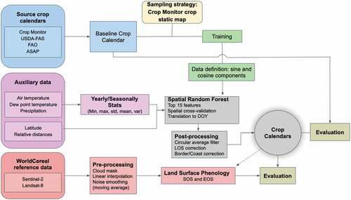
Figure 1 shows a flowchart that summarizes the main steps followed in this study.

Figure 1. Flowchart of the main steps followed in this study. The shapes represent: source data (rounded squares), main processing steps (squares), or outputs (circle). The different colors link the path followed by each data source through the flowchart.

3.1 Existing Crop Calendar Products

Table 1 summarizes the official crop calendar products considered in this work to create the baseline crop calendars More details on each of these products are provided in the following sections.

Table 1. Source and main characteristics of the crop calendar products considered in this study

Crop calendar	Data source	Crop phenological stages^a	Spatial resolution	Temporal resolution	Reference
GEOGLAM Crop Monitor for AMIS	Partners organization analysts, Remote Sensing, USDA-FAS, USDA-NASS, and FAO	5	Administrative Unit	15 days	Becker-Reshef et al. (2019)
ASAP	Remote Sensing, USDA-FAS and FAO	4	Administrative Unit	10 days	Dimou, Meroni, and Rembold (2018)
USDA-FAS	Crop analysts (not documented)	3	National & subnational	15 days	USDA (2006)
FAO	Crop analysts	3	Agro-Ecological Zone	15 days	Sacks et al. (2010)

^aNumber of crops phenological stages recovered by the crop calendar.

3.1.1 Crop Monitor

GEOGLAM has been publishing its monthly CM reports since 2013, in response to the 2011 G20 Agricultural Ministers Action Plan on Price Volatility and Markets (Parihar et al. 2012). These CM reports provide timely, transparent, and actionable information on crop conditions for the four main commodity crops (wheat, maize, rice, soybean) in the major producer/exporting countries. It brings together the international agriculture monitoring community with over 40 contributing organizations that build a multi-source consensus about crop growing conditions, status and agro-climatic conditions likely to impact global production (Becker-Reshef et al. 2019). The information of CM is aggregated at Administrative Unit Level 2 (AU) level, which are homogeneous boundaries based on the AEZ of the FAO Global Administrative Unit Layers (GAUL). In order to create the crop calendars, the CM considered the 5-year average of a complete crop growth cycle, input from partners, remote sensing, and USDA and FAO crop calendars, employing a similar method to the one Sacks et al. (2010). As a result, the CM crop calendars offer information about the stage of the main commodities traded in the international food market. Particularly, the main crop stages that CM provide are as follows: Planting, Early vegetative, Reproductive, Ripening, and Harvest; with 15 days of temporal resolution. Furthermore, it also offers this information for countries at risk of food insecurity through its Crop Monitor for Early Warning (Becker-Reshef et al. 2020).

3.1.2 USDA-FAS

The USDA-FAS (https://ipad.fas.usda.gov/ogamaps/cropcalendar.aspx) International Production and Assessment (IPAD) division has the objective of monitoring the agricultural production of the major commodity crops, as well as assessing food security throughout the world (Fritz et al. 2019; Becker-Reshef et al. 2010). In order to achieve this, USDA-FAS employs a consensus of evidence approach by integrating reports, field surveys, climate data, crop models, and remote sensing data (Becker-Reshef et al. 2010). To support this, USDA-FAS created its own crop calendars based on crop analysts input at national level with a 15-day temporal resolution (as described in Sacks et al. 2010). USDA-FAS SOS and EOS are represented as a period rather than a single date to account for possible local and annual variations.

3.1.3 FAO

Currently, there are two crop calendars generated by FAO: Global Information and Early Warning System (GIEWS), a crop calendar at national-level for the Early Warning countries, and a crop calendar focused on 44 African countries (FAO 2021). In this study, given that most of the information provided by the former is already captured by CM, we used the latter as input to fill in CM gaps in some African countries. This particular calendar is based on crop analysts information and provides data on the planting and harvesting dates for 130 crops, in 283 AEZs, and with a temporal resolution of 15 days (as described in Sacks et al. 2010).

3.1.4 ASAP

The European Commission’s Joint Research Center’s ASAP system offers information about the SOS and the EOS of different crops in 80 priority countries for the European Development Fund and those monitored by GEOGLAM CM for Early Warning (CM4EW, Dimou, Meroni, and Rembold 2018; Rembold et al. 2019). Its crop calendars are downscaled from existing crop calendars (i.e. FAO and USDA-FAS) to national and sub-national levels through LSP metrics. Their objective was to study the link between LSP and crop calendars information. In order to create their own crop calendars, they employed FAO (Fritz et al. 2019), USDA (USDA 2006) and GrisP (GRiSP 2010) crop calendars; crop yield and production data from country statistics, government agencies and FAOSTATS; crop masks from Pérez-Hoyos et al. (2017); and MODIS product MOD13A2v6 over the period 2013–2016. With that information, they detected the main crops and computed their LSP SOS and LSP EOS over the NDVI profile averaged for the period. Then, they confronted LSP SOS and LSP EOS in a scatter plot to create clusters and extracted the start and the end of the LSP SOS and LSP EOS. Finally, they crossed this information with the existing crop calendars SOS and EOS, with a margin of 30 days, to assign a crop type. The final product represents the start and end of the LSP SOS and LSP EOS with a temporal resolution of 10 days, at a national or sub-national level, depending on the area.

3.2. Baseline Maps

The baseline crop calendars are based on the integration of existing crop calendars information: CM, USDA-FAS, FAO and ASAP, in that order of prevalence. This order was decided based on their up-to-date information, documentation, applicability, and methodology. CM’s crop calendars cover a total of four phenological stages. Also, it is based on the best available data from different international agencies, national ministries, and expert knowledge and it has been broadly used (Becker-Reshef et al. 2019). Therefore, this product has been considered as the base map whose missing information is complemented with the other products. ASAP, USDA-FAS, and FAO calendars’ information were considered based on their spatial consistency with the nearby data from CM. The geographical boundaries of each subnational unit of the baseline map, hereafter named as polygons, were inherited from CM and ASAP. When the information was recovered from USDA-FAS and FAO, the administrative units of CM were used.

In this work, the baseline maps served as source of training and validation data to develop the pixel-based crop calendar maps.

3.2.1 Considerations for wheat

Winter wheat crop does not refer to a specific wheat species, but to the timing when wheat is planted (Sacks et al. 2010). In the Northern Hemisphere winter wheat plants go through a winter period with temperatures below 0°C when the crop is generally covered by snow and is dormant. However, some Northern Hemisphere regions (e.g. Canada, northern United States of America (U.S.), northern Europe, Ukraine, Russia, Kazakhstan) also plant spring wheat, whose main difference with winter wheat is that it is planted during the spring and harvested later. In the Southern Hemisphere, winter temperatures are milder, and wheat does not go into dormancy. These differences in the wheat phenological stages require an extra step in the definition of the wheat SOS. In the framework of WorldCereal, we aim to generate a standardized wheat calendar of the Northern and Southern hemispheres. Additionally, note that these calendars are static, and the particular climatology of each year may advance or delay the SOS. Consequently, in this work, we selected the SOS as 1 month before the start of the Vegetative-Productive stage as defined in CM. This means that the selected SOS in the Northern Hemisphere is referred to winter wheat and does not capture the planting date but the end of the dormancy of winter wheat. In the case of USDA-FAS and FAO crop calendars, which provide a range of dates when the SOS happens, we selected a month before the end of the range of SOS to account for the typical delays between planting and emergence of the crop. Regarding the EOS, in CM, USDA-FAS and FAO we selected the average date of the harvest range of dates provided. Finally, given that ASAP is the only product based on EO data, it was only considered when any of the other products was not available for a given region. Looking for consistency between the products and given the range of dates provided by ASAP, we selected within the range the closest date to the nearby regions with calendar data extracted from the other products.

3.2.2 Considerations for maize

Some regions in tropical areas can contain multiple seasons of maize. CM and ASAP include information on two or even three maize growing seasons in some regions. However, since the models are led by climate variables and those regions are generally restricted to tropical areas, the maize calendar presented in this work just focus on one of them. Particularly, we selected the first season defined in CM as the larger producing season (Crop Monitor 2021a) provides a table with information on the season selected for maize), but ensuring maximum consistency with neighboring countries.

To create the baseline SOS and EOS maps of maize, we selected the first date within the range of dates provided in CM, USDA-FAS and FAO; and the most consistent date with the surrounding areas for ASAP.

3.3 Auxiliary data

Table 2 shows a summary of all auxiliary data considered to build our pixel-based crop calendars. The temperature, precipitation and dew point temperature averaged by month were downloaded for the period 1990–2019 from ERA5-Land climate products (ERA5-Land 2021). ERA5-Land products are downscaled from ERA5 products, improving its spatial resolution to 0.1°. Minimum, maximum, average and standard deviation statistics were computed monthly, seasonally, and annually for each product (Muñoz-Sabater et al. 2021). Latitude and longitude of each pixel represented by the x and y coordinates from the geographic projection were also selected as features. Finally, following the methodology of Hengl et al. (2018a), we also considered as features the euclidean distances among the training data. This step is quite important since it will add to the model some non-modeled spatial variation. All the data were resampled to 50 km.

Table 2. Auxiliary data considered in this study

Variable	Source	Resolution	Aggregated
2 m air temperature	ERA-5 Land	0.1°	Month
2 m air dew point temperature	ERA-5 Land	0.1°	Month
Precipitation	ERA-5 Land	0.1°	Month
Latitude	Own-made	0.5°	-
Distances	Own-made	0.5°	-

3.4 WorldCereal reference data

WorldCereal has generated a common input baseline (CIB) which is defined as a database of Analysis Ready Data (ARD) input patch cubes that is used as a reference to train, evaluate and inter-compare the different algorithms. These patch cubes are context-aware stacks of ARD Sentinel-1, Sentinel-2, Landsat 8 and non-EO data, coinciding with the reference data collected. By extracting a large enough context of imagery around each reference data point/polygon, the resulting input patch cubes are ready to serve pixel-based as well as context-based algorithms. Reference samples in the CIB are distributed into calibration/validation/test sets to guarantee their independence and consistency during benchmarking of the different products. The resulting CIB hosts all extracted ARD input patch cubes together with their training labels, and metadata describing the origin of each patch. The CIB is not a static database but evolves simultaneously with the addition of newly collected reference datasets. The CIB used in this work is shown in Table 3, showing that the WorldCereal products have been benchmarked to date for 61,291 samples spread around most continents, although a clear bias is visible toward regions with easily accessible reference data (such as the European LPIS and US crop data layer). Additionally, the html files provided as supplementary materials show the spatial distribution of this dataset. Nevertheless, this CIB provides an unprecedented wealth of agricultural reference samples to evaluate the crop calendars. Note that in this work we just rely on the optical data from Sentinel-2 and Landsat 8 to infer the LSP SOS and LSP EOS validation data as is further described in section 3.8.2.

Table 3. CIB samples’ overview pointing out their respective source dataset, location, date of collection (year), geometry type, and the number of samples present in the CIB

Source	Location	Year	Geometry	Number of samples
LPIS Flanders	Flanders region (Belgium)	2017–2019	POLYGON	8941
LPIS France	France	2017–2019	POLYGON	8796
LPIS Latvia	Latvia	2019	POLYGON	2960
LPIS Austria	Austria	2017–2019	POLYGON	8899
JECAM -Kyiv- Ukraine (NASU-SSAU)	Kyiv oblast (Ukraine)	2019	POLYGON	1029
SIGPAC Catalunya	Catalonia province (Spain)	2019	POLYGON	2978
SIGPAC Andalucia	Andalusia province (Spain)	2019	POLYGON	3094
USDA Crop Data Layer	USA	2019	MAP	14709
Buenos Aires Grain Exchange Argentina	Argentina	2018–2019	POLYGON	3558
Sen2Agri South Sudan	South Sudan	2017	POINT/POLYGON	4505
Gardian PBI India (IFPRI)	India	2017–2018	POINT	943
Gardian OCP Nigeria (IIATA)	Nigeria	2017	POINT	399
RadiantEarth Uganda	Uganda	2017	POLYGON	199
RadiantEarth Tanzania	Tanzania	2018	POLYGON	249
RadiantEarth Kenya	Kenya	2019	POLYGON	32
TOTAL				61,291

3.5 Sampling strategy for the baseline maps

The baseline maps provide constant calendar information through each polygon. However, to generate the model and avoid artifacts caused by over fitting we need to sample the training and validation data. This has been done using as a reference the CM static coarse resolution crop-type maps (Crop Monitor 2021b). These maps represent the percent of each pixel covered by a specific crop at 0.05° resolution (approx. 5.6 km at the equator). For each crop (i.e. wheat and maize), we selected the pixel with the highest percentage of crop inside each polygon. With this approach, we assume that the crop calendar information corresponds to the most representative area within each polygon, and this should be related to the area where the crop is more concentrated, that is, with a higher percentage of crop as defined by the crop-type maps. As a result, the baseline maps’ information was sampled considering a total of 354 samples of wheat (Figure 2a) and 443 samples of maize (Figure 2b). However, these data were not homogeneously distributed in space.

Figure 2. Training (white triangles) and validation (red dots) data selected from the wheat (top) and maize (bottom) baseline maps to build and evaluate the pixel-based maps. Data location shown over the SOS baseline maps.

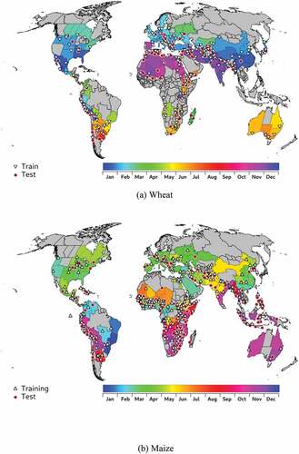
In order to achieve a homogeneous distribution, data was split in 10 groups based on their spatial information. Then, each group was split to three subgroups based on their SOS information, and sampled 10 points inside each subgroup, setting aside the non-selected data for validation purposes. Note that when a subgroup did not meet the minimum requirement of 10 samples, the whole subgroup was selected as training data.

3.6 Crop Calendar data definition

Crop calendars are generally described as the Day Of the Year (DOY) when the SOS or EOS happen. However, DOYs range from 1 (January 1) to 365 (December 31) being DOY 1 and DOY 365 separated only for 1 day. This means that calendars have a circular distribution, and should be treated as such during the modeling process (Mardia and Jupp 2000; Gatto and Jammalamadaka 2015). Following Cremers, we mapped the DOY into a unitary circle, in which each DOY is represented by a unitary vector, a mean direction (i.e. an angle), and sine and cosine components. During the spatial prediction modeling), each component was modeled separately based on the auxiliary data. Finally, the resulting maps of each component were reordered back to a circle by estimating their arc tangent (1) and were translated back to DOY.

(1) $\theta =arctan\frac{sin\theta }{cos\theta }=arctan\frac{f\left(X_{G_{sin\theta }},X_{C_{sin\theta }}\right)}{g\left(X_{G_{cos\theta }},X_{C_{cos\theta }}\right)}$(1)

where θ is the mean direction representing the DOY, sin and cosθ are the predicted sin and cosine components of the mean direction, f(⋅) (and g(⋅)) represent the trained spatial random forest algorithm, whose output is the sine (and cosine) component that defines the calendar dates, and whose inputs are the geographical (X_G) and climate (X_C) features of each model.

3.7 Spatial prediction modeling

Kriging interpolation algorithms are frequently used to build spatial prediction algorithms with good results (Shukla et al. 2020; Xu et al. 2019; Lin et al. 2018; Giustini et al. 2019). However, data must meet the following assumptions (Hengl et al. 2018a; Hengl 2007):

1. Normal distribution of the residuals

2. The variogram must be estimated from the data before the application of the model

3. It is assumed an almost-linear relation among dependent variables and covariates.

Since crop calendar’s data have a circular distribution, it does not meet the first requirement, and it does not ensure the third. As an alternative, our model is based on the methodology presented by (Hengl et al. 2018a) and tested by van den Hoogen et al. (2019) and Hengl et al. (2018b). Basically, we applied a Random Forest algorithm, a robust machine learning algorithm based on ensemble estimates of random decision trees using techniques as bagging (Hengl et al. 2018a; Géron 2019). However, Random Forest doesn’t account for spatial autocorrelation since each observation is considered independent. To overcome this and add a spatial sense into the model, the model was trained with geographical features, more specifically euclidean distances to each point, as proposed by Hengl et al. (2018a).

The spatial Random Forest model considered is based on the Python library sklearn (Pedregosa et al. 2011). Each component describing the crop calendars (i.e. sine and cosine once the data were transformed to circular metrics) was considered independently in the modeling process. In each case, we assessed the importance of each feature (i.e. latitude, climatic variables and distances) based on the permutation feature importance method (Altmann et al., 2010) and selected the top 15. This number was chosen after carefully analyzing the trade-off between error minimization and number of features considered to avoid over fitting. Then, the model was trained based on the selected features, the number of trees, and the maximum depth of each tree. Spatial autocorrelation can generate overfitting of the model (Brenning 2012; Schratz et al. 2019) and underestimate the error. Therefore, we implemented a spatial cross-validation algorithm similar to Brenning (2012). Our algorithm was iterated 10 times, creating 15 spatial groups in each iteration, based on the Leave-One-Group-Out algorithm. Appendix A provides additional information about the features selected. The resulting SOS and EOS maps were finally post-processed to improve spatial and temporal consistency. On the one hand, the resulting maps showed some noise scattered along the coast lines caused by model inaccuracies. This noise was reduced by applying a circular average filter with a moving window of 3 by 3 pixels. On the other hand, looking for the SOS and EOS maps consistency, we computed the Length of Season (LOS) and masked out values with LOS lower than 30 days or greater than 280 days. Finally, we used a circular average with a moving window of 9 by 9 pixels to fill in the masked areas and expand the coast borders.

3.8 Evaluation

We validated the model following two strategies: (1) against the baseline validation samples and (2) against the LSP SOS and LSP EOS, based on the WorldCereal reference data.

3.8.1 Evaluation using baseline data

The sampled dataset was divided into training, used to build the model, and test subsets, which were considered to evaluate the performance of the model. In addition, to inter-compare the predicted crop calendars and the baseline crop calendars, the pixel-based data was aggregated at polygon level but masking out areas with no crop by using as a reference the CM crop-type maps. Note that the cited aggregation at polygon level was done by means of circular averages (Mardia and Jupp 2000). Finally, we computed at each polygon the circular residuals and, from them, the Root Mean Square Error (RMSE) and R² metrics from them.

3.8.2 EO-based evaluation strategy

EO data preprocessing

In this study, the CIB dataset is considered as a reference where EO data is extracted over locations where the crop type is well determined. Based on this dataset, we can apply simple LSP models based on the EO signal, and more specifically optical data, retrieved in each location tagged as wheat or maize to infer the crop calendars information. In this task, we work on surface reflectance data at 10 m resolution retrieved by Sentinel-2 and Landsat 8. They both include a cloud mask which in Sentinel-2 is based on the Sen2Cor scene classification and in Landsat it is based on the FMask algorithm. As pointed out by Baetens et al. (2019), both Sen2Cor and FMask cloud/shadow masks should be dilated to reduce cloud- and shadow-related impurities and drastically boost the quality of the mask. At the same time, pixel-based cloud masks tend to be sensitive to bright surfaces such as certain greenhouse roofs, which are marked as cloudy in the cloud masks. When applying a dilation to these masks, wrongly labeled bright surfaces are smeared out and will mask otherwise clear areas. Therefore, the improved cloud and shadow masking deployed in the WorldCereal system consists of the erosion of the original mask by 30 m to reduce bright surfaces wrongly labeled as clouds and the dilation of the original mask by 200 m to reduce impurities near cloud edges wrongly labeled as clear.

After applying the cloud masking step described above, the resulting images may still present some undetected clouds and shadows, which may negatively impact the optical time series. Therefore, an additional multitemporal gap detection and removal algorithm was implemented (Van Hoolst et al., 2016). This algorithm identifies local minima in time series of NDVI, which exceed a threshold and are hence flagged to be added to the general time-series mask which is then propagated into all individual optical bands of that sensor.

In each location, the CIB extracts EO information over a polygon where the centroid is labeled as a given crop. Therefore, we just extracted the surface reflectance values time series of the central pixel and then, we computed the NDVI from the red and near-infrared bands. Additionally, we computed a 3-daily composite by taking the median reflectance values of all available cloud-free acquisitions in a 6-day moving window. However, the resulting NDVI time-series still presented some noise. Therefore, this noise was smoothed by a moving average with a search window of nine dates. Finally, we filtered out data acquired over locations whose NDVI pattern did not show a consistent NDVI pattern with the neighboring locations by estimating average NDVI profiles within each subnational unit of the baseline map.

LSP method

We developed a simple algorithm to detect and validate the LSP SOS and EOS metrics for wheat and maize crops. It is based on the methodology presented in Jönsson and Eklundh (2004) (Figure 3), where the SOS and EOS are determined based on NDVI thresholds:

Figure 3. Example of NDVI time-series over a maize field in Argentina. The green and the red circle represent the LSP SOS and LSP EOS, respectively; the black triangles point out the local minimums, the white triangle represents the season’s peak, and the shadowed buffer from SOS to EOS highlights the crop’s season.

(2) $NDV{I}_{SOS}=m_{prev}+\left(NDV{I}_{peak}-m_{prev}\right)\cdot p$(2)

(3) $NDV{I}_{EOS}=m_{post}+\left(NDV{I}_{peak}-m_{post}\right)\cdot p$(3)

(4) $m=min\left(NDVI\right)$(4)

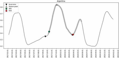
where NDVI_SOS and NDVI_EOS are the NDVI at the SOS and EOS dates; m_prev and m_post are the minimum value of NDVI at the left (previous) and right (posterior) of the peak of the season; p is a constant; and NDVIp_eak is the NDVI value at the peak of the season. Despite Jönsson and Eklundh (2004) set the value of p as 0.1, we set it as 0.2 to ensure that the SOS and the EOS are detected in the correct ranges (i.e. from the minimum to the peak and from the peak to the minimum, respectively). Finally, we selected the closest date of the time-series to the NDVI SOS and NDVI EOS as the SOS and the EOS dates.

However, given the simplicity of the LSP model, we established a time window to apply these equations. Basically, we defined a buffer of ±30 days based on the baseline crop calendars maps when equations 2(2) $NDV{I}_{SOS}=m_{prev}+\left(NDV{I}_{peak}-m_{prev}\right)\cdot p$(2) –4(4) $m=min\left(NDVI\right)$(4) were applied. Next, the resulting LSP SOS and EOS were aggregated at polygon level and were evaluated against the baseline map data. Finally, the proposed pixel-level calendar maps were evaluated against the LSP metrics.

3.8.3 Evaluation metrics

The root mean squared error (RMSE; Géron 2019) and the R² metrics were estimated to assess the performance of the model. The RMSE is defined as

(5) $RMSE=\sqrt{\frac{1}{N}\sum _{i=1}^N{d}_i^2}$(5)

where N is the number of observations, and d_i are linear residuals usually defined as

(6) $d=x-y$(6)

being y the observed values, and the x the predicted values. However, since the distribution of DOY data is circular, we had to modify RMSE metric to deal with circular distances by computing circular residuals instead of linear ones:

(7) $a=\left|x-y\right|$(7)

(8) $b=\left|2\pi -a\right|$(8)

(9) $d_{\circ }=min\left\{a,b\right\}$(9)

obtaining a circular RMSE when combining Equations 5(5) $RMSE=\sqrt{\frac{1}{N}\sum _{i=1}^N{d}_i^2}$(5) –9(9) $d_{\circ }=min\left\{a,b\right\}$(9) :

(10) $RMS{E}_{circ}=\sqrt{\frac{1}{N}\sum _{i=1}^N{d}_{circ}^2}$(10)

Finally, we represented the estimated SOS and EOS maps against the baseline calendars or LSP SOS/LSP EOS metrics using two-dimensional (y = f(x)) plots. While these plots are visual and easy to interpret, this supposes the linearization of a non-linear parameter. Thus, to minimize the error caused by the DOY circular nature and taking advantage of the grouping of the Northern and Southern Hemisphere DOYs (as will be shown in the results section) the observed and predicted values were shifted by a cycle of 2π (i.e. 365 days) forcing some DOYs by the end of the calendar year to have negative values. Particularly, SOS and EOS values greater than 250 days for wheat, and values greater than 210 (SOS) and 350 (EOS) days for maize, were shifted by a cycle (365 days). In this context, the reported R² statistic, which assesses how strong the linear relationship is between two variables and consequently should be taken carefully, is defined in James et al. (2013) as

(11) $R^2=1-\frac{{\sum }_{\hspace{0.17em}}^{\hspace{0.17em}}{d}^2}{{\sum }_{\hspace{0.17em}}^{\hspace{0.17em}}{\left(y-\bar{y}\right)}^2}$(11)

where y is an observation and ȳ is the average of the observations.

4 Results

4.1 Wheat

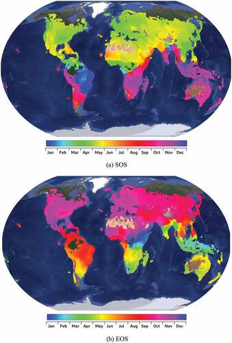
Figure 4(a, b)) shows the SOS and EOS predicted maps masking out the non-cropland areas using the Copernicus Land Cover product. In the case of the SOS, we can distinguish four main behaviors in terms of geographical locations: the Northern Hemisphere, the Mediterranean basin, and its surroundings down to the Equator, the effect of the tropics and the rainforests area, and the Southern Hemisphere. The Northern Hemisphere SOS after dormancy generally spans from January to April. However, surrounding the Mediterranean basin and the across Middle East, the planting dates span from November to February. In equatorial areas such as North Africa, the planting dates span from December to August, while in Central America and the North of South America, the planting dates span from March to April. Finally, in the Southern Hemisphere, the planting dates span from April to August.

Figure 4. Wheat crop calendar maps over a base map from the Google Earth dataset. Locations with no agricultural areas are excluded. Furthermore, the color legend is circular, meaning that the blue color of December 31 matches the blue color of January 1.

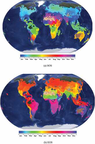
There are three general patterns for wheat EOS (Figure 4b): the homogeneous pattern in the Northern Hemisphere, whose dates increase as latitude decrease; the equatorial area, with different pattern in America, North and South Africa and Asia; and the Southern Hemisphere, where Argentina and Chile, Southern Africa and Oceania show different dates. Specifically, in the Northern Hemisphere, including the Mediterranean basin, the dates span from April to July; in the equatorial area, the dates span from August to October in central and south America, in Africa from December to May at the north of the Equator and from October to March at the south, and in Asia from March to April. The Southern Hemisphere shows a heterogeneous pattern: dates in the north of Argentina spans from November to December, while in the south from June to July; in Chile, the harvesting dates span from March to July; in the South of Africa, the dates span from September to November; and in Australia and New Zealand the harvesting dates span from October to January; and Indonesia, the dates span from July to August.

4.1.1 Evaluation

Evaluation using baseline data

Figure 5 shows the evaluation of the modeled crop calendars with the baseline data set aside for validation purposes and Figure 6 shows the spatial distribution of the residuals. The SOS evaluation (Figure 5a) shows an R² of 0.87 and an RMSE of 27 days. Figure 6a shows that most of the residuals (over 85%) are lower than 30 days. However, there are two major outliers where the baseline provides a SOS around DOY 200 and the modeled maps show values around 1. Looking at Figure 6a these two polygons are located in Tanzania and Yemen, where the lack of data forces the extrapolation of the model. Additionally, there are some cases, represented in the scatter plot with horizontal lines, where the model shows some variability whilst the baseline provides constant SOS.

Figure 5. Wheat crop calendar evaluation at polygon scale.

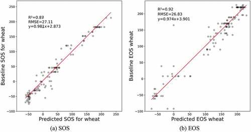
Figure 6. Wheat residuals at polygon scale.

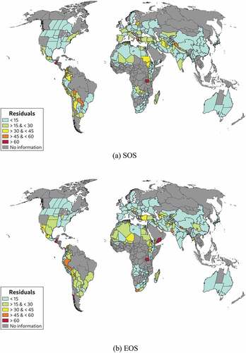
Figure 5b shows the evaluation of the EOS maps with an R² of 0.92 and an RMSE of 26 days. The residual map (Figure 6b) shows that 82% of them are lower than 30 days. However, there are some residuals larger than 60 days (less than 3%) and are located in Guatemala, Chile, Tanzania and Yemen (outliers in Figure 5b). Additionally, in Figure 6b, there is some horizontal data with baseline EOS around the beginning of the year, while the modeled EOS provides a variation from DOY 325 (−40 in the plot) to DOY 50.

EO-based evaluation

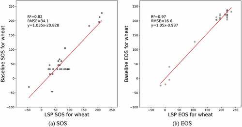
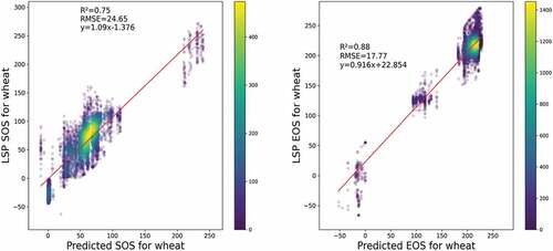
The supplementary material provides a html file where the reader can explore spatially the wheat sites within the CIB, select a given site, and check its corresponding wheat NDVI seasonal curve (highlighted in gray) and the resulting LSP SOS and LSP EOS metrics (red dots). Figure 7 shows the evaluation of all these LSP metrics (i.e. SOS and EOS) against the baseline crop calendars values by aggregating the LSP singular values to polygon level. As discussed in the Introduction section, a bias was expected between both datasets caused by the different crop development stages that each of them represents. In fact, the LSP metrics were corrected for a constant shift of −20 days in the case of the LSP SOS and +27 days in the case of the EOS LSP. These bias values were extracted from the linear regression’s intercept of the baseline vs LSP metrics before correcting the shift. The LSP SOS explains 82% of the variance, while the LSP EOS explains 97% of the variance. However, the SOS evaluation shows a horizontal pattern along DOY 40, that is caused by the baseline crop calendars constant values, while the LSP metrics show some variability. These discrepancies are located across northern states in the US where CM shows constant dates of the transition to vegetative phase.

Figure 7. Wheat LSP SOS and EOS evaluation against baseline.

After the successful LSP model evaluation with the baseline data, these results were then considered to evaluate the modeled SOS and EOS maps with the computed LSP SOS and EOS (Figure 8). The predicted SOS explains 75% of the variance of the LSP SOS with an RMSE of 25 days, while the EOS explains 88% of the variance and an RMSE of 18 days. There are vertical lines indicating generalization of the predicted SOS with respect to the LSPs. This might be caused either by the inter-annual LSP metrics variation (note that the CIB contains data from 2017 to 2021) or because there is an actual variation of the calendars that the model cannot capture.

Figure 8. Wheat SOS and EOS modeled maps evaluation against LSP metrics. The colors represent the data density.

4.2 Maize

Figure 9 shows the predicted SOS and EOS dates for maize masking out the non-cropland areas using the Copernicus Land Cover product. Maize maps show a more constant pattern than wheat in both SOS and EOS. At this point we must keep in mind that the SOS of wheat in the Northern Hemisphere represents the winter wheat emergence after dormancy. Thus, the variability of the wheat SOS, and consequently EOS, is linked to the winter temperatures in each area. In the SOS (Figure 9a), the map shows three different patterns in the Northern Hemisphere, the west and the east of the Southern Hemisphere. Specifically, in the Northern Hemisphere the SOS span from April to May, from August to December in the west of Southern Hemisphere, and from August to late November in the east of the Southern Hemisphere. However, there are some dates that do not match these rules, such as the dates of December and January in Indonesia; about April and May in Vietnam, Philippines and Venezuela; and from February to March in the equatorial west of Africa.

Figure 9. Maize crop calendar dates over a base map from the Google Earth dataset. Locations with no agricultural areas are excluded. Furthermore, the color legend is circular, meaning that the blue color of December 31 matches the blue color of January 1.

In the case of the EOS (Figure 9b), the global pattern is more continuous. Generally, we can split the results into three areas, the Northern Hemisphere, the west of the Southern Hemisphere and the east of the Southern Hemisphere. In the Northern Hemisphere, the dates span from July to November, without considering the area of Malaysia; in the west of the Southern Hemisphere the dates span from May to November, although the latter can be a consequence of the extrapolation; and in the east of the Southern Hemisphere, including Malaysia, the EOS span from December to June, with the latter days over Australia and New Zealand.

4.2.1 Evaluation

Evaluation using baseline data

Figure 10 shows the evaluation of the modeled metrics against the baseline data at polygon level, while Figure 11 shows the spatial distribution of the residuals. Maize SOS results (Figure 10a) show a good agreement with an R² of 0.88 and RMSE of 24 days. Over 87% of residuals of the SOS (Figure 11a) are lower than 30 days and only 3% are larger than 60 days, and are located in the south of Brazil, Congo, Angola, Uganda, Saudi Arabia, India, Thailand and Philippines.

Figure 10. Maize R² evaluation at polygon scale.

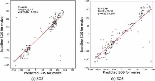
Figure 11. Maize residuals at polygon scale.

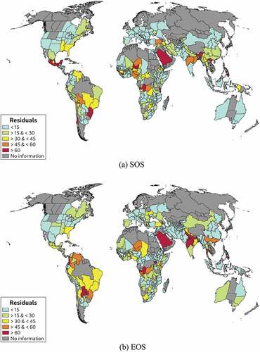
Maize’s EOS evaluation (Figure 10b) shows an R² of 0.79 and an RMSE of 28 days. Note that the low R² is mainly caused by the data in the bottom right area, which do not fit well to a linear model while dates are closer in a circular context. Note that the data represented in Figures 10a and 10b are grouped in two main clusters, which refer to the Northern and Southern Hemisphere data. Looking at the residuals map (Figure 11b), most of the residuals (88%), and mainly in the Northern Hemisphere, are lower than 30 days. However, compared to the previous maps’ analysis, it shows the largest percentage of the residuals with values greater than 60 days (4%). These errors are located in Mexico, Brazil, Chile, Guinea, Nigeria, Congo, Saudi Arabia, Thailand, Vietnam and Philippines.

The source of the high residual errors in some areas is heterogeneous. In Brazil, Saudi Arabia and India, the errors are linked to the large size of the polygons, where the baseline maps provide a constant calendar data while the climate data show very different climate patterns. Meanwhile, in other areas such as Congo or Guinea, the model cannot describe the calendar dates. These areas are generally located in the Tropics, where the SOS and EOS dates might be better explained by other socioeconomic factors rather than climatology.

EO-based evaluation

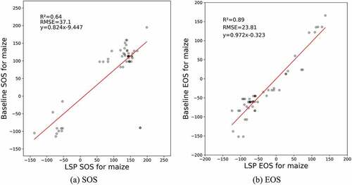
Similar to wheat, the supplementary material provides a html file where the reader can explore spatially the maize sites within the CIB, select a given site, and check its corresponding maize NDVI seasonal curve (highlighted in gray) and the resulting LSP SOS and LSP EOS metrics (red dots). Figure 12 shows the evaluation of all these LSP metrics with the baseline crop calendars. As discussed in the previous section, the direct comparison of both datasets shows a constant bias that has been corrected in these plots by shifting +8 days the LSP SOS and +15 the LSP EOS. The SOS evaluation shows an RMSE of 37 days and an R² of 0.64, while the EOS evaluation shows an RMSE of 24 days and an R² of 0.89. Also in this case, the observations are split into two groups that reference the Northern and Southern concentrations of the baseline crop calendar.

Figure 12. Maize LSP SOS and LSP EOS evaluation against baseline.

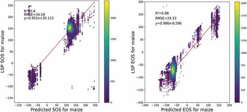
Figure 13 shows the evaluation of the modeled SOS and EOS maps with the LSP metrics considering the aforementioned bias correction. The results show that the proposed maps can explain 80% of the LSP SOS variance with an RMSE of 35 days; and they can explain 88% of the LSP EOS variance with an RMSE of 24 days. In this case, there are some vertical patterns that show LSP variance while the proposed maps remain constant.

Figure 13. Maize SOS and EOS modeled maps evaluation against LSP metrics. The colors represent the data density.

5 Discussion

In this work, we inferred continuous (pixel-based) global wheat and maize crop calendar maps based on discrete information from existing global crop calendar products and meteorological data. First, we built a baseline map by combining the information provided by the existing products. CM was considered as the basemap and the other products complemented its information over the missing areas. Special attention was put toward the different products’ consistency in definition and temporal and spatial resolutions. This was a challenging task given the range of dates that each product considers to define the SOS or the period between planting and vegetative phase. In fact, according to Whitcraft, Becker-Reshef, and Justice (2015b), crop calendars are generally outdated and poorly documented, leading to a lack of confidence in the accuracy of the planting and harvesting dates. In the framework of WorldCereal, whose main objective is building robust wheat and maize classification algorithms and looking for coherence of the wheat’s SOS definition across the Northern and Southern Hemisphere, we defined the SOS as 1 month prior to the beginning of the vegetative phase. As explained in the Materials and methods section, we selected this period of time after computing the average time period between planting and the vegetative stage of wheat in the Southern Hemisphere based on CM, which was estimated as 2 months. Note that the products considered in the baseline map provided the data in time frames of 10 or 15 days. Therefore, in the framework of the WorldCereal project where these maps will be used by the classification algorithms, 30 days before the vegetative stage ensures that, independently on the yearly weather variation, the plant has not emerged yet. However, this selection, that provides consistency between the Northern and Southern hemisphere, omits the winter wheat period before dormancy in the Northern hemisphere.

Second, the baseline SOS and EOS maps are generalized through the different countries or subnational units (polygons). Therefore, the baseline maps were sampled by assuming that the calendar information within each polygon is representative of the area where the given crop is predominant. This was achieved by using as a reference the static crop-specific masks from CM and representing the percent of each pixel covered by a specific crop. We acknowledge that assigning to a given area the average crop calendar dates of the whole region might be biased in in countries with large agricultural regions. For example, in the Middle East countries where the climate conditions in the same period have considerable differences through the north to south or east to west, the crops’ (i.e. wheat and maize) SOS and EOS and their classification patterns should be different. This is in fact the major source of error causing the high residuals in the maize calendars across the Middle East and India. However, this is the best information currently available.

Third, we built a model to capture the calendar’s spatial variability mainly based on meteorological data (dew point temperature and precipitation). However, Sacks et al. (2010) explained that in some cases socioeconomic and cultural aspects have a strong impact on the crop calendars. Looking at the features’ importance (Appendix A), climate variables have a greater weight in the wheat components, but this is not the case for maize models, where the features’ importance is lower and more homogeneously distributed. This could be the consequence of the low variability of the baseline calendars in the Northern Hemisphere. The main advantage of the proposed model is that given its simplicity it could be easily applied to infer crop calendars of other annual crops.

In the evaluation of the model based on a test subset of the baseline maps, the results show that a model based on non-linear modeling of crop calendar’s information at global scale shows good performance metrics with SOS (EOS) R² of 0.87 (0.92) and an RMSE of 27 (26) days for wheat and SOS (EOS) R² of 0.88 (0.79) and an RMSE of 24 (28) days for maize. These metrics show the good performance of the presented products when compared to previous works in the literature such as Stehfest et al. (2007), whose results showed an R² of 0.67 for wheat and 0.66 for maize planting dates. However, these metrics are limited to areas with available data. Hence, any calendar information outside these zones must be taken carefully, especially in the tropics where errors are larger according to the residual maps shown in Figures 6 and 11. This might be a consequence: of the lack of data available to train the models, their multiple agricultural seasons, and their lower dependency on the climatology (main driver of our model). Also, in large countries or subnational units with diverse agricultural conditions and very limited information such as the Middle East and India as mentioned above. Additionally, higher latitudes and isolated isles are generated based purely on extrapolation and buffering. Thus, these areas are expected to have high uncertainties. We must note the limited information available on crop calendars to build a strong baseline of well-distributed training samples.

Given that fine-scale ground data are not available, we examined reported crop calendars in the literature. Next, we highlight some cases where there are some discrepancies among products. In Tanzania, where the literature and the proposed calendars define the wheat SOS in April, the baseline points out the SOS earlier in December. In fact, this is the largest residual (difference between modeled and baseline SOS) in Africa shown in Figure 6. This inconsistency can be explained by the fact that in this particular polygon, the baseline shows a very different SOS compared to the neighboring countries. Therefore, the model used to generate the proposed calendars provided a stronger weight to the consistency across the neighboring countries, providing a more accurate crop calendar estimation. In Nepal, both the baseline maps and the proposed calendars match the dates reported in the literature (Thapa et al. 2020) excepting the EOS of the western region, where the baseline agrees with the reported calendar while the proposed calendars are shifted from 30 to 50 days. Finally, in southern Brazil (Becker et al. 2020), both datasets SOS are shifted 2 months compared to the reported calendars, while the EOS is shifted 1 month.

Finally, the calendar maps were also evaluated based on the outputs from a simple LSP model based on Sentinel-2 observations over in-situ reference samples whose crop type is known. Given the simplicity of the LSP model considered the SOS and EOS detection might show some inaccuracies. However, building a strong LSP model is out of the scope of this work and the LSP data is just considered as an additional evaluation dataset of the proposed maps. Looking at the NDVI seasonal evolution across the different sites of the CIB (supplementary materials) the considered LSP model generally captures well the LSP SOS and LSP EOS both for wheat and maize. The resulting data derived from the LSP model was aggregated at polygon level and was evaluated against the baseline dataset. These datasets showed a SOS (EOS) bias of 20 (27) days in wheat and 8 (15) days in maize. This is a direct consequence of how the SOS or EOS is defined in each product and the shift considered in each case to linearize the circular calendar dates. While the proposed maps consider the SOS as one month before the vegetative phase, the LSP metrics detect the presence of vegetation and therefore are detecting a crop stage well within the vegetative phase. Reversely, the EOS as defined in the baseline considers the average date within the harvest dates, while the LSP metrics detect the senescence of vegetation. When correcting this constant bias, the evaluation showed a good consistency in both crops with an RMSE of 34 (17) days and an R² of 0.82 (0.97) for wheat SOS (EOS) and an RMSE of 37 (24) days and an R² of 0.64 (0.89) for maize SOS (EOS). However, there are some cases where the baseline data remain constant while the LSP metrics do not. This might be a consequence of socio-economic factors (that explain a large spread in LSP), the errors generated by the simple LSP model considered, the presence of errors in the in-situ reference data or the wide range of dates between the planting and vegetative phase (and the ripening through harvest phase) that the existing products currently have which minimizes the spatial variation between polygons. Once evaluated, this data was then used to evaluate the predicted calendar maps. This evaluation showed a SOS (EOS) R² of 0.75 (0.88) and an RMSE of 25 (18) days for wheat and a SOS (EOS) R² of 0.80 (0.88) and an RMSE of 35 (24) days for maize. These results are consistent with the evaluation based on the baseline test dataset. While the different crops and season showed equivalent R², the SOS evaluation errors were higher than the EOS errors and maize showed higher errors than wheat. The higher errors found in the SOS maps when compared to EOS can be a consequence of the larger variability of the planting date when compared to the harvesting date. Meanwhile, maize shows higher errors than wheat given the larger amount of data analyzed and their wider spatial distribution. Additionally, the performance metrics are well aligned to other studies found in the literature such as Mishra et al. (2021), whose results based on rice crop calendars showed SOS and EOS estimations with an R² of 0.88 and 0.82, and an RMSE of 34.2 days and 46.5 days, respectively. Despite the overall good metrics there are still some discrepancies that can be caused by the yearly meteorological variations, which are captured by the LSP metrics but are not represented in the static calendar maps. Additionally, the horizontal pattern found in Figure 7a corresponds to SOS data across the US and Europe and are caused by the stability of the baseline SOS crop calendars whilst the LSP SOS show a variation that can get to 100 days.

The presented model is novel, and with the collaboration of the agricultural communities around the world to increase the quantity and quality of the reference data, and with the integrated use of ground and EO data, it would be feasible to obtain more precise outputs. Particularly, LSP maps could be used to improve the resolution of the calendars and their accuracy in some regions where there is a lack of information. However, while there are many different methods to infer LSP metrics, if they are crop specific, they need to rely on crop-type maps. WorldCereal will produce those at global scale and at fine spatial resolution. However, this project will rely on the current crop calendars first, to trigger the algorithms within 1 month after the EOS and second to normalize the metrics with the accumulated GDD from the SOS. Thus, in future studies, these maps can be improved in an iterative way with the WorldCereal crop-type maps.

As a summary and replying to the science questions stated in the introduction section, in this work we have successfully applied a spatial Random Forest algorithm to exploit the current crop calendar datasets available and build SOS and EOS winter wheat and maize calendars that provide continuous spatial variability (replying to Q1). Regarding validation, given the scarcity of existing ground data and calendars, as well as their unknown accuracy, it is very challenging to evaluate our calendars in a rigorous way. In this context, a simple LSP model based on EO data acquired over already known crop types, was a useful source to evaluate those maps, though as discussed above there are some limitations that should be considered (LSP model errors and misclassification of the data) (replying to Q2).

Data availability statement

The four crop calendar maps created in this study are available through the GitHub repository https://github.com/ucg-uv/research_products/tree/main/cropcalendars.

Disclosure statement

No potential conflict of interest was reported by the author(s).

Supplementary material

Supplemental data for this article can be accessed online at https://doi.org/10.1080/15481603.2022.2079273

Additional information

Funding

This study was funded by the ESA WorldCereal project (4000130569/20/I-NB) and by the program Generacio Talent of Generalitat Valenciana (CIDEGENT/2018/009);Conselleria de Innovación, Universidades, Ciencia y Sociedad Digital, Generalitat Valenciana.

Appendix A.

Model Features

A.1 Wheat

Figure A1: Top 15 most important features of the random forest regressor for the sine component of the wheat’s SOS.

Figure A2: Top 15 most important features of the random forest regressor for the cosine component of the wheat’s SOS.

Figure A3: Top 15 most important features of the random forest regressor for the sine component of the wheat’s EOS.

Figure A4: Top 15 most important features of the random forest regressor for the cosine component of the wheat’s EOS.

A.2 Maize

Figure A5: Top 15 most important features of the random forest regressor for the sine component of the maize’s SOS.

Figure A6: Top 15 most important features of the random forest regressor for the cosine component of the maize’s SOS.

Figure A7: Top 15 most important features of the random forest regressor for the sine component of the maize’s EOS.

Figure A8: Top 15 most important features of the random forest regressor for the cosine component of the maize’s EOS.

References

- Altmann, A., L. Toloşi, O. Sander, and T. Lengauer. 2010. “Permutation Importance: A Corrected Feature Importance Measure.” Bioinformatics 26 (10): 1340–1347.
- Atzberger, C. February 2013. “Advances in Remote Sensing of Agriculture: Context Description, Existing Operational Monitoring Systems and Major Information Needs.” Remote Sensing 5 (2): 949–981. 2072-4292. http://www.mdpi.com/2072-4292/5/2/949
- Baetens, L., C. Desjardins, and O. Hagolle. 2019. “Validation of Copernicus Sentinel-2 Cloud Masks Obtained from MAJA, Sen2cor, and Fmask Processors Using Reference Cloud Masks Generated with a Supervised Active Learning Procedure.” Remote Sensing 11 (4): 433.
- Banerjee, A., and D. S. Dawn. 2020. “Preparation of Crop Calendar on Mangalbari Town under Matiali Block, Jalpaiguri District.” Agriculture Journal IJOEAR 6 (12): 10.
- Becker, W. B., J. Richetti, E. Mercante, J. C. Esquerdo, C. A. Silva, A. Paludo, and J. A. Johann. August 2020. “Agricultural Soybean and Crop Calendar Based on Moderate Resolution Satellite Images for Southern Brazil.” Semina: Ciências Agrárias 41: 2419–2428. 16790359. http://www.uel.br/revistas/uel/index.php/semagrarias/article/view/37964
- Becker, W. B., L. Silva, J. Richetti, T. Ló, and J. Johann. February 2021. “Harvest Date Forecast for Soybeans from Maximum Vegetative Development Using Satellite Images.” International Journal of Remote Sensing 42: 1121–1138. 0143-1161. https://www.tandfonline.com/doi/full/10.1080/01431161.2020.1823042
- Becker-Reshef, I., C. Justice, M. Sullivan, E. Vermote, C. Tucker, A. Anyamba, J. Small, et al. June 2010. “Monitoring Global Croplands with Coarse Resolution Earth Observations: The Global Agriculture Monitoring (GLAM) Project.” Remote Sensing 2 (6): 1589–1609. 2072-4292. http://www.mdpi.com/2072-4292/2/6/1589
- Becker-Reshef, I., B. Franch, B. Barker, E. Murphy, A. Santamaria-Artigas, M. Humber, S. Skakun, and E. Vermote. October 2018. “Prior Season Crop Type Masks for Winter Wheat Yield Forecasting: A US Case Study.” Remote Sensing 10 (10): 1659. 2072-4292. http://www.mdpi.com/2072-4292/10/10/1659
- Becker-Reshef, I., B. Barker, M. Humber, E. Puricelli, A. Sanchez, R. Sahajpal, K. McGaughey, et al. December 2019. “The GEOGLAM Crop Monitor for AMIS: Assessing Crop Conditions in the Context of Global Markets.” Global Food Security 23: 173–181. 22119124. https://linkinghub.elsevier.com/retrieve/pii/S221191241830155X
- Becker-Reshef, I., C. Justice, B. Barker, M. Humber, F. Rembold, R. Bonifacio, … J. Verdin. 2020. “Strengthening Agricultural Decisions in Countries at Risk of Food Insecurity: The GEOGLAM Crop Monitor for Early Warning.” Remote Sensing of Environment 237: 111553. doi:10.1016/j.rse.2019.111553.
- Benami, E., Z. Jin, M. R. Carter, A. Ghosh, R. J. Hijmans, A. Hobbs, B. Kenduiywo, and D. B. Lobell. February 2021. “Uniting Remote Sensing, Crop Modelling and Economics for Agricultural Risk Management.” Nature Reviews Earth & Environment 2 (2): 140–159. 2662-138X http://www.nature.com/articles/s43017-020-00122-y
- Bornez, K., A. Descals, A. Verger, and J. Peñuelas. 2020. “Land Surface Phenology from VEGETATION and PROBA-V Data. Assessment Over Deciduous Forests.” International Journal of Applied Earth Observation and Geoinformation 84: 101974.
- Bórnez, K., A. Descals, A. Verger, and J. Peñuelas. February 2020. “Land Surface Phenology from VEGETATION and PROBA-V Data. Assessment over Deciduous Forests.” International Journal of Applied Earth Observation and Geoinformation 84: 101974. 03032434 https://linkinghub.elsevier.com/retrieve/pii/S0303243419301278
- Brenning, A. “Spatial cross-validation and Bootstrap for the Assessment of Prediction Rules in Remote Sensing: The R Package Sperrorest.” In 2012 IEEE International Geoscience and Remote Sensing Symposium, 5372–5375, Munich, Germany, July 2012. IEEE. doi: 10.1109/IGARSS.2012.6352393.
- Caparros-Santiago, J. A., V. Rodriguez-Galiano, and J. Dash. January 2021. “Land Surface Phenology as Indicator of Global Terrestrial Ecosystem Dynamics: A Systematic Review.” ISPRS Journal of Photogrammetry and Remote Sensing 171: 330–347. 09242716. https://linkinghub.elsevier.com/retrieve/pii/S0924271620303269
- Crop Monitor. “Classification System.” 2021a. https://cropmonitor.org/index.php/crop-conditions/classification-systems/
- de Castro, A., J. Six, R. Plant, and J. Peña. November 2018. “Mapping Crop Calendar Events and Phenology-Related Metrics at the Parcel Level by Object-Based Image Analysis (OBIA) of MODIS-NDVI Time-Series: A Case Study in Central California.” Remote Sensing 10 (11): 1745. 2072-4292 http://www.mdpi.com/2072-4292/10/11/1745
- Descals, A., A. Verger, G. Yin, and J. Penuelas. 2021. “A Threshold Method for Robust and Fast Estimation of land-surface Phenology Using Google Earth Engine.” IEEE Journal of Selected Topics in Applied Earth Observations and Remote Sensing 1. 1939-1404, 2151-1535 https://ieeexplore.ieee.org/document/9265265/
- Dimou, M., M. Meroni, and F. Rembold. 2018. Development of a National and sub-national Crop Calendars Data Set Compatible with Remote Sensing Derived Land Surface Phenology: Technical Description of the Selection Method Used for Building the Crop Calendars Data Set of the Anomaly Hot Spots of Agricultural Production (ASAP). LU: Publications Office. https://data.europa.eu/doi/10.2760/25859
- ERA5-Land, 2021. European Centre for Medium-Range Weather Forecasts. Accesed the 10th of December of 10th December 2021. https://www.ecmwf.int/en/era5-land
- FAO. “Climate Change and Food Security: A Framework Document.” FAO, Viale delle Terme di Caracalla 00153 Rome, Italy, 2008. https://www.fao.org/3/k2595e/k2595e00.htm
- FAO. “Climate Change and Food Security: Risks and Responses.” FAO, 2015. https://www.fao.org/documents/card/en/c/82129a98-8338-45e5-a2cd-8eda4184550f/
- FAO. “FAO Crop Calendar.” 2021. https://cropcalendar.apps.fao.org/home
- Franch, B., E. F. Vermote, I. Becker-Reshef, M. Claverie, J. Huang, J. Zhang, and J. A. Sobrino. 2015. “Improving the Timeliness of Winter Wheat Production Forecast in the United States of America, Ukraine and China Using MODIS Data and NCAR Growing Degree Day Information.” Remote Sensing of Environment 161: 131–148.
- Franch, B., E. Vermote, S. Skakun, J. Roger, I. Becker-Reshef, E. Murphy, and C. Justice. April 2019. “Remote Sensing Based Yield Monitoring: Application to Winter Wheat in United States and Ukraine.” International Journal of Applied Earth Observation and Geoinformation 76: 112–127. 03032434. https://linkinghub.elsevier.com/retrieve/pii/S0303243418306536
- Franch, B., E. Vermote, S. Skakun, A. Santamaria-Artigas, N. Kalecinski, J.-C. Roger, I. Becker-Reshef, B. Barker, C. Justice, and J. Sobrino. December 2021. “The ARYA Crop Yield Forecasting Algorithm: Application to the Main Wheat Exporting Countries.” International Journal of Applied Earth Observation and Geoinformation 104: 102552. 03032434. https://linkinghub.elsevier.com/retrieve/pii/S0303243421002592
- Fritz, S., L. See, J. C. L. Bayas, F. Waldner, D. Jacques, I. Becker-Reshef, A. Whitcraft, et al. January 2019. “A Comparison of Global Agricultural Monitoring Systems and Current Gaps.” Agricultural Systems 168: 258–272. 0308521X. https://linkinghub.elsevier.com/retrieve/pii/S0308521X17312027
- Garcia-Perez, M. A., L. Quesada-Ruiz, J. A. Caparros-Santiago, E. Sánchez-Rodríguez, and V. Rodriguez-Galiano. September 2021. “A Case of Study of Land Surface Phenology for CAP Management: Using Sentinel-2 Data to Obtain Phenometrics for Winter Cereals in Andalusia, Spain.” In Remote Sensing for Agriculture, Ecosystems, and Hydrology XXIII, edited by C. M. Neale and A. Maltese, 6. Online Only, Spain: SPIE. doi:10.1117/12.2600114.
- Gatto, R., and S. R. Jammalamadaka. March 2015. “Directional Statistics: Introduction.” In Wiley StatsRef: Statistics Reference Online, edited by N. Balakrishnan, T. Colton, B. Everitt, W. Piegorsch, F. Ruggeri, and J. L. Teugels, 1–8. Chichester, UK: John Wiley & Sons, . doi:10.1002/9781118445112.stat00201.pub2.
- Géron, A. 2019. Hands-On Machine Learning with Scikit-Learn, Keras, and Tensorflow: Concepts, Tools, and Techniques to Build Intelligent Systems. second ed. USA: O’Reilly Media.
- Giustini, F., G. Ciotoli, A. Rinaldini, L. Ruggiero, and M. Voltaggio. April 2019. “Mapping the Geogenic Radon Potential and Radon Risk by Using Empirical Bayesian Kriging Regression: A Case Study from A Volcanic Area of Central Italy.” Science of the Total Environment 661: 449–464. 00489697. https://linkinghub.elsevier.com/retrieve/pii/S0048969719301640
- Godfray, H. C. J., J. R. Beddington, I. R. Crute, L. Haddad, D. Lawrence, J. F. Muir, J. Pretty, S. Robinson, S. M. Thomas, and C. Toulmin. February 2010. “Food Security: The Challenge of Feeding 9 Billion People.” Science 327 (5967): 812–818. 0036-8075, 1095-9203. https://www.science.org/doi/10.1126/science.1185383
- GRiSP. “Global Rice Science Partnership.” 2010.
- Helman, D. March 2018. “Land Surface Phenology: What Do We Really ‘See’ from Space?” Science of the Total Environment 618: 665–673. 00489697. https://linkinghub.elsevier.com/retrieve/pii/S004896971731954X
- Hengl, T.2007.European Commission, Joint Research Centre, and Institute for Environment and Sustainability (Ispra, I. A Practical Guide to Geostatistical Mapping of Environmental Variables.Luxembourg: Publications Office.
- Hengl, T., M. Nussbaum, M. N. Wright, G. B. Heuvelink, and B. Gräler. August 2018a. “Random Forest as a Generic Framework for Predictive Modeling of Spatial and spatio-temporal Variables.” PeerJ 6: e5518. 2167-8359. https://peerj.com/articles/5518
- Hengl, T., M. G. Walsh, J. Sanderman, I. Wheeler, S. P. Harrison, and I. C. Prentice. August 2018b. “Global Mapping of Potential Natural Vegetation: An Assessment of Machine Learning Algorithms for Estimating Land Potential.” PeerJ 6: e5457. 2167-8359. https://peerj.com/articles/5457
- Hsiao, T. C., L. Heng, P. Steduto, B. Rojas-Lara, D. Raes, and E. Fereres. May 2009. “AquaCrop-The FAO Crop Model to Simulate Yield Response to Water: III. Parameterization and Testing for Maize.” Agronomy Journal 101 (3): 448–459. 00021962. http://doi.wiley.com/10.2134/agronj2008.0218s
- Jägermeyr, J., C. Müller, A. C. Ruane, J. Elliott, J. Balkovic, O. Castillo, B. Faye, et al. November 2021. “Climate Impacts on Global Agriculture Emerge Earlier in New Generation of Climate and Crop Models.” Nature Food 2 (11): 873–885. 2662-1355. https://www.nature.com/articles/s43016-021-00400-y
- James, G., D. Witten, T. Hastie, and R. Tibshirani. 2013. An Introduction to Statistical Learning, Volume 103 of Springer Texts in Statistics. New York, New York, NY: Springer. doi:10.1007/978-1-4614-7138-7.
- Javed, M. A., S. Rashid Ahmad, W. K. Awan, and B. A. Munir. March 2020. “Estimation of Crop Water Deficit in Lower Bari Doab, Pakistan Using Reflection-Based Crop Coefficient.” ISPRS International Journal of Geo-Information 9 (3): 173. 2220-9964. https://www.mdpi.com/2220-9964/9/3/173
- Jeong, S. J., C. H. HO, H. J. Gim, and M. E. Brown. 2011. “Phenology Shifts at Start Vs. End of Growing Season in Temperate Vegetation over the Northern Hemisphere for the Period 1982–2008.” Global Change Biology 17 (7): 2385–2399. doi:10.1111/j.1365-2486.2011.02397.x.
- Jönsson, P., and L. Eklundh. October 2004. “TIMESAT—a Program for Analyzing time-series of Satellite Sensor Data.” Computers & Geosciences 30 (8): 833–845. 00983004. https://linkinghub.elsevier.com/retrieve/pii/S0098300404000974
- Kogan, F., N. Kussul, T. Adamenko, S. Skakun, O. Kravchenko, O. Kryvobok, A. Shelestov, A. Kolotii, O. Kussul, and A. Lavrenyuk. August 2013. “Winter Wheat Yield Forecasting in Ukraine Based on Earth Observation, Meteorological Data and Biophysical Models.” International Journal of Applied Earth Observation and Geoinformation 23: 192–203. 03032434. https://linkinghub.elsevier.com/retrieve/pii/S0303243413000123
- Kyu Lee, S., and T. An Dang. June 2020. “Crop Calendar Shift as a Climate Change Adaptation Solution for Cassava Cultivation Area of Binh Thuan Province, Vietnam.” Pakistan Journal of Biological Sciences 23 (7): 946–952. 10288880. https://www.scialert.net/abstract/?doi=pjbs.2020.946.952
- Lin, J., A. Zhang, W. Chen, and M. Lin. August 2018. “Estimates of Daily PM2.5 Exposure in Beijing Using Spatio-Temporal Kriging Model.” Sustainability 10 (8): 2772. 2071-1050. http://www.mdpi.com/2071-1050/10/8/2772
- Mardia, K. V., and P. E. Jupp.2000.Directional Statistics. Wiley Series in Probability and Statistics.Chichester; New York: J. Wiley.
- Mbow, C., C. Rosenzweig, L. G. Barioni, T. G. Benton, M. Herrero, M. Krishnapillai, E. Liwenga, et al. 2019. “Food Security.” In Climate Change and Land: An IPCC Special Report on Climate Change, Esertification, Land Degradation, Sustainable Land Management, Food Security, and greenhouse Gas Fluxes in Terrestrial Ecosystems, edited by P. Shukla, J. Skea, E. Calvo Buendia, V. Masson-Delmotte, H.-O. Pörtner, D. Roberts, P. Zhai, et al., Chapter 5. Geneva: Intergovermental Panel on Climate Change.
- Mingwei, Z., Z. Qingbo, C. Zhongxin, L. Jia, Z. Yong, and C. Chongfa. December 2008. “Crop Discrimination in Northern China with Double Cropping Systems Using Fourier Analysis of time-series MODIS Data.” International Journal of Applied Earth Observation and Geoinformation 10 (4): 476–485. 03032434. https://linkinghub.elsevier.com/retrieve/pii/S0303243407000736
- Mishra, B., L. Busetto, M. Boschetti, A. Laborte, and A. Nelson. December 2021. “RICA: A Rice Crop Calendar for Asia Based on MODIS Multi Year Data.” International Journal of Applied Earth Observation and Geoinformation 103: 102471. 03032434. https://linkinghub.elsevier.com/retrieve/pii/S0303243421001781
- Monitor, C. “Crop Monitor Baseline Data.” 2021b.
- Muñoz-Sabater, J., E. Dutra, A. Agustí-Panareda, C. Albergel, G. Arduini, G. Balsamo, S. Boussetta, et al. “ERA5-Land: A state-of-the-art Global Reanalysis Dataset for Land Applications.” preprint, Data, Algorithms, and Models, March 2021. https://essd.copernicus.org/preprints/essd-2021-82/
- Nass, U. 2010. Field Crops: Usual Planting and Harvesting Dates. USDA National Agricultural Statistics Service, Agriculural Handbook, p. 628.
- Orynbaikyzy, A., U. Gessner, B. Mack, and C. Conrad. August 2020. “Crop Type Classification Using Fusion of Sentinel-1 and Sentinel-2 Data: Assessing the Impact of Feature Selection, Optical Data Availability, and Parcel Sizes on the Accuracies.” Remote Sensing 12 (17): 2779. 2072-4292. https://www.mdpi.com/2072-4292/12/17/2779
- Parihar, J. S., C. Justice, J. Soares, O. Leo, P. Kosuth, I. Jarvis, D. Williams, W. Bingfang, J. Latham, and I. Becker-Reshef “GEO-GLAM: A GEOSS-G20 Initiative on Global Agricultural Monitoring.” In Proceedings of the 39th COSPAR Scientific Assembly, Mysore, India, 14–22 July 2012.
- Patel, J. H., and M. P. Oza. November 2014. “Deriving Crop Calendar Using NDVI time-series.” The International Archives of the Photogrammetry, Remote Sensing and Spatial Information Sciences XL-8: 869–873. 2194-9034. https://www.int-arch-photogramm-remote-sens-spatial-inf-sci.net/XL-8/869/2014/
- Pedregosa, F., G. Varoquaux, A. Gramfort, V. Michel, B. Thirion, O. Grisel, M. Blondel, et al. 2011. “Scikit-learn: Machine Learning in Python.” The Journal of machine Learning research 12: 2825–2830.
- Pérez-Hoyos, A., F. Rembold, H. Kerdiles, and J. Gallego. November 2017. “Comparison of Global Land Cover Datasets for Cropland Monitoring.” Remote Sensing 9 (11): 1118. 2072-4292. http://www.mdpi.com/2072-4292/9/11/1118
- Piao, S., J. Tan, A. Chen, Y. H. Fu, P. Ciais, Q. Liu, … J. Penuelas. 2015. “Leaf Onset in the Northern Hemisphere Triggered by Daytime Temperature.” Nature Communications 6 (1): 1–8. doi:10.1038/ncomms7911.
- Portmann, F. T., S. Siebert, and P. D.ll. 2010. “MIRCA2000 - Global Monthly Irrigated and Rainfed Crop Areas around the Year 2000: A New high-resolution Data Set for Agricultural and Hydrological Modeling.” Global Biogeochem. Cycles 24: 1–24. doi:10.1029/2008GB003435.
- Rembold, F., M. Meroni, F. Urbano, G. Csak, H. Kerdiles, A. Perez-Hoyos, G. Lemoine, O. Leo, and T. Negre. January 2019. “ASAP: A New Global Early Warning System to Detect Anomaly Hot Spots of Agricultural Production for Food Security Analysis.” Agricultural Systems 168: 247–257. 0308521X. https://linkinghub.elsevier.com/retrieve/pii/S0308521X17309095
- Ren, J., J. B. Campbell, and Y. Shao. July 2017. “Estimation of SOS and EOS for Midwestern US Corn and Soybean Crops.” Remote Sesing 9 (7): 722. 2072-4292. https://www.mdpi.com/2072-4292/9/7/722
- Sacks, W. J., D. Deryng, J. A. Foley, and N. Ramankutty. June 2010. “Crop Planting Dates: An Analysis of Global Patterns: Global Crop Planting Dates.” Global Ecology and Biogeography pages no–no. 1466822X, 14668238. http://doi.wiley.com/10.1111/j.1466-8238.2010.00551.x
- Sawano, S., T. Hasegawa, S. Goto, P. Konghakote, A. Polthanee, Y. Ishigooka, T. Kuwagata, and H. Toritani. March 2008. “Modeling the Dependence of the Crop Calendar for rain-fed Rice on Precipitation in Northeast Thailand.” Paddy and Water Environment 6 (1): 83–90. 1611-2490, 1611-2504. http://link.springer.com/10.1007/s10333-007-0102-x
- Schratz, P., J. Muenchow, E. Iturritxa, J. Richter, and A. Brenning. August 2019. “Hyperparameter Tuning and Performance Assessment of Statistical and machine-learning Algorithms Using Spatial Data.” Ecological Modelling 406: 109–120. 03043800. https://linkinghub.elsevier.com/retrieve/pii/S0304380019302145
- Shukla, K., P. Kumar, G. S. Mann, and M. Khare. 2020. “Mapping Spatial Distribution of Particulate Matter Using Kriging and Inverse Distance Weighting at Supersites of Megacity Delhi.” Sustainable Cities and Society 54 (101997): 101997. doi:10.1016/j.scs.2019.101997.
- Skakun, S., B. Franch, E. Vermote, J.-C. Roger, I. Becker-Reshef, C. Justice, and N. Kussul. June 2017. “Early Season large-area Winter Crop Mapping Using MODIS NDVI Data, Growing Degree Days Information and a Gaussian Mixture Model.” Remote Sensing of Environment 195: 244–258. 00344257. https://linkinghub.elsevier.com/retrieve/pii/S0034425717301888
- Stehfest, E., M. Heistermann, J. A. Priess, D. S. Ojima, and J. Alcamo. December 2007. “Simulation of Global Crop Production with the Ecosystem Model DayCent.” Ecological Modelling 209 (2–4): 203–219. 03043800. https://linkinghub.elsevier.com/retrieve/pii/S0304380007003365
- Teluguntla, P., P. S. Thenkabail, A. Oliphant, J. Xiong, M. K. Gumma, R. G. Congalton, K. Yadav, and A. Huete. October 2018. “A 30-m Landsat-derived Cropland Extent Product of Australia and China Using Random Forest Machine Learning Algorithm on Google Earth Engine Cloud Computing Platform.” ISPRS Journal of Photogrammetry and Remote Sensing 144: 325–340. 09242716. https://linkinghub.elsevier.com/retrieve/pii/S0924271618302090
- Thapa, S., A. Ghimire, J. Adhikari, A. Thapa, and B. Thapa. 2020. “Impacts of Sowing and Climatic Conditions on Wheat Yield in Nepal.” Malaysian Journal of Halal Research 3 (1): 38–40. doi:10.2478/mjhr-2020-0006.
- USDA. “Major World Crop Areas and Climatic Profiles.” United States Department of Agriculture, 2006. https://naldc.nal.usda.gov/download/CAT88895275/PDF
- van den Hoogen, J., S. Geisen, D. Routh, H. Ferris, W. Traunspurger, D. A. Wardle, R. G. M. de Goede, et al. August 2019. “Soil Nematode Abundance and Functional Group Composition at a Global Scale.” Nature 572 (7768): 194–198. 0028-0836, 1476-4687. http://www.nature.com/articles/s41586-019-1418-6
- Van Hoolst, R., H. Eerens, D. Haesen, A. Royer, L. Bydekerke, O. Rojas, L. Yanyun, and P. Racionzer. 2016. “Fao’s AVHRR-Based Agricultural Stress Index System (ASIS) for Global Drought Monitoring.” International Journal of Remote Sensing 37 (2): 418–439. doi:10.1080/01431161.2015.1126378.
- Wang, S., S. Di Tommaso, J. M. Deines, and D. B. Lobell. December 2020. “Mapping Twenty Years of Corn and Soybean across the US Midwest Using the Landsat Archive.” Scientific Data 7 (1): 307. 2052-4463. http://www.nature.com/articles/s41597-020-00646-4
- Whitcraft, A. K., I. Becker-Reshef, and C. O. Justice. 2015a. “A Framework for Defining Spatially Explicit Earth Observation Requirements for A Global Agricultural Monitoring Initiative (GEOGLAM).” Remote Sensing 7 (2): 1461–1481. doi:10.3390/rs70201461.
- Whitcraft, A. K., I. Becker-Reshef, and C. O. Justice. 2015b. “Agricultural Growing Season Calendars Derived from MODIS Surface Reflectance.” International Journal of Digital Earth 8 (3): 173–197. 1753-8947, 1753-8955. http://www.tandfonline.com/doi/abs/10.1080/17538947.2014.894147
- Whitcraft, A. K., I. Becker-Reshef, C. O. Justice, L. Gifford, A. Kavvada, and I. Jarvis. December 2019. “No Pixel Left Behind: Toward Integrating Earth Observations for Agriculture into the United Nations Sustainable Development Goals Framework.” Remote Sensing of Environment 235: 111470. 00344257. https://linkinghub.elsevier.com/retrieve/pii/S0034425719304894
- Xu, H., M. J. Bechle, M. Wang, A. A. Szpiro, S. Vedal, Y. Bai, and J. D. Marshall. March 2019. “National PM2.5 and NO2 Exposure Models for China Based on Land Use Regression, Satellite Measurements, and Universal Kriging.” Science of the Total Environment 655: 423–433. 00489697. https://linkinghub.elsevier.com/retrieve/pii/S0048969718344802
- Yang, H., S. Ranjitkar, W. Xu, L. Han, J. Yang, L. Wu, and J. Xu. August 2021. “Crop-climate Model in Support of Adjusting Local Ecological Calendar in the Taxkorgan, Eastern Pamir Plateau.” Climatic Change 167 (3–4): 56. 0165-0009, 1573-1480. https://link.springer.com/10.1007/s10584-021-03204-y
- Zambrano Nájera, J. D. C., and O. Ortega. January 2021. “Effect of Climate Change on Burley Tobacco Crop Calendars.” Revista Facultad Nacional de Agronomía Medellín 74 (1): 2248-7026, 0304-2847. https://revistas.unal.edu.co/index.php/refame/article/view/88867