Multiple agricultural cropland products of South Asia developed using Landsat-8 30 m and MODIS 250 m data using machine learning on the Google Earth Engine (GEE) cloud and spectral matching techniques (SMTs) in support of food and water security

ABSTRACT

Cropland products are of great importance in water and food security assessments, especially in South Asia, which is home to nearly 2 billion people and 230 million hectares of net cropland area. In South Asia, croplands account for about 90% of all human water use. Cropland extent, cropping intensity, crop watering methods, and crop types are important factors that have a bearing on the quantity, quality, and location of production. Currently, cropland products are produced using mainly coarse-resolution (250–1000 m) remote sensing data. As multiple cropland products are needed to address food and water security challenges, our study was aimed at producing three distinct products that would be useful overall in South Asia. The first of these, Product 1, was meant to assess irrigated versus rainfed croplands in South Asia using Landsat 30 m data on the Google Earth Engine (GEE) platform. The second, Product 2, was tailored for major crop types using Moderate Resolution Imaging Spectroradiometer (MODIS) 250 m data. The third, Product 3, was designed for cropping intensity (single, double, and triple cropping) using MODIS 250 m data. For the kharif season (the main cropping season in South Asia, Jun–Oct), 10 major crops (5 irrigated crops: rice, soybean, maize, sugarcane, cotton; and 5 rainfed crops: pulses, rice, sorghum, millet, groundnut) were mapped. For the rabi season (post-rainy season, Nov–Feb), five major crops (three irrigated crops: rice, wheat, maize; and two rainfed crops: chickpea, pulses) were mapped. The irrigated versus rainfed 30 m product showed an overall accuracy of 79.8% with the irrigated cropland class providing a producer’s accuracy of 79% and the rainfed cropland class 74%. The overall accuracy demonstrated by the cropping intensity product was 85.3% with the producer’s accuracies of 88%, 85%, and 67% for single, double, and triple cropping, respectively. Crop types were mapped to accuracy levels ranging from 72% to 97%. A comparison of the crop-type area statistics with national statistics explained 63–98% variability. The study produced multiple-cropland products that are crucial for food and water security assessments, modeling, mapping, and monitoring using multiple-satellite sensor big-data, and Random Forest (RF) machine learning algorithms by coding, processing, and computing on the GEE cloud.

KEYWORDS:

• Crop types
• irrigated crop
• rainfed crop
• cropping intensities
• South Asia
• Landsat
• MODIS
• remote sensing

1. Introduction, rationale, background, and importance

Agriculture is key to food security. It has the potential to improve the quality of life and livelihoods by increasing incomes and providing stable employment. However, according to the United Nations, global population is projected to reach about 10 billion (Lutz, Sanderson, and Scherbov 2001; Maiorano 2020; Mielczarek and Zabawa 2020) by 2050. That would demand a 50% increase in food production (Alexandratos and Bruinsma 2012; Movilla-Pateiro et al. 2021). The food and the nutritional demands of ballooning populations worldwide would require more precise and timely agricultural cropland products.

In South Asia, agriculture is the backbone of livelihoods for an overwhelming ratio of the population. Currently, the region accounts for 40% of the world’s harvested rice area (Usda 2010), serving 1.9 billion people, constituting almost 25% of the world’s population, as well as supplying large quantities of rice for export (Fao 2015; Somasundaram et al. 2020; Waha et al. 2020a). About 87% of all farmers in South Asia are small-holders (Fao 2020; Gathala et al. 2020; Kamal, Schulthess, and Krupnik 2020; Van Loon et al. 2020). So, there is a need to increase food production in small-holder farms.

Hitherto, during the Green Revolution era (1960–1970), the food demands of the world’s population were met by a combination of solutions such as (Sebby 2010; Shukla et al. 2019; Britannica 2020): (i) increasing the cropland area; (ii) increasing irrigation; (iii) genetic advances; (iv) improved inputs (e.g. fertilizer, pesticides, herbicides); and (v) advances in management (e.g. drainage, mechanized tillage, etc). But these solutions have created significant environmental, ecological, and health problems as well. Millions of hectares of croplands are being rendered unproductive every year due to heavy irrigation and decades of salinization (Rockström, Lannerstad, and Falkenmark 2007; Rey et al. 2019). Pesticides and herbicides have polluted water bodies, and aquatic life has dwindled in them (Santana et al. 2020; Destro et al. 2021). Heavy application of nitrogen fertilizers has polluted groundwater systems (Adimalla 2019; Gupta 2020). Further, there is increasing pressure on cropland areas for alternative uses (e.g. urban and industrial development). Agriculture accounts for 80–90% of all human water use worldwide, with the highest rates of water use mainly for irrigation purposes (Thenkabail et al. 2021). In a scenario of changing climate, this situation is not sustainable (O’connor et al. 2019; Bardos et al. 2020).

South Asia is the number one consumer of water for agriculture (Dheeravath et al. 2010; Thenkabail et al. 2010; Teluguntla et al. 2015; Gillespie et al. 2019). Massive volumes of water are consumed to irrigate large cropland areas having high cropping intensities (growing more than one crop on the same field in a year). This water comes from rainfall, predominantly from the Southwest (Jun–Sep) and Northeast (Oct–Dec) monsoons as well as large numbers of big, medium, and small irrigation projects (Dheeravath et al. 2010; Thenkabail et al. 2011, 2012; Teluguntla et al. 2015). So understanding, characterizing, modeling, mapping and monitoring agricultural croplands would be of great importance in meeting the food as well as water security challenges faced in South Asia.

Numerous cropland products using multi-sensor remote sensing platforms have been produced for global (Biradar et al. 2009; Thenkabail et al. 2009, 2010, 2011), continental or regional purposes including South Asia (Dheeravath et al. 2010; Gumma et al. 2016, 2020a) by a number of researchers (Massey et al. 2017; Xiong et al. 2017a, 2017b; Teluguntla et al. 2018; Oliphant et al. 2019; Gumma et al. 2020a; Phalke et al. 2020). However, all these studies are limited to a single cropland product, or, when more than one product is involved, relevant only to a limited small area within South Asia (e.g.(Gumma et al. 2011)). The food and water security challenges of South Asia would benefit from production of multiple cropland products with sufficiently high spatial resolution and covering the entire region. Accordingly, we identified three critical products that would be of great importance in addressing the food and water security challenges:

1. Irrigated and rainfed cropland areas;

2. Crop types or crop dominance; and

3. Cropping intensities (the number of times a crop is grown on the same plot of land in a year).

1.1. Irrigated versus rainfed cropland product

To produce the irrigated versus rainfed cropland product, we defined irrigated areas as croplands that are artificially watered for crop water requirements more than once during the growing season either from surface water sources (e.g. lakes, reservoirs: major, medium, small, river flow diversion) or groundwater sources (e.g. shallow or deep aquifer pumping). In contrast, rainfed areas were defined as lands entirely dependent on rainfall for crop water requirements. Farmlands that are equipped for planting a crop were treated as net cropland area irrespective of whether a crop was actually planted on it or the field was left fallow. On each plot of cropland that is equipped for farming or cultivation or planting, crops may be grown one, two or three times during a 12-month period, or the plot of land may have a permanent crop. So, annualized areas were calculated by a summation of the areas of crops planted and harvested on the same piece of land during a 12-month period. As established by several studies, South Asia is a region with the highest annualized irrigated area in the world, constituting about 40–60% of the irrigated area of the world (Dheeravath et al. 2010; Thenkabail et al. 2011, 2021). This fact makes it important to map the irrigated area in South Asia. Overall, about 40% of the world’s food is produced on about 20% of the cropland. However, irrigated areas come with great costs including the cost of creating infrastructure such as dams, canals, barrages, weirs, and aqueducts. Further, great volumes of water are consumed and/or lost during transportation to irrigate farms. In contrast, rainfed area production varies, depending on water availability due to rain and is vulnerable to droughts or floods. This results in production variability. Dryland rainfed cropping patterns are highly variable and are governed by biophysical and socioeconomic factors (Parr et al. 1990; Salvati et al. 2015; Seinn et al. 2015; Feyisa et al. 2020). Thenkabail et al. (2011), Thenkabail et al. (2009)) produced the first global irrigated area map, and Biradar et al. (2009) produced the first global rainfed area map using nominal 1-km remote sensing time-series data for the year 2000. Since then there have been a number of global irrigated and rainfed products with a coarse resolution of 1 km or less, or those with a fusion of remote sensing (spatial) and non-remote sensing (non-spatial) approaches (Döll and Siebert 2000; Siebert et al. 2007; Zohaib, Kim, and Choi 2019). All these products also include South Asia. Dheeravath et al. (2010) produced the first remote sensing-based irrigated versus rainfed cropland product for South Asia for the year 2010 using MODIS 250 m data. More recent irrigated area products of South Asia have been published by using MODIS data (Gumma et al. 2011; Vadrevu et al. 2019). This study provides great advances in mapping irrigated and rainfed croplands of the entire South Asia area at Landsat 30 m resolution (1 pixel = 0.09 hectares) relative to the best-known earlier product at 250 m (1 pixel = 6.25 hectares), a steep increase of nearly 70 times in spatial resolution.

1.2. Cropping intensity

Information on cropping intensity (the number of times a crop is grown on the same plot of land during a 12-month period) can help researchers and policymakers in assessing the food and water security of a study area and relating it to a broader global context. Frequently in much of South Asia, more than one crop is grown on a plot of land in a year depending on the water availability for irrigation as well as climate suitability. Cropping intensity can be single, double or triple cropping with the crop duration varying from 3 months (e.g. rice, wheat, vegetables) to 6 months (e.g. cotton) or 1 year (e.g. sugarcane); or it may be continuous cropping on plantations of coffee, tea, fruit trees, rubber or cocoa, which are grown through the year (Dheeravath et al. 2010; Gumma et al. 2014). Mapping cropping intensity is of abundant importance in assessing the quantum of food produced, the volume of water consumed, and the economic value of the produce to farmers and the government. It also helps policymakers in assessing the sustainability of the crops grown (Gumma et al. 2016, 2022). Therefore, mapping of cropping intensity across the growing seasons in South Asia (i.e. the kharif season during the Jun-Oct Southwest monsoon, the rabi season during the Oct–Feb Northeast monsoon, and summer crop season during Feb–Apr) provides very important information to decision-makers. For example, it helps in finding ways to improve cropping intensity in areas where it is currently low. Remote sensing-derived spatial products can contribute important inputs to food security studies by establishing seasonal cropping patterns such as cereal crops like rice and wheat followed by short-duration legumes as second crops, thus maximizing the quantum of food produced by optimizing land and water resources (Thenkabail et al. 2010; Gumma et al. 2016). Such measures can significantly increase farmers’ income. Currently, during the winter season, fields across South Asia are kept fallow because of low water availability. Cropping intensification can be achieved in dry areas by introducing crops that demand less water such as chickpea and grain legumes with shorter growing seasons (Gumma et al. 2016). Additionally, chickpea has a high market demand, which helps farmers economically apart from enhancing food and nutritional security. Gumma et al. (2014) have demonstrated the potential of using MODIS 250 m time-series remote-sensing data in mapping cropping intensity in BangladeshMapping cropping intensity also helps in identifying areas where intensification is feasible (Liu et al. 2020; Waha et al. 2020a), which in turn will help decision-makers in identifying areas for cropland expansion and introducing appropriate seasonal crops with an optimum growing period that can conserve water (Gumma et al. 2016). This study maps cropping intensity (single, double, triple cropping) using time-series MODIS 250 m data over entire South Asia using phenological algorithms.

1.3. Crop type

A wide array of crops are grown in South Asia. Whilst farmers tend to grow the same crop year after year, they do sometimes change the crop depending on the need for crop rotation, food demand, and market value. Each crop consumes a certain amount of water to produce one unit of food. Major crops are cultivated across diverse climatic conditions under different crop management techniques. Knowing what crops are grown, in which area, how frequently, the quantum of water consumed and the amount of food and fodder produced is important in food and water security assessments. Some degree of prior knowledge of the variation in these factors is essential to produce an accurate map of crop-growing areas. Although several studies have been conducted on crop-type mapping using remote sensing, data have been limited to a small area such as one district; or there have been pilot studies (Wang et al. 2019; Mao et al. 2020; Xu et al. 2020) on large-scale mono-cropping such as rice and wheat (Xiao et al. 2005; Sun et al. 2012; Dong and Xiao 2016; Zhang et al. 2017). Mao et al. 2020 mapped maize and soybean using vegetation indices. Wang et al. (2019) mapped sugarcane areas using Sentinel 2 data. Available regional and subnational statistical data on cropped area and coarse-scale land use/land cover (LULC) classes and rice maps from the 1980s (Huke 1982; Aselman and Crutzen 1989; Huke and Huke 1997) were followed in the 2000s by automated mapping of paddy areas using medium spatial resolution remote sensing (Xiao et al. 2005, 2006; Sun et al. 2009; Takeuchi and Yasuoka 2009) as well as more sophisticated combinations of various data sources (Frolking et al. 2002; Frolking, Yeluripati, and Douglas 2006). Crop type information at the district or sub-district level helps in assessment of the food and water security challenges encountered at those scales (Boryan et al. 2011; Khan et al. 2016; Skakun et al. 2017).

These above products contribute to national, regional, and local agricultural statistics, which are invaluable for understanding historical trends in agriculture, irrigation, crop types, crop intensity, productivity, and water use. Comprehensive statistical data from all levels are important for all aspects of food and water security planning.

In this study, we will develop crop-type products for five irrigated and five rainfed crops during the main cropping season (Kharif) and three irrigated and two rainfed crops during the second main cropping season (Rabi) using MODIS 250 m data. These crops constitute overwhelming proportion of the cropland areas throughout South Asia and are important world crops.

1.4. Goal and objectives

In light of the context presented above, the overarching goal of our study was to develop – using Landsat 30 m and MODIS 250 m time-series remotely sensed data, machine learning and cloud computing – three key cropland products for South Asia (for the crop year 2014–2015) that would be useful in food and water security assessment and management. Our specific objectives were to Develop three cropland products for South Asia using machine learning methods such as RF on the Google Earth Engine (GEE) as well as other methods such as spectral matching techniques (SMTs). The products were aimed developing three cropland products:

1. Irrigated versus rainfed cropland mapping at 30 m resolution;

2. Crop type mapping using 250 m resolution; and

3. Cropping intensity (single, double, triple, and continuous cropping) mapping at 250 m resolution; Establish accuracies, errors, and uncertainties for products.

These products were prepared for the crop year 2014–2015 as a rich set of reference data was available to train the machine learning algorithms and validate the products. Landsat data were used to define the irrigated areas from rainfed areas. Once that goal was achieved, MODIS 250 m data were used to derive cropping intensities and crop types within the irrigated and rainfed mask created using Landsat data.

2. Study area and agroecological zones (AEZs)

The South Asian landmass is located between latitudes 5°38′N and 36°54′N, and longitudes 61°05′E and 97°14′E. Its area of 477 million ha includes six countries: Bangladesh, Bhutan, India, Nepal, Pakistan, and Sri Lanka. The region is divided into five agroecological zones (AEZs): humid tropics (Zone 5), sub-humid tropics (Zone 4), semi-arid tropics (Zone 3), semi-arid subtropics (Zone 2), and arid tropics (Zone 1) (Choice 2009). Agriculture in South Asia is strongly governed by the monsoons and seasonal winds. About 80% of the poor live in rural areas, dependent on agriculture sector for their livelihood (Rasul 2014; Worldbank 2015; Warchold, Pradhan, and Kropp 2021), and 70% of the rural population depends on natural resources like land, freshwater, and coastal fishing. Nine major river basins are included in our study area, namely, Brahmaputra, Ganges, Godavari, Indus, Cauvery, Krishna, Mahanadi, Narmada and Tapti. Major and minor irrigation projects in South Asia cover a total area of 133 million ha (Thenkabail et al. 2008). Rice as well as wheat are the staple foods. Rice is the major crop with single or double cropping mainly, but a third crop is grown in some areas.

To make the classification process smoother, the entire South Asian region was stratified into five AEZs on the basis of specific agricultural practices and climatic conditions (Figure 1), taking the Food and Agriculture Organization’s (FAO’s) definition of global AEZs (GAEZs) (IIASA/Fao 2012), and modifying them (mostly merging) along administrative boundaries, so as to allow us to arrive at national crop area estimates (Figure 1).

Figure 1. Map of South Asia showing five agro-ecological zones.

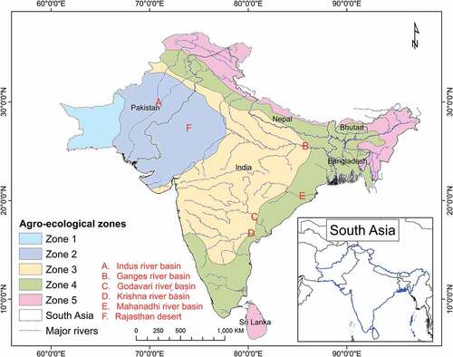
The original GAEZs were defined on the basis of a combination of soil properties and climatic characteristics. The specific parameters used in our definition were related to the climatic requirements for the crops and the management systems under which they are grown. Each AEZ thus delineated in this study had a similar combination of constraints and potentials for land use, and thus served to focus recommendations on improving the existing land-use situation, either through increasing production or by limiting land degradation.

2.1. Definitions

Definitions are key to mapping. In this study, we defined irrigated areas as all the cropland areas which get one or more water application during the growing/vegetative season from artificial sources other than precipitation. These irrigated areas include water from reservoirs by building dams of rivers, river water diversions through a barrage, pumping along the riverbanks, pumping from deep acquirers or shallow acquirers by digging tube wells or open wells, and irrigation tanks along the small order streams. The rainfed croplands are croplands that grow crops purely dependent on rainfall without any need for artificial water diversions.

3. Data

3.1. Remote sensing analysis-ready data (ARD) cube

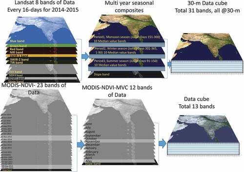
We have two separate ARDs (Figure 2). The top Figure 2 illustrates ARD for Landsat 30 m data, available as surface reflectance product on the GEE, used for the product: irrigated versus rainfed croplands. The bottom Figure 2 illustrates ARD for MODIS 250 m data, also available as surface reflectance product on the GEE, used for the products: cropping intensity and crop types.

Figure 2. Top row: For each of the five agro-ecological zones in South Asia, 16-day bands of Landsat-8 operational land imager (OLI) data (Miller 2016)were used to make multi-year composites of three cropping seasons (2013–2015). Overall, 10 bands including indices (blue, green, red, NIR, SWIR1, SWIR2, TIR, EVI, NDVI, NDWI) were time composited over every season to arrive at data cubes for each zone. Stacked 30 bands (3 seasons x 10 bands)) and one slope band, making it a total of 31 bands. Bottom row: To define cropping intensities and crop types, MODIS 250 m NDVI daily data (Modis 2022) were time composited into 23 bands with MOD13Q1.6 products. These were further composited into 12 bands of maximum-value composites (MVCs) to constitute analysis-ready data (ARD) and also stacked one slope band for this research.

3.1.1. Landsat data for irrigated and rainfed croplands

For irrigated versus rainfed croplands, our study drew upon multiple bands (Blue, Green, Red, Near Infrared (NIR), Short wave Infrared (SWIR1 & 2, Thermal Infrared (TIR)) as well as indices (Equation 1(1) $NDVI=\frac{\left(NIR-\mathrm{R}\mathrm{e}\mathrm{d}\right)\hspace{0.17em}}{\left(NIR+\mathrm{R}\mathrm{e}\mathrm{d}\right)}$(1) , 3(3) $EVI=\frac{2.5\ast (\left(NIR-Red\right)}{\left(\mathrm{N}\mathrm{I}\mathrm{R}+6\ast \mathrm{R}\mathrm{e}\mathrm{d}-7.5\ast \mathrm{B}\mathrm{l}\mathrm{u}\mathrm{e}+1\right)}$(3) and 4(4) $NDWI=\frac{\left(Green-\mathrm{N}\mathrm{I}\mathrm{R}\right)\hspace{0.17em}}{\left(Green+\mathrm{N}\mathrm{I}\mathrm{R}\right)}$(4) ) of Landsat-8 30 m data acquired every 16 days from 2013 to 2015. This resulted in 10 band composites for each of the 12 months composited over 3 years (2013–2015). This resulted in a total of 120 bands. Then, season-wise median values for each band (i.e. first season – Day 151 to 300 (rainy), second season – Day 301 to 365, 1 to 90 (winter), Third season – Day 91–150 (summer), which contains 10 bands for every season (30 bands for three seasons). In addition, a slope band (which helps in distinguishing cropland from other LULC) was added, for a total of 31 bands (top portion of Figure 2).

3.1.2. MODIS data for cropping intensity and crop type

For mapping of the cropping intensity and crop type, we used MOD13Q1.6 derived 250 m normalized difference vegetation indices (NDVI) data (Lpdaac 2016), which were time-composited for every 16-day interval (bottom image in Figure 2). The 16-day MODIS tiles covering the whole South Asian region for the duration of June 2014 to May 2015 were extracted from the Land Processes Distributed Active Archive Center (LP DAAC) (https://lpdaac.usgs.gov) (Lpdaac 2016). The MODIS re-projection tool i.e. MRT was used to re-project and mosaic all tiles and then stacking them as a single composite (Thenkabail et al. 2009; Gumma et al. 2011) (bottom image in Figure 2). The Normalized Difference Vegetation Index (NDVI) (Rouse et al. 1974) was derived from the near infrared and red band for 16-day composite in the 2014–2015 time series of images using equation 1(1) $NDVI=\frac{\left(NIR-\mathrm{R}\mathrm{e}\mathrm{d}\right)\hspace{0.17em}}{\left(NIR+\mathrm{R}\mathrm{e}\mathrm{d}\right)}$(1) :

(1) $NDVI=\frac{\left(NIR-\mathrm{R}\mathrm{e}\mathrm{d}\right)\hspace{0.17em}}{\left(NIR+\mathrm{R}\mathrm{e}\mathrm{d}\right)}$(1)

(2) $NDVIMV{C}_i=Max\left(NDV{I}_{i1},NDV{I}_{i2}\right)$(2)

(3) $EVI=\frac{2.5\ast (\left(NIR-Red\right)}{\left(\mathrm{N}\mathrm{I}\mathrm{R}+6\ast \mathrm{R}\mathrm{e}\mathrm{d}-7.5\ast \mathrm{B}\mathrm{l}\mathrm{u}\mathrm{e}+1\right)}$(3)

(4) $NDWI=\frac{\left(Green-\mathrm{N}\mathrm{I}\mathrm{R}\right)\hspace{0.17em}}{\left(Green+\mathrm{N}\mathrm{I}\mathrm{R}\right)}$(4)

where the MVC_i is the monthly maximum-value composite (MVC) of i^th month (e.g. “i” is June–May). i1, i2 are every 16-day composite image in a month (equation 2(2) $NDVIMV{C}_i=Max\left(NDV{I}_{i1},NDV{I}_{i2}\right)$(2) ). Altogether 23 images, each covering the entire study area of South Asia, were stacked. From the 16-day, monthly MVCs (i.e. maximum NDVI values for each month as per equation (1)(1) $NDVI=\frac{\left(NIR-\mathrm{R}\mathrm{e}\mathrm{d}\right)\hspace{0.17em}}{\left(NIR+\mathrm{R}\mathrm{e}\mathrm{d}\right)}$(1) were established and stacked for the crop year 2014–15 (June 2014 to May 2015). This gave us an analysis-ready data (ARD) cube (bottom image in Figure 2) of 12 MODIS NDVI MVCs (one for each month), thus providing wall-to-wall coverage of the whole of South Asia. A single-band of slope data was also stacked. Thus, the ARD data cube forms 13 bands for further processing (Figure 2, bottom row).

3.2. Reference (training and validation) data hub

Ground-level reference survey information was collected extensively by a very experienced survey team across South Asia for the crop year 2014–15 (June 2014 to May 2015) for the purposes of land class identification, labeling and accuracy assessment. Overall, there were 2,734 ground reference data samples of which 1,947 points were used for training reference data and 787 for validation (Table 1), for which the data repository is ICRISAT (ICRISAT 2022). The ground-level training data were used to create a knowledge base for training the machine learning algorithms like RF and for generating ideal spectral signatures for the SMTs. For each ground sample (which were at least 250 m x 250 m) LULC information was collected along with crop type, soil type, and irrigation type. At each data collection point, the area around was classified into one of three classes: small (≤10 ha of irrigated area present around the survey location), medium (10–15 ha), or large (≥15 ha). Whenever possible, farmers were interviewed for information on planting dates, irrigation type and cropping pattern. Other information was obtained from other sources too such as local agriculture experts and secondary sources such as reliable maps, where available, of local areas. The LULC names and class labels were assigned in the field using a labeling protocol (Thenkabail et al. 2009). Locations were measured by Global Positioning System (GPS) (3 m accuracy) and photographs were taken of crops grown. The ground data thus collected were further divided and refined as per the purposes of the study: delineation of irrigated vs. rainfed cropland (Figure 3), crop intensity pattern (Figure 4) and crop type\dominance (Figure 5). For crop intensity mapping, the ground data were categorized as per single, double, and triple cropping samples, which gave us 1098 training samples and 629 validation samples (Figure 4). As regards, the crop-type mapping, the ground data were categorized by major crop types and also season-wise, which yielded 851 samples for training and 858 samples for validation (Figure 5; Figure 6). The GPS location is a precise one (+ or – 3 m). These locations are carefully selected during field visits for each crop in large homogeneous fields. For example, a maize field GPS location is centered at the field surrounded by the same crop in all directions. Therefore, the ideal spectra generated for the center location is very much representative for the field irrespective of whether it is 250 m or 30 m.

Figure 3. The spatial extent of ground data (training and validation) data (ICRISAT 2022; Gumma et al. 2017) collected for mapping of irrigated and rainfed croplands (product 1) in South Asia.

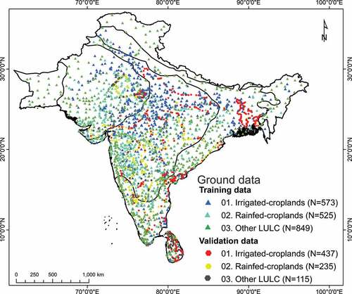
Figure 4. Spatial distribution of ground sample (training and validation) data ((ICRISAT 2022; Gumma et al. 2017) collected for mapping crop intensity (product 2) in South Asia using MODIS data Miller 2016)).

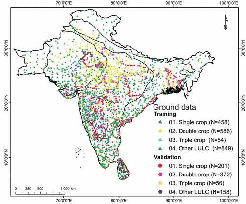
Figure 5. Spatial distribution of the ground reference (training and validation; ICRISAT 2022; Gumma et al. 2017) collected for mapping of major kharif crops (product 3) using MODIS 250 m data (Miller 2016).

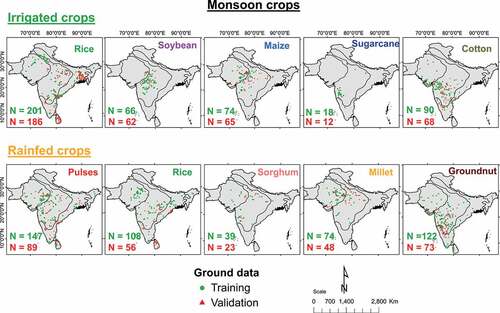
Figure 6. Spatial distribution of ground data (training and validation) data (ICRISAT 2022; Gumma et al. 2017) for mapping of major rabi crops (product 3) in South Asia using MODIS 250 m data (Miller 2016).

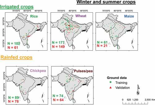
Table 1. Product-wise ground reference training and validation data samples collected for the whole of South Asia (ICRISAT 2022).

Cropland	Ground data
	Training samples	Validation samples
Irrigated vs. rainfed
Irrigated	573	437
Rainfed	525	235
Non-crop /other LULC	849	115
Crop intensity
Single crop	458	201
Double crop	586	372
Triple crop	54	56
Major crop type
Rice	201	230
Soybean	66	62
Maize	74	65
Groundnut	122	73
Pulses	147	89
Sugarcane	18	12
Potato	8	18
Millets	74	48
Chickpea	89	78
Cotton	90	68
Sorghum	39	23
Other crops	38	62

3.3. Statistical data

Statistical data are significant to compare cropland areas calculated within an administrative unit with those reported by national and local statistical agencies. For the purposes of this study, statistical data for India were acquired from the Directorate of Rice Development (http://dacnet.nic.in/rice/) (Ray, Singh, and Choudhary 2021) of the Ministry of Agriculture. Statistics for Bangladesh, Nepal, Pakistan, Nepal, and Bhutan were obtained from the respective national statistical departments (Aid 2021; Bbs 2021; Nsb 2021).

4. Methods

Our study was aimed at three remote-sensing products that capture important cropland characteristics across South Asia:

Product 1: Irrigated croplands versus rainfed croplands

Product 2: Crop types

Product 3: Cropping intensity

The methodology we followed is represented in Figure 7 and described below in subsections.

Figure 7. Methodology used for mapping three cropland products for the whole of South Asia. Product 1: Irrigated croplands versus rainfed croplands using landsat 8 data at 30 meters resolution in the google earth engine (GEE) interface. Products 2 and 3: Cropping intensity and crop type using MODIS 250 meters data on earth resources data analysis system (ERDAS) imagine.

4.1. Methods for product 1: mapping irrigated and rainfed cropland using RF machine learning algorithm

In making Product 1 to delineate irrigated croplands from rainfed croplands, we adopted the RF machine learning algorithm and computing was performed on the GEE cloud platform, which is equipped with hitherto unheard-of petabyte-scale big data analytics (Dubey et al. 2020). The RF machine learning algorithm is a pixel-based supervised classifier. The method involves the following steps:

4.1.1. Reference training data collection

The first step is to gather well-distributed reference training data. Figure 3 shows the training data used in developing irrigated versus rainfed cropland RF machine learning algorithm.

4.1.2. Knowledge base creation

Knowledge base creation for training of the RF machine learning algorithms involved obtaining Landsat 8 time-series signatures from the ARD (Figure 2, top half) utilizing the irrigated and rainfed cropland training datasets (Figure 3). The knowledge base is made robust to ensure that there is maximum separability of irrigated and rainfed cropland classes as shown in Figure 7A for AEZ 2 (Figure 1). Similar knowledgebases were created for other AEZs shown in Figure 1. There were instances where clear variability/separability was infeasible in some AEZ when the entire AEZ was taken into consideration. In such cases, we further divided AEZs into sub AEZs and created knowledgebase for clear and distinct separability between irrigated and rainfed crops in sub AEZs and then the product is put together over entire AEZ and finally over entire South Asia. Sub-AEZs were derived from AEZs (Figure 1) by using layers such as elevation, slope, climate (precipitation, temperature), and soils.

4.1.3. Running machine learning algorithms

The knowledge base created was used to run the RF machine learning algorithms (Rodriguez-Galiano et al. 2012; Xiong et al. 2017a) on the GEE cloud with multiyear seasonal data from Landsat-8 30 m ARD (e.g. top half of Figure 2) data cube to best separate irrigated areas from rainfed areas. The performance of the RF machine learning algorithms depends on the robustness of the reference training data as well as number of decision trees. A random forest (RF) is an ensemble classifier that generates a set of multiple decision trees and then votes for the most popular class, using a randomly selected subset of training samples and variables (Thenkabail et al. 2021). The RF uses hundreds of classifiers that are built into RF classification, and their decisions are combined, usually by plurality vote, using the premise that accuracy is greater from combining ensemble classifiers than it is from any single ensemble classifier, thereby avoiding conflicts among the feature subsets (Tian et al. 2016). The RF classifier uses bootstrap aggregating (bagging) to form an ensemble of decision trees by searching random subspaces from the given features and the best splitting of the nodes by minimizing the correlation between the decision trees (Xiong et al. 2017a). It provides a means of averaging predictions of multiple decision trees, trained on different subsets of the same data, in order to overcome the problem of overfitting by individual decision trees (Kranjčić et al. 2019; Shah et al. 2019). At the same time, the quality of samples and well-distributed samples are very important. The process is iterative, meaning that after each run the classification accuracies are assessed. The process is repeated by refining the training data and improving the knowledge base till a highly accurate irrigated versus rainfed cropland product is obtained. Refinement of the knowledge base involves dropping and adding reference training data that have high degree of uncertainty until it ultimately leads to an optimal solution that has optimal producer’s and user’s accuracies.

The process involved generating Landsat 8, 30 m analysis-ready data (ARD) cubes (Figure 2) for five AEZs in South Asia (Figure 1), generating a knowledge base for them, and running RF machine learning algorithms for each AEZ separately.

One of the best ways to separate irrigated croplands from rainfed croplands is through phenology. A large proportion of irrigated areas in South Asia have second and/or third crops over a 12-month period whereas rainfed areas almost always have only one crop coinciding with the rainy season. When, in spite of the above measure, significant issues of separability arise, other data are introduced in the data cube such as indices, slope, and thermal data (Dheeravath et al. 2010) to achieve optimum separation.

4.2. Method for product 2: crop type mapping using quantitative spectral matching technique

MODIS 250 m data were used to classify and identify crop types using quantitative spectral matching techniques (SMTs). The SMTs involved developing ideal spectral signatures (ISSs), classifying images and obtaining class spectral signatures (CSSs), and matching class spectra with ideal spectra to identify and label crop-type classes (Thenkabail et al. 2007). Methodological steps involve the following steps:

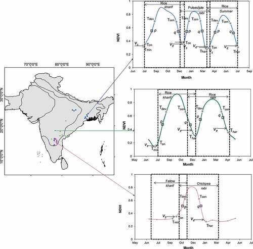
4.2.1. A. Ideal spectral signatures

Ideal spectral signatures were produced using MODIS NDVI time-series data with precise knowledge of croplands based on the unique reference samples obtained from the ground survey. The reference samples were classified according to their unique categories and grouped into homogeneous classes considering cropping intensity, crop types, and cropping system. Figure 8 shows the ideal spectral signatures of various crops, both irrigated and rainfed. The spectral signature curve explains crop behavior over time (Thenkabail et al. 2007; Gumma et al. 2016). During the initial stage of crop growth, it has a smaller NDVI value; during peak growth, the NDVI value is high; and at harvest stage, the NDVI value is again smaller (Figures 8 and 9). Given the precise knowledge of the crop type based on ground data, we have clear understanding of how each crop behaves in terms of NDVI over time (Figure 8). These ideal spectral signatures (ISSs) are derived for various crops in different AEZs or, if need be in sub AEZs.

Figure 8. Spectral signatures of major crops obtained using MODIS NDVI time-series data (sample size = 10) (Gumma et al. 2017; ICRISAT 2022).

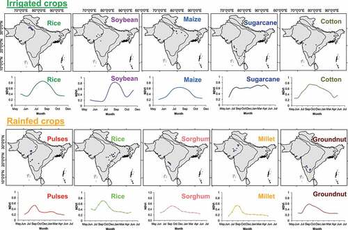
Figure 9. Spectral matching techniques (SMTs) to match class spectra with ideal spectra extracted from MODIS 250 m time series data (Gumma et al. 2017; ICRISAT 2022).

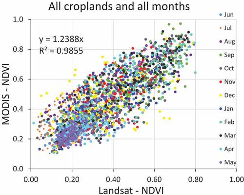
In order to generate ideal spectra across resolutions using the same samples, we selected crop-type samples in the middle of the field. These are representative homogeneous fields. So, the GPS location at the center of the field has the same crop in all 4 directions (at least 125 m in each direction), which makes the sample grid resolution at least 250 m x 250 m. That way, the samples can easily be used to develop ideal spectra for 30 m x 30 m Landsat or 250 m x250m MODIS or for other resolutions within 250 m x 250 m. Thereby, there is clear relationship between the MODIS and Landsat spectral reflectivity and NDVI (as shown in the Appendix 1). Indeed, MODIS NDVI were highly correlated with Landsat NDVI for crops with an R-square value of 0.74. The relationship equation was:

(5) $\mathrm{M}\mathrm{O}\mathrm{D}\mathrm{I}\mathrm{S}\mathrm{N}\mathrm{D}\mathrm{V}\mathrm{I}=1.0471\ast \mathrm{L}\mathrm{a}\mathrm{n}\mathrm{d}\mathrm{s}\mathrm{a}\mathrm{t}+0.0877$(5)

This strong relationship shows that same samples can be used for both sensors (or any other sensors as long as they are within 250 m x 250 m). Given the differences in sensor characteristics (e.g. spatial resolution, spectral bandwidth, radiometry) it is expected that they have a relationship with certain slope and intercept. When using multi-sensor data, this is a common approach to develop inter-sensor relationships and develop an understanding on how the spectral reflectivity and\or NDVI are related to one another

4.2.2. B. Class spectra generation

Class spectra were generated based on unsupervised classification of MODIS 250 m, 16-day NDVI time-series data for the year 2014–2015 using the ISOCLASS cluster algorithm (ISODATA in ERDAS Imagine 2021^TM, ERDAS Imagine, 2021 followed by progressive generalization (Cihlar et al. 1998). The initial classification was set at a maximum of 160 iterations and a convergence threshold of 0.99, which resulted in 160 classes for the whole of South Asia. Spectral signatures were generated for every individual class.

4.2.3. C. Matching of class spectra on the basis of ideal spectra to group classes using SMTs

The process of SMT mainly involves two steps:

(i) Grouping similar class spectra: The initial 160 classes obtained from unsupervised classification (called class spectra) were grouped into a subgroup based on quantitative spectral matching techniques (QSMTs), i.e. classes nearly similar spectral profiles (Homayouni and Roux 2003; Thenkabail et al. 2007) (see Figure 9, middle column). For example, a group of 10 classes having similar MODIS NDVI time-series temporal spectral signatures are nearly matched with ideal spectra (Figure 9, middle column (ICRISAT 2022).

(ii) Matching group of similar classes with ideal spectra. Spectral matching involves, finding an ideal spectra that matches with group of class spectra (Figure 9). This is achieved by group of quantitative spectral matching techniques (QSMTs) methods such as spectral correlation similarity (SCS) R-square values between the ideal spectra and class spectra. When an R-square value of 0.80 or higher is achieved in correlation between ideal spectra and class spectra then it is considered as a match. In Figure 9 we see visual matches both in terms of their shape and magnitude in the time-series NDVI spectra of ideal spectra and class spectra for three cases. Once such strong relationships are identified between a group of class spectra with an ideal spectrum, then a preliminary class name is assigned taking the name of ideal spectra. This preliminary labeling of classes is further validated mainly by using ground data for all the classes in the group, use of very high-resolution imagery, and data from ancillary sources such as available maps. The same process is repeated in identifying and labeling all 160 classes, leading to final classes. Some classes may not match with the spectral signatures. These classes were masked out and re-classified using the above protocols (Thenkabail et al. 2007; Gumma et al. 2011, 2014). By combining all similar classes, a crop type and\or crop dominance map was produced.

Classifications for categorizing crop types were conducted separately using irrigated and rainfed masks (section 4.1) and then the classes identified using the separate knowledgebase for irrigated areas (Figure 8) and rainfed areas (Figure 9) using the QSMTs described in this section.

4.3. Method for Product 3: Cropping intensity map

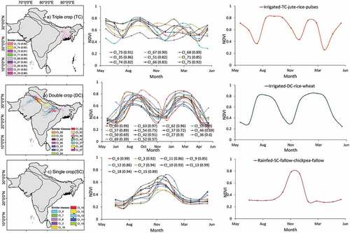
Cropping intensity was mapped with the help of spectral signatures that involved time-series NDVI profiles (Figure 10).

Figure 10. Spectral signatures obtained using MODIS derived NDVI time series data showing crop intensity in South Asia. Temporal NDVI profile and transition dates for three crop seasons are shown. Each peak indicates a crop season (Note: sample size = 10) (Gumma et al. 2017; ICRISAT 2022).

Cropping intensity was identified by analyzing the peaks of the temporal NDVI profiles of the classes obtained during the unsupervised classification. In Figure 10, the curve with three peaks indicates triple cropping (e.g. Irrigated-TC-pulses/rice-rice) in a crop year. The double crop (DC) (e.g. irrigated-DC-rice-wheat, irrigated-DC-rice-rice) classes contain two peaks in a single curve, with the first peak indicating a crop in the first season and the second peak representing a second crop in the later season. In the third graph, there is only a single peak, which means there was only a single crop (SC) (e.g. rainfed-SC- rice-fallow, rainfed-SC-sorghum etc.) in that crop year. The crop intensity algorithm was thus applied to each of the five AEZs studied for identification of single, double and triple cropping. Arid regions have mainly single cropping whereas semi-arid and humid regions contain double or tiple cropping depending on irrigation facility.

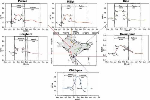
Figure 11 shows the vegetation phenology and transition dates for various irrigated crops, mainly rice-wheat (i.e. rice during kharif followed by wheat during Rabi), soybean-wheat, maize-wheat, sugarcane, rice-rice, and cotton. Note that sugarcane and cotton cut across seasons. Figure 12 shows rainfed crops, mainly pulses, millet, rice, sorghum, groundnut and chickpea. Rainfed crops illustrated in Figure 12 have only one crop annually (which is the case overwhelmingly). In both figures, T_min denotes the beginning of the time series, Ton is onset of greenness, T_dev is the beginning of the development stage, T_sen the onset of senescence, and T_har harvesting time. p and q are the inflection points. There are several distinctive features that distinguish irrigated crops (Figure 11) from rainfed crops (Figure 9). First, irrigated crops are often double crops (two crops annually). Rainfed crops are overwhelmingly single crops (one crop annually). Second, irrigated crops and rainfed crops follow their own phenological cycles. Irrigated crops have more clear firm cropping calendars whereas rainfed crops depend on rainfall events. The magnitude of NDVI for most irrigated crops are higher. All this knowledge is used in the knowledge base created for training of the RF machine learning algorithm and to classify Landsat image data cubes (e.g. top half of Figure 2).

Figure 11. Spectral signatures obtained using MODIS derived NDVI data showing vegetation phenology and transition dates for irrigated crops during the kharif season. Map also shows the ground samples and ideal signatures of various crops (Note: sample size = 10) (ICRISAT 2022; Gumma et al. 2017).

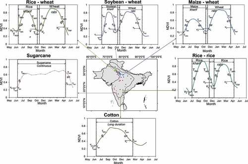
Figure 12. Spectral signatures obtained using MODIS derived NDVI data showing vegetation phenology and transition dates for rainfed crops during the kharif/rabi season. Map also shows the ground samples and ideal signatures of various crops (Note: sample size = 10) (ICRISAT 2022; Gumma et al. 2017).

4.4. Accuracy assessment

Accuracy assessment was based on a total of 786 independent ground survey sample points that were not used in the class identification and labeling process. Accuracies were obtained using error matrices (Congalton 1991) and established for all the three crop products included in this study. The overall accuracies, producer’s accuracies (or errors of omission) and user’s accuracies (or errors of commission) were obtained for all classes in the respective cropland products.

5. Results

The results are documented and discussed for each of the three cropland products.

5.1. Product 1: irrigated versus rainfed croplands

The spatial distribution map of irrigated and rainfed croplands of South Asia derived using Landsat 30 m data is shown in Figure 13. There is a total of 228.6 million hectares of croplands in South Asia of which 55% is irrigated (126.4 Mha) and 45% is rainfed (102.2 Mha) (Table 2, Figure 13). Most of the irrigated croplands are located below the Himalayan Mountain ranges dominated by the Ganges and the Indus river basins as well as by the major river basins throughout South Asia (see Figure 1 for locations). These river basins provide irrigated water through reservoirs created by dams, run of the river diversions through barrages, and riverine water through flows throughout the years either due to runoff from rainfall or from snowmelt from Himalayan rivers. Major sources of water for irrigation also come from ground water (wells on deep acquirers and shallow acquirers), and tanks or small reservoirs along the low-order streams. Rainfed crops are found in some concentration in Rajasthan and Odisha states of India and in parts of southern and northeastern India.

Figure 13. The Landsat derived irrigated versus rainfed cropland map of South Asia (2014–15). The map was made using 30 m time-series data from Landsat 8 on the Google Earth Engine (GEE) platform.

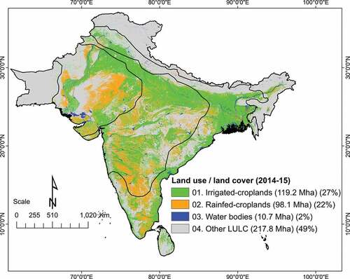
Table 2. Irrigated and rainfed cropland (Product 1) cropping intensity (Product 3) in South Asia in 2014–15.

Product 1: Irrigated vs rainfed croplands (30 m)
LULC #	Area (‘000 ha)	TNCA* (%)
1. Irrigated cropland	119,235	55%
2. Rainfed cropland	98,144	45%
3. Other LULC	228,619	NA
Product 3: Crop intensity (250 m)
LULC #	Area (‘000 ha)	TNCA* (%)
1. Single cropping	92,365	41%
2. Double cropping	126,344	55%
3. Triple cropping	9,861	4%
4. Other LULC	217,746	NA

*TNCA = Total net cropped area. Note: Product 2 (crop type\dominance) is not presented here since there are many crops, but their areas presented in Figures 14 and 15.

5.2. Product 2: crop type\dominance

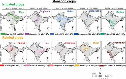
Figure 14 shows the spatial extent of the five irrigated crops (rice, soybean, maize, sugarcane and cotton) and five rainfed crops (pulses, rice, millet, sorghum, and groundnut). This distribution shows crop dominance in various regions of South Asia. In the monsoon (rainy) season, most of the irrigated rice areas (Figure 14A) are concentrated in the northern part of South Asia and along the rivers, amounting to almost 16% of the total cropped area. Irrigated soybean (Figure 14B) is seen mostly in Madhya Pradesh state of India, occupying about 6% of the total cropped area. Irrigated maize (Figure 14C) is found across south Asia, accounting for about 8% of the total cropped area. Irrigated sugarcane (Figure 14D) with 2% of the cropped area is mostly located in north India whereas most of the irrigated cotton (Figure 14E), with 11% of total cropped area, is found in the southern part of South Asia. In the dry areas, most of the crops sown during the monsoon season are dependent on rainfall: pulses (Figure 14F) grown on rainfed cropland are concentrated in the western part of South Asia with almost 13% of the total cropped area; and rainfed rice (Figure 14G) is found in the eastern part of south Asia with almost 11% of the total cropped area. Sorghum (Figure 14H) and Millet (Figure 14I) take a significant share (about 11%) of the rainfed area in South Asia whereas rainfed groundnut area (Figure 14J) is located in the southern part of South Asia with almost 3% of the total cropped area.

Figure 14. Spatial distribution of crop extent on irrigated and rainfed croplands in South Asia during the kharif (monsoon) season of 2014–15. The mapping was done using MODIS time-series data (Modis 2022). The 8 crops named above occupy 184 Mha (80.4% of the net cropped area) during the kharif season.

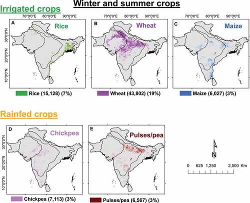
As most of the cropland in south Asia has double intensity, crops are grown in winter and summer seasons (Figure 15), with crops like rice (Figure 15A), wheat (Figure 15B), and maize (Figure 15C) being cultivated with the help of irrigation facilities. The share of irrigated rice is about 7% of the total cropped area while irrigated maize takes almost 3%. The largest share of the total cropland area is taken by wheat, nearly 19%, mostly in north India. There are a few rainfed crops like chickpea (Figure 15D) and pulses (Figure 15E) that are sown in the winter and summer seasons, relying on the residual moisture in the field as well as atmospheric moisture, with almost 6% of the total cropped area.

Figure 15. Season-wise crop type map, made by using MODIS time-series data (Modis 2022), showing cropped area and percentage of total cropped area for South Asia for the rabi season, 2014–15. The five crops shown above occupy 78.63 Mha or 34.4% of the total net cropped area.

5.3. Product 3: cropping intensity

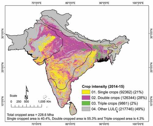
Crop intensity in South Asia mainly depends upon water availability, either from rainfall or from irrigation, during the cropping seasons. Irrigated croplands allow double or triple cropping annually (in a 12-month period) whereas rainfed croplands are almost always limited to single crops due to rainfall events such as the South-West Monsoon (June–September) or Northeast Monsoon (October–December). The map in Figure 16 shows that of the 228.6 Mha of croplands in South Asia, 40.4% is in single crop, 55.3% double crop, and 4.3% triple crop. Single crop is mainly rainfed, double and triple crop is overwhelmingly irrigated. There are also significant irrigated areas in single crop. Triple crop is almost all is Bangladesh or NE India. Double crop is in Indus and Ganges River basins and along other major rivers such as Mahanadhi and Krishna and Godavari. Rainfed areas are dominant in the Deccan Plateau and in the Rajasthan desert fringes.

Figure 16. Cropping intensity map of South Asia (2014–15) produced by using MODIS 250 m NDVI time-series data.

5.4. Accuracy assessment

Accuracy assessment was mainly carried out for cropland classification, cropland intensity and crop water methods and for cropland versus non-cropland comparison. The irrigated and rainfed croplands of South Asia were mapped with an overall accuracy of 79.8% (Table 3). The producer’s accuracies of the irrigated crops (Figure 13) were 79% (errors of omissions 21%) (Table 3) and that of rainfed crops was 74% (errors of omissions 26%) (Table 3). The user’s accuracies of the irrigated crops (Figure 13) were 87% (errors of commissions 23%) (Table 3) and that of rainfed crops was 63% (errors of commissions 37%) (Table 3). A producer’s accuracy of 79% for irrigated crops means that 79% of the irrigated areas are actually mapped as irrigated areas. By corollary 21% of irrigated areas were not mapped as irrigated areas (errors of omissions). A user’s accuracy of 74% for irrigated crops indicates that there in 26% non-irrigated areas captured as irrigated (errors of commissions). The similar interpretations for rainfed croplands (Table 3). These are very good results comparable to several other studies in mapping irrigated and rainfed croplands using remote sensing (Siebert et al. 2007; Dheeravath et al. 2010; Sarmah et al. 2021). Dheeravath et al. (2010) identified irrigated croplands and achieved 83% accuracy whereas our study achieved 87% accuracy of irrigated area and other studies Siebert et al. (2007) mapped irrigated at very low resolution (10 km and 1 km).

Table 3. Accuracy assessment using the error matrix method with field-plot data for irrigated croplands, rainfed cropland and other LULC classes.

Land use/land cover	Irrigated cropland	Rainfed cropland	Non-croplands (Other LULC)	Producer’s accuracy	User’s accuracy	Error of omission	Error of commission	Kappa
Irrigated croplands	369	45	6	79%	87%	21%	13%	66%
Rainfed croplands	84	146	0	74%	63%	26%	37%	51%
Noncroplands (Other LULC)	13	5	89	94%	83%	6%	17%	81%
Total (no.)	466	196	95
Overall classification accuracy = 79.8%					Overall Kappa statistics = 0.630

(Note: Field plot data are on X-axis/row and MODIS classification on Y-axis/column). Note: kappa statistic is defined in Congalton and Green, 2019).

The overall accuracies of mapping cropping intensity (single, double, and triple cropping; Figure 16) was 85.3% (Table 4). The producer’s accuracies were 88% for the single crops, 85% for the double crop, and 67% for the triple crop (Table 4). The user’s accuracies were 86% for the single crops, 92% for the double crop, and 72% for the triple crop (Table 4). Overall, the cropping intensity was mapped with excellent results. The triple cropping is slightly difficult with often the class mixing with the double crop. Since the triple crop has much less area (Figure 16) relative to the other two crops the impact on the uncertainties in accuracies is mostly reflected for this class.

Table 4. Accuracy assessment using the error matrix method with field-plot data for the cropping intensity product.

Land use/land cover	Single crop	Double crop	Triple crop	Other LULC	Producer’s accuracy	Users accuracy	Error of omission	Error of commission	Kappa
Single crop	170	27	1	0	88%	86%	12%	14%	81%
Double crop	14	349	9	8	85%	92%	16%	8%	82%
Triple crop	0	13	33	0	67%	72%	33%	28%	70%
Other LULC	10	24	6	99	93%	71%	7%	29%	67%
Total (no.)	194	413	49	107
Overall classification accuracy = 85.3%				Overall Kappa statistics = 0.77

(Note: Field plot data are on X-axis/row and MODIS classification on Y-axis/column). Note: kappa is defined (Congalton and Green 2019).

Crop types (Figures 14 and 15) were mapped with high degree of confidence during the monsoon (main) cropping season, as well as during the rabi\winter season (Table 5). For the irrigated crops (rice, soybeans, maize, sugarcane, and cotton) the accuracies varied between 83% and 94%. During the Monsoon season, the rainfed crops (Pulses, rice, sorghum, millets, and groundnut) were mapped with accuracies varying between 70% and 81%. During the second crop of Rabi\winter, the three irrigated crops (rice, wheat, maize) were mapped with an accuracy of 82–97%. In the same season, the two rainfed crops (Chickpea and pulses) were mapped with an accuracy of 78–87%. Crop types were, generally, mapped with high degree of confidence given the focus was on major crops and in clearly dominant crop growing regions in given seasons. With good set of reference data applied on multi-date remote-sensing crop types were captured with very good accuracies.

Table 5. Accuracy assessment using field-plot data using error matrix method (Congalton and Green 2019) for croplands product.

Season	Irrigated/Rainfed	Crops	No. of validation samples	Correctly classified pixels	Percent accuracy classifies
Kharif season	Irrigated crops	Rice	257	241	94%
		Soybean	41	38	93%
		Maize	36	26	72%
		Sugarcane	25	23	92%
		Cotton	72	60	83%
	Rainfed crops	Pulses	62	49	79%
		Rice	100	70	70%
		Sorghum	16	13	81%
		Millets	32	23	72%
		Groundnut	20	16	80%
Rabi season	Irrigated crops	Rice	166	161	97%
		Wheat	137	113	82%
		Maize	16	14	88%
	Rainfed crops	Chickpea	37	29	78%
		Pulses/pea	46	40	87%

(Note: X-axis/row is Field plot data and Y-axis/column is MODIS classification)

Nevertheless, the causes for errors of omissions and commissions in mapping various cropland products include limitations of the remote sensing data resulting in mixing of signatures across classes, failure to obtain reference data from certain types of irrigation or rainfed croplands leading to uncertainties in machine learning algorithms, and the host of other factors involved in complex mapping over very large areas (Thenkabail et al. 2021).

5.5. Comparison of remote sensing-derived crop area statistics with national statistics

The crop-type statistics derived from this study were compared with the crop-type statistics obtained from traditional National statistics (obtained by personal communication with the first author) as shown in Figure 17. For major crops like rice, wheat, soybeans, cotton, sugarcane, and chickpea the areas derived in this study explained 82–98% variability relative to the National statistics and the root mean square error (RMSE) varied from 0.2 Mha to 1.15 Mha (Figure 17). This clearly emphasizes the ability of MODIS 250 m time-series remote sensing data to accurately derive crop-type areas. However, maize, groundnut and sorghum areas derived from remote sensing explained only 60–65% variability in National statistics and the root mean square error (RMSE) varied from 0.29 Mha to 0.66 Mha. In the case of groundnut and sorghum, there is wide range of variability in crop growth characteristics of these two rainfed crop depending on the rainfall variability. All irrigated crops, except maize explained over 80% variability. Irrigated maize, however, explained only 60% variability. This is mainly due to large areal extent of maize crop which is spread across South Asia (Figure 14C). All other crops have dominance in certain regions of South Asia (Figure 14 A-B, 14-D-J), making them more stable in classification results. This implied that corn crop is better classified using more regional focus than performed in this study. Overall, it can be stated that irrigated crops are mapped with significantly higher accuracies than rainfed crops (Table 5), resulting in significantly better correlation of irrigated areas derived from remote sensing with the National statistics than with rainfed areas derived from remote sensing with National statistics (Figure 17). What is important to note here is that the slopes of the equations of areas of irrigated crops were close to 1 indicated excellent match with irrigated areas reported in the National statistics. However, for the rainfed crops the slopes differed significantly between the areas calculated by us when compared with areas calculated by the National statistics. This is to be expected given the wide variability in rainfed cropland systems across South Asia. Some rainfed crops are in high rainfed areas and other in driest areas.

Figure17. Comparison of remote sensing-derived crop areas with national statistics (ICRISAT 2022; Gumma et al. 2017).

The Figure 18 shows the comparison of district level irrigated area statistics with satellite derived irrigated area statistics. In India, there is an availability of irrigated area statistics for majority of districts, but there are some gaps in statistics of other countries. We have gathered irrigated data from various sources in respective countries like national agriculture websites and FAO. For India, about 92% was correlated and some districts, there is no availability of data. In other countries, Pakistan, Bangladesh, Nepal and Sri Lanka, the available district level irrigated statistics was significantly correlated above 90% with satellite-derived statistics.

Figure18. Comparison of remote sensing-derived irrigated areas with national statistics. District wise irrigated area statistics were obtained from national agriculture statistics of respective countries and food and agriculture organization (FAO) of the United Nations.

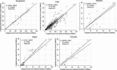
There is good correlation with the statistics obtained, even though there are some over and underestimates.

5.6. Comparison with various cropland products

We have compared our work with irrigated and rainfed cropland products from other sources, mapped using remote sensing at various resolutions. There are many studies at command area and lower administrative level on irrigated area mapping, but not to large extent like South Asia at 30 m resolution. The accuracies of such studies vary from 60% to 85%. Dheeravath et al. (2010) mapped irrigated and rainfed croplands of South Asia using MODIS 500 m time-series data (Modis 2022) with an overall accuracy of 83%. This product used the base map of the Central Board of Irrigation and Power (India) (Dheeravath et al. 2010) as baseline starting point. Thenkabail et al. (2009) and Biradar et al. (2009) mapped global irrigated and rainfed croplands at nominal 1 km using multi sensor remote sensing. This had an overall accuracy of 79% (Table 6). Siebert et al. (Siebert et al. 2007, 2015) produced global irrigated area map, that includes South Asia, using National statistics and GIS techniques at 1 degree resolution. Since all of these products (Table 6) are in 250 m to 1 km nominal resolution, there are a number of significant differences with the 30 m product produced here. First as a result of resolution differences of these products: 1 degree (111 km x 111 km), 1 km (1 pixel = 100 hectares), 500 m (25 hectares), and 30 m (0.09 hectares) does not allow direct comparison (Thenkabail et al. 2021). The 30 m product provides far greater details by capturing precise boundaries of croplands as well as in capturing the fragmented croplands. The coarser resolution products, often, provides crop dominance in a pixel or various percentage of croplands within a pixel. For example, the UN Food and Agricultural organization’s (UN FAO’s, Siebert et al. 2013)provides irrigated croplands as percent within a pixel (e.g. a pixel maybe 10% irrigated or 100% irrigated; it is scaled 1–100%) whereas in a 30 m pixel it is binary (e.g. every pixel is irrigated or non-irrigated). Similarly, for rainfed pixels. Further, the areas calculated from the coarser resolution products rely on sub-pixel areas (SPAs) as actual areas as every pixel area is multiplied by the fraction of irrigated or rainfed crop present within the pixel whereas in a 30 m pixel full pixel area (FPAs) are actual areas. Given these facts, obviously, the 30 m product represents greater precision in capturing irrigated and rainfed croplands.

Table 6. Various cropland extent products and their specifications(Biradar et al. 2009; Thenkabail et al. 2009; Velpuri et al. 2009; Dheeravath et al. 2010).

Number	Product	Spatial resolution	Year	Satellite data	Accuracy (%)
1	Irrigated Areas of India derived	500 m	2001–03	MODIS	83
2	Global irrigated area map (GIAM)	10 km	1992–93	AVHRR	79
3	Mapping Asian Cropping Intensity	500 m	2009–12	MODIS	~ 61

The accuracies seem to be higher for coarser-resolution imagery was due to the very large size of the pixel in coarser-resolution satellites (Velpuri et al. 2009).

There exist limited papers on crop intensity (Table 6). But at the large scale, only one paper mapped crop intensity at the Asia level (Gray et al. 2014) at 500 m resolution with an accuracy of 61% with limited ground data (only Bangladesh). We have mapped crop intensity at 250 m resolution with an accuracy of 85% with large ground data (Figure 16).

There are many crop-type maps available for small areas like command area and lower administrative levels, but our study mapped major crop types (12 crops) of South Asia for entire season (both kharif and rabi) with greater than 70% accuracy in each class, which is a unique product. Shukla et al. 2017 mapped rabi crop types (wheat, mustard, gram, masoor and potato) for Faizabad area and achieved an accuracy of 89% whereas (Wang et al 2020) did crop type (rice and cotton) for southeast India with 75% accuracy and (Yan and Ryu et al 2021) mapped crop type (8 crops) for California and achieved around 92% accuracy. Gumma et al., 2020 mapped crop type during rabi season for three districts (Jhansi, Chitrakoot and Panna) using sentinel −2 imagery and reported 84% of accuracy. Our results were in line with above studies in terms of accuracy.

6. Discussions

There are many cropland products mapped by numerous researchers (Siebert et al. 2007; Biradar et al. 2009; Pittman et al. 2010; Thenkabail et al. 2011; Fritz et al. 2015; Teluguntla et al. 2015; Eigenbrod et al. 2020; Hu et al. 2020) over the years using multiple-satellite sensor data and over diverse areas of the world. This study is unique in the sense it mapped three distinct cropland products: 1. Irrigated versus rainfed croplands using Landsat 30 m, 2. Crop types using MODIS 250 m data, and 3. Cropping intensities using MODIS 250 m data. Products were developed over entire South Asia, a heterogeneous landscape with a diversity of cropping patterns and several other LULC categories. Strength of the study was the availability of rich sets of ground data for training machine learning or other algorithms and validating the resulting cropland products. The value of multiple cropland products in global food and water security cannot be over emphasized (Thenkabail et al. 2021).

The cropland extent product was produced using Landsat 30 m data. The irrigated and rainfed areas within the cropland extent product were separated using Landsat 30 m data. Availability of irrigated and rainfed product helps in study of crops grown in these watering methods. This is of great importance for a number of reasons. First, crop productivity of irrigated areas is far more than rainfed areas. Second, the water uses in irrigated areas (blue water use) and rainfed areas (green water use) (Rost et al. 2008) helps accurate water accounting. Third, separating irrigated and rainfed croplands helps us in measures such as in planning sustainable food security for growing populations by understanding and strategizing productivity of lands, pinpointing areas for increase in productivity, and studying opportunities to expand irrigation to non-irrigated (rainfed) areas. Overall, irrigated and rainfed croplands were separated with good degree of separability. The factors that contribute to this separability includes: 1. Time composited Landsat 30 m OLI data over the years, 2. Rich ground data available to train machine learning algorithms, 3. Distinct cropping calendars of irrigated and rainfed areas, 4. Availability of base maps from the National systems that provide first level of irrigation command areas, 5. Ability to verify the products by comparing with National products, 6. Significantly greater magnitude of biomass produced (reflected in greater NDVI over time-series) in irrigated areas as opposed to rainfed areas, 7. Several other factors such as rich validation data, understanding of the regions agricultural crops and their dynamics by working in the field over the years, and 8. Adopting agroecological zones (AEZs) and sub AEZs in classifying and mapping irrigated areas. All these factors help identify label classes properly into distinct groups.

Cropping intensities were better mapped by MODIS 250 m data. This is because, MODIS 250 m data is acquired daily and composited into 16-day composites to overcome cloud and haze issues. In contrast Landsat 30 m data is acquired 8\16 days and can cause significant issues in studying cropping intensities due to cloud and haze issues in parts of the image. Further, the coverage of Landsat over the entire world is not as consistent as that of MODIS. That issue is overcome for the irrigated and rainfed product by filling gaps from nearby years as irrigated and rainfed areas do not change over short time periods. Cropping intensity, in contrast, need to be mapped for the year in consideration and data from other years will cause confusion and noise. MODIS 250 m NDVI time series provides a clear cropping phenology within and across seasons. So, one can identify through time series NDVI profiles whether a pixel is cropped once (single crop), twice (double crop), thrice (triple crop) or continuous (plantation crops that exist all through the year) in a 12-month period or annually. Cropping intensities of single and double crops are mapped with great confidence. The variability in mapping triple crop is relatively high as significant portions of this gets mixed with double crops. These results were in line with several other studies (Gray et al. 2014; Liu et al. 2020; Waha et al. 2020a; Li et al. 2021; Rufin et al. 2021).

Cropping intensity is rarely mapped over large areas within South Asia. Gray et al. (2014) mapped cropping intensity for Asia using MODIS 500 m data but had ground data limited to Bangladesh. Overall accuracy of this product was 61%. Gumma et al. (2014) mapped cropping intensity for Bangladesh at MODIS 250 m data at overall accuracy of 83%. This study mapped cropping intensities with overall accuracies of 85%. Cropping intensity mapping is very crucial as further cropland expansion in the world to meet global food security will come not from cropland expansion but from increasing cropping intensities (Thenkabail et al. 2021). Indeed, Global cropland intensification exceeded cropland expansion, first-time history, between 2010 and 2020 (Hu et al. 2020).

Crop types are best mapped by studying crops within the irrigated and rainfed areas. Crops in irrigated areas are distinct from crops in rainfed areas either in terms of crop types and\or crop characteristics like their biomass and other biophysical and biochemical characteristics. These differences are reflected in the NDVI magnitude over time and space for every pixel. By understanding and capturing these characteristics in an algorithm, crop types are mapped quite precisely, especially in the irrigated areas where the crop characteristics have greater stability over time and space. In rainfed areas, crop characteristics can show great degree of variability, especially when the rainfall timing and patterns vary over space and time. Thereby, in this study we showed high degree of confidence in mapping irrigated areas whereas the rainfed crops had greater degree of variability. These results were in line with some other studies (Shukla et al. 2017; Wang et al. 2020; Yan and Ryu 2021).

There are many crop-type maps available for small areas for various parts of the world including South Asia, but none for such large areas as South Asia; especially like this study that considers 12 major crops for rainfed and irrigated and over two main growing seasons (Khariff and Rabi). (Shukla et al. 2017) mapped rabi crop types (wheat, mustard, gram, masoor and potato) for the Faizabad area and achieved an accuracy of 89% whereas (Wang et al 2020) did crop types (rice and cotton) for southeast India with 75% accuracy and (Yan and Ryu et al 2021) mapped crop type (8 crops) for California and achieved around 92% accuracy. (Gumma et al., 2022) mapped crop type during rabi season for three districts (Jhansi, Chitrakoot and Panna) using sentinel −2 imagery and reported 84% of accuracy (Gumma et al. 2022). Our results were in line with the above studies in terms of accuracy. This study obtained crop-type accuracies of 70–97% for various crops (Table 5). The methods used in the study especially SMT can be transferred up to some extent, as the methodology depends mainly on the spectral signatures.

7. Conclusions

This study developed three distinct cropland products of South Asia for the year 2014–2015 in support of food and water security assessments and management. These three cropland products were:

1. Irrigated croplands versus rainfed croplands using Landsat 30 m data;

2. Crop types using MODIS 250 m data; and

3. Cropping intensity mapping using MODIS 250 m data.

Time-series Landsat 30 m and MODIS 250 m analysis-ready data (ARD) cubes were developed and analyzed. The methods used employed machine-learning algorithms to identify irrigated and rainfed cropland areas, cropping intensities using phenological matrices, and crop types using quantitative spectral matching techniques (SMTs). The computations were performed on the GEE cloud platform for the first product and on the workstations for the other two products.

The study established that the irrigated area in the whole of South Asia was 126.4 Mha (55% of the total net cropland area or TNCA); rainfed areas amounted to 102.2 Mha (45% of TNCA). The irrigated versus rainfed 30 m product has an overall accuracy of 79.8% with the irrigated class providing a producer’s accuracy of 79% (error of omissions of 21%) and rainfed cropland attaining a producer’s accuracy of 74% (errors of omissions of 26%). Single, double, and triple cropping percentages were, respectively, 40.4% (92.4 Mha), 55.3% (12.6 Mha) and 4.3% (9.9 Mha) of TNCA. The overall accuracy of the cropping intensity product was found to be 85.3% with producer’s accuracies of single, double, and triple crops at 88%, 85% and 67% respectively. Single and double crops were mapped with 85% or higher accuracy. The triple crops are only 4.3% of the overall croplands and significantly mixes with double crop and hence there is greater degree of uncertainty in mapping triple crops. For the kharif season (Jun-Oct), the main growing season, 10 major crops (5 irrigated crops: rice, soybean, maize, sugarcane, cotton; 5 rainfed crops: pulses, rice, sorghum, millet, groundnut) were mapped. Together they occupied 184 Mha (80.4% of TNCA): 99.2 Mha (54%) for the 5 irrigated crops and 84.8 Mha (46%) for the 5 rainfed crops. For the rabi season (Nov-Feb), the second season, 5 major crops (three irrigated crops: rice, wheat, maize; two rainfed crops: chickpea, pulses) were mapped. Together they occupied 78.6 Mha (34.4% of TNCA). Of this, 64.93 Mha (83%) were irrigated areas and 13.67 Mha (17%) rainfed. Crop types were mapped with accuracies ranging from 72% to 97%. The remote-sensing-derived crop type data explained 63–98% variability in the national statistics. Crop types were, generally, mapped with high degree of confidence, especially for irrigated crops where 80% or higher accuracies were achieved. Rainfed crops have higher uncertainty due to rainfall variability across large areas.

Highlights

• Multiple cropland products for South Asia were produced in support of food and water security.

• Distinct products include: (1) Irrigated versus rainfed cropland product at Landsat 30 m resolution; (2) cropping intensity at 250 m; and (3) crop type at 250 m.

• The overall accuracies of products were as follows: 79% for the irrigated versus rainfed cropland, 85% for the cropping intensity, and 72–97% for the crop type.

• Machine learning and GEE cloud computing and Spectral Matching Techniques (SMT’s) were used to develop the products.

Acknowledgements

This research was supported by The National Aeronautics and Space Administration (NASA) MEaSUREs (Making Earth System Data Records for Use in Research Environments) Program, through the NASA Research Opportunities in Space and Earth Sciences (ROSES) solicitation, and funded for a period of 5 years (1 June 2013–31 May 2018) and the Consultative Group for International Agricultural Research (CGIAR) Research Program Water, Land and Ecosystems (WLE), the CGIAR Research Program Climate Change, Agriculture and Food Security (CCAFS). We are grateful for the funding provided by the National Land Imaging (NLI) Program, Land Change Science (LCS) program, and the Core Science Systems (CSS) of the United States Geological Survey (USGS). Some of the research was conducted in the science facilities of the USGS Western Geographic Science Center (WGSC). We would like to thank to Dr Sunil Dubey, Assistant director, Mahalanobis National Crop Forecast Centre (MNCFC) for providing sub-national statistics from his Institute’s database. We would like to thank Dr Anthony Whitbread and Mr Irshad Mohammed for comments and their support. Any use of trade, firm, or product names is for descriptive purposes only and does not imply endorsement by the U.S. Government.

Data availability statement

All data pertaining to this research will be made available on the public domain in the The International Crops Research Institute for the Semi-Arid Tropics (ICRISAT) data portal (http://maps.icrisat.org/). In addition, other global food security-support analysis data (GFSAD) project data pertaining to South Asia are published by U. S. Geological Survey in The National Aeronautics and Space Administration’s (NASA’s) The Land Processes Distributed Active Archive Center (LP DAAC) (https://lpdaac.usgs.gov/products/gfsad30saafgircev001/) in (Gumma et al., 2017) and in (ICRISAT, 2022). These data include reference ground data used for training and validation as well as the cropland products presented in this paper. The cropland products released for the public include irrigated and rainfed, cropping intensities, and crop types.

Disclosure statement

No potential conflict of interest was reported by the author(s).

Additional information

Funding

This work was supported by the U.S. Geological Survey [This funding was received through NASA MEaSUREs project grant number NNH13AV82I and U.S. Geological Survey (USGS) sales order number 29039.].

Appendix I

Figure A1. Relationship between the 30 m and 250 m NDVI for ideal spectra for different dates as shown below.

References

- Adimalla, N. 2019. “Controlling Factors and Mechanism of Groundwater Quality Variation in Semiarid Region of South India: An Approach of Water Quality Index (Wqi) and Health Risk Assessment (Hra).” Environmental Geochemistry and Health 1–28. doi:10.1007/s10653-018-00239-6.
- Aid. 2021. “Agricutlrue Informatics Division: Crop Production Satatistics Inforamtion Systems.” accessed 15 january 2021. https://aps.Dac.Gov.In/apy/index.Htm
- Alexandratos, N., and J. Bruinsma. 2012. “World Agriculture Towards 2030/2050: The 2012 Revision.” ESA Work. Pap, 3. accessed 08 june 2015 http://large.Stanford.Edu/courses/2014/ph240/yuan2/docs/ap106e.Pdf
- Aselman, I., and P. J. Crutzen. 1989. “Global Distribution of Natural Freshwater Wetlands and Rice Paddies, Their Net Primary Productivity, Seasonality and Possible Methane Emissions.” Journal of Atmospheric Chemistry 8: 307–358. doi:10.1007/BF00052709.
- Bardos, P., K. L. Spencer, R. D. Ward, B. H. Maco, and A. B. Cundy. 2020. “Integrated and Sustainable Management of post-industrial Coasts.” Frontiers in Environmental Science. doi:10.3389/fenvs.2020.00086.
- Bbs. 2021. “Bangladesh Bureau of Statistics and Ministry of Agriculture, the Government of the People’s Republic of Bangladesh.” accessed 15 january 2021. http://www.Moa.Gov.Bd/statistics/bag.Htm
- Biradar, C. M., P. S. Thenkabail, P. Noojipady, Y. Li, V. Dheeravath, H. Turral, M. Velpuri, et al. 2009. “A Global Map of Rainfed Cropland Areas (Gmrca) at the End of Last Millennium Using Remote Sensing.” International Journal of Applied Earth Observation and Geoinformation 11 (2): 114–129. doi:10.1016/j.jag.2008.11.002.
- Boryan, C., Z. Yang, R. Mueller, and M. Craig. 2011. “Monitoring Us Agriculture: The Us Department of Agriculture, National Agricultural Statistics Service, Cropland Data Layer Program.” Geocarto International 26 (5): 341–358. doi:10.1080/10106049.2011.562309.
- Britannica, 2020. “The Editors of encyclopaedia Green Revolution.” Encyclopedia britannica, invalid date Accessed 8 june 2022. https://www.Britannica.Com/event/green-revolution
- Choice, H. 2009. “Agroecological Zones.” Accessed 01 May 2010. http://harvestchoice.Org/production/biophysical/agroecology
- Cihlar, J., Q. Xiao, J. Chen, J. Beaubien, K. Fung, and R. Latifovic. 1998. “Classification by Progressive Generalization: A New Automated Methodology for Remote Sensing Multichannel Data.” International Journal of Remote Sensing 19 (14): 2685–2704. doi:10.1080/014311698214451.
- Congalton, R. G. 1991. “A Review of Assessing the Accuracy of Classifications of Remotely Sensed Data.” Remote Sensing of Environment 37 (1): 35–46. doi:10.1016/0034-4257(91)90048-B.
- Congalton, R. G., and K. Green. 2019. Assessing the Accuracy of Remotely Sensed Data: Principles and Practices, 2ded. 200. Boca raton: CRC press. doi:10.1201/9781420055139.
- Destro, A. L. F., S. B. Silva, K. P. Gregório, J. M. De Oliveira, A. A. Lozi, J. A. S. Zuanon, A. L. Salaro, S. L. P. Da Matta, R. V. Gonçalves, and M. B. Freitas. “Effects of Subchronic Exposure to Environmentally Relevant Concentrations of the Herbicide Atrazine in the Neotropical Fish Astyanax Altiparanae.” Ecotoxicology and Environmental Safety 208. 111601. 2021. doi:10.1016/j.ecoenv.2020.111601.
- Dheeravath, V., P. S. Thenkabail, G. Chandrakantha, P. Noojipady, G. Reddy, C. M. Biradar, M. K. Gumma, and M. Velpuri. 2010. “Irrigated Areas of India Derived Using Modis 500 M Time Series for the Years 2001–2003.” ISPRS Journal of Photogrammetry and Remote Sensing 65 (1): 42–59. doi:10.1016/j.isprsjprs.2009.08.004.
- Döll, P., and S. Siebert. 2000. “A Digital Global Map of Irrigated Areas.” Icid Journal 49 (2): 55–66.
- Dong, J., and X. Xiao. 2016. “Evolution of Regional to Global Paddy Rice Mapping Methods: A Review.” ISPRS Journal of Photogrammetry and Remote Sensing 119: 214–227. doi:10.1016/j.isprsjprs.2016.05.010.
- Dubey, R., A. Gunasekaran, S. J. Childe, D. J. Bryde, M. Giannakis, C. Foropon, D. Roubaud, and B. T. Hazen. 2020. “Big Data Analytics and Artificial Intelligence Pathway to Operational Performance under the Effects of Entrepreneurial Orientation and Environmental Dynamism: A Study of Manufacturing Organisations.” International Journal of Production Economics 226: 107599. doi:10.1016/j.ijpe.2019.107599.
- Eigenbrod, F., M. Beckmann, S. Dunnett, L. Graham, R. A. Holland, P. Meyfroidt, R. Seppelt, X.-P. Song, R. Spake, and T. Václavík. 2020. “Identifying Agricultural Frontiers for Modeling Global Cropland Expansion.” One Earth 3 (4): 504–514. doi:10.1016/j.oneear.2020.09.006.
- Fao. 2015. “Faostat.” accessed 02 june 2015. http://faostat.Fao.Org/
- Fao, 2020. “India at a Glance.” accessed in 15 december 2020. http://www.Fao.Org/india/fao-in-india/india-at-a-glance/en/
- Feyisa, G. L., L. K. Palao, A. Nelson, M. K. Gumma, A. Paliwal, K. T. Win, K. H. Nge, and D. E. Johnson. 2020. “Characterizing and Mapping Cropping Patterns in a Complex agro-ecosystem: An Iterative Participatory Mapping Procedure Using Machine Learning Algorithms and Modis Vegetation Indices.” Computers and Electronics in Agriculture 175: 105595. doi:10.1016/j.compag.2020.105595.
- Fritz, S., L. See, I. Mccallum, L. You, A. Bun, E. Moltchanova, M. Duerauer, F. Albrecht, C. Schill, and C. Perger. 2015. “Mapping Global Cropland and Field Size.” Global Change Biology 21 (5): 1980–1992. doi:10.1111/gcb.12838.
- Frolking, S., J. Qiu, S. Boles, X. Xiao, J. Liu, Y. Zhuang, C. Li, and X. Qin. 2002. “Combining Remote Sensing and Ground Census Data to Develop New Maps of the Distribution of Rice Agriculture in China.” Global Biogeochemical Cycles 16 (4): 3801–3810. doi:10.1029/2001GB001425.
- Frolking, S., J. B. Yeluripati, and E. Douglas. 2006. “New district-level Maps of Rice Cropping in India: A Foundation for Scientific Input into Policy Assessment.” Field Crops Research 98 (2–3): 164–177. doi:10.1016/j.fcr.2006.01.004.
- Gathala, M. K., A. M. Laing, T. P. Tiwari, J. Timsina, S. Islam, P. M. Bhattacharya, T. Dhar, A. Ghosh, A. K. Sinha, and A. K. Chowdhury. 2020. “Energy-efficient, Sustainable Crop Production Practices Benefit Smallholder Farmers and the Environment across Three Countries in the Eastern Gangetic Plains, South Asia.” Journal of Cleaner Production 246: 118982. doi:10.1016/j.jclepro.2019.118982.
- Gillespie, S., N. Poole, M. Van Den Bold, R. V. Bhavani, A. D. Dangour, and P. Shetty. “Leveraging Agriculture for Nutrition in South Asia: What Do We Know, and What Have We Learned?” Food Policy 82. 3–12. 2019. doi:10.1016/j.foodpol.2018.10.012.
- Gray, J., M. Friedl, S. Frolking, N. Ramankutty, A. Nelson, and M. K. Gumma. 2014. “Mapping Asian Cropping Intensity with Modis.” IEEE Journal of Selected Topics in Applied Earth Observations and Remote Sensing 7 (8): 3373–3379. doi:10.1109/JSTARS.2014.2344630.
- Gumma, M. K., A. Nelson, P. S. Thenkabail, and A. N. Singh. 2011. “Mapping Rice Areas of South Asia Using Modis Multitemporal Data.” Journal of Applied Remote Sensing 5 (1): 053547. doi:10.1117/1.3619838.
- Gumma, M. K., P. S. Thenkabail, A. Maunahan, S. Islam, and A. Nelson. “Mapping Seasonal Rice Cropland Extent and Area in the High Cropping Intensity Environment of Bangladesh Using Modis 500m Data for the Year 2010.” ISPRS Journal of Photogrammetry and Remote Sensing 91. 98–113. 2014. doi:10.1016/j.isprsjprs.2014.02.007.
- Gumma, M. K., P. S. Thenkabail, P. Teluguntla, M. N. Rao, I. A. Mohammed, and A. M. Whitbread. 2016. “Mapping rice-fallow Cropland Areas for short-season Grain Legumes Intensification in South Asia Using Modis 250 m time-series Data.” International Journal of Digital Earth 9 (10): 981–1003. doi:10.1080/17538947.2016.1168489.
- Gumma, M. K., P. S. Thenkabail, P. Teluguntla, A. J. Oliphant, J. Xiong, R. G. Congalton, K. Yadav, A. Phalke, and C. Smith. 2017. NASA Making Earth System Data Records for Use in Research Environments (Measures) Global Food Security-support Analysis Data (GFSAD) Cropland Extent 2015. 30 m V001 [Data set] South Asia, Afghanistan, Iran: NASA EOSDIS Land Processes DAAC. doi:10.5067/MEaSUREs/GFSAD/GFSAD30SAAFGIRCE.001.
- Gumma, M. K., P. S. Thenkabail, P. G. Teluguntla, A. Oliphant, J. Xiong, C. Giri, V. Pyla, S. Dixit, and A. M. Whitbread. 2020a. “Agricultural Cropland Extent and Areas of South Asia Derived Using Landsat Satellite 30-m time-series big-data Using Random Forest Machine Learning Algorithms on the Google Earth Engine Cloud.” GIScience and Remote Sensing 57 (3): 302–322. doi:10.1080/15481603.2019.1690780.
- Gumma, M. K., K. Tummala, S. Dixit, F. Collivignarelli, F. Holecz, R. N. Kolli, and A. M. Whitbread. 2022. “Crop Type Identification and Spatial Mapping Using Sentinel-2 Satellite Data with Focus on field-level Information.” Geocarto International 37 (7): 1833–1849.
- Gupta, P. K. 2020. “Pollution Load on Indian soil-water Systems and Associated Health Hazards: A Review.” Journal of Environmental Engineering 146 (5): 03120004. doi:10.1061/(ASCE)EE.1943-7870.0001693.
- Homayouni, S., and M. Roux, 2003. “Material Mapping from Hyperspectral Images Using Spectral Matching in Urban Area.” L. P ed. IEEE Workshop in honour of Prof. Landgrebe Washington DC.USA October. 2003.
- Hu, Q., M. Xiang, D. Chen, J. Zhou, W. Wu, and Q. Song. “Global Cropland Intensification Surpassed Expansion between 2000 and 2010: A spatio-temporal Analysis Based on globeland30.” Science of the Total Environment 746. 141035. 2020. doi:10.1016/j.scitotenv.2020.141035.
- Huke, R. E. 1982. Rice Area by Type of Culture: South, Southeast, and East Asia. Los Banos, Laguna, Philippines. International Rice Research Institute.
- Huke, R. E., and E. H. Huke. 1997. Rice Area by Type of Culture: South, Southeast, and East Asia, a Revised and Updated Data Base. Los Banos, Laguna, Philippines: International Rice Research Institute.
- ICRISAT, 2022. “Ground Data Repository of the International Crops Research Institute for the semi-arid Tropics (Icrisat).” accessed 15 april 2022. http://maps.Icrisat.Org/gallery/rsgis_gallery/remotesensing/groundtruth/groundtruth.Html
- IIASA/Fao. 2012. “Global Agro‐ecological Zones (Gaez v3.0). Iiasa, Laxenburg, Austria and Fao, Rome, Italy.” accessed 15 december 2020. http://www.Fao.Org/nr/gaez
- Kamal, M., U. Schulthess, and T. J. Krupnik. 2020. “Identification of Mung Bean in a Smallholder Farming Setting of Coastal South Asia Using Manned Aircraft Photography and Sentinel-2 Images.” Remote Sensing 12 (22): 3688. doi:10.3390/rs12223688.
- Khan, A., M. C. Hansen, P. Potapov, S. V. Stehman, and A. A. Chatta. 2016. “Landsat-based Wheat Mapping in the Heterogeneous Cropping System of Punjab, Pakistan.” International Journal of Remote Sensing 37 (6): 1391–1410. doi:10.1080/01431161.2016.1151572.
- Kranjčić, N., D. Medak, R. Župan, and M. Rezo. 2019. “Machine Learning Methods for Classification of the Green Infrastructure in City Areas.” ISPRS International Journal of Geo-Information 8 (10): 463. doi:10.3390/ijgi8100463.
- Li, T., Y. Wang, C. Liu, and S. Tu. 2021. “Research on Identification of Multiple Cropping Index of Farmland and Regional Optimization Scheme in China Based on Ndvi Data.” Land 10 (8): 861. doi:10.3390/land10080861.
- Liu, C., Q. Zhang, S. Tao, J. Qi, M. Ding, Q. Guan, B. Wu, et al. 2020. “A New Framework to Map Fine Resolution Cropping Intensity across the Globe: Algorithm, Validation, and Implication.” Remote Sensing of Environment. 251. doi:10.1016/j.rse.2020.112095.
- Lpdaac. 2016. “Lpdaac. The Land Processes Distributed Active Archive Center.” accessed 15 august 2016. https://lpdaac.Usgs.Gov/#sthash.Mxerolvs.Dpuf
- Lutz, W., W. Sanderson, and S. Scherbov. 2001. “The End of World Population Growth.” Nature 412 (6846): 543–545. doi:10.1038/35087589.
- Maiorano, G. 2020. “Livestock Production for a Sustainable Development.” Journal of Microbiology, Biotechnology and Food Sciences 10 (1): 34–38.
- Mao, Z.-H., L. Deng, F.-Z. Duan, X.-J. Li, and D.-Y. Qiao. “Angle Effects of Vegetation Indices and the Influence on Prediction of Spad Values in Soybean and Maize.” International Journal of Applied Earth Observation and Geoinformation 93. 102198. 2020. doi:10.1016/j.jag.2020.102198.
- Massey, R., T. T. Sankey, R. G. Congalton, K. Yadav, P. S. Thenkabail, M. Ozdogan, and A. J. Sánchez Meador. “Modis phenology-derived, multi-year Distribution of Conterminous u.S. Crop Types.” Remote Sensing of Environment 198: 490–503. 2017. doi:10.1016/j.rse.2017.06.033.
- Mielczarek, B., and J. Zabawa. 2020. “Modelling Demographic Changes Using Simulation: Supportive Analyses for Socioeconomic Studies.” Socio-Economic Planning Sciences 74: 100938.
- Miller, H. M. 2016. “Users and Uses of Landsat 8 Satellite Imagery—2014 Survey Results. Data Accessed From: Us Geological Survey.” 2331–1258. accessed 15 april 2022. https://www.Usgs.Gov/landsat-missions/landsat-data-access
- Modis 2022. “Moderate Resolution Imaging Spectroradiometer.” Data Accessed from https://modis.Gsfc.Nasa.Gov/data/
- Movilla-Pateiro, L., X. Mahou-Lago, M. Doval, and J. Simal-Gandara. 2021. “Toward a Sustainable Metric and Indicators for the Goal of Sustainability in Agricultural and Food Production.” Critical Reviews in Food Science and Nutrition 61 (7): 1108–1129.
- Nsb. 2021. “Agriculture Statistics. National Statistics Bureau.” accessed 15 january 2021. https://www.Nsb.Gov.Bt/agriculture-statistics-reports/
- O’connor, D., X. Zheng, D. Hou, Z. Shen, G. Li, G. Miao, S. O’connell, and M. Guo. 2019. “Phytoremediation: Climate Change Resilience and Sustainability Assessment at a Coastal Brownfield Redevelopment.” Environment International 130: 104945. doi:10.1016/j.envint.2019.104945.
- Oliphant, A. J., P. S. Thenkabail, P. Teluguntla, J. Xiong, M. K. Gumma, R. G. Congalton, and K. Yadav. “Mapping Cropland Extent of Southeast and Northeast Asia Using multi-year time-series Landsat 30-m Data Using a Random Forest Classifier on the Google Earth Engine Cloud.” International Journal of Applied Earth Observation and Geoinformation 81. 110–124. 2019. doi:10.1016/j.jag.2018.11.014.
- Parr, J., B. Stewart, S. Hornick, and R. Singh. 1990. “Improving the Sustainability of Dryland Farming Systems: A Global Perspective.” In Advances in Soil Science, edited by Singh, R. P., Parr, J. F., Stewart, B. A., vol 13. New York, NY: Springer. doi:10.1007/978-1-4613-8982-8_1.
- Phalke, A. R., M. Özdoğan, P. S. Thenkabail, T. Erickson, N. Gorelick, K. Yadav, and R. G. Congalton. “Mapping Croplands of Europe, Middle East, Russia, and Central Asia Using Landsat, Random Forest, and Google Earth Engine.” ISPRS Journal of Photogrammetry and Remote Sensing 167: 104–122. 2020. doi:10.1016/j.isprsjprs.2020.06.022.
- Pittman, K., M. C. Hansen, I. Becker-Reshef, P. V. Potapov, and C. O. Justice. 2010. “Estimating Global Cropland Extent with multi-year Modis Data.” Remote Sensing 2 (7): 1844–1863. doi:10.3390/rs2071844.
- Rasul, G. 2014. “Food, Water, and Energy Security in South Asia: A Nexus Perspective from the Hindu Kush Himalayan Region☆.” Environmental Science & Policy 39: 35–48. doi:10.1016/j.envsci.2014.01.010.
- Ray, S. S., R. P. Singh, and K. Choudhary. 2021. “Contribution of Irs-1c Data to Agricultural Monitoring: A Review.” Journal of the Indian Society of Remote Sensing 49 (1): 71–83. doi:10.1007/s12524-020-01282-6.
- Rey, P. J., A. J. Manzaneda, F. Valera, J. M. Alcántara, R. Tarifa, J. Isla, J. L. Molina-Pardo, et al. “Landscape-moderated Biodiversity Effects of Ground Herb Cover in Olive Groves: Implications for Regional Biodiversity Conservation.” Agriculture, Ecosystems & Environment 277: 61–73. 2019. doi:10.1016/j.agee.2019.03.007.
- Rockström, J., M. Lannerstad, and M. Falkenmark, 2007. “Assessing the Water Challenge of a New Green Revolution in Developing Countries.” Proceedings of the National Academy of Sciences 104 (15): 6253–6260.
- Rodriguez-Galiano, V. F., B. Ghimire, J. Rogan, M. Chica-Olmo, and J. P. Rigol-Sanchez. 2012. “An Assessment of the Effectiveness of a Random Forest Classifier for land-cover Classification.” ISPRS Journal of Photogrammetry and Remote Sensing 67: 93–104. doi:10.1016/j.isprsjprs.2011.11.002.
- Rost, S., D. Gerten, A. Bondeau, W. Lucht, J. Rohwer, and S. Schaphoff. 2008. “Agricultural Green and Blue Water Consumption and Its Influence on the Global Water System.” Water Resources Research 44 (9): doi:10.1029/2007WR006331.
- Rouse, J. W., R. H. Haas, J. A. Schell, and D. W. Deering. 1974. “Monitoring Vegetation Systems in the Great Plains with Erts.” In Third Earth Resources Technology Satellite–1 Syposium. Volume I: Technical Presentations, edited by S. C. Freden, M. e.P, and B. m, d.C., 309–317, Washington: Nasa Sp-351, Nasa.
- Rufin, P., D. Müller, M. Schwieder, D. Pflugmacher, and P. Hostert. 2021. “Landsat Time Series Reveal Simultaneous Expansion and Intensification of Irrigated Dry Season Cropping in Southeastern Turkey.” Journal of Land Use Science 16 (1): 94–110. doi:10.1080/1747423X.2020.1858198.
- Salvati, L., C. Kosmas, O. Kairis, C. Karavitis, S. Acikalin, A. Belgacem, A. Solé-Benet, M. Chaker, V. Fassouli, and C. Gokceoglu. 2015. “Unveiling Soil Degradation and Desertification Risk in the Mediterranean Basin: A Data Mining Analysis of the Relationships between Biophysical and Socioeconomic Factors in agro-forest Landscapes.” Journal of Environmental Planning and Management 58 (10): 1789–1803. doi:10.1080/09640568.2014.958609.
- Santana, M. S., L. Sandrini-Neto, M. Di Domenico, and M. M. Prodocimo. 2020. “Pesticide Effects on Fish Cholinesterase Variability and Mean Activity: A meta-analytic Review.” Science of the Total Environment 143829. http://www.sciencedirect.com/science/article/pii/S0048969720373605
- Sarmah, S., M. Singha, J. Wang, J. Dong, P. K. D. Burman, S. Goswami, Y. Ge, S. Ilyas, and S. Niu. 2021. “Mismatches between Vegetation Greening and Primary Productivity Trends in South asia–a Satellite Evidence.” International Journal of Applied Earth Observation and Geoinformation 104: 102561. doi:10.1016/j.jag.2021.102561.
- Sebby, K. 2010. “The Green Revolution of the 1960ʹs and Its Impact on Small Farmers in India.” Environmental Studies Undergraduate Student Theses 10: 1–27. https://digitalcommons.Unl.Edu/envstudtheses/10
- Seinn, S., M. Ahmad, G. Thapa, and R. Shrestha. 2015. “Farmers Adaptation to Rainfall Variability and Salinity through Agronomic Practices in Lower Ayeyarwady Delta, Myanmar.” Journal of Earth Science & Climatic Change 6: 2157–7617.
- Shah, S. H., Y. Angel, R. Houborg, S. Ali, and M. F. Mccabe. 2019. “A Random Forest Machine Learning Approach for the Retrieval of Leaf Chlorophyll Content in Wheat.” Remote Sensing 11 (8): 920. doi:10.3390/rs11080920.
- Shukla, G., R. D. Garg, H. S. Srivastava, and P. K. Garg. 2017. “Implementation of Random Forest Algorithm for Crop Mapping across an Aridic to Ustic Area of Indian States.” Journal of Applied Remote Sensing 11 (2): 026005. doi:10.1117/1.JRS.11.026005.
- Shukla, P. R., J. Skeg, E. C. Buendia, V. Masson-Delmotte, H.-O. Pörtner, D. Roberts, P. Zhai, R. Slade, S. Connors, and S. Van Diemen, 2019. “Climate Change and Land: An Ipcc Special Report on Climate Change, Desertification, Land Degradation, Sustainable Land Management, Food Security, and Greenhouse Gas Fluxes in Terrestrial Ecosystems.” https://www.Ipcc.Ch/srccl/chapter/chapter-5/
- Siebert, S., P. Döll, S. Feick, J. Hoogeveen, and K. Frenken. 2007. Global Map of Irrigation Areas. Rome: FAO.
- Siebert, S., V. Henrich, K. Frenken, and J. Burke, 2013. “Update of the Digital Global Map of Irrigation Areas to Version 5.” Rheinische Friedrich-Wilhelms-Universität, Bonn, Germany and Food and Agriculture Organization of the United Nations. Rome, Italy: accessed 27 April 2022. https://www.fao.org/3/I9261EN/i9261en.pdf
- Siebert, S., M. Kummu, M. Porkka, P. Döll, N. Ramankutty, and B. R. Scanlon. 2015. “A Global Data Set of the Extent of Irrigated Land from 1900 to 2005.” Hydrology and Earth System Sciences 19 (3): 1521–1545. doi:10.5194/hess-19-1521-2015.
- Skakun, S., B. Franch, E. Vermote, J.-C. Roger, I. Becker-Reshef, C. Justice and N. Kussul. 2017. “Early Season large-area Winter Crop Mapping Using Modis Ndvi Data, Growing Degree Days Information and a Gaussian Mixture Model.” Remote Sensing of Environment 195. 244–258. doi:10.1016/j.rse.2017.04.026.
- Somasundaram, J., N. Sinha, R. C. Dalal, R. Lal, M. Mohanty, A. Naorem, K. Hati, R. Chaudhary, A. Biswas, and A. Patra. 2020. “No-till Farming and Conservation Agriculture in South asia–issues, Challenges, Prospects and Benefits.” Critical Reviews in Plant Sciences 39 (3): 236–279. doi:10.1080/07352689.2020.1782069.
- Sun, H., J. Huang, A. R. Huete, D. Peng, and F. Zhang. 2009. “Mapping Paddy Rice with multi-date moderate-resolution Imaging Spectroradiometer (Modis) Data in China.” Journal of Zhejiang University SCIENCE A 10 (10): 1509–1522. doi:10.1631/jzus.A0820536.
- Sun, H., A. Xu, H. Lin, L. Zhang, and Y. Mei. 2012. “Winter Wheat Mapping Using Temporal Signatures of Modis Vegetation Index Data.” International Journal of Remote Sensing 33 (16): 5026–5042. doi:10.1080/01431161.2012.657366.
- Takeuchi, W., and Y. Yasuoka. 2009. “Sub-pixel Mapping of Rice Paddy Fields over Asia Using Modis Time Series.” In Remote Sensing of Global Croplands for Food Security (Remote Sensing Applications Series), edited by T. Prasad, J. G. Lyon, T. Hugh, and C. Biradar, 281–298. Boca Raton: CRC Press, Taylor & Francis Group.
- Teluguntla, P., P. Thenkabail, J. Xiong, M. Gumma, C. Giri, C. Milesi, M. Ozdogan, R. Congalton, and J. Tilton. 2015. “Global Food Security Support Analysis Data (Gfsad) at Nominal 1 Km (Gcad) Derived from Remote Sensing in Support of Food Security in the twenty-first Century: Current Achievements and Future Possibilities.” CRC Press.
- Teluguntla, P., P. S. Thenkabail, A. Oliphant, J. Xiong, M. K. Gumma, R. G. Congalton, K. Yadav, and A. Huete. 2018. “A 30-m landsat-derived Cropland Extent Product of Australia and China Using Random Forest Machine Learning Algorithm on Google Earth Engine Cloud Computing Platform.” ISPRS Journal of Photogrammetry and Remote Sensing 144: 325–340. doi:10.1016/j.isprsjprs.2018.07.017.
- Thenkabail, P., P. Gangadhararao, T. Biggs, M. Gumma, and H. Turral. 2007. “Spectral Matching Techniques to Determine Historical land-use/land-cover (Lulc) and Irrigated Areas Using time-series 0.1-degree Avhrr Pathfinder Datasets.” Photogrammetric Engineering and Remote Sensing 73 (10): 1029–1040.
- Thenkabail, P. S., C. M. Biradar, P. Noojipady, V. Dheeravath, Y. J. Li, M. Velpuri, G. Reddy, X. Cai, M. Gumma, and H. Turral. 2008. A Global Irrigated Area Map (Giam) Using Remote Sensing at the End of the Last Millennium. Colombo, Sri Lanka: International Water Management Institute.
- Thenkabail, P. S., C. M. Biradar, P. Noojipady, V. Dheeravath, Y. Li, M. Velpuri, M. Gumma, et al. 2009. “Global Irrigated Area Map (Giam), Derived from Remote Sensing, for the End of the Last Millennium.” International Journal of Remote Sensing 30 (14): 3679–3733. doi:10.1080/01431160802698919.
- Thenkabail, P. S., M. A. Hanjra, V. Dheeravath, and M. Gumma. 2010. “A Holistic View of Global Croplands and Their Water Use for Ensuring Global Food Security in the 21st Century through Advanced Remote Sensing and non-remote Sensing Approaches.” Remote Sensing 2 (1): 211–261. doi:10.3390/rs2010211.
- Thenkabail, P. S., M. A. Hanjra, V. Dheeravath, and M. Gumma. 2011. “Global Croplands and Their Water Use from Remote Sensing and Nonremote Sensing Perspectives.” In Advances in Environmental Remote Sensing: Sensors, Algorithms, and Applications, edited by Qihao Weng, 383–419. Florida: CRC Press, Taylor and Francis Group.
- Thenkabail, P. S., J. W. Knox, M. Ozdogan, M. K. Gumma, R. G. Congalton, Z. Wu, C. Milesi, et al. 2012. “Assessing Future Risks to Agricultural Productivity, Water Resources and Food Security: How Can Remote Sensing Help?” Photogrammetric Engineering and Remote Sensing 78 (8): 773–782. https://www.scopus.com/inward/record.uri?eid=2-s2.0-84868009667&partnerID=40&md5=053d18f25f8d8766a1f463b8a7430479
- Thenkabail, P., P. Teluguntla, J. Xiong, A. Oliphant, R. G. Congalton, M. Ozdogan, M. K. Gumma, et al., 2021. “Global Cropland Extent Product at 30m (gcep30) Derived Using Landsat Satellite time-series Data for the Year 2015 through Multiple Machine Learning Algorithms on Google Earth Engine (Gee) Cloud.” U.S. Geological survey professional paper 1868: 63 p., doi:10.3133/pp1868.
- Tian, S., X. Zhang, J. Tian, and Q. Sun. 2016. “Random Forest Classification of Wetland Landcovers from multi-sensor Data in the Arid Region of Xinjiang, China.” Remote Sensing 8 (11): 954. doi:10.3390/rs8110954.
- Usda, 2010. “United States Department of Agriculture. Foreign Agricultural Service.” USDA. accessed on 21 may 2015. www.Fas.Usda.Gov/psdonline/
- Vadrevu, K., A. Heinimann, G. Gutman, and C. Justice. 2019. Remote Sensing of Land use/cover Changes in South and Southeast Asian Countries. International Journal of Digital Earth 12 (10): 1099-1102.
- Van Loon, J., L. Woltering, T. J. Krupnik, F. Baudron, M. Boa, and B. Govaerts. 2020. “Scaling Agricultural Mechanization Services in Smallholder Farming Systems: Case Studies from sub-saharan Africa, South Asia, and Latin America.” Agricultural Systems 180: 102792. doi:10.1016/j.agsy.2020.102792.
- Velpuri, N., P. S. Thenkabail, M. K. Gumma, C. Biradar, V. Dheeravath, P. Noojipady, and L. Yuanjie. 2009. “Influence of Resolution in Irrigated Area Mapping and Area Estimation.” Photogrammetric Engineering and Remote Sensing 75 (12): 1383–1395. doi:10.14358/PERS.75.12.1383.
- Waha, K., J. P. Dietrich, F. T. Portmann, S. Siebert, P. K. Thornton, A. Bondeau, and M. Herrero. 2020a. “Multiple Cropping Systems of the World and the Potential for Increasing Cropping Intensity.” Global Environmental Change 64: 102131. doi:10.1016/j.gloenvcha.2020.102131.
- Wang, M., Z. Liu, M. H. Ali Baig, Y. Wang, Y. Li, and Y. Chen. “Mapping Sugarcane in Complex Landscapes by Integrating multi-temporal Sentinel-2 Images and Machine Learning Algorithms.” Land Use Policy 88. 104190. 2019. doi:10.1016/j.landusepol.2019.104190.
- Wang, S., S. Di Tommaso, J. Faulkner, T. Friedel, A. Kennepohl, R. Strey, and D. B. Lobell. 2020. “Mapping Crop Types in Southeast India with Smartphone Crowdsourcing and Deep Learning.” Remote Sensing 12 (18): 2957. doi:10.3390/rs12182957.
- Warchold, A., P. Pradhan, and J. P. Kropp. 2021. Variations in Sustainable Development Goal Interactions: Population, Regional, and Income Disaggregation. Sustainable Development 29 (2): 285–299. doi:10.1002/sd.2145.
- Worldbank. 2015. “Povcalnet.” accessed 25 may 2015. http://iresearch.Worldbank.Org/povcalnet/povcalnet.Html
- Xiao, X., S. Boles, J. Liu, D. Zhuang, S. Frolking, C. Li, W. Salas, and B. Moore Iii. 2005. “Mapping Paddy Rice Agriculture in Southern China Using multi-temporal Modis Images.” Remote Sensing of Environment 95 (4): 480–492. doi:10.1016/j.rse.2004.12.009.
- Xiao, X., S. Boles, S. Frolking, C. Li, J. Y. Babu, W. Salas, and B. Moore Iii. 2006. “Mapping Paddy Rice Agriculture in South and Southeast Asia Using multi-temporal Modis Images.” Remote Sensing of Environment 100 (1): 95–113. doi:10.1016/j.rse.2005.10.004.
- Xiong, J., P. S. Thenkabail, M. K. Gumma, P. Teluguntla, J. Poehnelt, R. G. Congalton, K. Yadav, and D. Thau. 2017a. “Automated Cropland Mapping of Continental Africa Using Google Earth Engine Cloud Computing.” ISPRS Journal of Photogrammetry and Remote Sensing 126: 225–244. doi:10.1016/j.isprsjprs.2017.01.019.
- Xiong, J., P. S. Thenkabail, J. C. Tilton, M. K. Gumma, P. Teluguntla, A. Oliphant, R. G. Congalton, K. Yadav, and N. Gorelick. 2017b. “Nominal 30-m Cropland Extent Map of Continental Africa by Integrating pixel-based and object-based Algorithms Using Sentinel-2 and Landsat-8 Data on Google Earth Engine.” Remote Sensing 9 (10): 1065. doi:10.3390/rs9101065.
- Xu, J., Y. Zhu, R. Zhong, Z. Lin, J. Xu, H. Jiang, J. Huang, H. Li, and T. Lin. 2020. “Deepcropmapping: A multi-temporal Deep Learning Approach with Improved Spatial Generalizability for Dynamic Corn and Soybean Mapping.” Remote Sensing of Environment 247: 111946. doi:10.1016/j.rse.2020.111946.
- Yan, Y., and Y. Ryu. 2021. “Exploring Google Street View with Deep Learning for Crop Type Mapping.” ISPRS Journal of Photogrammetry and Remote Sensing 171: 278–296. doi:10.1016/j.isprsjprs.2020.11.022.
- Zhang, G., X. Xiao, C. M. Biradar, J. Dong, Y. Qin, M. A. Menarguez, Y. Zhou, Y. Zhang, C. Jin, and J. Wang. 2017. “Spatiotemporal Patterns of Paddy Rice Croplands in China and India from 2000 to 2015.” Science of the Total Environment 579: 82–92. doi:10.1016/j.scitotenv.2016.10.223.
- Zohaib, M., H. Kim, and M. Choi. 2019. “Detecting Global Irrigated Areas by Using Satellite and Reanalysis Products.” Science of the Total Environment 677. 679–691. doi:10.1016/j.scitotenv.2019.04.365.