Seasonal and diurnal surface urban heat islands in China: an investigation of driving factors with three-dimensional urban morphological parameters

ABSTRACT

Surface urban heat island (SUHI) can considerably influence the urban environment and the quality of life. It is vital to examine how underlying surface properties impact seasonal and diurnal SUHIs. However, the influence of three-dimensional (3D) urban morphological parameters (UMPs) on SUHIs has not been thoroughly studied under varying climatic settings. To fill this knowledge gap, the present study investigated seasonal and diurnal changes in SUHI intensities (ΔT) in 208 cities in China from 2014 to 2016 using moderate-resolution imaging spectroradiometer (MODIS) land surface temperature products. In addition, the influence of potential factors in urban surface energy balance, including two-dimensional (2D) and 3D UMPs, socio-economic indices, urban greening, and surface albedo, on seasonal and diurnal ΔT were assessed under different climatic settings and with different city sizes using the method of Geographically Weighted Regression (GWR). Results show that negative summer daytime ΔT was observed in some cities under dry climates. Generally, in summer, the ΔT during daytime was higher than at nighttime. The 3D UMPs (i.e. building height and volume) yielded more decisive influences on ΔT than 2D UMP (i.e. building coverage). This is particularly true for the summer diurnal cycle and under dry climatic settings. Building height was found to be negatively correlated with surface temperatures, while building volume was positively correlated. Additionally, the 3D UMPs yielded more influences on winter ΔT than summer ΔT. The capability of vegetation to regulate ΔT was more potent in dry climates than in wet climates and in small cities than in large cities. Varying climates and city sizes can modify the significance of the 2D and 3D UMPs on the urban surface energy balance, suggesting that urban thermal mitigation should consider climate background and population size.

KEYWORDS:

• Surface urban heat island
• seasonal temperature cycle
• diurnal temperature cycle
• three-dimensional urban morphological parameters
• climate background
• city size
• geographically weighted regression

1 Introduction

Over the past few decades, rapid urbanization creates complex urban systems with large populations, commercial and industrial facilities, forming distinctive urban climates, and resulting in various environmental problems (Imhoff et al. 2010; Zhou et al. 2014; Ward et al. 2016). Urban heat island (UHI), a phenomenon that surface or air temperatures in urban areas are higher than those in rural settings, gets a lot of attention from various communities (Bonafoni, Baldinelli, and Verducci 2017; Manoli et al. 2019; Gawuc et al. 2020; Chakraborty, Sarangi, and Lee 2021). UHI effects can yield positive and negative influences on urban ecosystems according to different climatic backgrounds. On one hand, UHI can increase water demand and heat-related risks in some warm regions (Santamouris 2014; Wang, Guo, and Han 2021). On the other hand, it may favorably reduce energy demand in some cold regions (Roxon, Ulm, and Pellenq 2020; Yang, Yan, and Zhang 2020; Karimi et al. 2021). Therefore, it is crucial to investigate the impacts of UHI to help sustainable urban developments.

Generally, UHI can be divided into three different categories according to the layer characteristics of urban environments, i.e. surface urban heat island (SUHI), canopy urban heat island (CUHI) and boundary urban heat island (BUHI) (Meng et al. 2018; Hu et al. 2019; Gawuc et al. 2020; Wu et al. 2020; Yao et al. 2021a). A reliable investigation of BUHI is difficult due to sensor measurement uncertainty by the aircraft or tower (Venter, Chakraborty, and Lee 2021). CUHI, a UHI type closely related to human health, relies on meteorological in-situ observation, but it usually features insufficient spatial details (Venter, Chakraborty, and Lee 2021; Hu et al. 2019). SUHI has been widely utilized to examine UHI phenomena because of its wide spatial coverages, good time synchronization, and continuous improvement of land surface temperature (LST) qualities (Zhou et al. 2019; Sobrino and Irakulis 2020; Stewart et al. 2021). Given that the LST can be regarded as a critical indicator concerning surface radiation and energy exchanges, studies of the spatiotemporal patterns of SUHIs and their driving factors are valuable (Weng 2009; Wang et al. 2015; Chakraborty and Lee 2019; Yao et al. 2021b; Kelly Turner et al. 2022).

Previous studies have demonstrated that varying seasonal and diurnal cycles of SUHIs were observed (Mathew et al. 2018; Ma et al. 2021; Karimi et al. 2021; Chang et al. 2021; Mohammad et al. 2021). Zhou et al. (2014) investigated the seasonal and diurnal SUHI intensity (ΔT) in China’s 32 cities using Moderate-resolution Imaging Spectroradiometer (MODIS) land surface temperature (LST) data from 2003 to 2011. They found higher ΔT in summer than in winter during the daytime, but there was an opposite observation at night for the majority of cities. In addition, previous studies have demonstrated that SUHI variations are influenced mainly by climatic factors (Zhao et al. 2014). Climate backgrounds are essential to explore SUHI dynamics because the crucial factors in terms of surface energy balance, including precipitations, latitudes, and background temperatures, often change over a large spatial scale. Those factors exert significant influences on vegetation activity (Kalisa et al. 2019), soil moisture (Manoli et al. 2020), and surface albedo (Zhang et al. 2022). For example, Hu et al. (2019) analyzed the ΔT using MODIS LST data in China across different climates. A considerable difference of seasonal and diurnal ΔT was observed between dry and wet climatic settings and SUHI effects were more evident in dry climates. These studies also imply that the composition of dominant factors with respect to SUHIs tends to be different under different climatic settings (Manoli et al. 2019). Meanwhile, previous scholars mainly focused on the spatiotemporal variations of SUHIs in large cities. However, SUHIs’ variations and their influencing factors in medium and small cities were not fully understood. Therefore, it is necessary to investigate the drivers of SUHI in different climates and city sizes to help the heat regulation for such cities that experience rapid urbanization and global climate changes.

Studies have been widely performed that expose the relationships between SUHIs and two-dimensional (2D) urban morphological parameters (UMPs), e.g. vegetation coverage and building coverage. For example, Li, Zha, and Zhang (2020b) employed the biophysical and socio-economic factors to investigate the driving factors of SUHI using MODIS LST data across 419 global cities. They found that vegetation activity had a strong cooling effect on SUHIs in summer daytime in Asia, and surface albedos yielded a significant cooling effect on SUHI in winter nighttime in East Asia. Niu et al. (2021) explored spatial variations and driving factors of SUHIs in 281 cities in China for multiple years using MODIS LST data and the multiscale geographically weighted regression model. They found that normalized difference vegetation index (NDVI) and nighttime light (NTL) intensity exert significant influence on SUHI dynamics. These studies have thoroughly investigated the impact of 2D UMPs on SUHI at a large scale. However, few studies had examined the influence of three-dimensional (3D) UMPs on SUHI dynamics due to the difficulty in obtaining 3D building data at a large scale. With the rapid development of photogrammetry and remote sensing technology, 3D UMPs (e.g. building height and volume) have become more accessible. Scholars gradually employed 3D UMPs to investigate the exchanges of surface latent and sensible heats and SUHI variations (Berger et al. 2017; Duan et al. 2019; Sun et al. 2020; Yang et al. 2021).

For instance, Huang and Wang (2019) studied the relationships between 2D/3D UMPs (e.g. orientation variance, mean height, and height variance) and LSTs in Wuhan city using high-resolution remote sensing data. They found that the influence of 3D urban morphology on LST is complicated and context-dependent. Li et al. (2021) examined the impact of 3D building forms (e.g. building density, height, and shadow) on seasonal LSTs by using the random forest regression method in Wuhan, China. They observed the heating and cooling effects of building density and shadow on LSTs. Chen et al. (2021) examined diurnal cycle differences in the impacts of 2D and 3D UMPs on urban LSTs in Nanjing using advanced spaceborne thermal emission and reflection radiometer (ASTER) data, and found that 2D UMPs yielded a more decisive influence on urban thermal environments than 3D UMPs during the daytime. However, a stronger effect of 3D UMPs on urban thermal environments than 2D UMPs was observed at night. Although many studies have investigated the effect of 3D UMPs on SUHI dynamics and explained the influence mechanism, how, until now, 3D UMPs impact SUHI dynamics at different climatic settings and city sizes was poorly understood.

Various regression models are widely used to explore the driving factors regarding SUHIs. A limitation of classic global regression models (i.e. Ordinary Least Square Regression model) is that they are unable to reveal the spatial heterogeneity of driving factors (Ivajnšič, Kaligarič, and Žiberna 2014; Zhao et al. 2018; Huang et al. 2019; Niu et al. 2021). While, at large scales, the interpretation of variables may yield significant spatial non-stationarity, local regression models could better address this non-stationarity of influencing factors (Zhao et al. 2018; Li, Zha, and Zhang 2020b; Niu et al. 2021). Zhao et al. (2018) investigated the influence of underlying biophysical attributes on the Surface Urban Heat Island (SUHI) phenomenon using the global regression and geographically weighted regression (GWR) in Austin and San Antonio, Texas. They found that GWR had a higher explanatory power of the influence regarding underlying factors than the global regression. Li, Zha, and Zhang (2020b) established the GWR model to assess the relationships between SUHI and driving factors with respect to surface energy balance in 419 global cities. They found that, compared with ordinary least square (OLS) and stepwise multiple linear regression (SMLR) models, higher determination coefficients (R²) were found in GWR models than in others. Therefore, using local regression models to explore the spatial heterogeneity of driving factors could be a considerable method.

Based on the above discussion, this study chose 208 cities in China to explore the dominant factors of SUHI in these cities by using GWR models. Attempts were made to address the following questions: (1) How does seasonal and diurnal ΔT change under varying climatic settings and city sizes? (2) How do factors, especially 3D UMPs, control the urban surface energy balance and impact ΔT dynamics? And (3) Can climate backgrounds and city sizes regulate the composition of dominant factors, and if so, how?

2 Study area and data

2.1 Study area

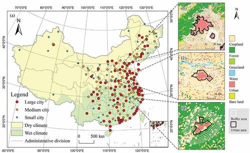
We chose 208 cities in China for an analysis of dominant factors regarding seasonal and diurnal ΔT (Figure 1(a)). It is noteworthy that the analytical procedure excluded cities with urban area of less than 50 km². Moreover, to preserve a comparable number of cities for different sizes and regions, cities in neighboring locations with others were removed from the analysis. Especially, the threshold value of 800 mm yr⁻¹ precipitation was utilized to determine dry and wet climates for the following two reasons. Firstly, the threshold value of 800 mm·yr⁻¹ precipitation is highly consistent with the Qinling Mountains-Huaihe River dividing line, distinguishing the northern and southern parts of China (Zheng 2008; Yang et al. 2017). Secondly, it is close to the 0°C isotherm line in January as well as the line that divides subtropical and temperate monsoon climates. Based on the division line of dry and wet climates, the cities selected were divided into 100 and 108 cities in dry and wet climates, respectively. Following Fang (2014), the cities selected could be further divided into large (population > 1 million), medium (500 thousand < population < 1 million), and small cities (population < 500 thousand) at prefecture-level. The population data was obtained from China Statistical Yearbook 2016 (NBSC (National Bureau of Statistics of China) 2016). The numbers of the large, medium, and small cities are 93, 72, and 43, respectively. It is hard to guarantee exactly equal population distribution among cities, i.e. few small cities can be selected at the prefecture-level.

Figure 1. Overview of the study area: (a) the selected cities, (b) Beijing (large city), (c) Kaifeng (medium city), and (d) Jingdezhen (small city).

2.2 Data sets

Here, we collected MODIS LST products from the National Aeronautics and Space Administration to calculate ΔT. Specifically, we used the MODIS/Aqua version 6 product (i.e. MYD11A2) and MODIS/Terra version 6 product (i.e. MOD11A2) during the period of 2014–2016. Daytime LSTs could be obtained by composing two observations during the daytime (i.e. local time at 1:30 P.M. and 10:30 A.M.). Similarly, nighttime LSTs were composed of two nighttime observations (i.e. local time at 1:30 A.M. and 10:30 P.M.) (Figure S1). The data are 8-day composite LST product and feature fine temporal and spatial coverage (1-km spatial resolution), which is suitable for seasonal and diurnal ΔT exploration at a continental scale (Wan 2014). According to Peng et al. (2012), the LST data features high accuracy and a low root mean square error compared with in-situ observation.

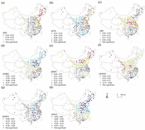
Table 1 shows the driving factors of seasonal ΔT in this study and their distribution can be found in Figure 2. Two-dimensional UMPs, i.e. building coverage (BC), and 3D UMPs, i.e. mean building height (MBH) and mean building volume (MBV), were acquired from (Li et al. 2020a). The data includes building footprint, height, and volume with a spatial resolution of 1-km in 2015. It was retrieved by using the random forest algorithm combining spatial data (e.g. Landsat 8 spectral bands and Sentinel-SAR images) and reference data (e.g. 3D buildings collection from commercial map provider and street view map). Compared with the observation data, the estimated R² values of the building footprint, height, and volume are 0.90, 0.81, and 0.88, respectively (Li et al. 2020a). In addition to UMPs, we also collected socio-economic indices, vegetation, and surface albedo to explore SUHI dynamics. Population density (PD) and nighttime light (NTL) were utilized to represent socio-economic influences. Normalized difference vegetation index (NDVI) and normalized difference water index (NDWI) were chosen to reflect vegetation activities and water content. We selected white sky albedo (WSA) covering shortwave spectrum to represent surface albedo (Peng et al. 2012). Mean annual precipitation was obtained from Global Precipitation Measurement (GPM, Huffman et al. 2019) and used for dry-wet climate division. All MODIS data were averaged over three years (2014–2016) and resampled to a spatial resolution of 1-km to match the LST data.

Figure 2. Spatial distribution of influencing factors used in the study: (a) PD, (b) NTL, (c) BC, (d) MBH, (e) MBV, (f) NDWI, (g) NDVI, and (h) WSA.

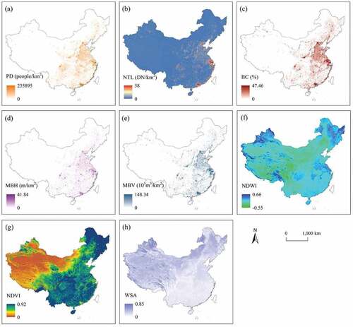
Table 1. Influencing factors of ΔT used in this study.

Category	Variable	Meaning	Source
2D urban morphological parameter	Building coverage (BC)	Percentage of building area in a spatial unit	Li et al. (2020a)
3D urban morphological parameter	Mean building height (MBH)	Average of building height in a spatial unit	Li et al. (2020a)
	Mean building volume (MBV)	Average of building volume	Li et al. (2020a)
Socio-economic index	Population density (PD)	Population density in a spatial unit	Retrieval from Resource and Environmental Science and Data Center (RESDC) (Xu 2017)
	Nighttime light (NTL)	Three year (2014–2016) averaged monthly night light radiance density in a spatial unit	NPP VIIRS monthly product (Elvidge et al. 2017)
Vegetation activity and moisture	NDVI	Three year (2014–2016) averaged normalized difference vegetation index	Retrieval from Resource and Environmental Science and Data Center (RESDC) (Xu 2018)
	NDWI	Three year (2014–2016) averaged normalized difference water index	MCD43A4 MODIS product (Kannan 2019)
Albedo	White sky albedo (WSA)	Three year (2014–2016) averaged albedo of solar diffuse radiation over shortwave broadband (0.3–5.0 μm)	MCD43A4 MODIS product (Wang et al. 2018)

3 Methodology and data

3.1 Overview of methodology

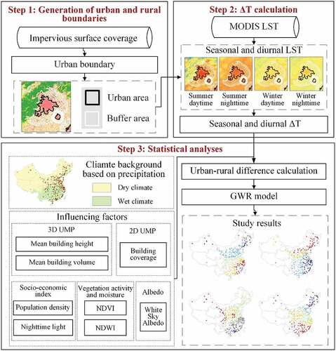
Figure 3 provides the workflow of the study. We tried to explore human-environment interactions in SUHIs and selected the crucial factors associated with urban surface energy balance as of the main drivers, e.g. socio-economic indices, 2D and 3D UMPs, vegetation, and surface albedos. In particular, regional climates and city sizes were chosen as regulating factors to reveal the consequences of human activities and climate settings on seasonal and diurnal SUHIs. As shown in Figure 3, the main steps include the generation of urban and rural boundaries, ΔT calculation, and statistical analyses. The following sections detail the main steps.

Figure 3. The workflow of the analytical procedure.

3.2 Generation of urban and rural boundaries

In this study, the impervious surface coverage of 25% was selected as the threshold to generate urban boundaries (data from Kuang et al. 2020). The reasons are as follows: first, the 25% impervious surface coverage provides a threshold to separate residential areas of medium to high intensity from those of low intensity based on a study in the US (Lu and Weng 2006); Secondly, the 25% impervious surface coverage closely matches the urban area of land use remote sensing monitoring data in 2015 in China from Resource and Environmental Science and Data Center (RESDC) (https://www.resdc.cn/data.aspx?DATAID=184) (Figures 1(b-d)). Rural regions were defined as buffer zones around urban regions (Fu and Weng 2018; Niu et al. 2020). Following Zhou et al. (2015), we tested the impact of rural buffer areas on diurnal ΔT calculation. As shown in Figure S2, stable daytime and nighttime ΔT were observed when rural buffers were designed as 3 and 4 times areas of corresponding urban regions. Therefore, 3 and 4 times areas of urban regions were chosen as rural buffer areas during daytime and nighttime ΔT calculation. Additionally, water bodies, snow, and ice were removed from urban and rural regions to avoid their impacts on ΔT calculation. Moreover, following Imhoff et al. (2010), pixels with elevations exceeding ± 50 m of the median value of elevations in urban regions were also removed to avoid the impacts of elevations. Figures 1(b-d) provide urban and rural boundaries in Beijing, Kaifeng, and Jingdezhen.

3.3 SUHI calculation

We defined diurnal ΔT as the urban-rural differences in LSTs and explored the influences of critical factors regarding urban surface energy balances on summer (from June to August) and winter (from December to February) ΔT (Fu and Weng 2018). The three-year (2014–2016) average LSTs in summer and winter were calculated for both daytime and nighttime. The formula is as follows:

(2) $\mathrm{\Delta }T=T_u-T_r$(2)

where ΔT denotes surface urban heat island intensity and the ΔT in summer daytime, summer nighttime, winter daytime and winter nighttime were denoted as ΔT_sd, ΔT_sn, ΔT_wd and ΔT_wn, respectively; T_u and T_r are the average LSTs in urban and rural areas, respectively.

3.4 Statistical analyses

The urban-rural differences in driving factors, e.g. ΔBC and ΔMBH, were calculated with the same urban and buffer area as ΔT in each city and used as independent variables. In addition, the mean-subtraction method was used before analysis to eliminate the large differences between independent variables (Cai, Huang, and Song 2017):

(3) $x_i^{\ast }=\frac{x_i-\mu }{\sigma }$(3)

where i denotes the i-th city, $x_i^{\ast }$ is the mean-subtracted value of i-th city for each variable, $\mu$ is the average value of each variable, $\sigma$ is the standard deviation of each variable.

We employed GWR models to explore the relationships between driving factors and ΔT. In particular, the SUHI intensities were used as the dependent variable and the independent variables were critical factors involved in surface energy exchanges (Table 1). The GWR model, a local regression model, has the advantage over global regression (e.g. OLS model) in reflecting the spatial distribution characteristics of relationships between variables (Xu, Zhang, and Li 2019; Niu et al. 2021). We further used the GRW model to reveal SUHI variations:

(4) $y_i={\beta }_0\left({\mu }_i,{\vartheta }_i\right)+\sum _{j=1}^k{x}_{ij}{\beta }_j\left({\mu }_i,{\vartheta }_i\right)+{\epsilon }_i,\left(i=1,2,\cdots ,m;j=1,2,\cdots ,k\right)$(4)

where $y_i$, $x_{ij}$, and ε are the dependent variable (i.e. ΔT), the j-th independent variable (i.e. driving factors), and the random error at the city i, respectively. m and k and indicate the number of city and independent variables, respectively. ${\beta }_j\left({\mu }_i,{\vartheta }_i\right)$ is the local regression parameter to be calculated at the location $\left({\mu }_i,{\vartheta }_i\right)$, which represents the longitude and latitude coordinates of the point i. ${\beta }_0\left({\mu }_i,{\vartheta }_i\right)$ is the geographically varying intercept.

The weights of independent variables in GWR models were estimated by the function of the distance from point i. Generally, nearby locations will be assigned higher weights than distant ones (Dziauddin 2019). Thus, the weights of independent variables change in a specific space, namely, the spatial kernel. The extent of the spatial kernel is also called bandwidth. There are two methods to construct a spatial kernel: fixed distance and adaptive method. The fixed distance method uses a fixed bandwidth to solve each local regression. In contrast, the adaptive method selects a specified number of neighbors to construct a spatial kernel. The denser the spatial distribution of regression location (i.e. the selected cities) is, the fewer the neighbor is. Here, we used the fixed kernel type to build GWR models due to the even and dense distribution of selected cities. To diagnose the performances of GWR models, we determined the coefficient of determination (R²), Akaike Information Criterion (AICc) and standardized residual of models. In addition, the spatial autocorrelation of residuals was tested by Moran’s Index (MI).

4 Results

4.1 Seasonal and diurnal changes in SUHIs

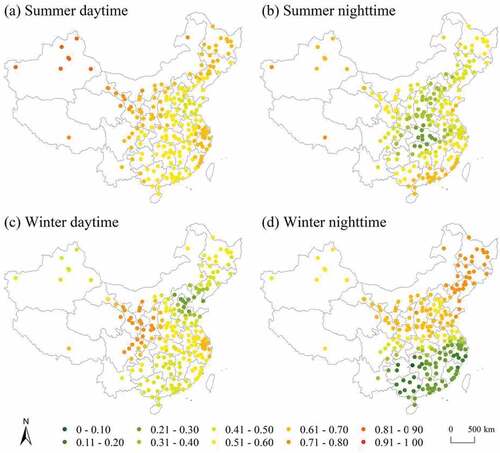
Figure 4(a) shows that positive ΔT was observed in most cities during summer daytime (> 95%). About 30% of the cities selected yielded large ΔT_sd (higher than 3°C). In addition, some cities associated with negative ΔT_sd were observed in China’s northwestern part, such as Jiayuguan (−2.29°C) and Hami (−0.57°C). Figure 4(b) shows that most cities had positive ΔT during summer nighttime (> 99%). Medium ΔT_sn (1 < ΔT_sn < 2°C) was observed in 67% of cities. Only 17 cities, mainly in dry climates, yielded large ΔT_sn. It is noteworthy that, in summer, the daytime ΔT was higher than that at night (Figures 4(a,b), which may be due to the underlying surfaces absorbing solar radiations and producing more anthropogenic heat (e.g. air conditioning cooling) during the daytime.

Figure 4. Spatial distribution of seasonal and diurnal ΔT over 208 cities in China, 2014–2016: (a) ΔT_sd, (b) ΔT_sn, (c) ΔT_wd, (d) ΔT_wn, and mean ΔT under varying city sizes in dry (e) and wet (f) climates.

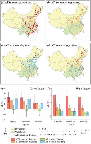
In winter, about 39% of cities yielded negative daytime ΔT. Those cities are mainly located in dry climates, such as Lhasa (−1.90°C), Tongliao (−1.75°C), and Panjin (−0.57°C). However, in wet climates, most cities produced positive ΔT_wd (Figure 4(c)). At night, large ΔT_wn was found in dry climates. Additionally, in wet climates, a similar ΔT distribution at night was found compared with that in daytime (Figure 4(d)). Interestingly, nighttime ΔT was observed higher than daytime ΔT in winter (especially in dry climates), and this differs in summer diurnal cycles (Figures 4(c,d)). In winter nighttime, cities in dry climates would produce more anthropogenic heat (i.e. heating in winter) than those in wet climates. Figures 4(e,f) show the average ΔT under varying city sizes in dry and wet climates. First, the city size can significantly impact the average ΔT in seasonal and diurnal cycles. Usually, a larger city size produces a higher ΔT. Notably, average summer daytime ΔT in wet climates was higher than that in dry climates. The possible reason is that, in dry climates, rural areas often have sparse vegetation, leading to limited heat mitigation of vegetation. In contrast, high-rise buildings in urban areas can enhance the efficiency of land-air convection, e.g. increasing shading of ground surfaces and accelerating air convection. All of these lead to low summer daytime SUHIs in dry climates. Meanwhile, average nighttime ΔT in wet climates was lower than that in dry climates, which could be explained by the warming effect of dense vegetation (compared with soils in dry climates) on rural LSTs in wet climates. It indicates that the influence of driving factors on ΔT may vary by different climates and by varying seasonal and diurnal cycles.

4.2 Diagnostics of GWR models

We inspected the correlations between the chosen variables using the variance inflation factors (VIFs, revealed by the OLS model) and correlation matrix to determine the multicollinearity level in our models. The VIFs are displayed in Table S1, which shows all VIFs of variables were below 10, indicating that no redundant variables were observed in the regression. Table S2 shows the correlation matrix concerning variables involved in analyses. As shown, most of the correlation values were below 0.5, indicating the chosen variables did not suffer multicollinearity.

Table 2 shows the diagnostics of GWR models. As shown, seasonal and diurnal variations in adjusted determination coefficient (R²) were observed, indicating that influencing factors used in the study had different total variance explained in seasonal and diurnal cycles. Overall, low Akaike information criterion (AICc) and root mean squared error (RMSE) values in GWR models were observed. It suggests the excellent performance of the models selected in revealing ΔT spatial variations, especially in summer daytime (AICc: 324.23; RMSE: 0.43) and winter nighttime (AICc: 358.46; RMSE: 0.43). In addition, the Moran’s I (MI) of standardized residuals was close to 0 in GWR models (p-value < 0.05), suggesting that the residuals feature no evident spatial autocorrelation.

Table 2. Diagnostics of GWR models.

Variable	Summer		Winter
	Daytime	Nighttime	Daytime	Nighttime
R^2	0.82	0.73	0.74	0.81
Adjusted R^2	0.77	0.63	0.67	0.74
AICc	324.23	434.70	391.26	358.46
RMSE	0.43	0.52	0.51	0.43
MI of standardized residuals	0.0070	0.0206	0.0397	0.0052
MI Probability (p-value)	0.0034	0.0027	0.0001	0.0098

Table 3 shows the mean absolute values of the T-statistic tests regarding driving factors using GWR models. As shown, the mean absolute values of the T-statistic test concerning ΔBC, ΔMBH, ΔMBV, and ΔWSA were higher than the threshold value of 1.96 in different periods, indicating these factors were statistically significant at the level of 0.05 for seasonal and diurnal ΔT. Notably, ΔNDVI had the highest mean absolute value of the T-statistic test in summer daytime (4.52), indicating ΔNDVI can significantly influence the spatial variations in ΔT_sd. In addition, ΔPD was statistically significant for ΔT_sd and ΔT_wn (i.e. the mean absolute value > 1.96), ΔNTL was statistically significant for ΔT_wn and ΔNDWI was statistically significant for ΔT_sd and ΔT_sn.

Table 3. Results of the T-statistic test concerning driving factors for explaining seasonal and diurnal ΔT using GWR models.

Driving factors	Summer		Winter
	Daytime	Nighttime	Daytime	Nighttime
ΔPD	2.10	1.66	1.55	2.03
ΔNTL	1.45	1.31	1.58	2.29
ΔBC	2.37	2.03	2.90	2.28
ΔMBH	2.11	2.76	3.14	2.69
ΔMBV	2.43	2.97	3.30	3.29
ΔNDVI	4.52	3.02	2.12	1.95
ΔNDWI	1.63	1.10	2.74	2.50
ΔWSA	4.41	3.06	4.04	3.75

Figure 5 shows the local R² values of each city in GWR models under varying seasonal and diurnal settings. As shown, the performance of the GWR model in summer daytime (the local R² values changed from 0.4 to 0.9) was better than that in other periods, indicating the driving factors used can better explain ΔT_sd spatial variations (Figure 5(a)). Low R² values were observed in China’s central parts in summer nighttime, suggesting more influencing factors should be considered for ΔT_sn explanations in these regions (Figure 5(b)). Similarly, in winter daytime, Beijing, Tianjin, and Tangshan regions were associated with low local R² values (Figure 5(c)). Notably, significant differences in local R² values of ΔT_wn were observed between dry and wet climates, indicating that, in winter nighttime, climatic division can influence the performance of crucial factors regarding urban surface energy balance to control SUHI intensities (Figure 5(d)).

Figure 5. Spatial distribution of the local R² values revealed by GWR models: (a) summer daytime, (b) summer nighttime, (c) winter daytime, and (d) winter nighttime.

4.3 Relationships between seasonal and diurnal ΔT and driving factors

Figure 6 shows the spatial distribution of the regression coefficient (β) values concerning driving factors in summer daytime. As shown, ΔPD was positively correlated with ΔT_sd, and a high β value in dry climates (β value = 0.27 ± 0.08, Table 4) was observed. However, it was found that the ΔPD influence was non-significant (p-value > 0.05) in most cities in wet climatic settings (Figure 6(a)). Additionally, slightly positive correlations between ΔNTL and ΔT_sd were observed in 26.92% of municipalities, mainly located in eastern China with rapid economic developments and dense human activities (Figure 6(b)). Cities in this region generate more anthropogenic heats, leading to the rising ΔT_sd. These findings suggest high human activity intensities can increase summer daytime ΔT, but the increase varied by regional climates and spatial variations.

Figure 6. Regression coefficient (β) values of driving factors in summer daytime by GWR models: (a) ΔPD, (b) ΔNTL, (c) ΔBC, (d) ΔMBH, (e) ΔMBV, (f) ΔNDWI, (g) ΔNDVI, and (h) ΔWSA.

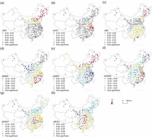
Table 4. Mean and standard deviation of regression coefficient values (β) in seasonal and diurnal cycles and proportion of significant results of each driving factor under varying climates based on GWR models.

	ΔPD	ΔNTL	ΔBC	ΔMBH	ΔMBV	ΔNDWI	ΔNDVI	ΔWSA
Summer daytime ΔT
Dry climate	0.27 (0.08)	0.06 (0.11)	0.29 (0.06)	−0.37 (0.12)	0.27 (0.16)	−0.17 (0.08)	−0.60 (0.08)	0.19 (0.13)
Significance proportion (%)	85.00	28.00	43.00	63.00	90.00	80.00	100.00	96.00
Wet climate	0.09 (0.02)	0.12 (0.07)	0.28 (0.05)	−0.18 (0.11)	0.13 (0.12)	−0.10 (0.07)	−0.25 (0.05)	0.43 (0.12)
Significance proportion (%)	10.18	34.26	95.37	96.30	87.96	69.44	84.26	100.00
Total city	0.18 (0.10)	0.09 (0.08)	0.28 (0.04)	−0.27 (0.13)	0.20 (0.14)	−0.13 (0.06)	−0.42 (0.10)	0.32 (0.15)
Significance proportion (%)	41.82	26.92	65.87	77.40	88.94	70.19	91.83	98.08
Summer nighttime ΔT
Dry climate	0.19 (0.10)	0.14 (0.06)	0.27 (0.19)	−0.30 (0.08)	0.38 (0.06)	0.10 (0.16)	−0.32 (0.15)	−0.33 (0.10)
Significance proportion (%)	57.00	6.00	43.00	82.00	84.00	0.00	100.00	91.00
Wet climate	0.13 (0.06)	0.18 (0.03)	0.21 (0.07)	−0.15 (0.11)	0.26 (0.10)	−0.04 (0.03)	−0.22 (0.10)	−0.15 (0.18)
Significance proportion (%)	10.19	56.48	93.51	93.51	92.59	87.04	91.67	100.00
Total city	0.16 (0.13)	0.16 (0.05)	0.24 (0.14)	−0.22 (0.12)	0.32 (0.12)	0.03 (0.11)	−0.27 (0.20)	−0.24 (0.17)
Significance proportion (%)	28.37	27.36	69.23	87.98	88.46	39.90	95.67	95.67
Winter daytime ΔT
Dry climate	0.27 (0.06)	0.13 (0.08)	0.17 (0.06)	−0.45 (0.11)	0.39 (0.08)	−0.19 (0.14)	−0.17 (0.10)	−0.17 (0.18)
Significance proportion (%)	81.00	42.00	59.00	100.00	90.00	99.00	37.00	91.00
Wet climate	0.12 (0.03)	0.26 (0.05)	0.13 (0.04)	−0.14 (0.09)	0.24 (0.06)	−0.09 ± 0.05	−0.11 ± 0.10	−0.01 ± 0.21
Significance proportion (%)	14.81	26.85	87.96	97.22	96.30	56.48	58.33	100.00
Total city	0.20 (0.11)	0.20 (0.07)	0.15 (0.05)	−0.30 (0.15)	0.32 (0.12)	−0.14 (0.12)	−0.14 (0.12)	−0.09 (0.20)
Significance proportion (%)	42.31	32.21	74.04	97.60	93.27	73.56	48.08	95.67
Winter nighttime ΔT
Dry climate	0.16 (0.10)	0.22 (0.06)	0.16 (0.16)	−0.44 (0.07)	0.40 (0.12)	0.22 (0.10)	−0.23 (0.07)	−0.18 (0.06)
Significance proportion (%)	60.00	65.00	62.00	100.00	98.00	100.00	41.00	100.00
Wet climate	0.08 (0.06)	0.15 (0.07)	0.08 (0.07)	−0.12 (0.03)	0.20 (0.08)	0.03 (0.11)	−0.11 (0.10)	−0.09 (0.11)
Significance proportion (%)	28.70	62.04	49.07	46.30	42.30	46.30	30.56	80.56
Total city	0.12 (0.09)	0.18 (0.06)	0.12 (0.11)	−0.28 (0.10)	0.30 (0.12)	0.13 (0.12)	−0.17 (0.12)	−0.14 (0.13)
Significance proportion (%)	40.38	62.50	50.96	67.79	64.90	70.19	30.29	86.54

Favorably positive links between ΔBC and ΔT_sd were observed in China’s northeastern parts (the highest β value = 0.40, Figure 6(c)), suggesting the warming effects of building coverages in summer daytime. As shown in Figure 6(d), ΔMBH was highly negatively correlated with ΔT_sd, and more substantial influences of ΔMBH in dry climates (β = −0.37 ± 0.12, Table 4) was observed than those in wet climates (β = −0.18 ± 0.11, Table 4). The potential reason is that buildings cast shadows and accelerate air convection can reduce surface temperatures in urban areas. It might be more pronounced in dry climates because of the sparse vegetation and low solar altitude angle. As shown in Figure 6(e), positive links between ΔMBH and ΔT_sd were observed and the links were stronger in dry climates (β = 0.27 ± 0.16, Table 4) than those in wet climates (β = 0.13 ± 0.12, Table 4).

ΔNDWI was slightly negatively correlated with ΔT_sd (β = −0.13 ± 0.06, Figure 6(f) and Table 4), suggesting vegetation moisture contents can mitigate surface warming to some extents. Additionally, a strong negative correlation between ΔNDVI and ΔT_sd was observed, especially in dry environments (minimum β value = −0.99) (Figure 6(g)), indicating vegetation coverage is a crucial cooling factor in summer daytime. It was found ΔWSA was positively correlated with ΔT_sd (Figure 6(h)). Generally, higher urban-rural differences in albedo should reduce the energy absorbed by urban areas, leading to the reduction of SUHIs. However, low vegetation covers can increase albedo to some extent since vegetation components are “darker” than most built-up structures. This may lead to a positive correlation between ΔWSA and ΔT_sd.

Figure 7 provides the β spatial distribution of driving factors in summer nighttime. A similar influence of ΔPD on nighttime ΔT was found compared with daytime (Figure 7(a)). Additionally, ΔNTL was positively correlated with ΔT_sn in China’s southeastern parts, which was consistent with that in daytime (Figure 7(b)). These findings suggest human activities yielded a similar impact on ΔT in summer diurnal cycles.

Figure 7. Regression coefficient values (β) of driving factors by GWR models in summer nighttime: (a) ΔPD, (b) ΔNTL, (c) ΔBC, (d) ΔMBH, (e) ΔMBV, (f) ΔNDWI, (g) ΔNDVI, and (h) ΔWSA.

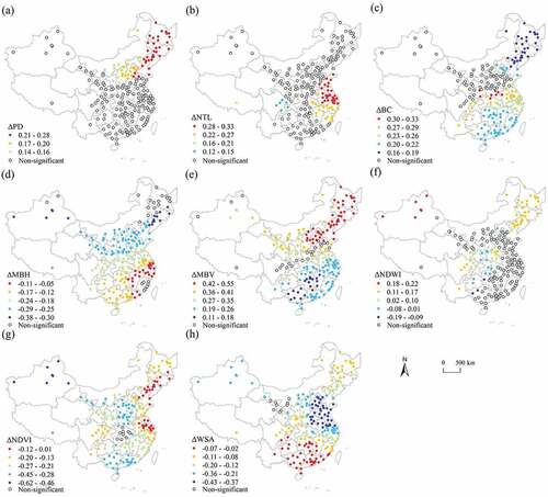
As shown in Figure 7(c), the positive link between ΔBC and ΔT in nighttime (β = 0.21 ± 0.07, Table 4) was weaker than that in daytime (β = 0.28 ± 0.05, Table 4), indicating 2D UMP exerts more warming impact on daytime ΔT than that on nighttime ΔT. As to 3D UMPs, it was found that ΔMBH was negatively correlated with ΔT_sn. In addition, under the dry climatic setting, the mitigation effects of building height on daytime ΔT (β = −0.37 ± 0.07, Table 4) were higher than that on nighttime ΔT (β = −0.30 ± 0.08, Table 4) (Figure 7(d)). As shown in Figure 7(e), a positive correlation between ΔMBV and ΔT_sn was found, and building volume yielded more warming effects on nighttime surfaces (β = 0.32 ± 0.12, Table 4) than daytime surfaces (β = 0.20 ± 0.14, Table 4).

It is noteworthy that slight positive correlations between ΔNDWI and ΔT_sn were observed in dry climates (β = 0.10 ± 0.16, Table 4), which differs in summer daytime (β = −0.17 ± 0.08, Table 4) (Figure 7(f)). It suggests that distinguishable roles of ΔNDWI are played in surface energy balance during summer diurnal cycles. Generally, ΔNDVI significantly mitigated ΔT during summer diurnal cycles (Figure 7(g)); however, the cooling effects of ΔNDVI on underlying daytime surfaces (β = −0.42 ± 0.10, Table 4) were observed higher than those on nighttime surfaces (β = −0.27 ± 0.20, Table 4). Notably, ΔWSA yielded strongly negative influences on ΔT_sn in the cities selected (β = −0.24 ± 0.17), suggesting a crucial cooling effect of ΔWSA on ΔT_sn (Figure 7(h) and Table 4). The possible reason is that a lower albedo leads to higher ground heat storage, and this heat is released at night, increasing the nighttime SUHI.

Figure 8 shows the β spatial distribution of different influencing factors in winter daytime. As shown in Figure 8(a), ΔPD was highly correlated with ΔT_wd (β = 0.20 ± 0.11, Table 4). Additionally, the warming effects of ΔNTL in winter daytime (β = 0.20 ± 0.07, Table 4) were higher than those in summer daytime (β = 0.09 ± 0.08, Table 4) (Figure 8(b)). These findings suggest that, as typical heating factors, human activities in winter can exert more decisive influences on ΔT than those in summer. As to 2D UMP, the positive correlation between ΔBC and ΔT_wd in dry climatic settings (the highest β value = 0.25) was observed more substantial than that in wet environments (β = 0.13 ± 0.04, Figure 8(c) and Table 4). In addition, the correlation in winter daytime (β = 0.15 ± 0.05, Table 4) was found lower than that in summer daytime (β = 0.28 ± 0.04, Table 4), suggesting that building coverage yields more warming effects on Earth’s skins in summer than those in winter. As to 3D UMPs, negative correlations between ΔMBH and ΔT_wd in high-latitude regions (i.e. dry climates, β = −0.45 ± 0.11) were observed higher than those in low-latitude regions (i.e. wet climates, β = −0.14 ± 0.09) (Figure 8(d)). The possible reason is that cities in high-latitude regions can cast large building shadows and thus reduce surface temperatures in urban areas. As shown in Figure 8(e), ΔMBV was highly positively correlated with ΔT_wd, and the correlation in dry climates was found higher than that in wet climates (Table 4).

Figure 8. Regression coefficient values (β) of driving factors by GWR models in winter daytime: (a) ΔPD, (b) ΔNTL, (c) ΔBC, (d) ΔMBH, (e) ΔMBV, (f) ΔNDWI, (g) ΔNDVI, and (h) ΔWSA.

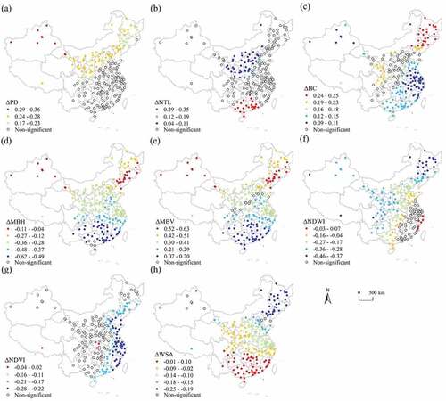
It was found that ΔNDWI was negatively correlated with ΔT_wd (β = −0.14 ± 0.12, Figure 8(f) and Table 4). Additionally, it was highly negatively correlated with ΔT_wd in the northeastern parts of China (the minimum β value = −0.46), which could partly be explained by the vegetation created by special water and energy conditions in high latitudes (Sun et al. 2013). The negative correlation between ΔNDVI and ΔT_wd in winter daytime (β = −0.14 ± 0.12) was lower than in summer daytime (β = −0.42 ± 0.10, Figure 8(g) and Table 4). Notably, ΔWSA showed a weak negative correlation with ΔT_wd in the cities selected (β = −0.09 ± 0.20), which differs from that in summer daytime (Figure 8(h) and Table 4).

Figure 9 provides the β spatial distribution of driving factors revealed by GWR models in winter nighttime. As shown in Figure 9(a), a weakly positive correlation between ΔPD and ΔT_wn was observed (β = 0.16 ± 0.10, Table 4), and the correlation in winter nighttime was lower than that in other periods, e.g. summer nighttime. It was found that highly positive correlations between ΔNTL and ΔT_wn in coastal cities in China’s northern parts (the highest β value = 0.36, Figure 9(b)), which differs from those in winter daytime.

Figure 9. Regression coefficient values (β) of driving factors by GWR models in winter nighttime: (a) ΔPD, (b) ΔNTL, (c) ΔBC, (d) ΔMBH, (e) ΔMBV, (f) ΔNDWI, (g) ΔNDVI, and (h) ΔWSA.

ΔBC showed slight positive correlations with ΔT_wn (β = 0.12 ± 0.11, Table 4 and Figure 9(c)), lower than those in other periods. It suggests that the warming effects of building coverage are not evident compared with those in different periods, e.g. winter daytime. As to 3D UMPs, the links between 3D UMPs and ΔT_wn were similar to those in daytime, i.e. 3D UMPs in dry climates yielded higher impacts on ΔT than those in wet climates (Figures 9(d,e)). It indicates that the influence of 3D UMPs on surface energy balances exist in diurnal inertia to some extent. Notably, positive correlations between ΔNDWI and ΔT_wn were observed in dry climates (β = 0.22 ± 0.10, Figures 9(f) and Table 4), suggesting a warming effect of vegetation moisture on ΔT_wn. Still, ΔNDVI and ΔWSA were negatively correlated with ΔT_wn (Figures 9(g,h)), presenting their cooling effects in winter nighttime.

5 Discussion

5.1 Influence of UMPs on seasonal and diurnal SUHIs: 2D vs. 3D

In this study, it was found that 3D UMPs (i.e. ΔMBH and ΔMBV) yielded more decisive influences on ΔT than 2D UMP (i.e. ΔBC); this is particularly true in summer day-night cycles and under a dry climatic setting. Our finding is in line with an investigation of the influence of urban structures (including 2D and 3D) on LSTs using remotely sensed observations by Ezimand, Azadbakht, and Aghighi (2021). Thus, it is essential to improve 3D UMPs to perform SUHI mitigations (He et al. 2021). Additionally, ΔBC and ΔMBV exerted significantly warming effects on Earth’s skins. The possible reason is that buildings featured as impervious surfaces can absorb shortwave solar energy during the daytime and release it into atmospheres during the nighttime, leading to warming effects on underlying surfaces during diurnal cycles (Manoli et al. 2019; Hong et al. 2020; Morabito et al. 2021; Taurines et al. 2021). Meanwhile, building energy consumption increases anthropogenic heat emissions, resulting in SUHI rising (Santamouris 2014; Yu et al. 2021; Yang and Li 2013; Ye et al. 2021).

Seasonal variations in the impacts of 2D and 3D UMPs on ΔT were observed. The warming effects of ΔBC in summer were more substantial than those in winter. The possible reason is that buildings absorb higher solar radiation and create fewer building shadows in summer than in winter (Khamchiangta and Dhakal, 2019). However, the cooling effect of ΔMBH in winter was higher than in summer, partly because of the lower solar elevation angle in winter (Huang and Yang, 2019; He et al. 2021; Li et al. 2021). Beyond this, vegetation evapotranspiration becomes weak in winter; thus, the cooling effects of the land-air convection caused by building roughness determine the SUHI mitigation in winter (Berger et al. 2017; Niu et al. 2021).

For the diurnal cycle of SUHIs, we found that the warming effect of 2D UMP on ΔT exhibits consistency during day and night observations, which is consistent with Zhou et al. (2014). However, significantly various performances of ΔMBH and ΔMBV on ΔT were found during diurnal cycles. ΔMBH can mitigate ΔT by casting shadows, which has been proved by Li et al. (2021). Therefore, the giant building shadows on surfaces can explain the more substantial cooling effect of the ΔMBH in daytime. In addition, the notable warming effect of ΔMBV on nighttime ΔT indicates that buildings would release more anthropogenic heat at night, which could generate heat upward to the atmosphere and then contribute to surface warming (Hu et al. 2019; Hong et al. 2020; Yao et al. 2021b).

5.2 The modification of climatic factors

Using GWR models, we revealed the spatial variations in the influences of dominant factors regarding ΔT under dry-wet climatic settings. It was found that ΔBC yielded a low warming effect on winter ΔT in wet environments (Figures 9(c)). The possible reason is that, in winter, building areas feature lower heat storage abilities than their rural settings with wet soil environments (Zhao et al. 2014; He et al. 2021). Additionally, the cooling effects of ΔMBH in the dry climate were higher than those in the wet climate (Figures 6-Figures 9(d)). Previous studies have demonstrated that tall buildings could increase the land-air convection efficiency to help SUHI mitigations (Berger et al. 2017; Huang and Wang 2019; Yu et al. 2020; Budhiraja, Gawuc, and Agrawal 2019; Sun et al. 2020). In particular, in the dry climate, the cooling effects of low and sparse vegetation are limited. Thus, building roughness plays a critical role in surface cooling by increasing land-air convection efficiency. We also found that ΔMBV yielded a higher warming effect on winter ΔT in dry climates than that in wet climates (Figures 8(e) and 9(e)). It is because high latitude cities in China during heating periods could produce more anthropogenic heat emissions and thus increase winter SUHI.

The cooling effect of ΔNDVI in dry climates (β = −0.60 ± 0.08) was higher than that in wet climates (β = −0.25 ± 0.05) in summer daytime (Figure 6(h) and Table 4). This finding is in line with (Manoli et al. 2019). The possible reason is that the cooling effect of vegetation evapotranspiration is more considerable for regions with low average precipitations and soil water contents (Buyantuyev and Wu 2012; Imhoff et al. 2010; Wang et al. 2015). Additionally, ΔWSA in summer daytime yielded higher warming effects on ΔT in wet climates than in dry climates (Figures 6h). The reasons can be attributed to the fact that a high WSA is often associated with higher building coverage, contributing to rising surface temperature (Bonafoni, Baldinelli, and Verducci 2017; Zhou et al. 2019; Sekertekin et al., 2021). Cities in wet climates are often surrounded by evergreen forests and croplands, which enlarge ΔWSA and thus significantly increase ΔT. Moreover, ΔWSA yielded cooling effects on winter ΔT in dry climates. It can be explained by the high brightness of bare soils featuring high albedo in the dry climate, which could help surface cooling (Haashemi et al. 2016).

5.3 Influence of city size on SUHIs

Generally speaking, in dry climates, ΔT in large and medium cities was observed higher than in small cities (Figures 4(e,f)). Large and medium cities produce more anthropogenic heat than small cities; additionally, cities in dry climates feature high thermal inertia, increasing surface temperatures by storing latent heat (Clinton and Gong 2013). In wet climates, small cities are usually surrounded by tall and dense vegetation, leading to a high evaporation rate and LST mitigations in rural areas (Ward et al. 2016). Meanwhile, building heights in small cities are often lower than those in large and medium cities, resulting in low land-air convection efficiencies in urban areas (Berger et al. 2017; Manoli et al. 2019).

In addition, the regulation of city sizes on ΔT was tested in this study. Table 5 provides the average and standard deviation of β values in different city sizes. As shown in Table 5, the influences of 2D UMP (e.g. ΔBC), 3D UMPs (e.g. ΔMBH and ΔMBV), and human activities (e.g. ΔPD) on seasonal and diurnal ΔT in large cities were more substantial than those in medium and small cities. Additionally, it was found that ΔNDVI can help SUHI mitigation more in small cities. This finding is important since it suggests that the regulation of UMPs and population in large cities yields a better effect than in small cities (Yao et al. 2021a). In contrast, urban greening could help surface cooling in small cities more than in large cities.

Table 5. The average and standard deviation of β value and proportion of significant results across different city sizes.

City size	ΔPD	ΔNTL	ΔBC	ΔMBH	ΔMBV	ΔNDWI	ΔNDVI	ΔWSA
Summer daytime
Large city	0.20 (0.09)	0.09 (0.03)	0.28 (0.02)	−0.29 (0.21)	0.21 (0.09)	−0.15 (0.04)	−0.38 (0.08)	0.27 (0.09)
Significance proportion (%)	35.48	34.40	62.36	82.79	88.17	62.36	92.47	98.92
Medium city	0.17 (0.10)	0.10 (0.03)	0.28 (0.03)	−0.24 (0.20)	0.19 (0.11)	−0.13 (0.03)	−0.38 (0.09)	0.27 (0.10)
Significance proportion (%)	40.28	26.39	72.22	77.78	88.89	77.78	90.27	97.22
Small city	0.14 (0.08)	0.06 (0.04)	0.27 (0.01)	−0.22 (0.19)	0.18 (0.11)	−0.08 (0.06)	−0.44 (0.12)	0.32 (0.05)
Significance proportion (%)	58.14	11.63	62.79	65.11	90.70	74.42	93.02	97.67
Summer nighttime
Large city	0.19 (0.12)	0.19 (0.11)	0.24 (0.13)	−0.26 (0.10)	0.33 (0.07)	0.05 (0.13)	−0.29 (0.08)	−0.28 (0.10)
Significance proportion (%)	24.73	37.63	77.42	90.32	86.02	39.78	94.62	97.85
Medium city	0.15 (0.06)	0.17 (0.08)	0.21 (0.17)	−0.20 (0.08)	0.30 (0.11)	0.02 (0.04)	−0.26 (0.10)	−0.25 (0.12)
Significance proportion (%)	31.94	22.22	69.44	91.67	90.28	45.83	94.44	95.83
Small city	0.12 (0.07)	0.14 (0.09)	0.20 (0.09)	−0.19 (0.11)	0.29 (0.10)	0.00 (0.09)	−0.23 (0.10)	−0.23 (0.09)
Significance proportion (%)	30.23	16.28	51.16	76.74	90.70	30.23	100.00	90.70
Winter daytime
Large city	0.23 (0.16)	0.23 (0.12)	0.17 (0.04)	−0.33 (0.15)	0.35 (0.10)	−0.16 (0.14)	−0.14 (0.08)	−0.24 (0.07)
Significance proportion (%)	27.96	31.18	76.34	95.70	95.70	67.74	63.44	95.70
Medium city	0.19 (0.13)	0.21 (0.08)	0.15 (0.06)	−0.30 (0.12)	0.33 (0.09)	−0.15 (0.05)	−0.13 (0.12)	−0.23 (0.12)
Significance proportion (%)	47.22	31.94	69.44	98.61	90.28	72.22	38.89	98.61
Small city	0.17 (0.11)	0.18 (0.09)	0.12 (0.05)	−0.26 (0.05)	0.28 (0.07)	−0.11 (0.11)	−0.16 (0.10)	−0.26 (0.05)
Significance proportion (%)	65.12	34.88	76.74	100.00	93.02	88.37	30.23	90.70
Winter nighttime
Large city	0.14 (0.07)	0.20 (0.09)	0.13 (0.11)	−0.29 (0.12)	0.34 (0.15)	0.15 (0.09)	−0.18 (0.13)	−0.15 (0.08)
Significance proportion (%)	45.16	68.81	54.84	64.52	54.84	69.89	21.51	81.72
Medium city	0.11 (0.09)	0.16 (0.11)	0.11 (0.13)	−0.28 (0.05)	0.31 (0.10)	0.14 (0.13)	−0.18 (0.11)	−0.14 (0.12)
Significance proportion (%)	30.56	54.17	48.61	69.44	68.06	69.44	33.33	87.50
Small city	0.09 (0.10)	0.14 (0.07)	0.10 (0.08)	−0.22 (0.04)	0.27 (0.09)	0.11 (0.07)	−0.16 (0.03)	−0.12 (0.10)
Significance proportion (%)	46.51	62.79	46.51	72.09	81.40	72.09	44.19	95.35

5.4 Limitations and future research directions

We noted several limitations in this study. Firstly, we investigated the influences of 2D and 3D UMPs on seasonal and diurnal ΔT at a 1-km spatial scale to match the resolution of MODIS LST and other remotely sensed products that were used as driving parameters. Our study has considerable limitations in revealing 2D and 3D urban forms at the city-block scale, leaving uncertain driving analysis results (Bhatta, Saraswati, and Bandyopadhyay 2010). For instance, ΔMBH and its impacts on ΔT may underestimate in large cities due to the coarse resolution and averaging process in urban areas. Therefore, studies exploring the influences of 2D and 3D UMPs on ΔT with more satisfactory spatial resolution over a large scale are required.

Secondly, several advantages of GWR models are worthy of declaring and can be summarized as follows. Firstly, GWR models could better reveal the spatial heterogeneity of driving factors than global regression models. Secondly, GWR models can reflect the distinctive roles of driving factors under varying climate settings and across different sizes (Tables 4 and 5), e.g. we found that ΔMBH yielded a higher cooling effect on ΔT_sd in dry climates than in wet climates. However, the R² values of GWR models were lower than 0.5 in several cities (Figure 5), implying that current variables cannot fully explain ΔT in some regions. Factors, including landscape pattern, wind speed, solar radiation, and analyses at different spatial scales (e.g. city blocks), should be investigated in future studies (He et al. 2021; Li et al. 2021). Notably, in related research, the analytic results regarding the influence of critical factors on SUHIs should be carefully verified. Otherwise, we may reach misleading conclusions. For example, our results showed a positive correlation between ΔWSA and summer daytime SUHI, which makes no sense since higher urban-rural differences in albedo should reduce daytime SUHI by decreasing underlying surfaces’ energy absorbed (Chakraborty, Sarangi, and Lee 2021). The possible reason for this statistical bias is probably the relation between albedo and vegetation.

Thirdly, the coarse division of urban-rural boundaries may lead to some uncertainty due to the heterogeneous surfaces in urban and rural areas (Stewart and Oke 2012). Combining the surface structure, cover, and human activities with local climate zones (LCZs) can provide a standard framework for reporting and comparing air/surface temperature observations (Zhao et al. 2019, 2020).

6 Conclusions

In this study, the spatiotemporal patterns of seasonal and diurnal ΔT over 208 cities in China were investigated under varying climates and city sizes. We explored how key factors controlling the urban surface energy balance, i.e. socio-economic indices, 2D and 3D UMPs, vegetation, and surface albedos, impact seasonal and diurnal ΔT from 2014 to 2016. Regional climates and city sizes were further employed to reveal the consequences of human activities and climate settings on seasonal and diurnal cycles of ΔT. The main conclusions can be drawn as follows.

• The 3D UMPs (i.e. ΔMBH and ΔMBV) yielded more decisive influences on ΔT than the 2D UMP (i.e. ΔBC); this is particularly true in the dry climate. The cooling effects of ΔMBH on ΔT in dry climates were higher than in wet climates. The warming effects of ΔMBV on ΔT_wn in dry climates (β = 0.40 ± 0.12) were significantly higher than those in wet climates (β = 0.20 ± 0.08).

• The cooling effect of ΔNDVI on ΔT_sn in dry climates (β = −0.32 ± 0.15) was higher than that in wet climates (β = −0.22 ± 0.10). ΔWSA was positively (negatively) correlated with ΔT_sd (ΔT_sn). The socio-economic indices, i.e. ΔPD and ΔNTL, had warming effects on seasonal and diurnal ΔT. Population density was an important heating factor in the northern part of China. In contrast, night light intensity mainly increased ΔT in the southeastern part of China.

• Varying control patterns of dominant factors were observed in different climates and city sizes. The regulation of UMPs to control urban thermal environments in large cities yielded a better effect than in small cities. In addition, urban greening could help surface cooling in small cities more than in large cities (in dry climates more than in wet climates).

The study contributed to UHI studies in the following aspects. Firstly, the study provides a clear picture of the influence of various driving factors, especially 3D UMPs, on seasonal and diurnal ΔT at a large scale. Secondly, how human activities and climatic settings have interacted to modify the influence of these factors on the urban surface energy balance was determined. The finding suggests that urban thermal regulations should consider climate backgrounds and population sizes. Finally, we employed GWR models to reveal the varying influences of driving factors under different climatic settings and city sizes.

Highlights (for review)

• Driving factors of seasonal and diurnal surface urban heat islands were investigated under varying climates by geographically weighted regression models

• Urban-rural difference in building height and volume yielded more decisive influence on surface urban heat islands than that in building coverage

• The warming effect of building coverage in summer stronger than that in winter

• Building height can be used to mitigate urban thermal environments, especially in dry climates

Nomenclature

Table

Nomenclature	Definition
Δ	Urban-rural difference
β	Regression coefficient value
2D	Two-dimensional
3D	Three-dimensional
AIC	Akaike Information Criterion
ASTER	Advanced spaceborne thermal emission and reflection radiometer
CV	Cross validation
GPM	Global precipitation measurement
GWR	Geographically Weighted Regression
BC	Building coverage
LST	Land surface temperature
MBH	Mean building height
MBV	Mean building volume
MI	Moran’s index
MODIS	Moderate-resolution imaging spectroradiometer
NASA	National Aeronautics and Space Administration
NBSC	National Bureau of Statistics of China
NDVI	Normalized difference vegetation index
NDWI	Normalized difference water index
NTL	Nighttime light
OLS	Ordinary Least Square
PD	Population density
R^2	The coefficient of determination
RESDC	Resource and Environmental Science and Data Center
RMSE	Root Mean Square Error
SUHI	Surface urban heat island
ΔT	Surface urban heat island intensity
ΔTsd	Summer daytime ΔT
ΔTsn	Summer nighttime ΔT
ΔTwd	Winter daytime ΔT
ΔTwn	Winter nighttime ΔT
UHI	Urban heat island
UMP	Urban morphological parameter
VIF	Variance Inflation Factor
WSA	White sky albedo

Acknowledgements

We thank Dr. Mengmeng Li for providing the 3D building data for SUHI explorations in the work. We appreciate the efforts of the National Aeronautics and Space Administration (NASA) team to make the land surface temperature, nighttime light, NDWI, albedo and precipitation data available for free use. We also appreciate Resource and Environmental Science and Data Center of China (RESDC) for providing population density and NDVI data.

Disclosure statement

No potential conflict of interest was reported by the author(s).

Data availability statement

MODIS, precipitation and nighttime light data can be downloaded from Google Earth Engine (https://earthengine.google.com/). The three-dimensional building data provided by Dr. Mengmeng Li are freely available (https://landbigdata.github.io). The population density and NDVI data of China can be obtained from Resource and Environmental Science and Data Center (https://www.resdc.cn/Default.aspx).

Additional information

Funding

This study was supported by the National Natural Science Foundation (NSFC) of China [Key Project #41930650] and the Scientific Research Project of Beijing Municipal Education Commission (No. KM202110016004) and funded by the Fundamental Research Funds for Beijing University of Civil Engineering and Architecture (No. X20047).

References

- Berger, C., J. Rosentreter, M. Voltersen, C. Baumgart, C. Schmullius, and S. Hese. 2017. “Spatio-temporal Analysis of the Relationship between 2D/3D Urban Site Characteristics and Land Surface Temperature.” Remote Sensing of Environment 193: 225–243. doi:10.1016/j.rse.2017.02.020.
- Bhatta, B., S. Saraswati, and D. Bandyopadhyay. 2010. “Urban Sprawl Measurement from Remote Sensing Data.” Applied Geography 30 (4): 731–740. doi:10.1016/j.apgeog.2010.02.002.
- Bonafoni, S., G. Baldinelli, and P. Verducci. 2017. “Sustainable Strategies for Smart Cities: Analysis of the Town Development Effect on Surface Urban Heat Island through Remote Sensing Methodologies.” Sustainable Cities and Society 29: 211–218. doi:10.1016/j.scs.2016.11.005.
- Budhiraja, B., L. Gawuc, and G. Agrawal. 2019. “Seasonality of Surface Urban Heat Island in Delhi City Region Measured by Local Climate Zones and Conventional Indicators.” IEEE Journal of Selected Topics in Applied Earth Observations and Remote Sensing 12 (12): 5223–5232. doi:10.1109/JSTARS.2019.2955133.
- Buyantuyev, A., and J. Wu. 2012. “Urbanization Diversifies Land Surface Phenology in Arid Environments: Interactions among Vegetation, Climatic Variation, and Land Use Pattern in the Phoenix Metropolitan Region, USA.” Landscape and Urban Planning 105 (1–2): 149–159. doi:10.1016/j.landurbplan.2011.12.013.
- Cai, J., B. Huang, and Y. Song. 2017. “Using multi-source Geospatial Big Data to Identify the Structure of Polycentric Cities.” Remote Sensing of Environment 202: 210–221. doi:10.1016/j.rse.2017.06.039.
- Chakraborty, T., and X. Lee. 2019. “A Simplified urban-extent Algorithm to Characterize Surface Urban Heat Islands on A Global Scale and Examine Vegetation Control on Their Spatiotemporal Variability.” International Journal of Applied Earth Observation and Geoinformation 74: 269–280. doi:10.1016/j.jag.2018.09.015.
- Chakraborty, T. C., C. Sarangi, and X. Lee. 2021. “Reduction in Human Activity Can Enhance the Urban Heat Island: Insights from the COVID-19 Lockdown.” Environmental Research Letters 16 (5): 054060. doi:10.1088/1748-9326/abef8e.
- Chang, Y., J. Xiao, X. Li, S. Frolking, D. Zhou, A. Schneider, Q. Weng, et al. 2021. “Exploring Diurnal Cycles of Surface Urban Heat Island Intensity in Boston with Land Surface Temperature Data Derived from GOES-R Geostationary Satellites.” Science of the Total Environment 763: 144224. doi:10.1016/j.scitotenv.2020.144224.
- Chen, J., W. Zhan, S. Jin, W. Han, P. Du, J. Xia, J. Lai, et al. 2021. “Separate and Combined Impacts of Building and Tree on Urban Thermal Environment from two-and three-dimensional Perspectives.” Building and Environment 194: 107650. doi:10.1016/j.buildenv.2021.107650.
- Clinton, N., and P. Gong. 2013. “MODIS Detected Surface Urban Heat Islands and Sinks: Global Locations and Controls.” Remote Sensing of Environment 134: 294–304. doi:10.1016/j.rse.2013.03.008.
- Duan, S., Z. Luo, X. Yang, and Y. Li. 2019. “The Impact of Building Operations on Urban heat/cool Islands under Urban Densification: A Comparison between naturally-ventilated and air-conditioned Buildings.” Applied Energy 235: 129–138. doi:10.1016/j.apenergy.2018.10.108.
- Dziauddin, M. F. 2019. “Estimating Land Value Uplift around Light Rail Transit Stations in Greater Kuala Lumpur: An Empirical Study Based on Geographically Weighted Regression (GWR).” Research in Transportation Economics 74: 10–20. doi:10.1016/j.retrec.2019.01.003.
- Elvidge, C. D., K. Baugh, M. Zhizhin, F. C. Hsu, and T. Ghosh. 2017. “VIIRS night-time Lights.” International Journal of Remote Sensing 38 (21): 5860–5879. doi:10.1080/01431161.2017.1342050.
- Ezimand, K., M. Azadbakht, and H. Aghighi. 2021. “Analyzing the Effects of 2D and 3D Urban Structures on LST Changes Using Remotely Sensed Data.” Sustainable Cities and Society 74: 103216. doi:10.1016/j.scs.2021.103216.
- Fang, C. 2014. “A Review of Chinese Urban Development Policy, Emerging Patterns and Future Adjustments.”Geographical Research 33 (4) 674–686 in Chinses
- Fu, P., and Q. Weng. 2018. “Variability in Annual Temperature Cycle in the Urban Areas of the United States as Revealed by MODIS Imagery.” ISPRS Journal of Photogrammetry and Remote Sensing 146 (12): 65–73. doi:10.1016/j.isprsjprs.2018.09.003.
- Gawuc, L., M. Jefimow, K. Szymankiewicz, M. Kuchcik, A. Sattari, and J. Struzewska. 2020. “Statistical Modeling of Urban Heat Island Intensity in Warsaw, Poland Using Simultaneous Air and Surface Temperature Observations.” IEEE Journal of Selected Topics in Applied Earth Observations and Remote Sensing 13: 2716–2728. doi:10.1109/JSTARS.2020.2989071.
- Haashemi, S., Q. Weng, A. Darvishi, and S. K. Alavipanah. 2016. “Seasonal Variations of the Surface Urban Heat Island in a semi-arid City.” Remote Sensing 8 (4): 352. doi:10.3390/rs8040352.
- He, W., S. Cao, M. Du, D. Hu, Y. Mo, M. Liu, Y. Cao, and Y. Cao. 2021. “How Do Two-and Three-Dimensional Urban Structures Impact Seasonal Land Surface Temperatures at Various Spatial Scales? A Case Study for the Northern Part of Brooklyn, New York, USA.” Remote Sensing 13 (16): 3283. doi:10.3390/rs13163283.
- Hong, T., M. Ferrando, X. Luo, and F. Causone. 2020. “Modeling and Analysis of Heat Emissions from Buildings to Ambient Air.” Applied Energy 277: 115566. doi:10.1016/j.apenergy.2020.115566.
- Hu, Y., M. Hou, G. Jia, C. Zhao, X. Zhen, and Y. Xu. 2019. “Comparison of Surface and Canopy Urban Heat Islands within Megacities of Eastern China.” ISPRS Journal of Photogrammetry and Remote Sensing 156: 160–168. doi:10.1016/j.isprsjprs.2019.08.012.
- Huang, X., and Y. Wang. 2019. “Investigating the Effects of 3D Urban Morphology on the Surface Urban Heat Island Effect in Urban Functional Zones by Using high-resolution Remote Sensing Data: A Case Study of Wuhan, Central China.” ISPRS Journal of Photogrammetry and Remote Sensing 152: 119–131. doi:10.1016/j.isprsjprs.2019.04.010.
- Huang, Y., M. Yuan, and Y. Lu. 2019. “Spatially Varying Relationships between Surface Urban Heat Islands and Driving Factors across Cities in China.” Environment and Planning B: Urban Analytics and City Science 46 (2): 377–394.
- Huffman, G. J., E. F. Stocker, D. T. Bolvin, E. J. Nelkin, and J. Tan. 2019. GPM IMERG Final Precipitation L3 Half Hourly 0.1 Degree X 0.1 Degree V06. Greenbelt, MD: Goddard Earth Sciences Data and Information Services Center (GES DISC).
- Imhoff, M. L., P. Zhang, R. E. Wolfe, and L. Bounoua. 2010. “Remote Sensing of the Urban Heat Island Effect across Biomes in the Continental USA.” Remote Sensing of Environment 114 (3): 504–513. doi:10.1016/j.rse.2009.10.008.
- Ivajnšič, D., M. Kaligarič, and I. Žiberna. 2014. “Geographically Weighted Regression of the Urban Heat Island of a Small City.” Applied Geography 53: 341–353. doi:10.1016/j.apgeog.2014.07.001.
- Kalisa, W., T. Igbawua, M. Henchiri, S. Ali, S. Zhang, Y. Bai, and J. Zhang. 2019. “Assessment of Climate Impact on Vegetation Dynamics over East Africa from 1982 to 2015.” Scientific Reports 9 (1): 1–20. doi:10.1038/s41598-019-53150-0.
- Kannan, B. 2019. “Analysis of Seasonal Vegetation Dynamics Using MODIS Derived NDVI and NDWI Data: A Case Study of Tamil Nadu.” Madras Agricultural Journal 106 (march (1–3): 1.
- Karimi, A., P. Mohammad, S. Gachkar, D. Gachkar, A. García-Martínez, D. Moreno-Rangel, and R. D. Brown. 2021. “Surface Urban Heat Island Assessment of A Cold Desert City: A Case Study over the Isfahan Metropolitan Area of Iran.” Atmosphere 12 (10): 1368. doi:10.3390/atmos12101368.
- Khamchiangta, D, and S.Dhakal. 2019.“Physical and non-physical factors driving urban heat island: Case of Bangkok Metropolitan Administration, Thailand.“ Journal of Environmental Management 248: 109285. doi:10.1016/j.jenvman.2019.109285
- Kuang, W., S. Zhang, X. Li, and D. A. Lu. 2021. 30-meter Resolution Dataset of Impervious Surface Area and Green Space Fractions of China’s Cities, 2000–2018. Earth System Science Data Discuss 13 (1): 63–82. doi:10.5194/essd-13-63-2021 .
- Li, M., E. Koks, H. Taubenböck, and J. van Vliet. 2020a. “Continental-scale Mapping and Analysis of 3D Building Structure.” Remote Sensing of Environment 245: 111859. doi:10.1016/j.rse.2020.111859.
- Li, L., Y. Zha, and J. Zhang. 2020b. “Spatially non-stationary Effect of Underlying Driving Factors on Surface Urban Heat Islands in Global Major Cities.” International Journal of Applied Earth Observation and Geoinformation 90: 102131. doi:10.1016/j.jag.2020.102131.
- Li, H., Y. Li, T. Wang, Z. Wang, M. Gao, and H. Shen. 2021. “Quantifying 3D Building Form Effects on Urban Land Surface Temperature and Modeling Seasonal Correlation Patterns.” Building and Environment 204: 108132. doi:10.1016/j.buildenv.2021.108132.
- Lu, D., and Q. Weng. 2006. “Use of Impervious Surface in Urban land-use Classification.” Remote Sensing of Environment 102 (1–2): 146–160. doi:10.1016/j.rse.2006.02.010.
- Ma, L., Y. Wang, Z. Liang, J. Ding, J. Shen, F. Wei, and S. Li. 2021. “Changing Effect of Urban Form on the Seasonal and Diurnal Variations of Surface Urban Heat Island Intensities (Suhiis) in More than 3000 Cities in China.” Sustainability 13 (5): 2877. doi:10.3390/su13052877.
- Manoli, G., S. Fatichi, M. Schläpfer, K. Yu, T. W. Crowther, N. Meili, P. Burlando, G. Katul, and E. Bou-Zeid. 2019. “Magnitude of Urban Heat Islands Largely Explained by Climate and Population.” Nature 573 (7772): 55–60. doi:10.1038/s41586-019-1512-9.
- Manoli, G., S. Fatichi, E. Bou-Zeid, and G. G. Katul. 2020. “Seasonal Hysteresis of Surface Urban Heat Islands.” Proceedings of the National Academy of Sciences 117 (13): 7082–7089. doi:10.1073/pnas.1917554117.
- Mathew, A., S. Khandelwal, N. Kaul, and S. Chauhan. 2018. “Analyzing the Diurnal Variations of Land Surface Temperatures for Surface Urban Heat Island Studies: Is Time of Observation of Remote Sensing Data Important?” Sustainable Cities and Society 40: 194–213. doi:10.1016/j.scs.2018.03.032.
- Meng, Q., L. Zhang, Z. Sun, F. Meng, L. Wang, and Y. Sun. 2018. “Characterizing Spatial and Temporal Trends of Surface Urban Heat Island Effect in an Urban Main built-up Area: A 12-year Case Study in Beijing, China.” Remote Sensing of Environment 204: 826–837. doi:10.1016/j.rse.2017.09.019.
- Mohammad, P., and A. Goswami. 2021. “Quantifying Diurnal and Seasonal Variation of Surface Urban Heat Island Intensity and Its Associated Determinants across Different Climatic Zones over Indian Cities.” GIScience & Remote Sensing 58 (7): 955–981. doi:10.1080/15481603.2021.1940739.
- Morabito, M., A. Crisci, G. Guerri, A. Messeri, L. Congedo, and M. Munafò. 2021. “Surface Urban Heat Islands in Italian Metropolitan Cities: Tree Cover and Impervious Surface Influences.” Science of the Total Environment 751: 142334. doi:10.1016/j.scitotenv.2020.142334.
- NBSC (National Bureau of Statistics of China). 2016. China Statistical Yearbook 2016. Beijing: China Statistics Press.
- Niu, L., R. Tang, Y. Jiang, and X. Zhou. 2020. “Spatiotemporal Patterns and Drivers of the Surface Urban Heat Island in 36 Major Cities in China: A Comparison of Two Different Methods for Delineating Rural Areas.” Sustainability 12 (2): 478. doi:10.3390/su12020478.
- Niu, L., Z. Zhang, Z. Peng, Y. Liang, M. Liu, Y. Jiang, J. Wei, and R. Tang. 2021. “Identifying Surface Urban Heat Island Drivers and Their Spatial Heterogeneity in China’s 281 Cities: An Empirical Study Based on Multiscale Geographically Weighted Regression.” Remote Sensing 13 (21): 4428. doi:10.3390/rs13214428.
- Peng, S., S. Piao, P. Ciais, P. Friedlingstein, C. Ottle, F. M. Bréon, H. Nan, L. Zhou, and R. B. Myneni. 2012. “Surface Urban Heat Island across 419 Global Big Cities.” Environmental Science & Technology 46 (2): 696–703. doi:10.1021/es2030438.
- Roxon, J., F. J. Ulm, and R. M. Pellenq. 2020. “Urban Heat Island Impact on State Residential Energy Cost and CO2 Emissions in the United States.” Urban Climate 31: 100546. doi:10.1016/j.uclim.2019.100546.
- Santamouris, M. 2014. “On the Energy Impact of Urban Heat Island and Global Warming on Buildings.” Energy and Buildings 82: 100–113. doi:10.1016/j.enbuild.2014.07.022.
- Sekertekin, A, and Zadbagher. 2021.“Simulation of future land surface temperature distribution and evaluating surface urban heat island based on impervious surface area.“ Ecological Indicators 122: 107230. doi:10.1016/j.ecolind.2020.107230
- Sobrino, J. A., and I. Irakulis. 2020. “A Methodology for Comparing the Surface Urban Heat Island in Selected Urban Agglomerations around the World from Sentinel-3 SLSTR Data.” Remote Sensing 12 (12): 2052. doi:10.3390/rs12122052.
- Stewart, I. D., and T. R. Oke. 2012. “Local Climate Zones for Urban Temperature Studies.” Bulletin of the American Meteorological Society 93 (12): 1879–1900. doi:10.1175/BAMS-D-11-00019.1.
- Stewart, I. D., E. S. Krayenhoff, J. A. Voogt, J. A. Lachapelle, M. A. Allen, and A. M. Broadbent. 2021. “Time Evolution of the Surface Urban Heat Island.” Earth’s Future 9 (10): e2021EF002178. doi:10.1029/2021EF002178.
- Sun, H., X. Zhao, Y. Chen, A. Gong, and J. Yang. 2013. “A New Agricultural Drought Monitoring Index Combining MODIS NDWI and day–night Land Surface Temperatures: A Case Study in China.” International Journal of Remote Sensing 34 (24): 8986–9001. doi:10.1080/01431161.2013.860659.
- Sun, F., M. Liu, Y. Wang, H. Wang, and Y. Che. 2020. “The Effects of 3D Architectural Patterns on the Urban Surface Temperature at a Neighborhood Scale: Relative Contributions and Marginal Effects.” Journal of Cleaner Production 258: 120706. doi:10.1016/j.jclepro.2020.120706.
- Taurines, K., S. Giroux-Julien, M. Farid, and C. Ménézo. 2021. “Numerical Modelling of a Building Integrated earth-to-air Heat Exchanger.” Applied Energy 296: 117030. doi:10.1016/j.apenergy.2021.117030.
- Turner, K. V., M. L. Rogers, Y. Zhang, A. Middel, F. A. Schneider, J. P. Ocón, M. Seeley, and J. Dialesandro. 2022. “More than Surface Temperature: Mitigating Thermal Exposure in hyper-local Land System.” Journal of Land Use Science 17 (1): 79–99.
- Venter, Z. S., T. Chakraborty, and X. Lee. 2021. “Crowdsourced Air Temperatures Contrast Satellite Measures of the Urban Heat Island and Its Mechanisms.” Science Advances 7 (22): eabb9569. doi:10.1126/sciadv.abb9569.
- Wan, Z. 2014. “New Refinements and Validation of the Collection-6 MODIS land-surface temperature/emissivity Product.” Remote Sensing of Environment 140: 36–45. doi:10.1016/j.rse.2013.08.027.
- Wang, F., Q. Ge, S. Wang, Q. Li, and P. D. Jones. 2015. “A New Estimation of Urbanization’s Contribution to the Warming Trend in China.” Journal of Climate 28 (22): 8923–8938. doi:10.1175/JCLI-D-14-00427.1.
- Wang, Z., C. B. Schaaf, Q. Sun, Y. Shuai, and M. O. Román. 2018. “Capturing Rapid Land Surface Dynamics with Collection V006 MODIS BRDF/NBAR/Albedo (MCD43) Products.” Remote Sensing of Environment 207: 50–64. doi:10.1016/j.rse.2018.02.001.
- Wang, Y., Z. Guo, and J. Han. 2021. “The Relationship between Urban Heat Island and Air Pollutants and Them with Influencing Factors in the Yangtze River Delta, China.” Ecological Indicators 129: 107976. doi:10.1016/j.ecolind.2021.107976.
- Ward, K., S. Lauf, B. Kleinschmit, and W. Endlicher. 2016. “Heat Waves and Urban Heat Islands in Europe: A Review of Relevant Drivers.” Science of the Total Environment 569: 527–539. doi:10.1016/j.scitotenv.2016.06.119.
- Weng, Q. 2009. “Thermal Infrared Remote Sensing for Urban Climate and Environmental Studies: Methods, Applications, and Trends.” ISPRS Journal of Photogrammetry and Remote Sensing 64 (4): 335–344. doi:10.1016/j.isprsjprs.2009.03.007.
- Wu, X., L. Wang, R. Yao, M. Luo, S. Wang, and L. Wang. 2020. “Quantitatively Evaluating the Effect of Urbanization on Heat Waves in China.” Science of the Total Environment 731: 138857. doi:10.1016/j.scitotenv.2020.138857.
- Xu, X. 2017. “Dataset of Spatial Distribution of China Population in Kilometer Grid.” Data Registration and Publishing System of Resource and Environmental Science Data Center, Chinese Academy of Sciences.” 10.12078/2017121101
- Xu, X. 2018. “Dataset of Spatial Distribution of China Annual Vegetation Index (NDVI).” Dataset of Spatial Distribution of China Population in Kilometer Grid.” 10.12078/2018060601
- Xu, Z., Z. Zhang, and C. Li. 2019. “Exploring Urban Green Spaces in China: Spatial Patterns, Driving Factors and Policy Implications.” Land Use Policy 89: 104249. doi:10.1016/j.landusepol.2019.104249.
- Yang, X., and Y. Li. 2013. “Development of a three-dimensional Urban Energy Model for Predicting and Understanding Surface Temperature Distribution.” Boundary-layer Meteorology 149 (2): 303–321.
- Yang, Q., X. Huang, J. Li, K. Kamizaki, Z. Wang, K. Tamada, and T. Takumi. 2017. “Assessing the Relationship between Surface Urban Heat Islands and Landscape Patterns across Climatic Zones in China.” Scientific Reports 7 (1): 1–11. doi:10.1038/s41598-016-0028-x.
- Yang, C., F. Yan, and S. Zhang. 2020. “Comparison of Land Surface and Air Temperatures for Quantifying Summer and Winter Urban Heat Island in a Snow Climate City.” Journal of Environmental Management 265: 110563. doi:10.1016/j.jenvman.2020.110563.
- Yang, J., M. Menenti, Z. Wu, M. S. Wong, S. Abbas, Y. Xu, and Q. Shi. 2021. “Assessing the Impact of Urban Geometry on Surface Urban Heat Island Using Complete and Nadir Temperatures.” International Journal of Climatology 41 (S1): 3219–3238. doi:10.1002/joc.6919.
- Yao, R., L. Wang, X. Huang, X. Wu, L. Yang, and Z. Niu. 2021a. “Assessing Urbanization’s Contribution to Warming in Mainland China Using satellite-estimated Air Temperature Data.” Progress in Physical Geography: Earth and Environment 45 (5): 687–705. doi:10.1177/0309133321988850.
- Yao, R., L. Wang, X. Huang, Y. Liu, Z. Niu, S. Wang, and L. Wang. 2021b. “Long-term Trends of Surface and Canopy Layer Urban Heat Island Intensity in 272 Cities in the Mainland of China.” Science of the Total Environment 772: 145607. doi:10.1016/j.scitotenv.2021.145607.
- Ye, Z., K. Cheng, S. C. Hsu, H. H. Wei, and C. M. Cheung. 2021. “Identifying Critical building-oriented Features in city-block-level Building Energy Consumption: A data-driven Machine Learning Approach.” Applied Energy 301: 117453. doi:10.1016/j.apenergy.2021.117453.
- Yu, S., Z. Chen, B. Yu, L. Wang, B. Wu, J. Wu, and F. Zhao. 2020. “Exploring the Relationship between 2D/3D Landscape Pattern and Land Surface Temperature Based on Explainable eXtreme Gradient Boosting Tree: A Case Study of Shanghai, China.” Science of the Total Environment 725: 138229. doi:10.1016/j.scitotenv.2020.138229.
- Yu, C., D. Hu, S. Wang, S. Chen, and Y. Wang. 2021. “Estimation of Anthropogenic Heat Flux and Its Coupling Analysis with Urban Building characteristics–A Case Study of Typical Cities in the Yangtze River Delta, China.” Science of the Total Environment 774: 145805. doi:10.1016/j.scitotenv.2021.145805.
- Zhang, X., Z. Jiao, C. Zhao, Y. Qu, Q. Liu, H. Zhang, Y. Tong, et al. 2022. “Review of Land Surface Albedo: Variance Characteristics, Climate Effect and Management Strategy.” Remote Sensing 14 (6): 1382. doi:10.3390/rs14061382.
- Zhao, L., X. Lee, R. B. Smith, and K. Oleson. 2014. “Strong Contributions of Local Background Climate to Urban Heat Islands.” Nature 511 (7508): 216–219. doi:10.1038/nature13462.
- Zhao, C., J. Jensen, Q. Weng, and R. Weaver. 2018. “A Geographically Weighted Regression Analysis of the Underlying Factors Related to the Surface Urban Heat Island Phenomenon.” Remote Sensing 10 (9): 1428. doi:10.3390/rs10091428.
- Zhao, C., J. Jensen, Q. Weng, N. Currit, and R. Weaver. 2019. “Application of Airborne Remote Sensing Data on Mapping Local Climate Zones: Cases of Three Metropolitan Areas of Texas, US.” Computers, Environment and Urban Systems 74: 175–193. doi:10.1016/j.compenvurbsys.2018.11.002.
- Zhao, C., J. L. Jensen, Q. Weng, N. Currit, and R. Weaver. 2020. “Use of Local Climate Zones to Investigate Surface Urban Heat Islands in Texas.” GIScience & Remote Sensing 57 (8): 1083–1101. doi:10.1080/15481603.2020.1843869.
- Zheng, D. 2008. Eco-Geographical Regions in China. Beijing, China: Commercial Press.
- Zhou, D., S. Zhao, S. Liu, L. Zhang, and C. Zhu. 2014. “Surface Urban Heat Island in China’s 32 Major Cities: Spatial Patterns and Drivers.” Remote Sensing of Environment 152: 51–61. doi:10.1016/j.rse.2014.05.017.
- Zhou, D., S. Zhao, L. Zhang, G. Sun, and Y. Liu. 2015. “The Footprint of Urban Heat Island Effect in China.” Scientific Reports 5 (1): 1–11.
- Zhou, D., J. Xiao, S. Bonafoni, C. Berger, K. Deilami, Y. Zhou, S. Frolking, R. Yao, Z. Qiao, and J. A. Sobrino. 2019. “Satellite Remote Sensing of Surface Urban Heat Islands: Progress, Challenges, and Perspectives.” Remote Sensing 11 (1): 48. doi:10.3390/rs11010048.