High-spatial resolution UAV multispectral data complementing satellite imagery to characterize a chinstrap penguin colony ecosystem on deception island (Antarctica)

ABSTRACT

Remote sensing has evolved as an alternative to traditional techniques in the spatio-temporal monitoring of the Antarctic ecosystem, especially with the rapid expansion of the use of Unmanned Aerial Vehicles (UAVs), providing a centimeter-scale spatial resolution. In this study, the potential of a high-spatial resolution multispectral sensor embedded in a UAV is compared to medium resolution satellite remote sensing (Sentinel-2 and Landsat 8) to monitor the characteristics of the Vapor Col Chinstrap penguin (Pygoscelis antarcticus) colony ecosystem (Deception Island, South Shetlands Islands, Antarctica). Our main objective is to generate precise thematic maps of the typical ecosystem of penguin colonies derived from the supervised analysis of the spectral information obtained with these remote sensors. For this, two parametric classification algorithms (Maximum Likelihood, MLC, and Spectral Angle, SAC) and two non-parametric machine learning classifiers (Support Vector Machine, SVM, and Random Forest, RFC) are tested with UAV imagery, obtaining the best results with the SVM classifier (93.19% OA). Our study shows that the use of UAV outperforms satellite imagery (87.26% OA with Sentinel-2 Level 2 (S2L2) and 70.77% OA with Landsat 8 Level 2 (L8L2) in SVM classification) in the characterization of the substrate due to a higher spatial resolution, although differences between UAV and S2L2 are minimal. Thus, both sensors used in tandem could provide a broader and more precise view of how the area covered by the different elements of these ecosystems can change over time in a global climate change scenario. In addition, this study represents a precise UAV monitoring that takes place in this Chinstrap penguin colony, estimating a total coverage of approximately 20,000 m² of guano areas in the study period.

KEYWORDS:

• Micasense
• UAV
• Sentinel-2
• Landsat 8
• penguin colony
• remote sensing

Introduction

A high diversity of animal species, algae lakes, lichens and moss covers constitutes an ecosystem strongly affected by climate change, Antarctica (Huang et al. 2010). Penguins have an important function in the Antarctic ecosystem, occupying a middle position in the Antarctic food chain with a limited diet based mainly on the consumption of krill (Euphasia superba) in the Antarctic Peninsula, and on the consumption of a large variety of crustacean fish taxa in other regions of Antarctica (Ratcliffe and Trathan 2011). They are also considered as “marine sentinels” or “indicators” of environmental quality by the Commission for the Conservation of Antarctic Marine Resources (CCAMLR), as the fact that they return to their colonies year after year makes them the easiest krill predator in the Southern Ocean ecosystem to study (Pfeifer et al. 2019; Waluda et al. 2014; Witharana and Lynch 2016). The Adélie (Pygoscelis adelieae), Chinstrap (Pygoscelis antarcticus) and Gentoo (Pygoscelis Papua) are the most usual penguin species on the Antarctic Peninsula (Barbosa et al. 2012). Adélie penguins are much more suited to ice environments and breed on average further South, while Chinstrap colonies are usually located in less icy areas situated in rocky valleys open to the sea, being restricted to the North of the peninsular region and the Scotia Arc islands (Clucas et al. 2014; Kokubun et al. 2015; Strycker et al. 2020).

Climate change is causing major alterations in the characteristic habitats of penguin species, through a decrease in the ice coverage due to global warming and through an increase in the variability of the penguin food supply, which directly affects the entire Antarctic food web (Calviño-Cancela and Martín-Herrero 2016; Forcada et al. 2006). Consequently, some penguin populations have been affected in the Antarctic Peninsula in recent decades (Dunn et al. 2016), such as a decline in Chinstrap and Adélie penguins (Barbosa et al. 2012; Dunn et al. 2016; Strycker et al. 2020) or increase/decline phases in Gentoo penguins (Clucas et al. 2014; Dunn et al. 2016; Lynch et al. 2016). Generally, this decline may be due to changes in the krill populations that are seriously damaged by climate change and fisheries overexploitation (Atkinson et al. 2019; Kawaguchi et al. 2013; Sander et al. 2007), but also by other potential impacts on a local scale associated with tourism, extreme weather events or disease outbreaks (Bricher, Lucieer, and Woehler 2008; Lynch et al. 2019).

Monitoring these ecosystems is challenging due to logistical difficulties related to the inaccessibility of these remote regions, the economic cost of deploying teams on the ground, or the weather conditions on the Antarctic continent that are characterized by almost constant cloudiness and extreme temperatures (Ancel et al. 2017; Brown 2018; Mustafa et al. 2017). Satellite remote sensing is a tool that can help overcome some of these difficulties. In general, research carried out with satellite imagery to monitor the abundance of penguins has been carried out at breeding colonies (e.g. Lynch and Schwaller 2014; Mustafa et al. 2017; Pfeifer et al. 2019). The use of satellites to monitor the evolution of penguin populations was first described by Schwaller, Benninghoff, and Olson (1984), that characterized the spectral signature of the Adélie penguin guano, especially in the Short-Wave Infrared (SWIR) bands, and it was used to distinguish it from the other elements of the ecosystem, such as vegetation, rocks or snow, among others (Brown 2018; LaRue et al. 2014). Since then, several studies have been carried out (e.g. Fretwell and Trathan 2009, 2020; Fretwell et al. 2015; Naveen et al. 2012; Schwaller, Southwell, and Emmerson 2013) using high/medium resolution satellites such as Sentinel-2, Quickbird, World-View, Landsat 8 or SPOT for the monitoring of these colonies. Despite the benefits of satellite remote sensing (Table 1), local-scale ecosystem monitoring research with satellite remote sensing technology has shortcomings. Firstly, it is vulnerable to adverse weather conditions. Secondly, the coarse spatial resolution makes complicated to accurately describe the boundaries of different underlying surfaces, resulting in lower classification accuracy than Unmanned Aerial Vehicles (UAVs) (Lucieer et al. 2014b; Turner et al. 2014).

Table 1. Comparative table of the characteristics of satellite and UAV imagery.

Satellite Imagery	UAV Imagery
Global and synoptic vision of the Earth’s surface	Higher spatial resolution (centimeter/pixel)
Complete spatial coverage of whole regions Frequent repeat coverage	Higher control of temporal resolution, although it does not cover areas as large as the satellite
Mostly publicly and freely available accessible data	Low cost equipment compared to other remote sensing tools
High dependence on the weather in data collection	Data capture below the clouds

The appearance of remote sensing with UAVs, as an intermediate step between in situ and satellite observations, provided a wide range of new possibilities for high-resolution monitoring of ecosystems (Lucieer et al. 2014a; Malenovský et al. 2017; Miranda et al. 2020; Tovar-Sánchez et al. 2021). In addition, they offer an alternative approach to outweigh the disadvantages of ground-based sampling and satellite remote sensing in spatial ecology since: i) they supply centimeter-scale spatial resolution data (approximately <10 cm/pixel); ii) have greater control of temporal resolution if weather conditions allow it; iii) are generally not limited by the presence of clouds, except for the appearance of low clouds that could drastically affect the results achieved with a multispectral sensor; iv) have a relatively low cost compared to other remote sensing tools; v) different sensors can be mounted on the UAV according to the objective of the study (thermal, hyperspectral, multispectral, RGB, LiDAR); vi) are a less invasive tool than traditional sampling on foot, although during take-off and landing procedures wildlife may be bothered; vii) they reduce danger for humans during in situ sampling, particularly in areas with obstructed access; and viii) they are easy to deploy in the field (Lucieer et al. 2014b; Turner et al. 2014). Remote sensing can constitute a synoptic, supplementary and mighty technique for ecosystem monitoring, so that UAV images are better suited to local case studies (e.g. counting of individuals in a concrete colony of penguins) while satellite images are better suited to more general case studies (e.g. estimation of total penguin colony population estimation from guano coverage in a specific region/island). As a result, the application of this tool on Antarctica is becoming more recurrent, due to the opportunity of obtaining information with an unprecedented level of detail in these regions of the planet that are so difficult to monitor (Miranda et al. 2020). Several studies highlight the use of UAVs for the census and monitoring of Antarctic wildlife, including Bird et al. (2020), Dunn et al. (2021), Korczak-Abshire et al. (2019) and Hodgson et al. (2018).

One of the most commonly used techniques for ecosystem monitoring are the pixel-based classification methods, which allow the assignment of thematic classes of multiband images based solely on their spectral characteristics, and can be split into supervised and non-supervised methods. Non-supervised classifiers are used when the characteristics of the objectives are limited or there is not enough information about each class to generate a training file (IsoData and K-means). In contrast, supervised classifiers are used when there is information about different terrain features, as they use the training samples in order to learn the characteristics of the target classes. In this case, there are parametric classification algorithms that give accurate results when working with unimodal data, such as the Maximum Likelihood, Spectral Angle or the Minimum Distance algorithms (Román et al. 2021). However, these algorithms are limited when working with multimodal data, since they assume that these follow a Normal distribution and this rarely happens in remote sensing data. As a solution to these limitations, non-parametric machine learning classifiers are used, such as the Random Forest (RF), Support Vector Machine (SVM) or Artificial Neural Networks (ANN) (Belgiu and Dragut 2016; Liu, Shi, and Zhang 2011), that are more frequently used in ecological monitoring studies (e.g. Belgiu and Dragut 2016; Kattenborn et al. 2019).

Considering the importance of the Antarctic penguin colonies, this study explores the effectiveness of an UAV equipped with the dual multispectral sensor Micasense RedEdge-MX, comparing it with the medium spatial resolution satellite sensors (Sentinel-2 and Landsat 8). The main objective is to demonstrate the potential of the UAV, used as a tandem with satellite remote sensing, in monitoring the elements of these ecosystems using the Vapor Col penguin colony (Deception Island, Antarctica) as a case study. To do this, i) we test four machine learning techniques to prepare thematic maps of the area of interest; ii) we compare the reflectance data obtained between the satellite sensors and the calibrated UAV-equipped sensor; and iii) we carry out an accuracy assessment of the correlation analysis. This study highlights the potential of using the UAV in tandem with satellite data for monitoring Antarctic penguin colonies, determining the optimal classification algorithm that works best with the spectral information derived from the different land cover classes selected in this study. In addition, it represents the most up-to-date quantification of the total guano coverage of the Vapor Col penguin colony, a fact that can serve as a basis for later research that seeks to analyze the fertilizing effect of guano for the appearance of lichens or mosses species in the Antarctic penguin colonies ecosystem, and also to estimate the number of penguins.

Materials and methods

Study area

Deception Island (62°55ʹS 60°37ʹW) (Figure 1(b)) is a volcanic island placed in the South Shetland Islands archipelago (Figure 1(a)) (Jerez et al. 2013; Ibáñez et al. 2003). It consists of a central caldera covered by seawater known as Port Foster, and connected to the Bransfield Strait by the Neptune’s Bellow channel (Angulo-Preckler et al. 2021; Duarte et al. 2021; Smith et al. 2003). In the last 160 years, several small-scale volcanic eruptions have been documented, although not comparable with the last major and violent eruption that took place 10,000 years ago, giving the island its current geomorphological characterization (Angulo-Preckler et al. 2021; Duarte et al. 2021; Ibáñez et al. 2003). The presence of fumaroles and hydrothermal activity exceeding 110°C in locations near the coast of the caldera, such as Fumarole Bay, Telefon Bay and Pendulum Cove, show the volcanic activity of the island (Ibáñez et al. 2003). The island is characterized by a unique rugged terrain made up of volcanic slopes, ash-covered glaciers and smoky beaches (Duarte et al. 2021; Smith et al. 2003). In addition, the Chilean (Pedro Aguirre Cerda station), British (Station B), Argentine (Deception station) and Spanish (Gabriel de Castilla station) scientific stations have been located there, of which the latter two remain active (Duarte et al. 2021; Smith et al. 2003).

Figure 1. Maps showing the location of (a) South Shetland Islands and most concretely, (b) Deception Island (Antarctica) and (c) the orthomosaic of the Vapor Col Chinstrap penguin colony generated with the UAV flight (RGB composite with bands Red-668 nm, Green-560 nm and Blue-475 nm, Micasense RedEdge-MX dual sensor achieving 6.04 cm/pixel size). (d-e) Pictures taken in the colony during the XXXIV Spanish Antarctic Campaign (February 2021) are also shown.

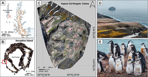
The topographic characteristics of the island make it an ideal location for the settlement of Chinstrap penguin colonies (Pygoscelis antarcticus) (Smith et al. 2003). In this case study, monitoring was carried out with remote sensing tools in the Vapor Col penguin colony (62 ° 59ʹS 60 ° 44ʹW) (Figure 1(c)), which is characterized by its ice-free surface and its abrupt slope on the southwest coast of the island, near Stonethrow Ridge. It is one of the biggest Chinstrap penguin colonies at Deception Island (population census of 19,177 breeding pairs of chinstrap penguin documented by Naveen et al. 2012), although a recess since the 1991 until 2008 is observed, evidencing a substantial decrease in their population as documented by (Barbosa et al. 1997, 2012).

Satellite imagery

Sentinel-2 (S2) and Landsat 8 (L8) imagery were the sources of imagery selected for comparison with the reflectance data obtained with the UAV-equipped multispectral sensor. The ease for users to access these public and high-quality data to carry out coastal environmental studies, as well as the similarity between the spectral bands between the different sensors considered, make these imagery sources ideal for the study presented here. However, it is interesting to emphasize the existence of other not-free or commercial imagery sources with higher spatial resolution that could improve the results obtained, such as PlanetScope or World-View imagery, but that have not been considered in this study due to their poor spectral and radiometric resolution.

• Sentinel-2 Level 1C (S2L1) and Sentinel-2 Level 2A (S2L2) top-of-atmospheric (TOA) products resampled at a 10 m spatial resolution were retrieved from the Copernicus Open Access Hub (https://scihub.copernicus.eu/), using the Sentinel-2 scene corresponding to 2 February 2021 (tile 20EPR), the date without cloud cover closest to the UAV surveys. The Level 2A processing includes the Sen2Cor atmospheric correction. Detailed information on the Sentinel-2 mission, multispectral instrument (MSI) and radiometric characteristics are provided in the User Handbook (ESA, 2015, 2017).

• Landsat 8. Orthorectified and atmospherically corrected Level 2 images at 30 m spatial resolution were retrieved from Earth Explorer (https://earthexplorer.usgs.gov/). The tile of study was in path 217 and row 104, and corresponded to 12 January 2021, also the date without cloud cover closest to the UAV surveys. Reflectance products were obtained using the Land Surface Reflectance Code (LaSRC) algorithm. Detailed information on the Landsat 8 mission is provided in Knight and Kvaran (2014).

UAV data collection

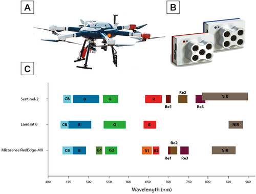
An UAV hexacopter with three-bladed propellers was used in this study (Condor, Dronetools ©, Figure 2(a)), which has a powered electric motor by four 7,000 mA Lithium-ion batteries (DJI6010). The equipment mounted on the UAV includes a multispectral camera to capture the images, the Micasense RedEdge-MX multispectral dual sensor (Figure 2(b)), which is capable of capturing spectral information with its 10 different channels (Figure 2(c)): blue (444 nm and 475 nm), green (531 nm and 560 nm), red (650 nm and 668 nm), red edge (705 nm, 717 nm and 740 nm) and near infrared (840 nm) wavelengths. The sensor includes its own positioning system and Downwelling Light Sensor (DLS) with built-in GPS, allowing the control of solar angle and light conditions during the flight. Radiometric calibration took place through the use of the included calibration panel (RP04-1,924,106-0B), which was captured before and after the UAV surveys. By using both the DLS and the calibration panel during the data collection, it is possible to obtain a high-quality reflectance map during the image processing.

Figure 2. (a) Condor hexacopter used in this research. (b) Micasense RedEdge-MX dual multispectral camera. (c) Sentinel-2, Landsat 8 and Micasense RedEdge-MX spectral bands comparison.

The UAV flight was carried out on 8 February 2021 in the Vapor Col penguin colony with meteorological conditions of almost entirely covered skies, at a constant flight height of 100 m achieving approximately 6.04 cm/pixel resolution in acquired imagery. Flight planning was carried out with DJI Ground Station Pro (Dà-Jiāng Innovations (DJI), Shenzhen, Guangdong, GSP v. 2.0.15) software and then uploaded to the UAV computer system. Seventy percent front and side overlaps were considered when setting up the flight plan. Simultaneously to the flights, photos and in situ samples were taken, allowing us the validation of the observations made with UAVs. We used the MicaSense’s own terrain following tool for the dual multispectral camera during the UAV survey in order to maintain the established flight plan parameters along the entire area. In addition, the Spanish civil aviation regulations (Spanish, Agency for Aviation Safety, AESA) were followed during all UAV operations.

The software Pix4D mapper (Pix4D SA, Lausanne, Switzerland) was used to process the multispectral images for the generation of the orthomosaics. The software creates an orthomosaic of the surface reflectance values in three recognized steps: i) initial processing (image alignment); ii) creation of a 3D point cloud; and iii) generation of the digital elevation model (DEM), reflectance orthomosaic and indices. Low light conditions made light sensor data, and therefore a calibration method that takes them into account, necessary. In the last processing step, the radiometric processing and calibration were performed using the method “Sun Irradiance and Sun Angle using DLS IMU.” As a result, a single orthomosaic of the surface reflectance ranging between 0.0 and 1.0 for each pixel were generated for each multispectral band (10 orthomosaics).

Image classification

In this study, the images obtained by remote sensing were classified from the spectral behavior of each land cover classes. The resolution provided by the sensor on board the UAV was even possible to differentiate between different types of vegetation (unidentified species in this study), soil, snow, guano and water. In order to do this, visual interpretation based on UAV images with high spatial resolution was performed, and then regions of interest (ROIs) were selected with the spectral information of each land cover class serving as a training file for the subsequent generation of thematic maps. Four different classification techniques (Support Vector Machine (SVM), Spectral Angle (SAC), Maximum Likelihood (MLC) and Random Forest (RFC)) were tested in UAV images to determine which of them works better for the classification of these systems. SVM is a machine learning algorithm that can deal with statistically unknown data derived of small training sets created from spectral data, and validated with in situ information (Vapnick 1995). With this algorithm, training data are mapped into a larger-dimensional space by applying kernel functions, where the different cover classes are linearly separed by the hyperplane between them (Miranda et al. 2020). The results reported by Miranda et al. (2020) suggested that the radial base function offers the best outcomes when working with spectrally complex ecosystems, so it was used as the transformation nucleus in this case study. One of the most commonly used thematic classifiers is the MLC that, assuming a Gaussian distribution, determines the likelihood that a pixel corresponds to a specific thematic class (Richards and Jia 2006; Román et al. 2021). SAC is an algorithm that determines the spectral similarity between a pixel spectrum and an existing reference spectra, based on the angular deviation between the two spectra, and assuming that they form two vectors in an n-dimensional space (Richards and Jia 2006; Román et al. 2021). RFC is an ensemble classifier that generates decision trees from a randomly selected subset of training samples and variables through replacement, so the same sample can be selected reiteratedly (Belgiu and Dragut 2016). We set two parameters for the generation of forest trees: the number of decision trees (Ntree), and the number of variables to be selected and tested (Mtry).

The training polygons were drawn manually by a single person, up to a total of 50 polygons of 1 m² maximum for each land cover training set. For the performance of the algorithms, the SAGA GIS software (Conrad et al. 2015) was used. All bands were used as input for each sensor when performing image classification (8 bands – from 443 to 842 nm – for S2, 5 bands – from 440 to 865 nm – for L8, and 10 bands – from 444 to 840 nm – for MicaSense RedEdge-MX data, according to Figure 2). The parameters used for each classification algorithm are summarized in Table 2.

Table 2. Input variables selected for each image classification algorithm in SAGA GIS software.

SVM	RF	MLC	SAC
Model Source: Create from polygons	Model Source: Create from polygons	Model Source: Create from polygons	Model Source: Create from polygons
Type: C-SVC	Number of Samples: 5000	Probability Threshold: 0	Spectral Angle Threshold: 0
Kernel: radial basis function	Number of trees: 100	Probability Reference: relative
Degree: 3	Minimum Sample Count: 2
nu-SVR: 0.5	Maximum Categories: 15
SVR Epsilon: 0.1	Regression Accuracy: 0.01
Cache Size: 100
Epsilon: 0.001

Once image classification was performed, the results were imported into the QGIS software to make them go through a sieving process that would allow cleaning of the classifications of the individual pixels (threshold: groups of 10 pixels) that correspond to misclassification errors, and for its graphical representation. To evaluate the efficiency of the algorithm to classify the ecosystem of Antarctic penguin colonies, error matrices were drawn up and statistical values such as the Cohen’s Kappa Index or Overall Accuracy were calculated, following Oloffson et al. (2014). This method makes a comparison between the thematic map generated and “real” maps from the generation of a stratified random sampling design. Overall Accuracy (OA) derives from the sum of the major diagonal divided by the total number of sample units in the error matrix (Congalton and Green 2009; Oloffson et al. 2014). If OA is above 80%, the results obtained could be considered as good and reliable. Regarding the Cohen’s Kappa Index, it is based on the difference between the actual agreement in the error matrix (e.g. the agreement between the remotely sensed classification and the reference data as indicated by the major diagonal) and the chance agreement that is indicated by the row and column totals (e.g. marginals). This index can take values between −1 and +1, being considered the better results the closer to +1 (Congalton and Green 2009). Finally, and in order to compare the different sensors, the mean reflectance value and the standard deviation of all the pixels corresponding to each land cover class were calculated according to the results obtained with the best classifier obtained. These values were represented in the spectral signature graphs, in which the wavelengths (nm) are on the x-axis and the reflectance (dimensionless between 0 and 1) is on the y-axis.

Spectral comparison

The UAV data at 6.04 cm/pixel size was resampled and aligned in QGIS to match the satellite pixel size of S2 at 10 m employing the bilinear interpolation method, using the georeferenced satellite image as a background. In order to compare both sensor datasets, five reflectance value areas (box of 10 × 10 m) for each class (vegetation, soil, snow and guano) were extracted from the UAV and S2 (L1 and L2). Since it is such a heterogeneous ecosystem, it is difficult to find pure pixels that only correspond to one class with S2 imagery, especially with guano and vegetation cover. However, central pixels of the class cover were selected whenever possible.

Red edge and NIR bands were used to define a threshold to isolate the guano patches of the colonies, since guano shows a higher reflectance in the NIR band in comparison with other bands (Bird et al. 2020; Fretwell et al. 2015). Moss spectral behavior is quite similar to vascular plants, where reflectance differences between species may be also exhibited in the NIR region. Green vegetation peaked around 690–740 nm, four to five times higher than that of soil (Calviño-Cancela and Martín-Herrero 2016; Sotille et al. 2020). Malenovský et al. (2015), (2017)) demonstrated that spectral signature of healthy moss differs from stressed moss, particularly between 650 and 780 nm, so we can find differences between moss classes with higher variability in the red edge region. Lichens show a weak absorption in the 685 nm, with more variability between lichen species in the visible and NIR regions (Calviño-Cancela and Martín-Herrero 2016; Sotille et al. 2020). Overall, vegetation shows high reflectance in infrared wavelengths and low reflectance in visible wavelengths, due to chlorophyll absorption and tissue cell structure (Sotille et al. 2020). There are some factors affecting bare soil reflectance that depends on the characteristics of the soil type (sand, rocks or pyroplasts), including moisture content, soil texture, surface roughness or presence of organic matter content. These factors influence soil reflectance, showing a high variability between sensors in the visible wavelengths and from 740 nm wavelengths (Lillesand and Kiefer 1999).

The correlation between the UAV and S2 data was evaluated band-by-band and pixel-by-pixel from the application of a linear regression model to the point cloud resulting from the representation of the reflectance values obtained in the extracted pixels, and of the calculation of the coefficient of determination (R²). To validate the consistency of both sensors, the band-by-band root mean square error (RMSE, Eq.1(1) $RMSE=\sqrt{\frac{{\sum }_{i=1}^n{\left(O_i-M_i\right)}^2}{n}}$(1) ), mean absolute error (MAE, Eq.2(2) $MAE=\frac{{\sum }_{i=1}^n\left|O_i-M_i\right|}{n}$(2) ), and bias (Eq.3)(3) $bias=\frac{{\sum }_{i=1}^n\left(O_i-M_i\right)}{n}$(3) between all the UAV resampled pixels and the corresponding S2 data was calculated.

(1) $RMSE=\sqrt{\frac{{\sum }_{i=1}^n{\left(O_i-M_i\right)}^2}{n}}$(1)

(2) $MAE=\frac{{\sum }_{i=1}^n\left|O_i-M_i\right|}{n}$(2)

(3) $bias=\frac{{\sum }_{i=1}^n\left(O_i-M_i\right)}{n}$(3)

where i represents each classification cover class, Mi represents the UAV data considered as reference value, Oi represents the S2 data and n is the sample size (n = 20) (Seegers et al. 2018).

Results

Image classification

All the algorithms tested in this study (Figure 3) performed well for the generation of thematic maps in the Vapor Col penguin colony, obtaining Overall Accuracy (OA) values above 80% in all cases. However, the best results were obtained with non-parametric machine learning classifiers, SVM (93.19% OA and 0.78 Cohen’s Kappa Index) and RFC (90.83% OA and 0.85 Cohen’s Kappa Index).

Figure 3. Zoom of the Vapor Col penguin colony. MLC, SAC, RFC and SVM algorithms were applied to make the supervised classifications showed in the figure.

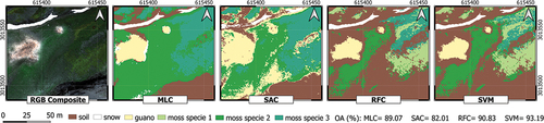
Table 3 shows the statistical parameters obtained after the accuracy assessment of the four machine learning algorithms used for image classification, OA and Cohen’s Kappa index. Producer and user accuracies are also displayed in the table (Oloffson et al. 2014). Soil and snow were the thematic classes more accurately classified with higher user and producer accuracies, while the moss cover species were the surface classes prone to confusion with the lowest producer accuracy values among all thematic classes. Regarding the values of the Cohen’s Kappa index, the two non-parametric machine learning classifiers also obtained the highest values (0.88 SVM and 0.85 RFC) compared to the other two algorithms (0.77 MLC and 0.62 SAC), highlighting a high agreement between the generated classes in all cases.

Table 3. Accuracy Assessment of thematic maps generated from UAV imagery using the four algorithms tested in this study (MLC, SAC, SVM and RFC), including user accuracy (“U-acc”), producer accuracy (“P-acc”), the OA (%) and the Cohen’s Kappa index.

Class	SVM		RFC		MLC		SAC
	U-acc	P-acc	U-acc	P-acc	U-acc	P-acc	U-acc	P-acc
Soil	94.71	97.84	90.35	95.52	99.27	88.89	95.02	85.93
Snow	98.92	82.94	98.89	68.78	87.15	99.95	95.06	45.98
Guano	78.86	99.96	79.51	99.96	77.22	98.89	76.38	98.46
Moss specie 1	86.73	78.67	95.12	29.47	82.31	40.23	76.24	60.35
Moss specie 2	89.69	49.61	94.81	34.27	77.44	77.44	75.01	63.21
Moss specie 3	92.68	27.50	92.47	97.96	48.36	48.37	49.73	78.68
Overal Accuracy (%)	93.19		90.83		89.07		82.01
Cohen’s Kappa	0.88		0.85		0.77		0.62

SVM classification was generated for each sensor from the training regions created from the information obtained in situ in the study area (Figure 4). Higher Overall Accuracy and Cohen’s Kappa index values indicated that higher resolution UAV images yielded higher precision than lower resolution satellite images. For this reason, the most accurate SVM was performed with the multispectral camera mounted on UAV, which presented values of 93.19% OA and of 0.88 in the Cohen’s Kappa index, followed by S2L2 (87.26% OA and Cohen’s Kappa of 0.73), L8L2 (70.77% OA and Cohen’s Kappa of 0.53) and lastly of S2L1 (65.97% OA and Cohen’s Kappa of 0.52). The lower classification accuracy associated to L8L2 data is probably due to the higher hetereogenity holded in a 30 m L8 pixel compared to a 10 m S2 pixel or a centimetric UAV pixel. It might also be due to the atmospheric signals (water vapor, aerosols, sea fog, between others) that still remain in the data after reprocessing (see Materials and Methods Section for more information).

Figure 4. SVM thematic maps obtained from the UAV, S2 (L1 and L2) and L8L2 imagery, with three highlighted regions of interest. In S2 (L1 and L2) and L8L2 RGB composite images, the area covered by the UAV in Vapor Col is indicated in yellow. Dates: UAV (8 February 2021), S2 (2 February 2021) and L8L2 (12 January 2021).

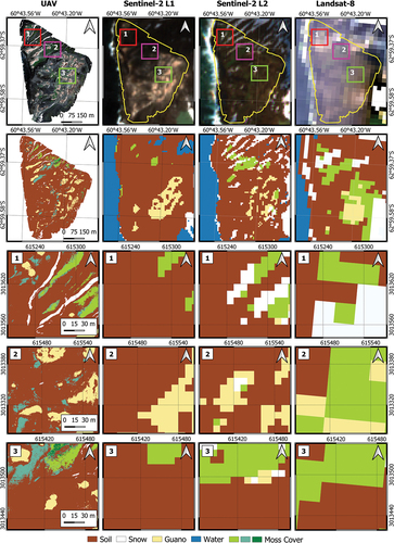
In general terms, and from the information provided by UAV data, in the Vapor Col penguin colony the most extensive land cover class was soil (212,591 m²), followed by the guano patches corresponding to the breeding sites (19,995 m²). With the Micasense RedEdge-MX dual multispectral sensor it has not only been possible to specify the coverage of the classes specified in this study with a centimetric level of detail, but also to differentiate between different types of vegetation, which as a whole (15,229 m²) did not exceed the extent of the cover classified as guano. In the S2L2 thematic map, soil was still the dominant cover, although vegetation (20,300 m²) and guano (20,500 m²) cover were similar. In addition, reflectance values were higher than those obtained with the sensor mounted in the UAV, and they did not allow differentiation between vegetation classes. However, if compared with the supervised analysis generated with the S2L1 data, it could be seen how it made important classification errors, presenting a land cover of 506,900 m², as well as guano and vegetation covers of 37,200 m² and 6,100 m² respectively. With L8L2, the vegetation (26,100 m²) and guano (81,900 m²) covers were not precise enough, and as with S2, it was not possible to differentiate between vegetation classes. It is important to emphasize that these results may be influenced by the existing temporal difference in the data of each of the sensors, since between UAV and S2 the difference is 6 days while between UAV and L8 the difference is 1 month. However, only changes in the snow cover could be perceptible in such a short interval between the data, since the area of guano and vegetation of the penguin colonies remains stable in this period of time that it also coincides with the Austral Summer where the snowfalls are less intense.

Spectral signature analysis

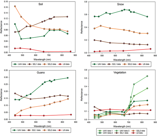
The UAV and satellite sensors reflectance spectra for each coverage class (soil, snow, guano and vegetation) are shown in Figure 5 Based on the general spectrum shape, S2L2 data appeared to show better agreement with UAV data than S2L1 and L8L2. For these two sensors (UAV and S2L2) in the four classes of substrate represented, there seemed to be more pronounced differences in the spectral curve from 700 nm, coinciding with the Red Edge and NIR bands, while the values of reflectance were more consistent in the visible part of the spectrum. Snow, guano and vegetation profiles had a good match between sensors, showing a similar spectral signature in all cases. However, there were bigger differences between sensors when analyzing soil profiles, probably due to the variability introduced at each pixel when considering the different soil types (rocks, sand and pyroplasts) as a single land cover class.

Figure 5. Land cover classes reflectance spectrum for each sensor (UAV, S2 (L1 and L2) and L8L2). It should be noted that in the case of the UAV, the vegetation substrate has three different classes. Wavelength (nm) is represented in the x-axis and reflectance (dimensionless) is represented in the y-axis.

Band-by-band and pixel-by-pixel comparison

Figure 6 shows the linear regression models corresponding to the band-by-band and pixel-by-pixel comparison between the UAV multispectral data resampled to 10 m and the S2L2 data, indicating that S2L2 data had good fitting to UAV with relatively high coefficient of determination (R²) values especially in the green-560 nm (R² = 0.80), blue-475 nm (R² = 0.79), red-668 nm (R² = 0.74), rededge-705 nm (R² = 0.64) and NIR-840 nm (R² = 0.63) bands. However, the rededge-740 nm band had a weaker relationship, presenting the lowest R² value (R² = 0.55). The linear regression models that resulted from comparing the UAV data with those of S2L1 are also shown in Figure 6, with minimal R² values, which indicated the poor fitting between the data, and highlighted the need for precise atmospheric correction methods for accurate performance of the SVM in these complex polar coastal areas. Results showed that the UAV and satellite data followed the same trend, although obviously the downscaling applied to UAV data increased the interpixel variability in the reflectance values.

Figure 6. Pixel-by-pixel and band-by-band comparison of UAV surface reflectance data with S2 Level 2 atmospherically corrected product data (triangles) and with S2 Level 1 orthoimage product data (circles). Twenty pixels (n = 20) were selected in four different types of substrate: snow (gray color), guano (brownish color), soil (dark brown color) and vegetation (green color).

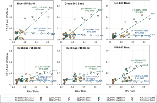
To assess the consistency of both sensors, Table 4 shows the statistical spectral analysis applied: R², RMSE, MAE and bias. As with R², it can be observed that for all bands the S2L2 values were closer to the UAV data than those of S2L1, as indicated by lower RMSE and MAE. In all cases, the negative values of the bias estimation indicated satellite data underestimated reflectance compared to the UAV data. However, the values were close to 0 with minimal differences between the data, and in all cases better for S2L2 (except in the blue-475 nm band, which is very similar). It should be noted that surface reflectance data of the UAV was always higher than those from satellites, except for the bright pixels selected in areas covered by snow so that the five points located in the snow had positive bias values for all bands, indicating an overestimation of the reflectance values.

Table 4. Statistics calculated (R², RMSE, MAE and bias) for the linear regression models applied to the relationships between the multispectral sensor equipped in the UAV and S2 (L1 vs L2) for comparison.

		R^2	RMSE	MAE	bias
Blue-475 nm Band	L1	0.07	0.17	0.11	−0.03
	L2	0.79	0.09	0.06	−0.04
Green-560 nm Band	L1	0.06	0.20	0.12	−0.09
	L2	0.80	0.09	0.07	−0.06
Red-668 nm Band	L1	0.01	0.24	0.15	−0.14
	L2	0.74	0.14	0.10	−0.10
RedEdge-705 nm Band	L1	0.01	0.24	0.17	−0.16
	L2	0.64	0.19	0.14	−0.14
RedEdge-740 nm Band	L1	0.03	0.25	0.19	−0.18
	L2	0.55	0.19	0.15	−0.14
NIR-840 nm Band	L1	0.04	0.25	0.20	−0.19
	L2	0.63	0.13	0.10	−0.10

Discussion

UAVs for penguin colony ecosystem characterization

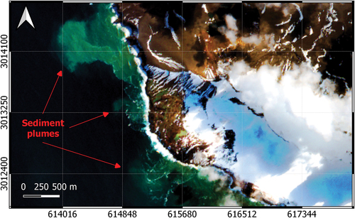
This study shows that high-quality data can be obtained from an UAV at 100 m altitude in an ecosystem in which the typical extreme conditions of maritime Antarctica render traditional field surveys very risky and difficult. In addition, it represents the first approximation in m² of the guano cover of an Antarctic penguin colony on Deception Island. This is a fundamental piece of data to determine the inputs of important bioactive metals (e.g. Cu, Fe, Mn, Zn) that can take place toward the surface waters of the sea (Figure 7), since penguin guano plumes have been suggested as an important source of these metals to the ocean (Shatova et al. 2016; Sparaventi et al. 2021).

Figure 7. Sentinel-2 L2 true color composition on 2 February 2021, in which sediment plumes have been pointed out with red arrows.

Antarctic flora distribution and speciation could also be influenced by the location of these guano patches in the colony, since our results show how the vegetation tends to grow around the areas covered by guano, acting as a source of nutrients and metals (Tovar-Sánchez et al. 2021). This tool also allows us to obtain data with enough precision to characterize the spatial and spectral variability of the typical lichen and moss communities of the Antarctic tundra, providing a noninvasive method to analyze environmental changes in their micro-topography and physiological state (Lucieer, Robinson, and Turner 2011; Lucieer et al. 2014a; Malenovský et al. 2015, 2017; Turner et al. 2014, 2018; Zmarz et al. 2018).

Image classification performance

The four algorithms tested with UAV imagery yielded accurate and reliable results, with the SVM algorithm providing the most accurate results (93.19% OA and 0.78 Cohen’s Kappa Index). With the SVM algorithm, user and producer accuracies show values above 70% in all cover classes except in vegetation where these values are especially lower in producer accuracies. This reflects that classification performance could be improved, in particular with the moss cover classes, where small misclassification could be mainly related to the spectral similarity between vegetation species. Several studies suggested that SVM is the best classifier when using a small number of training samples (e.g. Foody and Mathur 2004; Mountrakis, Im, and Ogole 2011; Rupasinghe et al. 2018), as in this case study. For example, Miranda et al. (2020) successfully apply the SVM algorithm to carry out spatio-temporal monitoring of the vegetation covers of ice-free areas in Antarctica with UAV and satellite imagery, demonstrating that they can provide information that quantitatively describes the evolution of these ecosystems. That is why we use the SVM algorithm for the spectral comparison between remote sensing techniques, since it offers the most robust results.

The UAV’s centimeter-scale spatial resolution helps the information contained in each pixel to be more precise than that contained in a pixel of S2 at 10 m or a pixel of L8 at 30 m, which stores a more heterogeneous amount of information among the different land cover classes. In this way, UAV data have the potential to not only specify the extent and location of each of the classes, but also to distinguish between different species of vegetation. However, the accuracy assessment carried out on each thematic map reflects that the S2L2 data do not differ so much from those of UAV for the generation of thematic maps in this type of coastal ecosystems (93.82% OA with UAV versus 87.26% OA with S2L2). In addition, the extent of the vegetation and especially guano covers resulting from this analysis are quite similar between UAV and S2L2, so the S2L2 data could be used to make precise estimates of the amount of guano in the coastal colonies of Antarctic penguins. This could not be possible with the data from L8L2 or S2L1, which provided much less accurate results for penguin colony size studies, as demonstrated in other research using Landsat data to map Adélie penguin colonies (Lynch and Schwaller 2014; Schwaller, Southwell, and Emmerson 2013). These studies confirmed that Landsat retrievals performed better for continental or regional-scale studies than in situ observations, although UAV and S2L2 data are more accurate for local studies carried out in these characteristic Antarctic ecosystems.

Spectral signature analysis

We evaluated the reflectance spectra of the four main land cover classes classified in our study area (soil, snow, guano, and vegetation). The L8L2 reflectance spectra for each substrate show little variability in the curve due to the lower spatial resolution of the data. However, similar trends are found between UAV and S2 data (Level 1 and 2). The vegetation spectral curve shows a similar behavior for UAV and S2, with absorption minima in red and blue, and with reflectance peaks especially in the NIR. The same happens with the spectral curve of the snow, where there is a slight difference between the UAV and S2 associated with the presence of shadows in the satellite images. These profiles show that guano has a high reflectance in red bands in comparison with other cover classes, which allows it to be differentiated from most types of vegetation. Several authors who have previously mapped guano with satellite imagery (Brown 2018; Fretwell et al. 2015; Schwaller, Benninghoff, and Olson 1984; Schwaller, Southwell, and Emmerson 2013), use the distinctive behavior of guano spectral signature in the (SWIR) bands. In this comparative study, we ignore the SWIR part of the spectrum despite its importance, since MicaSense RedEdge-MX dual sensor only uses NIR bands in addition to standard RGB bands. Furthermore, we offer a reliable and precise formula for monitoring guano from the spectral information derived from the red and NIR bands, without the need for specialized hyperspectral equipment. Fretwell et al. (2015) compared the spectral signature of guano with information from other public spectral libraries, concluding that guano presents a unique characteristic spectral signature with peaks also in the red and NIR bands. It is therefore ideal for future studies to apply the spectral information derived from the cover classes classified in this study to other regions of Antarctica, so that it would be possible to generate an index or a tool that would allow rapid, efficient and simple estimation of the extent of the guano patches typical of the Antarctic penguin colonies as long as radiometer measurements are taken in situ to validate the results.

Band-by-band and pixel-by-pixel comparison

Spatial downscaling applied to UAV data from 6.04 cm to 10 m to match the satellite resolution provided reflectance values consistent with those obtained with S2L2. According to the statistics obtained, S2L2 data are more similar to the UAV data than S2L1. This highlights the need to carry out an atmospheric correction on the satellite data, since the radiance reaching the sensor interacts with the atmosphere and can be affected by various parameters such as aerosols, Rayleigh, scattering, water vapor, among others. In this study, Sen2Cor is the processor applied to TOA Level 1C orthoimage product for atmospheric correction, obtaining a good performance when comparing with UAV data. Previous studies with Sentinel-2 imagery in complex coastal and inland waters have obtained consistent results using the Sen2Cor processor (e.g. Kutser et al. 2018; Pereira-Sandoval et al. 2019; Qing et al. 2021; Sobel, Kiaghadi, and Rifai 2020), although it also proves to be more effective for studies in terrestrial coastal ecosystems (e.g. Marzialetti et al. 2019; Pham et al. 2019; Villa et al. 2021).

However, despite the strong correlation in the visible bands between UAV and S2L2 data, a significant difference in reflectance was found in red edge and NIR bands. These differences between sensors arise as a result of various factors, such as the radiometric and atmospheric correction, signal-to-noise ratio, the spatial resolution of the sensors, the temporal difference between UAV and satellite data or the band width of the sensors (Sozzi et al. 2020; Zabala 2017). Other studies have found good agreement between UAV mounted multispectral sensors and S2L2 data, such as Castro et al. (2020) who tested the correlation between both tools in a eutrophicated water reservoir to develop a multi-scale monitoring tool, or Zabala (2017), who also used the same tools for the monitoring of a crop environment obtaining a significant difference in reflectance values, as in our research.

Conclusions

Our results demonstrate that a UAV-mounted multispectral camera allowed us to obtain high-quality images for monitoring the key elements of the Antarctic penguin colonies ecosystem from their unique and characteristic spectral signatures. In fact, these spectral signatures can provide very valuable information for the generation of a tool that allows this methodology to be applied in an automated manner in other case studies, producing precise maps of the flora and landforms of Antarctica. It would be also interesting to use these high-quality UAV images to accurately count the number of penguins in the colonies, constituting a less intrusive and even more precise methodology than traditional in situ censuses. In addition, guano cover estimations can be used in order to determine the number of penguin breeding pairs per m² of coverage in each colony, or to quantify its influence in moss/lichens coverage growing due to the inputs of important bioactive metals and nutrients from guano. This study evidenced the effectiveness of non-parametric machine learning algorithms for the generation of thematic maps, being the SVM the algorithm that best adapts to the spectral characteristics of the Antarctic ecosystem. In addition, it is shown that the higher spatial resolution of UAV data improved the precision compared to the satellite results, although S2L2 data also allowed the generation of accurate local thematic maps of Antarctic penguin colonies covering larger areas than those covered by an UAV. In contrast, the 30 m spatial resolution of L8 was insufficient to accurately characterize the different elements of this highly heterogeneous ecosystem. This study also tested the compatibility of UAV data with S2 level 1 and level 2 (data after the Sen2Cor atmospheric correction). The results highlighted the need to correct the S2 level 1 data to eliminate the atmospheric interferences and residuals, resulting in an improvement in the overall accuracy of the satellite’s surface reflectance values. UAVs complement the shortcomings of satellite remote sensing in order to take a further step in the study of polar regions under the scenario of global climate change.

Acknowledgements

The authors thank the military staff of the Spanish Antarctic Base Gabriel de Castilla, the crew of the Sarmiento de Gamboa oceanographic vessel and the Marine Technology Unit (UTM-CSIC) for their logistic support, without which the XXXIV Spanish Antarctic campaign and this research would not have been possible. We also thank all the team members of OPECAM and SEADRON, Antonio Moreno and David Roque, for their technical support with the UAV operations. The authors would like to thank the European Space Agency, the European Commission and the Copernicus programme for distributing Sentinel-2 imagery as well as the United States Geological Survey (USGS) and the National Aeronautics and Space Administration (NASA) for distributing Landsat-8 data. We also thank Martha B. Dunbar, from the ICMAN-CSIC, for her English language edits.

Disclosure statement

No potential conflict of interest was reported by the author(s).

Data Availability Statement

The authors confirm that the data supporting the findings of this study are available within the article [and/or] its supplementary materials.

Additional information

Funding

This research was funded by grants/projects RTI2018-098048-B-100 (PiMetAn), EQC2018-004275-P, EQC2019-005721, RTI2018-098784-J-I00 and IJC2019-039382-I funded by MCIN/AEI/ 10.13039/501100011033 and by “ERDF A way of making Europe.” A. Román is supported by grant FPU19/04557 funded by Ministry of Universities of the Spanish Government. This work represents a contribution to CSIC Thematic Interdisciplinary Platforms POLARCSIC and PTI TELEDETECT.

References

- Ancel, A., R. Cristofari, P. N. Trathan, C. Gilbert, P. T. Fretwell, and M. Beaulieu. 2017. “Looking for New Emperor Penguin Colonies? Filling the Gaps.” Global Ecology and Conservation 9: 171–179. doi:10.1016/j.gecco.2017.01.003.
- Angulo-Preckler, C., P. Pernet, C. García-Hernández, G. Kereszturi, A. M. Álvarez-Valero, J. Hopfenblatt, M. Gómez-Ballesteros, et al. 2021. “Volcanism and Rapid Sedimentation Affect the Benthic Communities of Deception Island, Antarctica”. Continental Shelf Research 220: 104404. doi:10.1016/j.csr.2021.104404.
- Atkinson, A., S. L. Hill, E. A. Pakhomov, V. Siegel, C. S. Reiss, V. J. Loeb, D. K. Steinberg, et al. 2019. “Krill (Euphasia Superba) Distribution Contracts Southward during Rapid Regional Warming.” Nature Climate Change 9: 142–147. doi:10.1038/s41558-018-0370-z.
- Barbosa, A., J. Moreno, J. Potti, and S. Merino. 1997. “Breeding Group Size, Nest Position and Breeding Success in the Chinstrap Penguin.” Polar Biology 18: 410–414. doi:10.1007/s003000050207.
- Barbosa, A., J. Benzal, A. De León, and J. Moreno. 2012. “Population Decline of Chinstrap Penguins (Pygoscelis Antarctica) on Deception Island, South Shetlands, Antarctica.” Polar Biology 35: 1453–1457. doi:10.1007/s00300-012-1196-1.
- Belgiu, M., and L. Dragut. 2016. “Random Forest in Remote Sensing: A Review of Applications and Future Directions.” ISPRS Journal of Photogrammetry and Remote Sensing 114: 24–31. doi:10.1016/j.isprsjprs.2016.01.011.
- Bird, C. N., A. H. Dawn, J. Dale, and D. W. Johnston. 2020. “A Semi-Automated Method for Estimating Adélie Penguin Colony Abundance from A Fusion of Multispectral and Thermal Imagery Collected with Unoccupied Aircraft Systems.” Remote Sensing 12: 3692. doi:10.3390/rs12223692.
- Bricher, P. K., A. Lucieer, and E. Woehler. 2008. “Population Trends of Adélie Penguin (Pygoscelis Adeliae) Breeding Colonies: A Spatial Analysis of the Effects of Snow Accumulation and Human Activities.” Polar Biology 31: 1397–1407. doi:10.1007/s00300-008-0479-z.
- Brown, J. A. 2018. “Remote Sensing of Penguin Populations: Development and Application of a satellite-based Method.” Doctoral Thesis in Philosophy, University of Cambridge.
- Calviño-Cancela, M., and J. Martín-Herrero. 2016. “Spectral Discrimination of Vegetation Classes in Ice-Free Areas of Antarctica.” Remote Sensing 8: 856. doi:10.3390/rs8100856.
- Castro, C. C., J. A. D. Gómez, J. D. Martín, B. A. H. Sánchez, J. L. C. Arango, F. A. C. Tuya, and R. Díaz-Varela. 2020. “An UAV and Satellite Multispectral Data Approach to Monitor Water Quality in Small Reservoirs.” Remote Sensing 12 (9): 1514. doi:10.3390/rs12091514.
- Clucas, G. V., M. J. Dunn, G. Dyke, S. D. Emslie, H. Levy, R. Naveen, M. J. Polito, O. G. Pybus, A. D. Rogers, and T. Hart. 2014. “A Reversal of Fortunes: Climate Change ‘Winners’ and ‘Losers’ in Antarctic Peninsula Penguins.” Scientific Reports 4: 5024. doi:10.1038/srep05024.
- Congalton, R., and K. Green. 2009. Assessing the Accuracy of Remotely Sensed Data: Principles and Practices. 2nd ed. Boca Raton: CRC/Taylor & Francis.
- Conrad, O., B. Bechtel, M. Bock, H. Dietrich, E. Fischer, L. Gerlitz, J. Wehberg, V. Wichmann, and J. Böhner. 2015. “System for Automated Geoscientific Analyses (SAGA) V. 2.1.4.” Geoscientific Model Development 8 (7): 1991–2007. doi:10.5194/gmd-8-1991-2015.
- Duarte, B., C. Gameiro, A. R. Matos, A. Figueiredo, M. Sousa, C. Cordeiro, I. Caçador, P. Reis-Santos, V. Fonseca, and M. T. Cabrita. 2021. “First Screening of Biocides, Persistent Organic Pollutants, Pharmaceutical and Personal Care Products in Antarctic Phytoplankton from Deception Island by FT-ICR-MS.” Chemosphere 274: 129860. doi:10.1016/j.chemosphere.2021.129860.
- Dunn, M. J., J. A. Jackson, S. Adlard, A. S. Lynnes, D. R. Briggs, D. Fox, and C. M. Waluda. 2016. “Population Size and Decadal Trends of Three Penguin Species Nesting at Signy Island, South Orkney Islands.” PLoS ONE 11(10): e0164025. doi:10.1371/journal.pone.0164025.
- Dunn, M. J., S. Adlard, A. P. Taylor, A. G. Wood, P. N. Trathan, and N. Ratcliffe. 2021. “Un-crewed Aerial Vehicle Population Survey of Three Sympatrically Breeding Seabird Species at Signy Island, South Orkney Islands.” Polar Biology 44: 717–727. doi:10.1007/s00300-021-02831-6.
- European Space Agency. 2015. Sentinel-2 User Handbook, ESA Standard Document Paris, France: European Space Agency. https://sentinel.esa.int/documents/247904/685211/Sentinel-2_User__Handbook_ed
- European Space Agency, 2017. “Sentinel-2 MSI Technical Guide.” https://earth.esa.int/web/sentinel/technicalguides/sentinel-2-msi
- Foody, G. M., and A. Mathur. 2004. “Toward Intelligent Training of Supervised Image Classifications: Directing Training Data Acquisition for SVM Classification.” Remote Sensing of Environment 93: 107–117. doi:10.1016/j.rse.2004.06.017.
- Forcada, J., P. N. Trathan, K. Reid, E. J. Murphy, and J. P. Croxall. 2006. “Contrasting Population Changes in Sympatric Penguin Species in Association with Climate Warming.” Global Change Biology 12: 411–423. doi:10.1111/j.1365-2486.2006.01108.x.
- Fretwell, P. T., and P. N. Trathan. 2009. “Penguins from Space: Faecal Stains Reveal the Location of Emperor Penguin Colonies.” Global Ecology and Biogeography 18: 543–552. doi:10.1111/j.1466-8238.2009.00467.x.
- Fretwell, P. T., R. A. Phillips, M. Brooke, A. H. Fleming, and A. McArthur. 2015. “Using the Unique Spectral Signature of Guano to Identify Unknown Seabird Colonies.” Remote Sensing of Environment 156: 448–456. doi:10.1016/j.rse.2014.10.011.
- Fretwell, P. T., and P. N. Trathan. 2020. “Discovery of New Colonies by Sentinel2 Reveals Good and Bad News for Emperor Penguins.” Remote Sensing in Ecology and Conservation 7(2): 139–152. doi:10.1002/rse2.176 .
- Hodgson, J. C., R. Mott, S. Baylis, T. Pham, S. Wotherspoon, A. Kilpatrick, R. Raja Segaran, I. Reid, A. Terauds, and L. Koh. 2018. “Drones Count Wildlife More Accu- Rately and Precisely than Humans.” Methods in Ecology and Evolution 9: 1160–1167. doi:10.1111/2041-210X.12974.
- Huang, J., L. Sun, W. Huang, X. Wang, and Y. Wang. 2010. “The Ecosystem Evolution of Penguin Colonies in the past 8,500 Years on Vestfold Hills, East Antarctica.” Polar Biology 33: 1399–1406. doi:10.1007/s00300-010-0832-x.
- Ibáñez, J. M., J. Almendros, E. Carmona, C. Martínez-Arévalo, and M. Abril. 2003. “The Recent seismo-volcanic Activity at Deception Island Volcano.” Deep-Sea Research II 50: 1611–1629. doi:10.1016/S0967-0645(03)00082-1.
- Jerez, S., M. Motas, J. Benzal, J. Diaz, and A. Barbosa. 2013. “Monitoring Trace Elements in Antarctic Penguin Chicks from South Shetland Islands, Antarctica.” Marine Pollution Bulletin 69: 67–75. doi:10.1016/j.marpolbul.2013.01.004.
- Kattenborn, T., J. Lopatin, M. Förster, A. C. Braun, and F. E. Fassnacht. 2019. “UAV Data as Alternative to Field Sampling to Map Woody Invasive Species Based on Combined Sentinel-1 and Sentinel-2 Data.” Remote Sensing of Environment 227: 61–73. doi:10.1016/j.rse.2019.03.025.
- Kawaguchi, S., A. Ishida, R. King, B. Raymond, N. Waller, A. Constable, S. Nicol, M. Wakita, and A. Ishimatsu. 2013. “Risk Maps for Antarctic Krill under Projected Southern Ocean Acidification.” Nature Climate Change 3: 843–847. doi:10.1038/nclimate1937.
- Knight, E. J., and G. Kvaran. 2014. “Landsat-8 Operational Land Imager Design, Characterization and Performance.” Remote Sensing 6 (11): 10286–10305. doi:10.3390/rs61110286.
- Kokubun, N., W. Y. Lee, J. H. Kim, and A. Takahashi. 2015. “Chinstrap Penguin Foraging Area Associated with a Seamount in Bransfield Strait, Antarctica.” Polar Science 9: 393–400. doi:10.1016/j.polar.2015.10.001.
- Korczak-Abshire, M., A. Zmarz, M. Rodzewicz, M. Kycko, I. Karsznia, and K. J. Chwedorzewska. 2019. “Study of Fauna Population Changes on Penguin Island and Turret Point Oasis (King George Island, Antarctica) Using an Unmanned Aerial Vehicle.” Polar Biology 42: 217–224. doi:10.1007/s00300-018-2379-1.
- Kutser, T., B. Paavel, K. Kaljurand, M. Ligi, and M. Randla. 2018. “Mapping Shallow Waters of the Baltic Sea with Sentinel-2 Imagery.” 2018 IEEE/OES Baltic International Symposium (BALTIC), Klaipeda, Lithuania, 12-15 June 2018. doi:10.1109/BALTIC.2018.8634850
- LaRue, M. A., H. J. Lynch, P. O. B. Lyver, K. Barton, D. G. Ainley, A. Pollard, W. R. Fraser, and G. Ballard. 2014. “A Method for Estimating Colony Sizes of Adélie Penguins Using Remote Sensing Imagery.” Polar Biology 37: 507–517. doi:10.1007/s00300-014-1451-8.
- Lillesand, T. M., and R. W. Kiefer. 1999. Remote Sensing and Image Interpretation. Hoboken, New Jersey: John Wiley & Sons, Inc.
- Liu, K., W. Shi, and H. Zhang. 2011. “A Fuzzy topology-based Maximum Likelihood Classification.” ISPRS Journal of Photogrammetry and Remote Sensing 66: 103–114. doi:10.1016/j.isprsjprs.2010.09.007.
- Lucieer, A., A. Robinson, and D. Turner 2011. “Unmanned Aerial Vehicle (UAV) Remote Sensing for Hyperspatial Terrain Mapping of Antarctic Moss Beds Based on Structure from Motion (Sfm) Point Clouds.” 34th International Symposium on Remote Sensing of Environment, 10-15 April 2011, Sydney, Australia.
- Lucieer, A., D. Turner, D. H. King, and S. A. Robinson. 2014a. “Using an Unmanned Aerial Vehicle (UAV) to Capture micro-topography of Antarctic Moss Beds.” International Journal of Applied Earth Observation and Geoinformation 27: 53–62. doi:10.1016/j.jag.2013.05.011.
- Lucieer, A., Z. Malenovský, T. Veness, and L. Wallace. 2014b. “HyperUAS—Imaging Spectroscopy from a Multirotor Unmanned Aircraft System.” Journal of Field Robotics 31: 571–590. doi:10.1002/rob.21508.
- Lynch, H. J., and M. R. Schwaller. 2014. “Mapping the Abundance and Distribution of Adélie Penguins Using Landsat-7: First Steps Towards an Integrated Multi-Sensor Pipeline for Tracking Populations at the Continental Scale.” PLoS ONE 9: e113301. doi:10.1371/journal.pone.0113301.
- Lynch, H. J., R. White, R. Naveen, A. Black, M. S. Meixler, and W. F. Fagan. 2016. “In Stark Contrast to Widespread Declines along the Scotia Arc, a Survey of the South Sandwich Islands Finds a Robust Seabird Community.” Polar Biology 39: 1–11. doi:10.1007/s00300-015-1886-6.
- Lynch, M., C. Youngflesh, N. M. Agha, M. A. Ottinger, and H. J. Lynch. 2019. “Tourism and Stress Hormone Measures in Gentoo Penguins on the Antarctic Peninsula.” Polar Biology 42: 1299–1306. doi:10.1007/s00300-019-02518-z.
- Malenovský, Z., J. Turnbull, A. Lucieer, and S. Robinson. 2015. “Antarctic Moss Stress Assessment Based on Chlorophyll Content and Leaf Density Retrieved from Imaging Spectroscopy Data.” New Phytologist 208: 608–625. doi:10.1111/nph.13524.
- Malenovský, Z., A. Lucieer, D. H. King, J. D. Turnbull, and S. A. Robinson. 2017. “Unmanned Aircraft System Advances Health Mapping of Fragile Polar Vegetation.” Methods in Ecology and Evolution 8: 1842–1857. doi:10.1111/2041-210X.12833.
- Marzialetti, F., S. Giulio, M. Malavasi, M. G. Sperandii, A. T. R. Acosta, and M. L. Carranza. 2019. “Capturing Coastal Dune Natural Vegetation Types Using a Phenology-Based Mapping Approach: The Potential of Sentinel-2.” Remote Sensing 11 (12): 1506. doi:10.3390/rs11121506.
- Miranda, V., P. Pina, S. Heleno, G. Vieira, C. Mora, and C. E. G. R. Schaefer. 2020. “Monitoring Recent Changes of Vegetation in Fildes Peninsula (King George Island, Antarctica) through Satellite Imagery Guided by UAV Surveys.” Science of the Total Environment 704: 135295. doi:10.1016/j.scitotenv.2019.135295.
- Mountrakis, G., J. Im, and C. Ogole. 2011. “Support Vector Machines in Remote Sensing: A Review.” ISPRS Journal of Photogrammetry and Remote Sensing 66: 247–259. doi:10.1016/j.isprsjprs.2010.11.001.
- Mustafa, O., J. Esefeld, H. Gramer, J. Maercker, M. C. Rummler, and C. Pfeifer. 2017. “Monitoring Penguin Colonies in the Antarctic Using Remote Sensing Data .” In TEXTE 30/2017 Environmental Research of the Federal Ministry for the Environment, Nature Conservation, Building and Nuclear Safety (Jena, Germany) (Vol. 163, pp. 1862-4804). Dessau-Roßlau, Germany: Umweltbundesamt.
- Naveen, R., H. J. Lynch, S. Forrest, T. Mueller, and M. Polito. 2012. “First Direct, site-wide Penguin Survey at Deception Island, Antarctica, Suggests Significant Declines in Breeding Chinstrap Penguins.” Polar Biology 35: 1879–1888.
- Oloffson, P., G. M. Foody, M. Herold, S. V. Stehman, C. E. Woodcock, and M. A. Wulder. 2014. “Good Practices for Estimating Area and Assessing Accuracy of Land Change.” Remote Sensing of Environment 148: 42–57. doi:10.1016/j.rse.2014.02.015.
- Pereira-Sandoval, M., A. Ruescas, P. Urrego, A. Ruiz-Verdú, J. Delegido, C. Tenjo, X. Soria-Perpinyà, E. Vicente, J. Soria, and J. Moreno. 2019. “Evaluation of Atmospheric Correction Algorithms over Spanish Inland Waters for Sentinel-2 Multi Spectral Imagery Data.” Remote Sensing 11 (12): 1469. doi:10.3390/rs11121469.
- Pfeifer, C., A. Barbosa, O. Mustafa, H. U. Peter, M. C. Rümmler, and A. Brenning. 2019. “Using Fixed-Wing UAV for Detecting and Mapping the Distribution and Abundance of Penguins on the South Shetlands Islands, Antarctica.” Drones 3: 39. doi:10.3390/drones3020039.
- Pham, T. D., J. Xia, G. Baier, N. N. Le, and N. Yokoya 2019. “Mangrove Species Mapping Using Sentinel-1 and Sentinel-2 Data in North Vietnam.” IGARSS 2019 - 2019 IEEE International Geoscience and Remote Sensing Symposium, 28 July - 2 August 2019, Yokohama, Japan.
- Qing, S., T. Cui, Q. Lai, Y. Bao, Y. Diao, Y. Yue, and Y. Hao. 2021. “Improving Remote Sensing Retrieval of Water Clarity in Complex Coastal and Inland Waters with Modified Absorption Estimation and Optical Water Classification Using Sentinel-2 MSI.” International Journal of Applied Earth Observation and Geoinformation 102: 102377. doi:10.1016/j.jag.2021.102377.
- Ratcliffe, N., and P. Trathan. 2011. “A Review of the Diet and at-sea Distribution of Penguins Breeding within the CAMLR Convention Area.” CCAMLR Science 18: 75–114.
- Richards, J. A., and X. Jia. 2006. Remote Sensing Digital Image Analysis: An Introduction. 4rd Edn ed. Heidelberg Berlin (Germany): Springer-Verlag. doi:10.1007/3-540-29711-1.
- Román, A., A. Tovar-Sánchez, I. Olivé, and G. Navarro. 2021. “Using a UAV-Mounted Multispectral Camera for the Monitoring of Marine Macrophytes.” Frontiers in Marine Science 8: 722698. doi:10.3389/fmars.2021.722698.
- Rupasinghe, P. A., A. Simic Milas, K. Arend, M. A. Simonson, C. Mayer, and S. Mackey. 2018. “Classification of Shoreline Vegetation in the Western Basin of Lake Erie Using Airborne Hyperspectral Imager HSI2, Pleiades and UAV Data.” International Journal of Remote Sensing 40: 3008–3028. doi:10.1080/01431161.2018.1539267.
- Sander, M., T. Coelho, M. J. Polito, E. Schneider, and A. P. Bertoldi. 2007. “Recent Decrease in Chinstrap Penguin (Pygoscelis Antarctica) Populations at Two of Admiralty Bay’s Islets on King George Island, South Shetland Islands, Antarctica.” Polar Biology 30: 659–661. doi:10.1007/s00300-007-0259-1.
- Schwaller, M. R., M. S. Benninghoff, and C. E. Olson. 1984. “Prospects for Satellite Remote Sensing of Adèlie Penguin Rookeries.” International Journal of Remote Sensing 5: 849–853. doi:10.1080/01431168408948868.
- Schwaller, M. R., C. J. Southwell, and L. M. Emmerson. 2013. “Continental-scale Mapping of Adélie Penguin Colonies from Landsat Imagery.” Remote Sensing of Environment 139: 353–364. doi:10.1016/j.rse.2013.08.009.
- Seegers, B. N., R. P. Stumpf, B. A. Schaeffer, K. A. Loftin, and P. J. Werdell. 2018. “Performance Metrics for the Assessment of Satellite Data Products: An Ocean Color Case Study.” Optics Express 26: 7404–7422. doi:10.1364/OE.26.007404.
- Shatova, O., S. R. Wing, M. Gault-Ringold, L. Wing, and L. J. Hoffmann. 2016. “Seabird Guano Enhances Phytoplankton Production in the Southern Ocean.” Journal of Experimental Marine Biology and Ecology 483: 74–87. doi:10.1016/j.jembe.2016.07.004.
- Smith, K. L., R. J. Baldwin, R. S. Kaufmann, and A. Sturz. 2003. “Ecosystem Studies at Deception Island, Antarctica: An Overview.” Deep-Sea Research II 50: 1595–1609. doi:10.1016/S0967-0645(03)00081-X.
- Sobel, R. S., A. Kiaghadi, and H. S. Rifai. 2020. “Modeling Water Quality Impacts from Hurricanes and Extreme Weather Events in Urban Coastal Systems Using Sentinel-2 Spectral Data.” Environmental Monitoring and Assessment 192: 307. doi:10.1007/s10661-020-08291-5.
- Sotille, M. E., U. F. Bremer, G. Vieira, L. F. Velho, C. Petsch, and J. C. Simoes. 2020. “Evaluation of UAV and satellite-derived NDVI to Map Maritime Antarctic Vegetation.” Applied Geography 125: 102322. doi:10.1016/j.apgeog.2020.102322.
- Sozzi, M., A. Kayad, F. Marinello, J. A. Taylor, and B. Tisseyre. 2020. “Comparing Vineyard Imagery Acquired from Sentinel-2 and Unmanned Aerial Vehicle (UAV) Platform.” Oeno One 54: 189–197. doi:10.20870/oeno-one.2020.54.1.2557.
- Sparaventi, E., A. Rodríguez-Romero, A. Barbosa, L. Ramajo, and A. Tovar-Sánchez. 2021. “Trace Elements in Antarctic Penguins and the Potential Role of Guano as Source of Recycled Metals in the Southern Ocean.” Chemosphere 285: 131423. doi:10.1016/j.chemosphere.2021.131423.
- Strycker, N., M. Wethington, A. Borowicz, S. Forrest, C. Witharana, T. Hart, and H. J. Lynch. 2020. “A Global Population Assessment of the Chinstrap Penguin (Pygoscelis Antarctica).” Scientific Reports 10: 19474. doi:10.1038/s41598-020-76479-3.
- Tovar-Sánchez, A., A. Román, D. Roque-Atienza, and G. Navarro. 2021. “Applications of Unmanned Aerial Vehicles in Antarctic Environmental Research.” Scientific Reports 11: 21717. doi:10.1038/s41598-021-01228-z.
- Turner, D., A. Lucieer, Z. Malenovský, D. H. King, and S. A. Robinson. 2014. “Spatial Co-Registration of Ultra-High Resolution Visible, Multispectral and Thermal Images Acquired with a Micro-UAV over Antarctic Moss Beds.” Remote Sensing 6: 4003–4024. doi:10.3390/rs6054003.
- Turner, D., A. Lucieer, Z. Malenovský, D. King, and S. A. Robinson. 2018. “Assessment of Antarctic Moss Health from multi-sensor UAS Imagery with Random Forest Modelling.” International Journal of Applied Earth Observation and Geoinformation 68: 168–179. doi:10.1016/j.jag.2018.01.004.
- Vapnick, V. 1995. The Nature of Statistical Learning Theory. New York, NY: Springer-Verlag.
- Villa, P., C. Giardino, S. Mantovani, D. Tapete, A. Vecoli, and F. Braga. 2021. “Mapping Coastal and Wetland Vegetation Communities Using multi-temporal Sentinel-2 Data.” ISPRS Archives XLIII-B3-2021: 639–644. doi:10.5194/isprs-archives-XLIII-B3-2021-639-2021.
- Waluda, C. M., M. J. Dunn, M. L. Curtis, and P. T. Fretwell. 2014. “Assessing Penguin Colony Size and Distribution Using Digital Mapping and Satellite Remote Sensing.” Polar Biology 37: 1849–1855. doi:10.1007/s00300-014-1566-y.
- Witharana, C., and H. J. Lynch. 2016. “An Object-Based Image Analysis Approach for Detecting Penguin Guano in Very High Spatial Resolution Satellite Images.” Remote Sensing 8: 375. doi:10.3390/rs8050375.
- Zabala, S. 2017. “Comparison of multi-temporal and multispectral Sentinel-2 and Unmanned Aerial Vehicle imagery for crop type mapping.” Master Sci. Thesis, Lund Univ. Lund, Sweden.
- Zmarz, A., M. Rodzewicz, M. Dabski, I. Karsznia, M. Korczak-Abshire, and K. J. Chwedorzewska. 2018. “Application of UAV BVLOS Remote Sensing Data for multi-faceted Analysis of Antarctic Ecosystem.” Remote Sensing of Environment 217: 375–388. doi:10.1016/j.rse.2018.08.031.