Using high-resolution imagery and deep learning to classify land-use following deforestation: a case study in Ethiopia

ABSTRACT

National-scale assessments of post-deforestation land-use are crucial for decreasing deforestation and forest degradation-related emissions. In this research, we assess the potential of different satellite data modalities (single-date, multi-date, multi-resolution, and an ensemble of multi-sensor images) for classifying land-use following deforestation in Ethiopia using the U-Net deep neural network architecture enhanced with attention. We performed the analysis on satellite image data retrieved across Ethiopia from freely available Landsat-8, Sentinel-2 and Planet-NICFI satellite data. The experiments aimed at an analysis of (a) single-date images from individual sensors to account for the differences in spatial resolution between image sensors in detecting land-uses, (b) ensembles of multiple images from different sensors (Planet-NICFI/Sentinel-2/Landsat-8) with different spatial resolutions, (c) the use of multi-date data to account for the contribution of temporal information in detecting land-uses, and, finally, (d) the identification of regional differences in terms of land-use following deforestation in Ethiopia. We hypothesize that choosing the right satellite imagery (sensor) type is crucial for the task. Based on a comprehensive visually interpreted reference dataset of 11 types of post-deforestation land-uses, we find that either detailed spatial patterns (single-date Planet-NICFI) or detailed temporal patterns (multi-date Sentinel-2, Landsat-8) are required for identifying land-use following deforestation, while medium-resolution single-date imagery is not sufficient to achieve high classification accuracy. We also find that adding soft-attention to the standard U-Net improved the classification accuracy, especially for small-scale land-uses. The models and products presented in this work can be used as a powerful data resource for governmental and forest monitoring agencies to design and monitor deforestation mitigation measures and data-driven land-use policy.

KEYWORDS:

• Attention U-Net
• deep learning
• Planet-NICFI
• Land-use following deforestation
• deforestation drivers
• remote sensing

1. Introduction

The recent Intergovernmental Panel on Climate Change (IPCC) report highlights that human activities are the unequivocal cause of climate change. It further accentuates that human activities are accountable for an increase in greenhouse gases emissions henceforth an increase of 1.1°C of warming since 1850–1900 (IPCC 2021). Tropical forests are essential in mitigating the impact of climate change through provision of clean air, contributing to the biodiversity, regulating water cycle, preventing erosion, and mitigating climate change (FAO 2014; IPCC 2021; Koh et al. 2021; Nowak et al. 2014). However, the increasing global trend of forest loss and degradation risks losing the continual supply of these ecosystem services provided by forests (Hansen et al. 2013; IPCC 2021). Providing information on the human activities (direct drivers) causing forest loss (Finer et al. 2018; Geist and Lambin 2001) and its coverage will enable governments, and national forest monitoring systems to concentrate on forest emission reduction and on mitigation efforts (REDD+) toward specific proximate deforestation drivers, where they will have the greatest impact (BioCarbon Fund 2020; Curtis et al. 2018; De Sy et al. 2019; FAO 2010; IPCC 2021; UNFCCC 2018).

Currently, there are several global initiatives for the assessment and monitoring of deforestation and its proximate drivers (Curtis et al. 2018; Hansen et al. 2014, 2013). However, these global assessments often differ from national assessments in terms of reported forest extent, drivers, and trends of deforestation (Nomura et al. 2019; Sandker et al. 2021). The difference is due to the fact that these initiatives often require a similar definition of forest and method to ensure consistency on large area, which usually entails a choice in precision and accuracy at local level (Hansen et al. 2014; Latawiec and Agol 2015; Lu 2007; Yanai et al. 2020). In addition, global assessments often differ from national assessments due to either one or the other assessment being poorly analyzed or inaccurate, but also by decisions relating to the included land-use types and the choice of minimum mapping unit (Nomura et al. 2019). Furthermore, global-scale assessment of direct deforestation drivers is prone to lack of diverse representation of land-use classes due to spatial heterogeneity (Masolele et al. 2021), thus causing more uncertainties when comparing global versus national land-use change data (Curtis et al. 2018). In the present work, we aim at a method that is locally suited for developing a national forest monitoring system for REDD+ reporting, and thus informing the local and national decision-making processes (CIFOR 2021). Having an open, accessible, transparent, reliable, credible, and relevant national forest monitoring system can result in better decision-making for forests and can contribute to driving down deforestation and attain nationally determined contributions (NDCs) (Sandker et al. 2021; UNFCCC 2021).

In spite of the increasing demand and technical capacity for national-based forest monitoring system, the assessment of proximate causes of forest loss in the tropical countries remains limited (De Sy et al. 2015; FAO 2010, 2016; Hansen et al. 2013). Specifically, the limited availability of data about the location, spatial extent, and type of human activities causing forest loss (FAO 2010). The limitation is due to a lack of a robust system that can monitor forest loss to provide up-to-date information on drivers and data-driven land-use policies and actions (FAO 2010; Nomura et al. 2019; UNFCCC 2018) through identifying the land-use activities that cause forest loss and help mitigate its effects (Finer et al. 2018). In this paper, we explore the analysis of drivers of forest loss at the national scale by focusing on Ethiopia, where the vast majority of the original forests are long gone (FAO 2010; Hansen et al. 2013). As a proxy for the deforestation drivers, we use the follow-up land-use (FLU) after a forest loss event.

The recent advances and availability of free and open-source remote sensing satellite imagery like Landsat 1–5, 7, 8 & 9 and Sentinel-1, 2A, 2B have extensively enabled the assessment of changes in land-use (Curtis et al. 2018; De Sy et al. 2019; Masolele et al. 2021), changes in land-cover (Brown et al. 2022; Tsendbazar et al. 2021), forest characteristics (Lu et al. 2004; Mutanga, Adam, and Cho 2012; Potapov et al. 2021), and in forest disturbances monitoring (Decuyper et al. 2022; Reiche et al. 2021; Ye et al. 2021). The policy of free and open data with respect to the Landsat and Sentinel satellites means increased accessibility of moderate resolution images to commercial and noncommercial players, which is essentially relevant to the assessment of land-use changes over the pan-tropics in a medium spatial and high temporal detail (Curtis et al. 2018; Hansen et al. 2013; Schepaschenko et al. 2019). Nevertheless, the moderate spatial resolution limits its use in identifying the land-use following deforestation in much subtle and fine detail (Irvin et al. 2020; Masolele et al. 2021). The considerable increase in the capacity of the new generation sensors to detect subtle change has opened new opportunities for ecological monitoring with higher accuracy (Finer et al. 2018; Gallwey et al. 2020; Masolele et al. 2021; Meng et al. 2017; C. Zhang et al. 2019).

One example of this is the privately owned PlanetScope constellation, which aims at providing under 5 m spatial resolution daily imagery with four bands, RGB and NIR. Recently, thanks to Norway’s International Climate & Forests Initiative (NICFI) program, tri-monthly composites with a 4.77 m spatial resolution and very low cloud cover, thanks to the daily acquisition frequency, have been made available to initiatives that help protect forest and biodiversity and reduce the impact of climate change (NICFI 2021). This imagery has already proven useful for mapping forest loss across the tropics (Zeng et al. 2018). The availability of this imagery, in conjunction with the forest loss dataset in Hansen et al. (2013), provides an opportunity to characterize the direct drivers of forest loss in Ethiopia. Together with Deep Learning (DL) approaches, these data can be utilized to automate the classification of deforestation drivers, which, in turn, would allow to locate hotspots and spatial patterns of land-use changes at local level (Finer et al. 2018; Irvin et al. 2020; Masolele et al. 2021).

DL methods for computer vision, based on convolutional neural networks (CNN), are designed to automatically learn to extract useful spatial or spatio-temporal patterns in images, often leading to substantially better performances than traditional machine learning approaches (Gallwey et al. 2020; Rousset et al. 2021; Verma and Jana 2020; Wang et al. 2021; X. Zhang et al. 2021; B. Zhao, Huang, and Zhong 2017). These methods have recently demonstrated capabilities in an extensive range of satellite image analysis tasks (Irvin et al. 2020; Masolele et al. 2021; Reichstein et al. 2019; Rußwurm and Körner 2020), including for FLU detection (Descals et al. 2021a; Irvin et al. 2020; Masolele et al. 2021). However, these approaches either require substantial computational resources (on dense time-series analysis) (Masolele et al. 2021; Rußwurm and Körner 2018, 2020), are not aimed toward wall-to-wall land-use classification (Descals et al. 2021a), assess somewhat smaller number of land-use classes (Irvin et al. 2020) or only use medium resolution (10–30 m) images (Landsat or Sentinel) (Curtis et al. 2018; Geist and Lambin 2001; Silva, Alves, and Ferreira 2018). Integrating DL algorithms with HRSI provides an opportunity to map and analyze FLU at the national scale with higher accuracy and spatial resolution than alternative approaches (Finer et al. 2018).

Unfortunately, despite the recent advancements in remote sensing, and computational capabilities for the assessment of land-use or direct drivers of forest loss (Irvin et al. 2020; Masolele et al. 2021), we still lack the capacity to frequently monitor land-use characteristics (De Sy et al. 2019, 2015; Schepaschenko et al. 2019). Field assessments or surveys are valuable to have an accurate information of the types of deforestation drivers, locations, and extent. However, they are challenging and expensive to implement at an administrative or decision-making level (FAO 2010; Gibbs et al. 2007; Harfoot et al. 2021). Existing efforts to assess land-use change and causes of forest loss in Ethiopia based on medium resolution remote sensing imagery have thus far been performed at the subnational scale (e.g. Habte, Belliethathan, and Ayenew 2021; Tadese, Soromessa, and Bekele 2021; Tewabe, Fentahun, and Li 2020; Zewdie & Csaplovies, 2017).

The government of Ethiopia is currently starting to pilot the use of high-resolution Planet-NICFI for land-use change detection (Ethiopian Forest Division 2022). Nevertheless, these studies were conducted on a few isolated study areas (local scale) and do not provide detailed identification of the drivers of forest loss (few classes). There is a need for national or sub-national-based approaches that can integrate the available land-use data and high-resolution Planet-NICFI imagery (NICFI 2021) with DL methods to identify the direct drivers of deforestation. Therefore, in this work, we apply state-of-the-art DL approaches for monitoring land-use that can assist in detecting land-use following deforestation in Ethiopia. Particularly, we address the following two objectives:

1. We develop, validate, and apply a segmentation method to predict the deforestation drivers in Ethiopia based on open-source satellite data (Planet-NICFI/Sentinel-2/Landsat-8) at multiple spatio-temporal resolutions and assess its performance.

2. We use the same procedure to produce a country-scale map of post-deforestation land-use and assess the proportionality (%) of each land-use based on region and forest types in Ethiopia.

To achieve these objectives, we explore the use of models specifically designed for mapping tasks, inspired by U-Net (Ronneberger, Fischer, and Brox 2015), in contrast to the patched-based approaches used in (Masolele et al. 2021), in order to allow for efficient inference of large-scale wall-to-wall FLU maps. We also extend the application of attention gates (Oktay et al. 2018) to the multi-class setting.

2. Method and materials

Our methodology follows six consecutive steps: (i) data extraction, which includes using a map of forest loss Hansen et al. (2013), reference land-use and satellite data (Planet-NICFI, Sentinel-2, and Landsat-8, refer to Subsection 2.2), (ii) data pre-processing (refer to Subsection 2.2.4), (iii) DL method design for land-use classification (refer to Subsection 2.3), (iv) technical implementation details of the methods for classifying land-use, refer Subsection 2.4, (v) evaluation of the performance of DL models, refer to Subsection 2.5, and finally (vi) wall-to-wall prediction of FLU over Ethiopia, refer to Subsection 2.6. These steps are discussed in detail below.

2.1. Study area

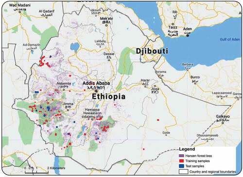
We have selected Ethiopia, a country in East Africa, as the study area for this work (Figure 1). Ethiopia has a diverse climate and geography with yearly rainfall in a range of below 200 mm to over 2400 mm and altitudes ranging from 125 m below sea level to 4533 m above sea level (Friis, Sebsebe, and van Breugel 2010, & reugel, 2010). The rainfall for most parts of the country occurs in two seasons, between March to April and June to September. Ethiopia possesses high forest biodiversity consisting of about 7000 higher plant species. 12% of plant species are endemic to Ethiopia (Berhan and Egziabher 1991). Due to its long history of high deforestation rate caused by increasing population and hence increased clearing for agriculture, grazing, and settlements (Bishaw 2001; FAO 2010; Getahun, Poesen, and Van Rompaey 2017), 64 species are identified as threatened in 2018, and 21 species are identified as endangered in the IUCN Red List (Stévart et al. 2019). Over 50 years ago, Ethiopia had about 40% of the forest. At present, that number is close to 15% (BBC 2019), mostly in the south-west of the country. Efforts have been initiated to preserve these remaining forests because of their richness in plant species, for instance, hosting most of the world’s coffee diversity (Lemenih and Kassa 2014). The country has been praised for its efforts to reduce deforestation through forest restoration and regeneration (BBC 2019; UN-REDD 2017). However, in spite of the said effort, the speed of forest loss is still high (Hansen et al. 2013), specifically deforestation related to small-scale and large-scale cropland expansion (Lemenih and Kassa 2014). This work aims at improving the tool-set for data-driven forest management and policy toward sustainable and actionable conservation of Ethiopian forests.

Figure 1. Map showing the spatial distribution of forest loss locations, training and test data across Ethiopia. The colors represent training and testing samples of one of the train-test split. The gray-lines are the boundaries of the study area, regions, and country.

2.2. Data

Three data sources acquired within Ethiopian boundaries were used in this study: (1) the Hansen forest loss, to identify areas of forest loss; (2) Manually annotated reference data, using very high-resolution imagery, containing 11 land uses following deforestation or follow-up land-use (FLU) classes; and (3) satellite imagery data (Planet-NICFI, Sentinel-2, and Landsat-8).

2.2.1. Forest loss data

We made use of the Hansen forest loss data (Hansen et al. 2013) as an interim step in identifying training labels of land-use following deforestation. Hansen forest loss data is a global forest product that has been extensively used to evaluate forest loss. The data provide useful annual spatial and temporal forest loss information on a global scale for as much as 2000 (Zeng et al. 2018). A total of 300 forest loss locations were randomly sampled using Hansen forest loss in Google Earth Engine (GEE) with a buffer of 5 km. However, five were rejected due to cloud cover. The 5 km spacing or buffer ensured that samples are sufficiently spaced to avoid the risk of spatial autocorrelation. The sampled locations were used as priors to visually create or identify FLU training and validation labels.

2.2.2. Reference data

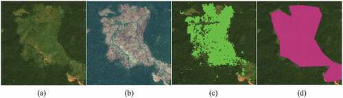
Using seasoned experts and manual interpretation of HRSI from the Planet-NICFI, GEE, and Hansen forest loss data, we visually interpreted the randomly collected reference sample data specifically for classifying FLU in Ethiopia (Figure 1). The task of interpreting and collecting the reference FLU was conducted during July and August 2021. The Hansen-derived forest loss from 2010 to 2014 (Hansen et al. 2013) was used as a baseline for identifying the forest loss areas, while HRSI from the Planet-NICFI for 2016 and GEE was used for identifying and digitizing the FLU as polygons (Figure 2). In addition, other data sources such as the Ethiopia Sentinel-2 Land-Use Land-Cover 2016 map, forest cover change map for year 2000–2013 based on Landsat images and the Ethiopia Mining Cadastre were also helpful to aid in interpreting and digitizing the FLU classes (Ministrry of Mines and Petroleum 2021; RCMRD 2018; UN-REDD 2017). Here, we adopt the definitions of FLU presented in Masolele et al. (2021), corresponding to IPCC main FLU classes (IPCC 2013). The FLU classes were identified in consultation with representative stakeholders from Ethiopia such as the National REDD+ Secretariat, Environment, Forest and Climate Change Commission (EFCCC), Oromia REDD+ Coordination Unit, FAO – Ethiopia, Ethiowetlands, International Center for Tropical Agriculture (CIAT), Ethiopian Geospatial Information Agency, Ethiopian Environment and Forest Research Institute (EEFRI), Farm Africa, and Center for International Forestry Research-World Agroforestry (CIFOR-ICRAF).

Figure 2. Figure For the same location in Ethiopia, (a) Planet-NICFI image, (b) Google earth engine image used for visual interpretation, (c) Hansen forest loss and, (d) manually annotated reference polygon. Example imagery and polygon were retrieved from Google Earth Engine

The collected labels consist of six main land-use classes, namely, Agriculture, Infrastructure, Mining, Water, Tree plantations, and Others. The main land-use classes were further divided into 11 more detailed FLU classes see details as provided by Masolele et al. (2021), i.e. large-scale cropland (20.0%), small-scale cropland (30.2%), pasture or free grazing (6.5%), roads (3.0%), tree plantation (3.5%), coffee crops (10.5%), tea plantation (10.0%), mining (7.0%), buildings and dams (2.3%), other land with tree cover (1.2%), and water (5.8%). In Figure 1, we present the reference data showing the spatial distribution of FLU used in this research. The ground-truth data are polygons relative to the forest loss per FLU in Ethiopia for the 11 selected FLU classes. It is important to note that the tree plantation class is often not related to the loss of natural forest. Tree plantations are often cleared for sustainable forestry management and typically grow back over time between rotational periods. This class was included in this study to avoid confusion with other FLU since the harvested patches from forest plantations are shown in the Hansen data as forest loss.

In total, we annotated 237 tiles used for model training and an additional set of 28 and 30 images as test sets stemming from disjoint locations for the years 2016 and 2020 based on forest loss from 2010 to 2014 and 2015 to 2019, respectively. This was important to evaluate the spatial and temporal robustness of our model Figure 1.

2.2.3. Satellite data

We used Planet-NICFI, Sentinel-2, and Landsat-8 satellite imagery to classify land-use following deforestation. The imageries have a spatial resolution of 4.77 m, 10 m, 30 m, and a maximal temporal resolution of bi-annual, 5, and 16 days, respectively. For this study, we used bi-annual images to match the temporal resolution of Planet-NICFI images. We selected these satellite images to assess the usefulness of different spatial resolutions for characterizing FLU. For Planet-NICFI imagery, we used analysis-ready, PlanetScope Surface Reflectance Mosaics¹ covering a period from December 2015 to May 2016. The Planet-NICFI images are a product of KSAT and Airbus. They are HRSI made open-source (noncommercial) by Planet Lab through NICFI in order to assist protect forest and biodiversity and reduce the impact of climate change (NICFI 2021). The images come with four spectral bands, specifically – Blue, Green, Red, and Near-Infrared NICFI 2021, plus 3-vegetation indices (NDWI – the normalized difference water index, SAVI – the soil-adjusted vegetation index, and NDVI – the normalized difference vegetation index), resulting in seven bands in total.

Median composite images (December 2015 – May 2016) for Sentinel-2, and Landsat-8 images were also collected for each sample location using GEE. The images cloud filtering was performed by use of the quality assessment band of Sentinel-2, and Landsat-8 (Cook et al. 2014). The final image composite was created using images with less than 50% of cloud cover. For each median composite, the NDVI, the SAVI, the normalized buildup index (NDBI), and the normalized difference moisture index (NDMI) were computed. Each composite image for Landsat-8 included seven spectral bands (e.g. Blue, Green, Red, Near-Infrared, Shortwave infrared-1, Thermal-infrared, and shortwave infrared-2) and four vegetation indices (SAVI, NDVI, NDMI, and NDBI), resulting in a total of 11 bands. On the other hand, the composite image for Sentinel-2 consisted of 10 spectral bands (Blue, Green, Red, 3-Vegetation red edge bands (B5, B6, and B7), Near-Infrared, Narrow Near-Infrared, Shortwave infrared-1, and shortwave infrared-2), plus four indices (SAVI, NDVI, NDMI, and NDBI), resulting in a total of 14 bands. All sentinel-2 bands were resampled to 10 m. Overall, the satellite data collected comprise 4, 7, and 10 spectral bands (plus 3, 4, 4 vegetation indices each for Planet-NICFI, Landsat-8, and Sentinel-2, respectively) from 2016.

Additionally, four composite images, each with the same number of bands as the above images, were collected from four different time steps for multi-date image analysis. The composite images were acquired from (December 2015–May 2016, June 2016–November 2016, December 2016–May 2017, and June 2017 – November 2017). The multi-date images were essential to add the temporal dimension in classifying the FLU.

2.2.4. Data preprocessing

Using 295 sampled forest loss location across the country, we manually delineated rectangular polygons around sampled locations to download images (tiles) from GEE for each data source (Planet-NICFI, Sentinel-2, and Landsat-8). From each downloaded image tile, patches of dimensions $x_i\in {\mathbb{R}}^{w\times h\times d}$ and the corresponding FLU labels $y_i\in {\mathbb{R}}^{w\times h\times c}$ were extracted, where $w$, $h$ ,and $d$ specify the width, height, and number of bands of an image patch and $c$ specifies the number of classes. The patch dimensions for each modality were, respectively $128\times 128$, $64\times 64$, $32\times 32$ pixels, to account for the different resolutions. Patches were extracted such that each would have a $3/4$ overlap with others, in an effort to decrease the loss of data used for training due to border effects. Each band $j\in \{1,\dots ,d\}$ of a given image patch $x_i$ was normalized via min-max scaling by resorting to the minimum and maximum pixel value for that band across all the training-images such that the resulting pixel values were in the range from 0 to 1.

2.3. Deep learning models for FLU classification

Two semantic segmentation DL architecture, inspired by U-Net (Ronneberger, Fischer, and Brox 2015), were tested to characterize FLU using Planet-NICFI, Sentinel-2, and Landsat-8 satellite imagery. The U-Net architecture was chosen as a starting point due to its efficiency in extracting features and spatial patterns from satellite data, even in the case of limited training data (Gallwey et al. 2020; F. Zhao et al. 2022). In particular, we consider the following two variants:

1. A standard U-Net architecture, which uses convolution operations to retrieve spatial features from images at different scales of an image. The coarse activation maps highlight contextual-rich information and underscore the type and position of global descriptors. The activation maps retrieved along different scales are subsequently combined via shortcut connections to join coarse and higher-level predictions (Descals et al. 2021b; Irvin et al. 2020; Ronneberger, Fischer, and Brox 2015). Refer to the architecture details in the Appendix A1

2. Attention U-Net, which integrates attention gates into the standard U-Net architecture to accentuate important descriptors that are passed via the shortcut connections. This is important as pieces of information retrieved from lower layers are used in the attention gate layer to amplify unimportant and noisy features in shortcut connections (Oktay et al. 2018; Schlemper et al. 2019). We adapted the design of the attention module to the multi-class setting by learning one attention map per feature map. Without this adaptation, the models in (Oktay et al. 2018; Schlemper et al. 2019), developed to remove the background information in foreground/background segmentation tasks, tend to completely remove information from some of the image areas, negatively affecting performance.

The details for implementation of each model are described in the subsequent section and its summary in Appendix B. The computational consideration is described in Appendix F. The figures of individual model designs are described in Appendix A. We also provide the flowchart showing the workflow of this research in Appendix C.

2.4. Implementation details

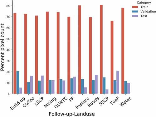
In this section, we talk about hyperparameter optimization and model implementation. We split the training dataset 3-times in a ratio of 90% and 10% for training and validation important for three-fold cross-validation (Figure 3). We use Bayesian optimization to choose the model parameters (see below Appendix B) based on one of the folds see details as provided by Masolele et al. (2021), in which the best model parameters for U-Net and Attention U-Net models are chosen on the basis of accuracy attained on the validation data. The ultimate model architecture was then evaluated on the held-out test data for each run. Thus, in this paper, we report the mean and standard deviations of the accuracies on the test data over the threefolds (Masolele et al. 2021). We describe the final allocation of the best parameters in Appendix B.

Figure 3. The training, validation, and test data showing the number of pixels per FLU (in %) of one of the random splits. Where SSCP, OLWTC, PF, LSCP, and TeaP correspond to small-scale cropland, Other land with tree cover, tree plantation, large-scale cropland, and tea plantation, respectively

Both models were created using the Keras library (Chollet 2015) and TensorFlow (Abadi et al. 2015) as backend. All models were trained for 100 epochs using a batch size of 64. For every convolutional layer, we added a padding operation to ensure that the size of the last layer stays comparable to the input layer and followed by a non-linearity function-ReLU (Appendix B1). The features in the convolution layers were normalized using Batch normalization followed by a regularization dropout rate of 0.1. All models were optimized by using Adam optimizer with a learning rate (lr) of ${10}^{-3}$ . The optimized loss was a sum of multi-class categorical Focal Loss and Dice Loss of the post-softmax probability and the one-hot label analogous to the land-use class of the pixels of the image patch. Every one of the associated tasks was performed using Python in the Sepal geospatial analysis platform FAO (2021).

2.4.1. U-Net

This is a direct adaptation of the standard U-Net architecture (Ronneberger, Fischer, and Brox 2015) that receives images from a single time step of shape (width × height × bands), along with the corresponding label maps. The model architecture is made up of an encoding followed by a decoding section. For the encoder, we have used four successive convolution layers with 3 × 3 filters, each followed by a pooling layer, resulting in a set of 512 feature maps. The encoder section is designed such that at each block the number of feature maps is increased by a factor of 2, while its spatial size is decreased by a factor 2. This is useful to increase the receptive field during the convolution operation. It also allows the model to increasingly retrieve semantic-contextual information. The decoder is the reverse of the encoder, by which the convolution layer is followed by upsampling layers instead of the pooling layers. The output maps of the decoders have the same spatial dimensions as the input data. The coarse and fine feature maps extracted at various blocks of the encoder and decoder section are combined through shortcut connections as shown in (Appendix A1). Finally, the softmax activation functions were used to obtain the final segmentation results.

2.4.2. Attention U-Net

As an improvement to the standard U-Net, we incorporated attention gates, in a fashion similar to those proposed by Oktay et al. (2018), into the standard U-Net architecture to accentuate predominant descriptors that are passed via the shortcut connections (see Appendix A2). Unlike in Oktay et al. (2018), we compute one attention map per feature, instead of all features sharing the same attention map in each attention gate, in order to adapt the method to the multi-class setting. In this way, the attention gates learn features passed through the skip connections to model location and relationship between FLU at local scale, thus improving the detection of small-scale and complex FLU, i.e. roads, settlement, small-scale cropland. This is important as pieces of information retrieved from lower layers are used in the attention gate layer to amplify unimportant and noisy features in shortcut connections. The gating operation is done prior to the concatenation step to combine only important activations. In addition, in both forward-and backward pass, the neuron activations are filtered (Schlemper et al. 2019). This enables the parameters in the lower layers to be updated largely in the context of spatial locations that are important to a specific class Oktay et al. (2018).

2.4.3. Ensemble of Attention U-Nets

Finally, we consider an ensemble of different models trained on single-date Planet-NICFI, Sentinel-2, and Landsat-8 data, respectively. The ensemble is based on the late fusion of probability maps of the output of the three Attention U-Net models from single-date Planet-NICFI, Sentinel-2, and Landsat-8. Since the satellite data and, hence, the prediction maps are available in different spatial resolutions (there are three resolutions in our scenario; “Planet-NICFI model,” “Sentinel-2 model,” and “Landsat-8 model,” equivalent to image patches with a resolution of 4.77 m, 10 m, and 30 m, respectively), we first upscale the prediction maps that stem from the Sentinel-2 and Landsat-8 data to match the resolution of the Planet-NICFI model (via nearest neighbor upscaling). The output of the ensemble is then based on the average probabilities induced by these three Attention U-Net models, where the final prediction per pixel is the class with the highest mean value.

2.5. Evaluation of models

Typically, land-use classification and related tasks are evaluated based on spatially sampled data acquired at the same time step. For this study, however, the same model is validated two times on spatial and temporal test datasets to predict the FLU for other years. Thus, we evaluated the performance of our DL models in identifying the FLU (1) by use of held-out test data for 2016 (the same year as training data) and applying a threefold approach, and (2) using the test dataset of FLU for 2020 (Section. 3.4). For each model, we used Precision $P=TP/(TP+TN)$, Recall $R=TP/(TP+FN)$, F1-scores $F1=2\cdot P/(P+R)$, micro-and macro average of F1-scores as the evaluation metrics, where $TP$, $TN$, and $FN$ stand for true positives, true negatives, and false negatives, respectively. More details can be seen in (Masolele et al. 2021).

2.6. Wall-to-wall prediction

Once the best-performing satellite imagery and DL model were identified using the F1-score (Section 2.5), we then used this satellite imagery and model to predict land-use following deforestation in Ethiopia for the study period of 2016 using the areas known to be covered by tropical forest in 2010 (FAO 2010) and forest loss data in 2010–2014 as a mask (Hansen et al. 2013).

After land-use was classified, we estimated the proportions of each of land-use following deforestation per loss area based on Ethiopian regions (Abebe et al. 2019; FAO 2010) and forest type (Dinerstein et al. 2017). This is important to show the patterns and dominance of different deforestation drivers for each regions and forest type for better conservation actions and data-driven land-use policy decisions.

2.7. Accuracy assessment of the wall-to-wall product

To evaluate the accuracy of the final wall-to-wall land-use product, we conducted independent assessments based on the visual interpretation of bi-annual Planet images. We used stratified estimation of area, and accuracy Olofsson et al. (2014) to estimate the number of samples required to assess the output map of direct drivers of forest loss. First, the area of each land-use class was estimated from the map product, followed by calculating the proportion of each class of drivers of forest loss. For each class, sample estimation weights were calculated. The resulting weights were used to calculate the number of samples required to assess the accuracy of the map for each land-use class. In total, 770 samples were collected and interpreted (Figure E1). Following these, the accuracy of the map was calculated using the F1-score, user’s and producer’s accuracies.

3. Results

We start by presenting the results of the classification of FLU for single-date, multi-date, and an ensemble of Planet-NICFI, Sentinel-2, and Landsat-8 images using a deep learning model (namely Attention U-Net), for identifying the FLU in Ethiopia. In Section 3.1 we present the FLU classification results comparing the performance of U-Net and Attention U-Net models. We then explore the classification results of FLU based on single-date Planet-NICFI, Sentinel-2, and Landsat-8 data using the Attention U-Net model (Section 3.2). In Section 3.3, we report the performance of FLU classifications from single-date image prediction, multi-date image prediction, and ensemble of multi-sensor image prediction, using test data from the same year as training data (2016). In Section 3.4, we compare the accuracy score of FLU prediction using forest loss test data from year 2016 and year 2020. Eventually, in section 3.6, we show the spatial pattern and proportions (%) of land-use following deforestation per region and forest type in Ethiopia.

3.1. Model comparison

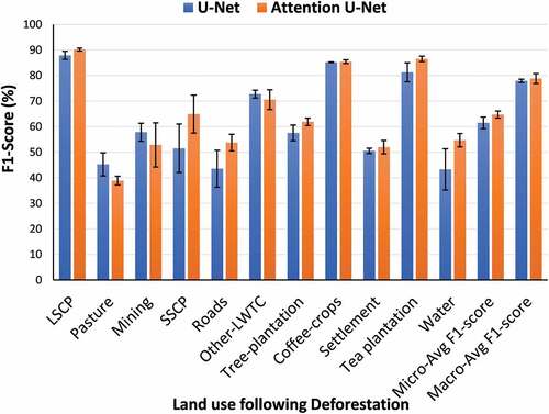
In this section, we highlight the advantage of adding the attention mechanisms to the standard U-Net model using Planet-NICFI data. The Attention U-Net model achieved relatively higher accuracy than the standard U-Net model (Figure 4). For most FLU classes, both models obtain near similar levels of accuracy except for FLUs with smaller footprints such as small-scale agriculture, settlement, and roads where the standard U-Net tends to lag behind the Attention U-Net by a large margin (Figure 4) .

Figure 4. The classification F1-scores of FLU using standard U-Net, and Attention U-Net models in Ethiopia. SSCP and LSCP correspond to small-scale cropland and large-scale cropland, while Other-LWTC correspond to other land with tree cover. For each F1-score, we show the standard deviation represented as error bars.

3.2. Performance of single-date Planet-NICFI, Sentinel-2, and Landsat-8 satellite imagery

The FLU classification model based on single-date Planet-NICFI data outperformed the models based on single-date Sentinel-2, and Landsat-8 data, as shown in Figure 5. The Planet-NICFI model attained a macro- and micro-average F1-score of 79%, 65% compared to 70%, 59% for Sentinel-2, and 70% and 54% for Landsat-8 model.

Figure 5. The classification F1-scores of FLU using Attention U-Net models in Ethiopia. The F1-scores are based on single-date, multi-date, and an ensemble of image predictions for Planet-NICFI, Sentinel-2 and Landsat-8 data. SSCP and LSCP correspond to small-scale cropland and large-scale cropland, while Other-LWTC correspond to other land with tree cover. The error bars are the standard deviation on F1-scores

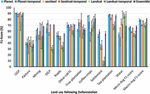
The higher score by planet-NICFI model is particularly observed for the FLU type, large-scale cropland (90%), mining (53%), small-scale cropland (72%), roads (54%), coffee crops (86%), settlement (52%), and tea plantation (85%). The exception is water, where Sentinel-2 and Landsat-8 based models outperformed Planet-NICFI based model, possibly due to additional spectral bands in the short-wave region of the spectrum useful for monitoring water variability (Figure 5). On the other hand, pasture and small-scale cropland are likely to be incorrectly predicted as other land with tree cover by (27%, 12%), respectively. Settlements and tree plantations are often misclassified as other land with tree cover, 31% and 43% of the test samples, respectively (Figure D4). This results are based on image acquired on a single time-step.

3.3. Performance of single-date image predictions, multi-date image predictions, and ensemble prediction

As we expected, the F1-classification scores were higher for the single-date planet-NICFI, ensemble, and multi-date medium resolution image predictions compared to the single-date medium resolution image predictions (Figure 5).

Interestingly, the increase in F1-score when moving to multi-date imagery is only consistent in the case of Sentinel-2 imagery, where it improves for all classes and for the overall FI-scores. For example, prediction accuracies increased for large-scale croplands (from 87% to 90%), coffee crops (from 51% to 66%), mining (from 50% to 52%), roads (from 48% to 50%), and tea Plantation (from 81% to 87%). Also, higher micro (59% to 66%) and macro (70% to 77%) average F1-scores were obtained. In the case of Landsat-8, improvement in F1-score is observed mostly for large-scale land-uses such as large-scale cropland (from 77% to 86%), tree-plantation (from 58% to 63%), coffee-crops (from 71% to 75%), and tea-plantation (from 67% to 70%). For planet-NICFI improvement in F1-score is observed for small-scale land-uses such as mining (from 53% to 64%), small-scale croplands (from 65% to 74%) and settlement (from 52% to 60%) (Figure 5).

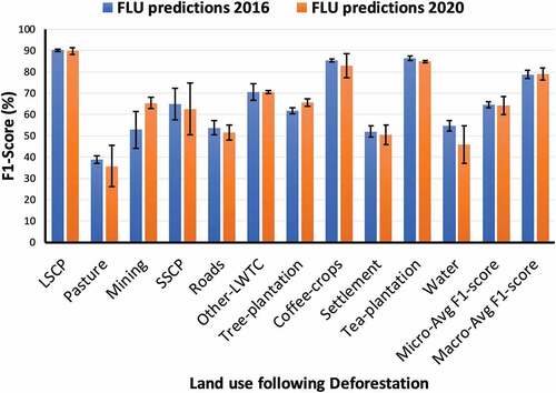
3.4. Temporal robustness

We further analyzed the robustness of our approach over independent data (Planet-NICFI) from different time steps (2020), based on forest loss from 2015 to 2019. The earlier FLU predictions using Planet-NICFI images of 2016 (Figure 5) are based on forest loss from 2010 to 2014. The 2016 FLU prediction results are compared with FLU prediction results from 2020 test data. This step is necessary to investigate the capability of our approach in generalizing across spatial locations and time. As indicated in Figure 6, relatively similar micro- and macro-average F1-scores (65%, 64% and 79%, 79%) were obtained when predictions are made for year 2016 and 2020.

Figure 6. The classification F1-scores of FLU using for planet-NICFI images acquired in year 2016 and 2020. SSCP and LSCP correspond to small-scale cropland and large-scale cropland, while Other-LWTC correspond to other land with tree cover. The error bars are the standard deviation on F1-scores

3.5. Wall-to-wall product

The accuracy assessment of wall-to-wall map using stratified estimation of area and accuracy using planet-NICFI showed the reliability of the final land-use following deforestation product produced by the Attention U-Net model. The most validated FLU had an accuracy higher than 0.8% (Table 1), with the exception of mining (0.73%). These accuracy results are consistent with the model performance accuracies obtained in Section 3.3, which further proves the robustness of our proposed method for mapping land-use following deforestation.

Table 1. Accuracy metrics of the wall-to-wall map from independently sampled validation data. SSCP and LSCP correspond to small-scale and large-scale cropland and PF for plantation forests. All the accuracies are reported as average values and 95% confidence intervals for each class.

FLU	User’s accuracy (%)	Producer’s accuracy (%)	F1 (%)
LSCP	$95\pm 3.6$	$92\pm 4.5$	$94\pm 3.9$
Pasture	$84\pm 10.2$	$88\pm 9.0$	$86\pm 9.6$
Mining	$100\pm 0.0$	$57\pm 13.7$	$73\pm 12.3$
SSCP	$90\pm 8.3$	$94\pm 6.5$	$92\pm 7.5$
Roads	$96\pm 5.4$	$100\pm 0.0$	$98\pm 3.8$
PF	$86\pm 9.6$	$88\pm 9.0$	$87\pm 9.3$
Coffee	$97\pm 4.7$	$92\pm 7.5$	$94\pm 6.6$
Settlement	$94\pm 6.6$	$96\pm 5.4$	$95\pm 6.1$
Tea	$96\pm 5.4$	$100\pm 0.0$	$98\pm 3.9$
Water	$100\pm 0.0$	$80\pm 11.1$	$\hspace{0.17em}88\pm 9.0$

3.6. Regional patterns of land-use following deforestation

Using the HRSI and Attention U-Net, we classify and map the FLU per forest loss location in Ethiopia based in regions and forest types where forest loss occurs. The map in Figure 7 shows forest being heavily cleared for the establishment of small-scale croplands in regions like SNNPR² Oromia, Gambela, and Benishangul Gumuz (Figure 8a). Small tracts of forest have also been cleared for small-scale croplands in Amhara region. Bright hotspots of forest loss for coffee crops are most prevalent in the northwest and east of SNNPR and Gambela regions, respectively, while large-scale croplands are most prevalent in Gambela, Benishangul Gumuz, SNNPR, and Oromia regions, respectively. Nevertheless, we can also see a confusion between small-scale cropland with pasture and other land with tree cover, particularly in Gambela and Benishangul Gumuz. Another confusion can be seen in SNNPR between other land with tree cover and coffee crops (mainly in the district of Guraferda) Figure D1. In (Figure 7), we show detail maps (zoomed in) of some of the areas indicated by B, C, D, E, F, and G. Detail maps show the local patterns exhibited by each type of land-use following deforestation including (B) Coffee crops (teal), (C) Small-scale cropland (orange) and settlement (pink), (D) roads (red), settlement (pink), and dam construction in the woodlands of Benishangul Gumuz, (E) Large-scale croplands (yellow), (F) small-scale croplands, and (G) Tea plantations (cyan). New roads (red), as detected in (D), (E), (F), and (G), provide accessibility to patches of land-use.

Figure 7. Classified land-use post-deforestation for the Ethiopia tropical forest for the period 2010 through to 2014. The green in A is NDVI base map showing areas with forest cover as retrieved from USDA (2017). Areas indicated by b, c, d, e, f, and g are shown in zoomed in maps. Zoomed in maps show local patterns of the follow-up land-use with planet-NICFI as a base map. (b) Coffee crops (teal), (c) Small-scale cropland (orange) and settlement (pink), (d) Roads (red), settlement and dam construction (pink) in the woodlands of Benishangul Gumuz, (e) Large-scale croplands (yellow), (f) small-scale croplands (orange), and (g) Tea plantations (cyan). New roads (red) as detected in (d), (e), (f), and (g) provides accessibility to patches of land-use. SSCP, LSCP, PF correspond to small-scale cropland, large-scale cropland, and tree plantation while OLWTC correspond to other land with tree cover

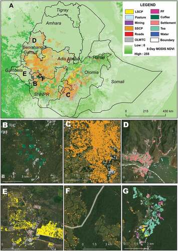
Figure 8. Proportions of post-deforestation land-use, (a) per region, and, (b) per forest type, for the Ethiopia tropical forest for the period 2010 through to 2014. SSCP correspond to small-scale cropland, LSCP to large-scale cropland, EMF to Ethiopia montane forests, MGS to montane grasslands and shrublands, TSGSS to tropical subtropical grasslands-savanna and shrublands, and DXS to Deserts and Xeric shrublands.

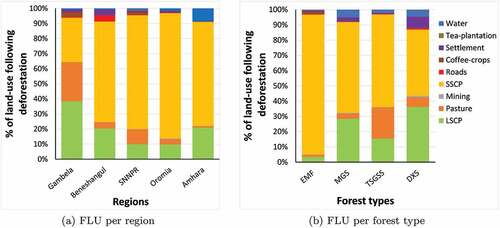
Likewise, the results of FLU prediction based on forest types (Figure 8b) follow similar spatial patterns to predictions based on regions (Figure D1, Figure 7). Small-scale cropland is the dominant FLU observed in all Ethiopian forest types.

Croplands (SSCP, LSCP, coffee, and tea plantations) dominate the FLU in all of the regions and all of the forest types (73%, 15%, 0.75%, 0.21%), with the majority of small-scale croplands establishments being observed in the Ethiopian montane forests, especially on forest edges, while large-scale croplands are observed in montane grasslands and shrublands, deserts, and xeric shrublands, as well as tropical and subtropical grasslands, savannas, and shrublands (Figure 8b).

4. Discussion

Our results confirm the usability of U-Net Ronneberger, Fischer, and Brox (2015) style CNN architectures for large scale FLU mapping using either Landsat-8, Sentinel-2, or Planet-NICFI imagery. They also show that it is advantageous to use a multi-class version of Attention U-Net Oktay et al. (2018).

As expected, we observed a strong correlation between spatial resolution and FLU classification performance, with Planet-NICFI imagery resulting in the best overall results even if it provides less spectral resolution than the other sources (Section. 3.2). This confirms that more detailed spatial features are vital to differentiate the FLUs, especially the FLUs with smaller footprints such as settlement, roads, and small-scale cropland. Visually, this is also true as small features are easily identifiable with high-resolution images at local level, as opposed to coarser resolutions, possibly due to mix of different land-use practices at a coarser spatial scale, i.e. new roads passing through forest or new village settlements.

Additionally, we also observed that the use of multi-date data for medium resolution images allows to close the accuracy gap with high-resolution imagery, at least for Sentinel-2 data (Figure 5). This shows that for medium-resolution images, temporal patterns of land-use can compensate from the loss of spatial information stemming from the coarser spatial resolution with respect to the Planet-NICFI imagery, particularly when the problem includes small-scale agriculture and coffee crops. On the other hand, this might suggest a higher level of the temporal variability that distinguishes every land-use, probably because of variation in seasonality and land-use practices in Ethiopia (Masolele et al. 2021).

The performance of all models using the three datasets in identifying pasture versus other FLU classes is relatively low, indicating that pasture is indeed often mixed with other FLU, i.e. small-scale croplands, settlement, and other land with tree cover. This is due to the fact that small holder farmers in Ethiopia keep their livestock close to home and bring them food and water to preserve the newly acquired deforested areas for farming and housing (Dow Goldman et al. 2020). On the other hand, pasture is a rare class, indicating that even greater amount of training data or even temporal data across the same seasons for pasture would be required to cover the spatial heterogeneity of pasture in Ethiopia.

In Section 3.6, we observed that the class other land with tree cover, which includes forest regrowth, is over-predicted in most regions (Figure D1). This is because, although forest loss was detected, the transition to land-use classes such as agriculture, coffee, tea is a slow process and takes time. Looking at the satellite imagery (Figure D2), we see that the forest is cut down in several steps, where parts of the forest are deforested at different points in space and time. Since we use a single deforestation map for the whole period, this can lead to ambiguities in which the model may confuse forest regrowth with yet-to-be cut down forest. A potential solution for next research would be to start looking at what would be the best lag time to detect land-use after deforestation. Our assumption is that the model would perform better in an older deforested area as land-use is more distinct after a few years of human activities (Figure D2). It is also important to note that not all detected forest changes, i.e. in Hansen et al. (2013), were due to land-use conversion, as some of it may also be detected as a result of fire, landslides, and floods, which were not considered in this study.

Small-scale croplands are the dominant cause of forest loss in all regions and forest types of Ethiopia, Figure 8a, Figure 8b and Figure D1. Most of the small-scale clearing occurs at the edge of the forest, as seen in Figure D3. This is the common practice, as deforestation is done by small-scale farmers, often families, who farm a mixture of food, fruit crops, and livestock herds for some years, and when the soil loses its fertility, they let the farms go fallow (Dow Goldman et al. 2020). Forest conversion into large-scale cropland is the second main driver of forest loss. The LSCP typically involves large-scale clear-cutting and is grown on an industrial scale (Figure D1, Figure 7). Most LSCP hotspots can be seen in Gambela, Benishangul Gumuz, and SNNPR regions and in all forest types with the exception of Flooded Grasslands & Savannas, indicating that LSCP is not limited to a single forest type or region (FAO 2010).

In addition to small- and large-scale cropland, the third and fourth dominant drivers of forest loss are pasture and settlement, respectively (Figure 8a and Figure 8b). This observation is in line with the results of recent similar studies (Betru et al. 2019; Hishe et al. 2021; Mengist, Soromessa, and Feyisa 2021; Sisay et al. 2021; Yahya et al. 2020) which used Landsat satellite imagery and focus group discussion to assess proximate drivers of forest loss in different parts of Ethiopia. However, these studies were conducted on few isolated study areas (local scale) and do not provide detailed identification of drivers of forest loss (fewer classes). Our research goes beyond small-scale, pixel-based methods, coarse spatial resolution benchmarking tasks to national scale, deep learning method, and higher spatial resolution images. The increased spatial resolution of the satellite dataset (Planet-NICFI) to 5 m allows for more accurate and detailed identification of small features and those with fine spatial textures such as roads, mining, coffee crops, and village settlement, which would otherwise not be included (NICFI 2021).

Our study contributes to reducing methodological, data, and knowledge gaps in more direct measures of proximate drivers of deforestation in Ethiopia based on satellite image assessments by using a robust semantic segmentation deep learning method. For small-scale and large-scale cropland, pasture, settlements, coffee-crops, roads, and mining, all of which are identified in dramatic forest declines in Ethiopia (Betru et al. 2019; FAO 2010), our method provides a way of mapping the extent of these drivers on forest resources at a national scale. Even for drivers for which satellite imagery maps of land-use conversion exist (for example, agriculture and forest loss), our results provide additional information by offering higher thematic detail. Regional and global analyses (Curtis et al. 2018) have also incorporated information about spatial distributions of land-use to account for where drivers are likely to affect most forests. However, while important, such analyses still assume that drivers of deforestation are uniformly likely across the national scale. Our results show that patterns of deforestation drivers often differ at national scale based on region and forest type. This disparity in part relates to traditional representations of mainly dominant land-use leaving-out some types of land-uses (for instance, “roads” providing accessibility to forests or dams, i.e. in Benishangul Gumuz (Figure D1), “Mining” established deep within forests, “new settlements,” and/or lack of distinction between small and large-scale cropland) (Curtis et al. 2018; FAO 2010; Mengist, Soromessa, and Feyisa 2021). In addition, the effect of these drivers varies with the specific spatial context, so the same intensity of forest loss can have different impacts in different regions or on different forest types (Betru et al. 2019; FAO 2010; Hishe et al. 2021; Mengist, Soromessa, and Feyisa 2021; Sisay et al. 2021; Yahya et al. 2020). For example, small-scale croplands affect a larger proportion of forests in Amhara and Benishangul Gumuz, where a bit of primary forest is left, than in the Gambela, SNNPR, and Oromia where considerable forest remains despite high rates of forest loss in both regions (Hansen et al. 2013). The opposite is true for large-scale croplands. This in turn may also affect the choice of policy process (reforestation or more conservation) to be implemented in either regions.

In summary, although Planet-NICFI or multi-temporal Sentinel-2 data obtained a substantially higher F1-score in identifying most of the FLU classes compared to single-time Sentinel-2 and Landsat-8, the latter can still be seen as an alternative when focusing on certain land-use classes. This is especially true in identifying large-scale land-uses such as large-scale cropland where Planet-NICFI images had relatively similar accuracy as Sentinel-2 and Landsat-8 imagery (Figure 5). Thus, the latter are suitable in regions where large-scale land uses are a dominant cause of deforestation as it does not require intensive computational resource for analysis (Table F1). However, in regions where small-scale land-uses (i.e. Mining, small-scale cropland, and settlements) are a threat to deforestation Planet-NICFI would be the best choice for achieving higher classification accuracies (Figure 5). However, it is important to keep in mind that the use of Planet-NICFI for this type of analysis requires more computational resources (Table F1). Here, the use of open-source cloud-based computational platform like SEPAL (FAO 2021) offers an opportunity to overcome this problem. Ethiopia is piloting the use of Planet-NICFI using SEPAL, which shows that such computational resources are accessible for developing countries like Ethiopia given the right mix of training and tools, opening new paths for the monitoring of the proximate drivers of deforestation at country and, eventually, continental scale.

5. Conclusion

This paper presents the use of high and medium resolution open-access satellite imagery for identifying post-deforestation land-use on a country-level using an Attention U-Net deep learning segmentation method. The land-use classification strategy was applied to a single-date, multi-date and an ensemble of Planet-NICFI, Sentinel-2, and Landsat-8 satellite data. This process relies on the use of a forest loss dataset to select forest loss areas, followed by the creation of a reference dataset through the visual interpretation of land-use following deforestation using Planet-NICFI imagery. Experimental results show that the performance of identifying and mapping land-use following deforestation requires either (1) the use of high-resolution satellite imagery or (2) use of temporal data for medium resolution satellite imagery. We also observed that the addition of an attention mechanism to the standard U-Net segmentation model increases model performance.

Our approach can support a more detailed spatial and temporal analysis of forest loss locations and their proximate drivers. The main contribution of our method is that it presents a new opportunity and possibility to identify land-use. The model can help identify and inform how forest in Ethiopia is currently being affected by a wider range of land-use activities than is currently thought. They can also help report previous and future proximate driver assessments by providing a more systematic and updated understanding of potential driver hotspots over the local and national scales.

Thus, the value of this paper is in illuminating spatial patterns of deforestation drivers and elucidating an approach to identifying causes as well as aid in decision-making within the context of national policy processes, recognizing that understanding the location of different proximate drivers of forest loss is vital for setting up effective forest conservation policy and responses.

In future research, we intend (1) to start looking at what would be the best time to detect land-use after deforestation, (2) to quantify the trend of predominant drivers of forest loss over national and/or continental scale applied for previous and more recent time periods while leveraging seasonality, the availability of dense time series of HRSI and the free and open-source global forest loss data Hansen et al. (2013); Reiche et al. (2021) through Attention U-Net deep learning method.

Data availability

This study was supported by freely and open-source satellite data available from the Google Earth engine at https://code.earthengine.google.com/. Planet-NICFI data can be accessed via https://www.planet.com/pulse/nicfi-tropical-forest-basemaps-now-available-in-google-earth-engine/.

Author contribution

Robert N. Masolele: Creation of the initial concept of this study, development of method, analysis, writing, editing the original draft and article. Veronique De Sy: Creation of initial concept of this study, article review, and editing. Diego Marcos: Development of methods, writing and editing of the article and article review. Jan Verbesselt: Creation of the initial concept of this study and editing of the article. Fabian Gieseke: Methodology and editing – article. Kalkidan Ayele Mulatu: Conceptualization of reference data and collection. Yitebitu Moges: Conceptualization of reference data and collection. Heiru Sebrala: editing – article. Christopher Martius: Conceptualization of this study and editing – article. Martin Herold: Creation of initial concept of this study, methodology, editing – article.

Acknowledgements

We thank SEPAL – a big-data platform for retrieving and processing remote-sensing data for land monitoring of the Food and Agriculture Organization of the United Nations (FAO) – for providing access to its cloud computing platform. We also thank the Ethiopian Forest stakeholders for their participation and input in this study.

Disclosure statement

We declare that there are no known competing financial interests or personal relationships that could have appeared to influence the work reported in this paper.

Additional information

Funding

This research was carried out as part of CIFOR’s Global Comparative Study on REDD+ (www.cifor.org/gcs). The research is mainly funded by the International Climate Initiative (IKI) of the German Federal Ministry for the Environment, Nature Conservation, Building, and Nuclear Safety (BMUB) 20_III_108. The other funding partners that have supported this research include the Norwegian Agency for Development Cooperation (Norad) 1500551, and the CGIAR Research Program on Forests, Trees, and Agroforestry (CRP-FTA) with financial support from the CGIAR Fund Donors. This research is also funded by the European Commission Horizon Europe project “Open-Earth- Monitor” (Grant number 101059548), the CGIAR initiative MITIGATE+.

Notes

1 planet_medres_normalized_analytic_2015-12_2016-05_mosaic.

2 Since 2020 SNNPR has “split off” into two regions, Sidama & South West Ethiopia Peoples’ regions. Here we are referring to the region before the split.

6. Appendices

Appendix A. Diagrams of individual deep learning model architectures

Figure A1. Schematic view of our U-net network for single-date images input. Inputs are tensors are of size i width $\times$ j height $\times$ n bands. The colors represents, white = Input array, teal = Double 2D convolution operations, and cyan = output layer.

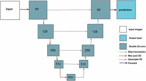
Figure A2. Schematic view of our Attention U-net network for single-date images input. Inputs are tensors are of size i width $\times$ j height $\times$ n bands. The colors represents, white = Input array, teal = Double 2D convolution operations, red = Attention gate, and cyan = output layer.

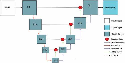
Figure A3. Schematic view of our Attention U-net network for multi-date images input. Inputs are tensors from four time steps (time 1 to time 4), each of size t time steps $\times$ i width $\times$ j height $\times$ n bands. The model operates on a sequence of four input tensors, each composed of n bands. The network architecture automatically detect the useful features of the multiple input bands and combines this information for the following layers to predict the Land-use following deforestation. Note that this model setting is also useful to handle scenarios where either one of the input images are affected by clouds.

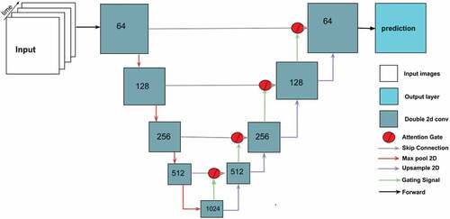
Appendix B.

model parameters

Table B1. Architecture of a standard U-Net, Attention U-Net, temporal Attention U-Net, and ensemble of multi-sensor Attention U-Net models

Parameters	Model type and dimensions
	Standard U-Net	Attention U-Net	Temporal Attention U-Net	Ensemble
Input shape Planet-NICFI	128 × 128 × 7	128 × 128 × 7	128 × 128 × 28	128 × 128 × 28
Input shape Sentinel-2	64 × 64 × 12	64 × 64 × 12	64 × 64 × 48	64 × 64 × 48
Input shape Landsat-8	32 × 32 × 12	32 × 32 × 12	32 × 32 × 48	32 × 32 × 48
No. conv layers	20	20	20	20
No. filter encoder	32, 64, 128, 256, 512, 1024	32, 64, 128, 256, 512, 1024	32, 64, 128, 256, 512, 1024	32, 64, 128, 256, 512, 1024
No. filter decoder	32, 64, 128, 256, 512, 1024	32, 64, 128, 256, 512, 1024	32, 64, 128, 256, 512, 1024	32, 64, 128, 256, 512, 1024
Filter size	3 × 3	3 × 3	3 × 3	3 × 3
Padding	Same	Same	Same	Same
Pool size	2 × 2	2 × 2	2 × 2	2 × 2
Strides	1 × 1	1 × 1	1 × 1	1 × 1
Attention gate	–	Yes	Yes	Yes
Learning rate	0.0001	0.0001	0.0001	0.0001
No. of classes	11	11	11	11

Appendix C.

Workflow of this study

Figure C1. The flowchart showing the steps in data generation, modeling, map validation in our study.

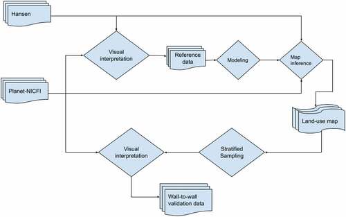
Appendix D.

Spatial patterns of land-use following deforestation

Figure D1. Spatial pattern of classified land-use following deforestation for the Ethiopia tropical forest for the period 2010 through to 2014. The map shows the follow-up land-use predicted using planet-NICFI image. Street map is used as a base map for display. SSCP and LSCP correspond to small-scale cropland and large-scale cropland, PF to tree plantation, and OLWTC to other land with tree cover.

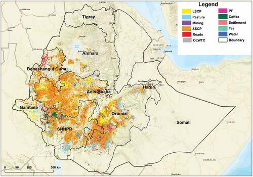
Figure D2. Represents the planet-NICFI images, showing how FLU evolves over time from deforestation. This is one of the patches of land-use following deforestation (large-scale cropland) in Ethiopia where changes happened over n-years, (a) Planet-NICFI image 2016, (b) Planet-NICFI image 2017, (c) Planet-NICFI image 2018 and, (d) the Planet-NICFI image 2020, respectively.

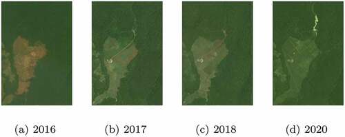
Figure D3. Classified land-use following deforestation for the Ethiopian tropical forest for the period 2010 through to 2014. Areas in orange color are the predicted small-scale clearing occurring at the edges of the forest. Roads in red color provides accessibility on new established patches of land-use following deforestation. SSCP and LSCP correspond to small-scale cropland and large-scale cropland, PF to tree plantation, and OLWTC to other land with tree cover.

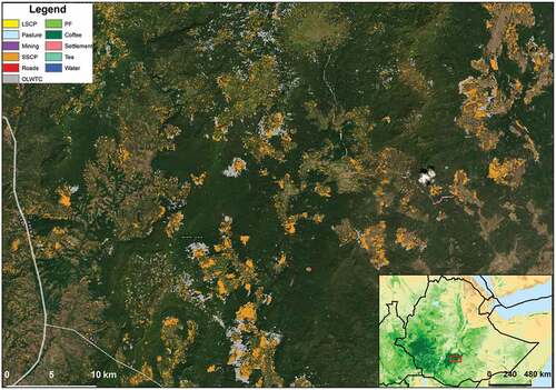
Figure D4. The percentage of true- and false predicted FLU’s using Attention U-Net deep learning method and Planet-NICFI images. SSCP and LSCP correspond to small-scale cropland and large-scale cropland, TP to tree plantation, TeaP to tea plantation, and OLWTC to other land with tree cover.

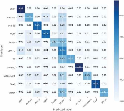
Appendix E.

Wall-to-wall validation samples

Figure E1. Visually interpreted data used for wall-to-wall validation of the land-use following deforestation product. SSCP and LSCP correspond to small-scale cropland and large-scale cropland, and OLWTC to other land with tree cover.

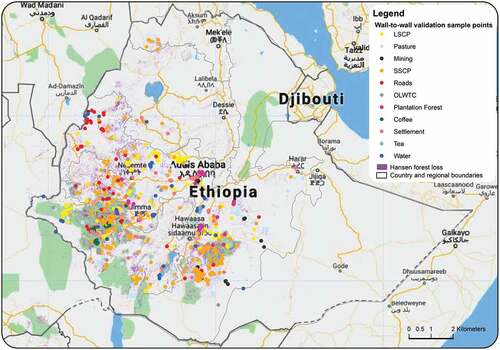
Appendix F.

Computational Considerations

The use of high-resolution Planet-NICFI and ensemble of multi-sensor data was more computationally expensive during training versus using the Sentinel-2 and Landsat-8 data (Table F1). This is due to the high number of pixels per unit in planet-NICFI data compared to Sentinel-2 and Landsat-8 data resulting in increasing computational resource and time demand. Likewise, ensemble model requires training multiple models to retrieve predictions, hence requiring more time on data preparations for training, testing, and when making predictions. Likewise, in testing time, we also observed slight differences between the datasets. This is useful information in relation to resource availability. The choice of whether to use high-resolution images or ensemble or high temporal medium resolution images will depend on available computational resources and time.

All data preprocessing, analysis, and model development were done in (SEPAL 2.0). A cloud-based computing environment of FAO with instance type g8, NVIDIA Tesla M60 GPU 32GB RAM.

Table F1. The time for training and testing in minutes (m) of attention deep learning models using Planet-NICFI, Sentinel-2, and Landsat-8 datasets over a single-date, multi-date, and ensemble approach.

Model	Planet-NICFI		Sentinel-2		Landsat-8		Ensemble (Planet-NICFI, Sentinel-2, Landsat-8)
	Training (m)	Testing (m)	Training (m)	Testing (m)	Training (m)	Testing (m)	Training (m)	Testing (m)
Single-date	1880.47	3.96	212.58	2.45	115.39	1.55	2208.4	6.96
Multi-date	4300.02	5.52	621.55	3.56	219.14	2.212	5140.71	8.63

References

- Abadi, M., P. Barham, J. Chen, Z. Chen, A. Davis, J. Dean, and X. Zheng (2015), 5. “TensorFlow: A System for Large-scale Machine Learning. In Proceedings of the 12th Usenix Symposium on Operating Systems Design and” implementation, osdi 2016, Savannah (pp. 265–283). USENIX Association. Retrieved from https://www.tensorflow.org/
- Abebe, S. T., A. B. Dagnew, V. G. Zeleke, G. Z. Eshetu, and G. T. Cirella. 2019. 4. “Willingness to Pay for Watershed Management”. Resources 8 2: 77. Retrieved from https://www.mdpi.com/2079-9276/8/2/77/htmhttps://www.mdpi.com/2079-9276/8/2/77
- BBC. (2019), 12. Did Ethiopia Plant Four Billion Trees This Year? - BBC News. Retrieved from https://www.bbc.com/news/world-africa-50813726
- Berhan, T., and G. Egziabher. 1991. 12. “Diversity of the Ethiopian Flora”. Plant Genetic Resources of Ethiopia 75–81. Retrieved from https://www.cambridge.org/core/books/plant-genetic-resources-of-ethiopia/diversity-of-the-ethiopian-flora/9E151D8976760F516711EFDB21AAF4B8
- Betru, T., M. Tolera, K. Sahle, and H. Kassa. 2019. “Trends and Drivers of Land Use/Land Cover Change in Western Ethiopia.” Applied Geography 104 (104): 83–93. doi:10.1016/j.apgeog.2019.02.007.
- BioCarbon Fund. (2020). “BioCarbon Fund Initiative for Sustainable Forest Landscapes” (Tech. Rep.). Retrieved from https://biocarbonfund-isfl.org/ISFL-2020-Annual-Report/index.html#intro
- Bishaw, B. 2001. “Deforestation and Land Degradation in the Ethiopian Highlands: A Strategy for Physical Recovery”. Northeast African Studies 8 (1): 7–25. Retrieved fromhttps://muse.jhu.edu/article/188323
- Brown, C. F., S. P. Brumby, B. Guzder-Williams, T. Birch, S. B. Hyde, J. Mazzariello, and A. M. Tait. 2022. 6. “Dynamic World, Near Real-time Global 10m Land Use Land Cover Mapping”. Scientific Data 9 1: 1–17. Retrieved from https://www.nature.com/articles/s41597-022-01307-4
- Chollet, F., & others. (2015). Keras. GitHub. Retrieved from https://github.com/fchollet/keras
- CIFOR (2021). Reducing Deforestation and Forest Degradation, and Conservation of Forests at the Green Climate Fund Too Much, Too Little, or Jst Enough? - CIFOR Forests News. Retrieved from https://forestsnews.cifor.org/74719/reducing-deforestation-and-forest-degradation-and-conservation-of-forests-at-the-green-climate-fundtoo-much-too-little-or-just-enough?fnl=
- Cook, M., J. R. Schott, J. Mandel, and N. Raqueno. 2014. 11. “Development of an Operational Calibration Methodology for the Landsat Thermal Data Archive and Initial Testing of the Atmospheric Compensation Component of a Land Surface Temperature (LST) Product from the Archive”. Remote Sensing 6 11: 11244–11266. Retrieved from https://www.mdpi.com/2072-4292/6/11/11244/htmhttps://www.mdpi.com/2072-4292/6/11/11244
- Curtis, P. G., C. M. Slay, N. L. Harris, A. Tyukavina, and M. C. Hansen. 2018. “Classifying Drivers of Global Forest Loss.” Forest Ecology 1111 (September): 1108–1111.
- De Sy, V., M. Herold, F. Achard, V. Avitabile, A. Baccini, S. Carter, and L. Verchot. 2019. 9. “Tropical Deforestation Drivers and Associated Carbon Emission Factors Derived from Remote Sensing Data”. Environmental Research Letters 14 9: 094022. doi: 10.1088/1748-9326/ab3dc6.
- De Sy, V., M. Herold, F. Achard, R. Beuchle, J. G. Clevers, E. Lindquist, and L. Verchot. 2015. 11. “Land Use Patterns and Related Carbon Losses following Deforestation in South America”. Environmental Research Letters 10 12: 124004. Retrieved from. https://iopscience.iop.org/article/10.1088/1748-9326/10/12/124004https://iopscience.iop.org/article/10.1088/1748-9326/10/12/124004/meta
- Decuyper, M., R. O. Chávez, M. Lohbeck, J. A. Lastra, N. Tsendbazar, J. Hackländer, and T. G. Vågen. 2022. 2. “Continuous Monitoring of Forest Change Dynamics with Satellite Time Series”. Remote Sensing of Environment. 269: 112829. doi:10.1016/j.rse.2021.112829.
- Descals, A., S. Wich, E. Meijaard, D. L. A. Gaveau, S. Peedell, and Z. Szantoi. 2021a. “High-resolution Global Map of Smallholder and Industrial closed-canopy Oil Palm Plantations”. Earth System Science Data 269 (Data): 1211–1231. doi:10.1016/j.rse.2021.112829.
- Descals, A., S. Wich, E. Meijaard, D. L. A. Gaveau, S. Peedell, and Z. Szantoi. 2021b. “High-resolution Global Map of Smallholder and Industrial closed-canopy Oil Palm Plantations”. Earth System Science Data 13 (3): 1211–1231. doi:10.5194/essd-13-1211-2021.
- Dinerstein, E., D. Olson, A. Joshi, C. Vynne, N. D. Burgess, E. Wikramanayake, and M. Saleem. 2017. 6. “An Ecoregion-Based Approach to Protecting Half the Terrestrial Realm”. BioScience 67 6: 534–545. Retrieved from https://academic.oup.com/bioscience/article/67/6/534/3102935
- Dow Goldman, E., M. Weisse, N. Harris, and M. Schneider. 2020. “Estimating the Role of Seven Commodities in Agriculture-Linked Deforestation: Oil Palm, Soy, Cattle, Wood Fiber, Cocoa, Coffee, and Rubber.” World Resources Institute. doi:10.46830/writn.na.00001.
- Ethiopian Forest Division. 2022. “Monitoring RIP-DD Intervention in the Forests of south-western Ethiopia: Land Use Land Cover Change Detection for the period 2018-2022.”
- FAO. (2010). Global Forest Resources Assessment 2010 (Tech. Rep.). Rome: Forestry Department Food and Agriculture Organization of the United Nations. Retrieved from www.fao.org/forestry/frahttp://www.fao.org/3/al501e/al501e.pdf
- FAO. (2014). Agriculture, Forestry and Other Land Use Emissions by Sources and Removals by Sinks. Retrieved from http://www.fao.org/3/i3671e/i3671e.pdf
- FAO. (2016). State of the World’s Forests 2016. Forests and agriculture: land-use challenges and opportunities (Tech. Rep.). Rome: Food and Agriculture Organization of the United Nation. Retrieved from http://www.fao.org/3/a-i5588e.pdf
- FAO. (2021). SEPAL, A Big-data Platform for Forest and Land Monitoring. Rome, Italy. Retrieved from https://www.fao.org/publications/card/en/c/CB2876EN/
- Finer, M., S. Novoa, M. J. Weisse, R. Petersen, J. Mascaro, T. Souto, and R. García Martinez. 2018. 6. “Combating Deforestation: From Satellite to Intervention”. Science 360 6395: 1303–1305. Retrieved from http://science.sciencemag.org/
- Friis, I., D. Sebsebe, and P. van Breugel. 2010. Atlas of the Potential Vegetation of Ethiopia. Selskab Det Kongelige Danske Videnskabernes, Ed. Copenhagen: Royal Danish Academy of Sciences and Letters. www.royalacademy.dk
- Gallwey, J., C. Robiati, J. Coggan, D. Vogt, and M. Eyre. 2020. 10. “A Sentinel-2 Based Multispectral Convolutional Neural Network for Detecting Artisanal Small-scale Mining in Ghana: Applying Deep Learning to Shallow Mining”. Remote Sensing of Environment. 248: 111970. doi:10.1016/j.rse.2020.111970.
- Geist, H. J., and E. F. Lambin (2001). What Drives Tropical Deforestation? A Meta-analysis of Proximate and Underlying Causes of Deforestation based on Subnational Case Study Evidence (Tech. Rep. No. 4).
- Getahun, K., J. Poesen, and A. Van Rompaey. 2017. 11. “Impacts of Resettlement Programs on Deforestation of Moist Evergreen Afromontane Forests in Southwest Ethiopia”. Mountain Research and Development 37 4: 474–486. Retrieved from https://bioone.org/journals/mountain-research-and-development/volume-37/issue-4/MRD-JOURNAL-D-15-00034.1/Impacts-of-Resettlement-Programs-on-Deforestation-of-Moist-Evergreen-Afromontane/10.1659/MRD-JOURNAL-D-15-00034.1.full
- Gibbs, H. K., S. Brown, J. O. Niles, and J. A. Foley. 2007. “Monitoring and Estimating Tropical Forest Carbon Stocks: Making REDD a Reality.” Environmental Research Letters 2 (4): 045023. doi:10.1088/1748-9326/2/4/045023.
- Habte, D. G., S. Belliethathan, and T. Ayenew. 2021. 4. “Evaluation of the Status of Land use/land Cover Change Using Remote Sensing and GIS in Jewha Watershed, Northeastern Ethiopia”. SN Applied Sciences 3 4: 1–10. Retrieved from https://link.springer.com/article/10.1007/s42452-021-04498-4
- Hansen, M., P. Potapov, B. Margono, S. Stehman, S. Turubanova, and A. Tyukavina. 2014. “Response to Comment on High-resolution Global Maps of 21st-century Forest Cover Change.” American Association for the Advancement of Science 344 (6187): 981. doi:10.1126/science.1248817.
- Hansen, M., P. V. Potapov, R. Moore, M. Hancher, S. A. Turubanova, A. Tyukavina, … J. R. Townshend. 2013. “High-resolution Global Maps of 21st-century Forest Cover Change.” Science 342 (6160): 850–853. doi:10.1126/science.1244693.
- Harfoot, M. B. J., A. Johnston, A. Balmford, N. D. Burgess, S. H. M. Butchart, M. P. Dias, and J. Geldmann. 2021. 8. “Using the IUCN Red List to Map Threats to Terrestrial Vertebrates at Global Scale”. Nature Ecology & Evolution 2021: 1–10. Retrieved from https://www.nature.com/articles/s41559-021-01542-9
- Hishe, H., K. Giday, J. Van Orshoven, B. Muys, F. Taheri, H. Azadi, … F. Witlox. 2021. 2. “Analysis of Land Use Land Cover Dynamics and Driving Factors in Desa’a Forest in Northern Ethiopia”. Land Use Policy 101: 105039.
- IPCC. (2013). Climate Change 2013: The Physical Science Basis. Contribution of Working Group I to the Fifth Assessment Report of the Intergovernmental Panel on Climate Change (Vol. 5; Tech. Rep). Cambridge, United Kingdom and New York, NY, USA. Retrieved from https://www.ipcc.ch/report/ar5/wg1/
- IPCC. (2021). “Summary for PolicymakerS. In: Climate Change 2021: The Physical Science BasiS. Contribution of Working Group I to the Sixth Assessment Report of the Intergovernmental Panel on Climate Change [Masson-Delmotte, V., P. Zhai, A. Pirani, S. L. Connors, C. Péan” (Tech. Rep.). Retrieved from https://www.ipcc.ch/report/ar6/wg1/ downloads/report/IPCC AR6 WGI Full Report.pdf
- Irvin, J., H. Sheng, N. Ramachandran, S. Johnson-Yu, S. Zhou, K. Story, … A. Y. Ng (2020). “ForestNet: Classifying Drivers of Deforestation in Indonesia Using Deep Learning on Satellite Imagery”. In 34th conference on neural information processing systems (p. 10). Vancouver. Retrieved from https://stanfordmlgroup.github.io/projects/forestnet
- Koh, L. P., Y. Zeng, T. V. Sarira, and K. Siman. 2021. 2. “Carbon Prospecting in Tropical Forests for Climate Change Mitigation”. Nature Communications 12 1: 1–9. Retrieved from https://www.nature.com/articles/s41467-021-21560-2
- Latawiec, A., and D. Agol. 2015. “Introduction - Why Sustainability Indicators In Practice?”. In Sustainability Indicators in Practice, edited by M. GolachowskaPoleszczuk and A. Topolska, 271. Warsaw/Berlin: De Gruyter Open. Retrieved fromhttps://www.degruyter.com/document/doi/10.1515/9783110450507/html?lang=en#contents
- Lemenih, M., and H. Kassa. 2014. 7. “Re-Greening Ethiopia: History, Challenges and Lessons”. Forests 5 8: 1896–1909. Retrieved from https://www.mdpi.com/1999-4907/5/8/1896/htmhttps://www.mdpi.com/1999-4907/5/8/1896
- Lu, D. 2007. 4. “The Potential and Challenge of Remote sensing-based Biomass Estimation.“ International Journal of Remote Sensing 27 (7): 1297–1328. Retrieved from https://www.tandfonline.com/doi/abs/10.1080/01431160500486732
- Lu, D., P. Mausel, E. Brondízio, and E. Moran. 2004. “Relationships between Forest Stand Parameters and Landsat TM Spectral Responses in the Brazilian Amazon Basin.” Forest Ecology and Management 198 (1–3): 149–167. doi:10.1016/j.foreco.2004.03.048.
- Masolele, R. N., V. De Sy, M. Herold, D. Marcos Gonzalez, J. Verbesselt, F. Gieseke, and C. Martius. 2021. 10. “Spatial and Temporal Deep Learning Methods for Deriving Landuse following Deforestation: A pan-tropical Case Study Using Landsat Time Series”. Remote Sensing of Environment 264: 112600. Retrieved from https://linkinghub.elsevier.com/retrieve/pii/S0034425721003205
- Meng, R., J. Wu, K. L. Schwager, F. Zhao, P. E. Dennison, B. D. Cook, and S. P. Serbin. 2017. 3. “Using High Spatial Resolution Satellite Imagery to Map Forest Burn Severity across Spatial Scales in a Pine Barrens Ecosystem”. Remote Sensing of Environment. 191: 95–109. doi: 10.1016/j.rse.2017.01.016.
- Mengist, W., T. Soromessa, and G. L. Feyisa. 2021. 12. “Monitoring Afromontane Forest Cover Loss and the Associated Socio-ecological Drivers in Kaffa Biosphere Reserve, Ethiopia”. Trees, Forests and People. 6: 100161. doi:10.1016/j.tfp.2021.100161.
- Ministrry of Mines and Petroleum. (2021). Ethiopia Mining Cadastre eGov Portal – Trimble Landfolio - Cadastre Map. Retrieved from https://ethiopian.portal.miningcadastre.com/MapPage.aspx?PageID=a16a9300-7c58-4f81-9e5c-97e13b22b0c6
- Mutanga, O., E. Adam, and M. A. Cho. 2012. “High Density Biomass Estimation for Wetland Vegetation Using Worldview-2 Imagery and Random Forest Regression Algorithm.” International Journal of Applied Earth Observation and Geoinformation 18 (1): 399–406. doi:10.1016/j.jag.2012.03.012.
- NICFI. (2021). NICFI Program - Satellite Imagery and Monitoring —Planet . Retrieved from https://www.planet.com/nicfi/
- Nomura, K., E. T. Mitchard, S. J. Bowers, and G. Patenaude. 2019. “Missed Carbon Emissions from Forests: Comparing Countries’ Estimates Submitted to UNFCCC to Biophysical Estimates.” Environmental Research Letters 14 (2): 024015. doi:10.1088/1748-9326/aafc6b.
- Nowak, D. J., S. Hirabayashi, A. Bodine, and E. Greenfield. 2014. 10. “Tree and Forest Effects on Air Quality and Human Health in the United States”. Environmental Pollution. 193: 119–129. doi:10.1016/j.envpol.2014.05.028.
- Oktay, O., J. Schlemper, L. L. Folgoc, M. Lee, M. Heinrich, K. Misawa, … D. Rueckert (2018), 4. Attention U-Net: Learning Where to Look for the Pancreas. In 1st conference on medical imaging with deep learning (mid 2018). Amsterdam. Retrieved from https://arxiv.org/abs/1804.03999v3
- Olofsson, P., G. M. Foody, M. Herold, S. V. Stehman, C. E. Woodcock, and M. A. Wulder. 2014. “Good Practices for Estimating Area and Assessing Accuracy of Land Change.“ Remote Sensing of Environment 148: 42–57. doi:10.1016/j.rse.2014.02.015
- Potapov, P., X. Li, A. Hernandez-Serna, A. Tyukavina, M. C. Hansen, A. Kommareddy, and M. Hofton. 2021. 2. “Mapping Global Forest Canopy Height through Integration of GEDI and Landsat Data”. Remote Sensing of Environment. 253: 112165. doi:10.1016/j.rse.2020.112165.
- RCMRD. (2018). Ethiopia Sentinel 2 Land Use Land Cover 2016 — GeoNode. Retrieved from http://geoportal.rcmrd.org/layers/servir%3Aethiopiasentinel2lulc2016#more
- Reiche, J., A. Mullissa, B. Slagter, Y. Gou, N.-E. Tsendbazar, C. Odongo-Braun, and M. Herold. 2021. “Forest Disturbance Alerts for the Congo Basin Using Sentinel-1.” Environ. Res. Lett 16 (2): 24005. doi:10.1088/1748-9326/abd0a8.
- Reichstein, M., G. Camps-Valls, B. Stevens, M. Jung, J. Denzler, N. Carvalhais, and Prabhat. 2019. “Deep Learning and Process Understanding for Data-driven Earth System Science.” Nature 566 (7743): 204. doi:10.1038/s41586-019-0912-1.
- Ronneberger, O., P. Fischer, and T. Brox. 2015. “U-Net: Convolutional Networks for Biomedical Image Segmentation”. N. Navab, J. Hornegger, W. Wells, and A. Frangi. edited by. Medical Image Computing and Computer-assisted Intervention – Miccai 2015. Miccai 2015. Lecture Notes in Computer Science. Vol. 9351: 234–241 Cham: Springer. Retrieved from https://link.springer.com/chapter/10.1007/978-3-319-24574-428
- Rousset, G., M. Despinoy, K. Schindler, and M. Mangeas. 2021. 6. “Assessment of Deep Learning Techniques for Land Use Land Cover Classification in Southern New Caledonia”. Remote Sensing 13 12: 2257. Retrieved from https://www.mdpi.com/2072-4292/13/12/2257/htmhttps://www.mdpi.com/2072-4292/13/12/2257
- Rußwurm, M., and M. Körner. 2018. “Multi-Temporal Land Cover Classification with Sequential Recurrent Encoders”. ISPRS International Journal of Geo-Information 7 (4): 1–19. Retrieved fromhttp://arxiv.org/abs/1802.02080%0Ahttp://dx.doi.org/10.3390/ijgi7040129
- Rußwurm, M., and M. Körner. 2020. “Self-attention for Raw Optical Satellite Time Series Classification”. ISPRS Journal of Photogrammetry and Remote Sensing. 169: 421–435. doi: 10.1016/j.isprsjprs.2020.06.006.
- Sandker, M., O. Carrillo, C. Leng, D. Lee, R. d’Annunzio, and J. Fox. 2021. 1. “The Importance of High–Quality Data for REDD+ Monitoring and Reporting”. Forests 12 1: 99. Retrieved from https://www.mdpi.com/1999-4907/12/1/99/htm
- Schepaschenko, D., L. See, M. Lesiv, J. F. Bastin, D. Mollicone, N. E. Tsendbazar, and S. Fritz. 2019. “Recent Advances in Forest Observation with Visual Interpretation of Very High-Resolution Imagery.” Surveys in Geophysics 40 (4): 839–862. doi:10.1007/s10712-019-09533-z.
- Schlemper, J., O. Oktay, M. Schaap, M. Heinrich, B. Kainz, B. Glocker, and D. Rueckert. 2019. “Attention Gated Networks: Learning to Leverage Salient Regions in Medical Images.” Medical Image Analysis 53 (53): 197–207. doi:10.1016/j.media.2019.01.012.
- Silva, A. L., D. S. Alves, and M. P. Ferreira. 2018. “Landsat-Based Land Use Change Assessment in the Brazilian Atlantic Forest: Forest Transition and Sugarcane Expansion.” Remote Sensing: 20.
- Sisay, G., G. Gitima, M. Mersha, and W. G. Alemu. 2021. 11. “Assessment of Land Use Land Cover Dynamics and Its Drivers in Bechet Watershed Upper Blue Nile Basin, Ethiopia”. Remote Sensing Applications: Society and Environment. 24: 100648. doi:10.1016/j.rsase.2021.100648.
- Stévart, T., G. Dauby, P. Lowry, A. Blach-Overgaard, V. Droissart, D. J. Harris, and T. L. Couvreur. 2019. “A Third of the Tropical African Flora Is Potentially Threatened with Extinction.” Science Advances 5 (11): Retrieved from www.iucnredlist.org
- Tadese, S., T. Soromessa, and T. Bekele. 2021. “Analysis of the Current and Future Prediction of Land Use/Land Cover Change Using Remote Sensing and the CA-Markov Model in Majang Forest Biosphere Reserves of Gambella, Southwestern Ethiopia.” Scientific World Journal 2021: 1–18. doi:10.1155/2021/6685045.
- Tewabe, D., T. Fentahun, and F. Li. 2020. “Assessing Land Use and Land Cover Change Detection Using Remote Sensing in the Lake Tana Basin, Northwest Ethiopia”. Cogent Environmental Science 6 (1): 1778998. Retrieved fromhttps://www.tandfonline.com/action/journalInformation?journalCode=oaes21
- Tsendbazar, N., M. Herold, L. Li, A. Tarko, S. de Bruin, D. Masiliunas, and M. Duerauer. 2021. 12. “Towards Operational Validation of Annual Global Land Cover Maps”. Remote Sensing of Environment. 266: 112686. doi:10.1016/j.rse.2021.112686.
- UNFCCC. (2018). The Katowice Climate Package: Making The Paris Agreement Work For All — UNFCCC. Retrieved from https://unfccc.int/process-and-meetings/the-paris-agreement/katowice-climate-package
- UNFCCC. (2021), 9. “Nationally Determined Contributions under the Paris Agreement” (Tech. Rep.). Glasgow: United Nations. Retrieved from https://unfccc.int/documents/306848379793544005500475678544005500
- UN-REDD. (2017). “Annual Report 2017 — UNREDD” (Tech. Rep.). United Nations. Retrieved from https://www.un-redd.org/document-library/annual-report-2017
- USDA. 2017. 8-Day MODIS NDVI. Retrieved from https://geo.fas.usda.gov/arcgis2/rest/services/GVegetationIndex/MODISNDVICompositeWorld8Day/ImageServer
- Verma, D., and A. Jana (2020), 9. “LULC Classification Methodology Based on Simple Convolutional Neural Network to Map Complex Urban Forms at Finer Scale: Evidence from Mumbai”. Retrieved from https://arxiv.org/abs/1909.09774v2
- Wang, Y., Z. Zhang, L. Feng, Y. Ma, and Q. Du. 2021. 5. “A New Attention-based CNN Approach for Crop Mapping Using Time Series Sentinel-2 Images”. Computers and Electronics in Agriculture. 184: 106090. doi:10.1016/j.compag.2021.106090.
- Yahya, N., T. Bekele, O. Gardi, and J. Blaser.2020. “Forest Cover Dynamics and Its Drivers of the Arba Gugu Forest in the Eastern Highlands of Ethiopia during 1986”. Remote Sensing Applications: Society and Environment 20: 100378. doi:10.1016/j.rsase.2020.100378.
- Yanai, R. D., C. Wayson, D. Lee, A. B. Espejo, J. L. Campbell, M. B. Green, and J. G. Gamarra. 2020. 11. “Improving Uncertainty in Forest Carbon Accounting for REDD+ Mitigation Efforts”. Environmental Research Letters 15 12: 124002. Retrieved from https://iopscience.iop.org/article/10.1088/1748-9326/abb96fhttps://iopscience.iop.org/article/10.1088/1748-9326/abb96f/meta
- Ye, S., J. Rogan, Z. Zhu, and J. R. Eastman. 2021. 1. “A Near-real-time Approach for Monitoring Forest Disturbance Using Landsat Time Series: Stochastic Continuous Change Detection”. Remote Sensing of Environment. 252: 112167. doi:10.1016/j.rse.2020.112167.
- Zeng, Z., L. Estes, A. D. Ziegler, A. Chen, T. Searchinger, F. Hua, and F. Wood, E. 2018. 7. “Highland Cropland Expansion and Forest Loss in Southeast Asia in the Twenty-first Century”. Nature Geoscience 11 8: 556–562. Retrieved from https://www.nature.com/articles/s41561-018-0166-9
- Zewdie, W., and E. Csaplovies. 2017. “European Journal of Remote Sensing Remote Sensing Based Multi-temporal Land Cover Classification and Change Detection in Northwestern Ethiopia”. European Journal of Remote Sensing 48 (1): 121–139. doi:10.5721/EuJRS20154808.
- Zhang, X., L. Du, S. Tan, F. Wu, L. Zhu, Y. Zeng, and B. Wu. 2021. 3. “Land Use and Land Cover Mapping Using Rapid Eye Imagery Based on a Novel Band Attention Deep Learning Method in the Three Gorges Reservoir Area”. Remote Sensing 13 6: 1225. Retrieved from https://www.mdpi.com/2072-4292/13/6/1225/htmhttps://www.mdpi.com/2072-4292/13/6/1225
- Zhang, C., I. Sargent, X. Pan, H. Li, A. Gardiner, J. Hare, and P. M. Atkinson. 2019. “Joint Deep Learning for Land Cover and Land Use Classification”. Remote Sensing of Environment 221 May: 173–187. doi: 10.1016/j.rse.2018.11.014.
- Zhao, B., B. Huang, and Y. Zhong. 2017. “Transfer Learning with Fully Pretrained Deep Convolution Networks for Land-Use Classification.” IEEE Geoscience and Remote Sensing Letters 14 (9): 1436–1440. doi: 10.1109/LGRS.2017.2691013.
- Zhao, F., R. Sun, L. Zhong, R. Meng, C. Huang, X. Zeng, and Z. Wang. 2022. 2. “Monthly Mapping of Forest Harvesting Using Dense Time Series Sentinel-1 SAR Imagery and Deep Learning”. Remote Sensing of Environment. 269: 112822. doi:10.1016/j.rse.2021.112822.