A novel machine learning approach to analyzing geospatial vessel patterns using AIS data

ABSTRACT

In the maritime environment, the Automatic Identification System (AIS) contains information related to vessel trajectories that can be used to detect unusual maritime occurrences and maritime traffic patterns. To detect such occurrences with supervised learning methods the AIS messages must be manually annotated, which can be a demanding process. Therefore, unsupervised methods are used to identify anomalous traffic patterns based on vessel trajectories. Typically, dense regions of maritime activity are studied to capture common traffic patterns which help identify trajectories that do not follow the norm. However, these approaches cannot detect anomalous behaviors along common pathways or incorporate time-related events into the analysis. Such challenges motivate the approach taken in this work by using auto-regressive techniques to model vessel trajectories and clustering analyses to explore behavior patterns of vessels. Results confirm that the Auto-regressive Integrated Moving Average (ARIMA) and Ornstein-Uhlenbeck (OU) processes are able to model the trajectories and can be used with density-based spatial clustering of applications with noise (DBSCAN), hierarchical clustering (HC), and spectral clustering (SC) to identify different behavioral patterns.

KEYWORDS:

• Ais
• clustering
• anomaly detection
• pattern detection
• time-series

Introduction

In the maritime environment, navigation systems are used to ensure the security and safety of vessels while at sea. The development and implementation of the Automatic Identification System (AIS) plays an important role in analyzing vessel trajectories and detecting unusual maritime occurrences, such as suspicious activity, hazardous events, and maritime traffic patterns (Peiguo et al. 2017; Li et al. 2018). These systems provide important information related to vessel movement and status, such as geographic location and kinematics. This information is sent by vessels via AIS messages which are typically detected by transceivers on satellites, shore-based stations, and surrounding vessels.

Although rich in information, AIS messages usually lack labels or metadata that are required for the application of supervised machine learning methods (Peiguo et al. 2017; Li et al. 2018). Most data annotation is manually conducted, which can be a demanding process. In addition, labeled data used in the current literature is generally made private (Nguyen, Vadaine, et al., GeoTrackNet–A Maritime Anomaly Detector Using Probabilistic Neural Network Representation of AIS Tracks and A Contrario Detection 2021) or is synthetically produced (Riveiro, Falkman and Ziemke, Visual analytics for the detection of anomalous maritime behavior 2008), making it difficult to reproduce published results. As a consequence, unsupervised learning techniques are often applied to AIS data to analyze vessel behaviors and identify anomalous events (d’Afflisio, et al. 2018a; Forti, et al. 2019; Mazzarella et al. 2017; Patmanidis et al. 2016).

In this context, clustering techniques have been widely applied to AIS data in which static features are typically used to identify common vessel pathways by recognizing dense regions of maritime activity (Liu et al. 2014). However, this approach cannot detect patterns or anomalous behaviors along common pathways or time-related events as it fails to include the temporal component. Such challenges motivate the proposed approach which includes the use of auto-regressive techniques, such as the Auto-Regressive Integrated Moving Average (ARIMA) and the Ornstein–Uhlenbeck (OU) processes, followed by the application of clustering algorithms. This approach has been used in different areas of research to reduce processing time and memory usage, which is relevant in Big Data scenarios (Bagnall and Janacek 2004; Kalpakis, Gada, and Puttagunta 2001; Hendrawati et al. 2021; Magdalene and Zoraida 2022). However, to the best of our knowledge, such an approach has not been used with AIS data to analyze vessel trajectories.

ARIMA and OU are commonly used in literature to model vessel’s trajectory to forecast the next event (d’Afflisio, et al. 2018a, Forti, et al. 2019, Patmanidis et al. 2016). Both methods incorporate the temporal dependencies capturing the vessel behavior. Specifically, OU was developed to model particles in liquids, being relatable to vessels in the water (Ross 2014). Therefore, the goal of this research is to detect patterns and anomalous behavior of vessels that follow common and uncommon pathways. In this context, an anomaly is defined as an outlier, i.e. trajectories that perform a movement that differs from the others in common or uncommon pathways. Additionally, an anomaly can be trajectories that present irregular time gaps between messages in a region where other vessels show more regular reporting intervals.

This work involves an investigation of different clustering approaches using open source data to detect patterns and anomalous vessel behaviors (space and time) in active maritime regions. The choice to use open-source data allows for this work to be reproducible, which is not always the case in published literature due to data privacy rules. The ARIMA and OU processes produce coefficients that describe the dynamics of the trajectories, which are further clustered using the Euclidean distance. Clustering techniques used in this analysis include density-based spatial clustering of applications with noise (DBSCAN), hierarchical clustering (HC), and spectral clustering (SC). This analysis shows that it is possible to model vessel trajectories and detect behavior patterns using a combination of auto-regressive techniques with clustering algorithms. In summary, the contributions of this work include:

• the application of a framework that reduces memory usage and processing time that has not been previously investigated for AIS data to the best of our knowledge;

• an extensive investigation of different clustering approaches to compare patterns captured by ARIMA and OU models;

• the use of open-source data and the availability of the source code to make it reproducible;

• showing that this approach can capture different traffic patterns, anomalies within common pathways, and timing irregularities associated with the reported messages.

The remaining sections of this paper will cover the related work, the methodology and approach taken, a description of the algorithmic techniques used, the obtained results, and conclusions.

Related work

When working with AIS data, obtaining or accessing labels needed for supervised learning applications is a common challenge. To overcome this obstacle, analysts typically use this data to either predict the properties of individual vessel trajectories or apply unsupervised learning methods to search for measures of similarity amongst these trajectories. In the case of anomaly detection, previous research typically uses unsupervised techniques due to the lack of labeled datasets (Riveiro, Pallotta, and Vespe 2018; Laxhammar 2008). Approaches to analyzing this data have been developed to model a single trajectory and detect when it deviates from the estimated pathway or detect timing irregularities (Forti et al. 2021; Forti, Millefiori, and Braca 2019, 2019, d’Afflisio, et al. 2018a; Mazzarella et al. 2017; Patmanidis et al. 2016, Nguyen, Vadaine, et al. 2021, d’Afflisio, et al. 2018b). However, these frameworks fail to detect traffic patterns and anomalies among group of vessels. In order to solve this issue, clustering analysis has been applied to vessel trajectories to detect anomalous routes that deviate from the common pathways (Peiguo et al. 2017; Li et al. 2018; Liu et al. 2014, 2020; Luo et al. 2017; Pallotta, Vespe, and Bryan 2013; Rong, Teixeira, and Guedes Soares 2020; Guo et al. 2021; Huang et al. 2021; Mascaro, Nicholso, and Korb 2014). In addition, cluster-based frameworks are also used to detect traffic patterns which may support the exploration and analysis of the trajectories (Rong, Teixeira, and Guedes Soares 2020; Kontopoulos, Varlamis, and Tserpes 2021; Newaliya and Singh 2021). However, they still fail to capture outliers within common pathways or detect timing irregularities of the reported messages.

Trajectory prediction

When performing trajectory prediction, the model must determine the future path or series of positions for a single vessel. To accomplish this, the predicted position for the next time step of an individual vessel is compared to the actual position in order to evaluate the models’ predictive performance and to assess how much it diverges from ground truth (d’Afflisio, et al. 2018a, Forti, Millefiori, and Braca 2019; Mazzarella et al. 2017; Patmanidis et al. 2016; Forti, Millefiori, and Braca 2019, d’Afflisio, et al. 2018b). For example, (d’Afflisio, et al. 2018a) developed an approach to compute the divergence between the predicted and actual position of a vessel using AIS messages during silent periods. This approach models the nominal velocity or speed using the OU process. In addition, (Forti, Millefiori, and Braca 2019) used the OU process and the hybrid Bernoulli filter to estimate the sequential vessel positions to help identify anomalous trajectories. (Patmanidis et al. 2016) applied an Auto-Regressive Moving Average (ARMA) model to forecast vessel trajectories. These approaches analyze individual trajectories and fail to consider anomalies related to the behavior of multiple vessels.

Clustering techniques such as DBSCAN and K-means are also used to segment and predict trajectories (Karatas, Karagoz, and Ayran 2021; Murray and Prasad Perera 2022; Tadayon and Iwashita 2020; Xiao et al. 2019). Such processes are used to determine the centers and predict the next location of the route. In this context, some prediction approaches are applied to detect anomalies, in which they compute how much the route deviates from its estimated path (Karatas, Karagoz, and Ayran 2021; Murray and Prasad Perera 2022). However, these approaches deal with one vessel at a time, failing to detect anomalous behaviors in scenarios containing multiple vessels.

Clustering trajectories

With respect to unsupervised learning, the literature shows that clustering analysis is often applied to AIS datasets (Peiguo et al. 2017; Li et al. 2018; Liu et al. 2020; Lee, Han, and Whang 2007; Li et al. 2017; Luo et al. 2017; Yao et al. 2017; Pallotta, Vespe, and Bryan 2013; Forti, Millefiori, and Braca 2019; Mascaro, Nicholso, and Korb 2014; Laxhammar 2008; Zhao and Shi 2019). In general, most studies apply the DBSCAN algorithm (Ester et al. 1996) which effectively accounts for outliers and noise within the dataset where the clusters are defined by regions of high and low density (Peiguo et al. 2017; Li et al. 2018; Liu et al. 2014, 2020; Luo et al. 2017; Pallotta, Vespe, and Bryan 2013; Rong, Teixeira, and Guedes Soares 2020; Guo et al. 2021; Huang et al. 2021). For instance, (Liu et al. 2020) used DBSCAN and (Pallotta, Vespe, and Bryan 2013) used incremental DBSCAN to remove noise before reconstructing the trajectories but they do not attempt to find patterns or anomalies within the data.

On the other hand, (Liu et al. 2020) incorporates speed and direction with DBSCAN to extract trajectory patterns, detecting normal traffic pathways. (Rong, Teixeira, and Guedes Soares 2020) used DBSCAN to detect trajectories that deviate from the route by identifying messages that not follow the common path. Such paths are divided into turning and lane patterns to improve the precision in the deviation detection. These techniques identify vessels that do not follow common pathways by analyzing individual messages, which only incorporates the spatial component into the analysis. As a result, the temporal component is not considered, so anomalous behaviors within these pathways are not able to be identified.

However, (Liang et al. 2021), (Nguyen, Vadaine, et al. 2021) and (Shahir et al. 2015) converted segments of the trajectories to a matrix maintaining the local spatio-temporal information. In this approach, imputation and under-sampling are required to extract the matrices.} This was necessary to provide an equivalent volume of AIS messages amongst all trajectories. However, these approaches can modify the distribution and behavior of the vessel route. Also, imputation can insert noise and errors into the dataset, jeopardizing the analysis and exploration of the vessels’ behavior. On the other hand, under-sampling methods may remove relevant features of the trajectory.

Autoregressive models and clustering analysis

Clustering time-series data is challenging due to the sequential nature and high variety of domains and sizes (Bagnall and Janacek 2004; Kalpakis, Gada, and Puttagunta 2001; Hendrawati et al. 2021; Magdalene and Zoraida 2022). This motivates the application clustering analysis over the parameters of auto-regression models. Such an approach requires less memory and reduces the processing time when compared to computing the distances between the whole series (Bagnall and Janacek 2004; Kalpakis, Gada, and Puttagunta 2001; Hendrawati et al. 2021). In addition, this approach incorporates the temporal information into the clustering analysis, representing the vessel behavior through time. Such spatio-temporal representation allows the identification of a particular maneuver or movement pattern of a vessel within common and uncommon pathways. To the best of our knowledge, this approach was not investigated and applied to AIS data to analyze vessel trajectories.

In the maritime domain, some research has combined time-series models with clustering analysis. For instance, (Forti, Millefiori, and Braca 2019) and (Coscia et al. 2018) used the OU process to detect changes in a single trajectory, and DBSCAN to extract movement patterns. Both results are combined to produce a graph-based representation of maritime traffic patterns. These approaches differ from the one applied in this work in which auto-regression models are clustered to detect outliers related to vessel movement patterns, such as deviation from common pathways, different patterns within the common path, and irregular time gaps between sequential AIS messages.

Methodology

The proposed approach attempts to capture the vessel behavior using auto-regressive models while different clustering algorithms are used to detect behavioral patterns and anomalies. This framework is illustrated in Figure 1.

Figure 1. Overview of the framework used to analyze AIS data.

Initially, a trajectory is identified by the maritime mobile service identities (MMSI) and preprocessed. Then, the ARIMA and OU processes are used to produce a function that models the latitude and longitude of a single vessel trajectory to investigate its behavior while accounting for temporal and spatial dependencies. This is done for each vessel with a unique MMSI. The fitted functions contain coefficients that are used to compare vessel behavior with respect to time. The Euclidean distance between the coefficients of the vessel models was calculated and used to create a dissimilarity matrix $D$. These matrices are utilized by the three different clustering algorithms: DBSCAN, HC, and SC.

Auto-regressive models

Auto-regression methods applied to AIS data can predict the next position of a vessel and may be used to model the trajectories while providing behavioral information related to the vessel dynamics (Hyndman and Athanasopoulos 2021). The two auto-regressive methods used in this investigation include the ARIMA and OU processes, which are used to create the input features for the clustering algorithms. The model coefficients determined by these methods incorporate temporal information, which models the vessel’s behavior through time. Additionally, the OU model includes the spatial information which represents the local region of the investigated routes. The two auto-regressive methods used in this investigation are described below and are used to develop input features for the clustering algorithms.

The Ornstein-Uhlenbeck process

A common technique used to model vessel trajectories uses the OU process (d’Afflisio, et al. 2018a; Forti, et al. 2019; Coscia et al. 2018). This process models the velocity of a free particle that exhibits Brownian Motion (BM) that is influenced by friction. The movement of these particles through a liquid is used to model a vessel’s transit through water (Ross 2014). This model represents a stochastic process that tends toward a mean function over time. Equation 1(1) $d{x}_t=-\theta x_{t}dt+\sigma d{W}_t$(1) defines the OU stochastic differential equation, in which $x_t$ represents the trajectory attribute at time $t$ having function parameters $\theta >0$ and $\sigma >0$, and $W_t$ is the Wiener process.¹

(1) $d{x}_t=-\theta x_{t}dt+\sigma d{W}_t$(1)

The OU process can be interpreted as the continuous-time model from the Auto-regression (AR) process, in which the current value is based on a single previous value (Logan and Wolesensky 2009). It is important to note that the OU process considers the time lag between observations when modeling vessel trajectories.

ARIMA

ARIMA is an auto-regressive integrated moving average that models time series data to predict future observations (Hyndman and Athanasopoulos 2021). ARIMA combines an Auto-Regressive process, a Moving Average process, and an Integrated component in order to enhance the time series representation and prediction. The auto-regressive process of order p ($AR\left(p\right)$) predicts the value of a dependent variable based on $p$ previous output values using:

(2) $y_t=c+{\phi }_1{y}_{t-1}+{\phi }_2{y}_{t-2}+\dots +{\phi }_p{y}_{t-p}+{\xi }_t$(2)

where $y_t$ is the observation of a time-series at time $t$, $p$ defines the number of past observations required to forecast the next output, ${\xi }_t$ represents the white noise error term at time $t$, $\phi$ s are the model coefficients, and $c$ represents a constant.

The moving average process of order q ($MA\left(q\right)$) depends on the lagged forecast errors for the estimation of the next observation. This process is defined as follow:

(3) $y_t=c+{\theta }_1{\xi }_{t-1}+{\theta }_2{\xi }_{t-2}+\dots +{\theta }_q{\xi }_{t-q}$(3)

in which $q$ defines the number of previous error terms ${\xi }_k$ required to forecast the next observation $y_t$, $c$ represent a constant, and $\theta s$ are the model coefficients.

The integrated component of order $d$ ($I\left(d\right)$) is incorporated to compensate for the fact that the combination of $AR\left(p\right)$ and $MA\left(q\right)$ cannot be used with non-stationary data. To make the data stationary, a differencing of order $d$ is performed on the input time series $y$, creating a new time series $y^d$. The $AR\left(p\right)$, $MA\left(q\right)$, and $I\left(d\right)$ processes are combined to create the $ARIMA\left(p,d,q\right)$ process defined by:

(4) $y_t^d=c{ }^{\mathrm{\prime }}+{\phi }_1{y}_{t-1}^d+\dots +{\phi }_p{y}_{t-p}^d+{\theta }_1{\xi }_{t-1}+\dots +{\theta }_q{\xi }_{t-q}+{\xi }_t$(4)

in which $y_t^d$ at time $t$ are the observations of the $d^{th}$ ordered differencing of the original time-series. The parameter $p$ defines the number of past observations required to forecast the next $y_t^d$, while $q$ corresponds to the number of past white noise errors ${\xi }_t$. The $\phi$ s and $\theta$ s are the coefficients associated with the $AR$ and $MA$ processes, respectively. The constant $c$ is given by, $c^{\mathrm{\prime }}=\mu (1-{\phi }_1-\dots -{\phi }_{t-p})$ where $\mu$ represents the mean of the new series $y_t^d$.

Clustering analysis

In this analysis, three different clustering techniques were applied to the distance matrices obtained by the ARIMA and OU processes shown in Figure 1. These clustering methods include DBSCAN, HC, and SC. DBSCAN was selected as this is the density-based technique that is prevalent throughout the literature while able to detect outliers. HC was used to evaluate the different levels of clustering, such that the hierarchical approach supports the exploration of different types of traffic patterns. Lastly, in order to capture different types of paths based on adjacent trajectories, SC was used due to its graph-based nature.

When performing DBSCAN, the elbow technique was used along with the sorted minimum distances between data points to help determine the radius (Luo et al. 2017). On the other hand, the silhouette measure was used to define and evaluate the quality of the clusters that HC and SC produced (Rousseeuw 1987). This measure calculates a score for each instance and determines how well the data is clustered together based on their similarity. The final silhouette measure of the clustering analysis is obtained by averaging the results of all instances, thus allowing the comparison of the different clustering techniques. The score varies from $-1$ to, in which a score of $1$ indicates the cluster is consistent, i.e. dense and well-separated from the other clusters, while a score close to $0$ represents overlapping clusters, and a negative score implies that the instance was potentially assigned to the wrong cluster. The silhouette measure for different clustering configurations can be plotted to help visualize how the instances are grouped (Rousseeuw 1987).

DBSCAN

Density-based clustering techniques, such as DBSCAN (Ester et al. 1996), are used to identify clusters of instances by locating areas that are separated by regions of high and low density. The density of the clusters is determined by the number of instances that fall within a predefined radius $\epsilon$. However, for a cluster to be formed there must be a minimum number of instances $m$, that fall within the $\epsilon$-neighborhood.

Three types of point classifications are used in this clustering approach: core points, border points, and outlier points. Core points are instances that have at least $m$ instances within its -neighborhood. Border points are instances that fall within the $\epsilon$-neighborhood of a core point but are not a core point, while outliers do not fall within the $\epsilon$-neighborhood of the cluster. The algorithm randomly selects an instance to classify based on these three options. This process is applied to each instance until all instances are assigned to a cluster or labeled as an outlier. This technique has the ability to handle noisy data for instances in sparse regions of the data space.

Hierarchical clustering

Hierarchical clustering (HC) creates a hierarchy of clusters by grouping instances that are close to one another and are considered similar based on the features (Nielsen 2016). This research uses an agglomerative approach that starts having each point assigned to be its own cluster. The distances between all clusters are calculated, stored, and then used to identify the closest pair of clusters, which are merged into a single new cluster. This process repeats until the number of desired clusters is reached or until all of the instances are in a single cluster. For this investigation, the distance function used to join or split the clusters is the average-linkage measure. This measure uses the distance between each pair of observations in each of the clusters to generate an average inter-cluster distance. Average-linkage is robust to noisy data and handles outliers well. The advantage of hierarchical clustering is that it allows one to define the granularity of the analysis providing a detailed exploration of the data.

Spectral clustering

Spectral clustering (SC) is a graph-based technique that reduces a multi-dimensional dataset into clusters containing similar instances (Ng et al. 2001). This clustering is accomplished by forming a distance matrix $D$ where each data point or node in the matrix is a vertex in a graph that represents the relationships between the data. This distance matrix is used to create an affinity matrix $A=1-D$, in which the values of the affinity matrix represent the similarity between the instances. Dissimilar instances will have a value of $0$, while identical instances are assigned a value of $1$. The affinity values act like weights for edges connecting nodes on the graph. The Laplacian ($L$) matrix for the graph is then calculated by computing the difference between the degree matrix ($M$) and the affinity matrix ($A$) as $L=M-A$, in which $M$ represents the degree of the nodes (i.e. how many “edges” are connected to a node). The eigenvalues and eigenvectors of the Laplacian matrix are computed and used to help determine how to best segment the nodes into clusters by examining the $k$ smallest eigenvalues and their associated eigenvectors.

Dataset

AIS datasets typically contain entries with the following features: maritime mobile service identities (MMSI), latitude, longitude, speed over ground (SOG), course over ground (COG), vessel type, date, and time for each vessel. Note, MMSI is typically used as a unique identifier in this type of analysis (Li et al. 2018; Nguyen, et al. 2021). In this work, experiments were conducted on fishing vessel trajectories from the open-source Digital Coast AIS dataset (DCAIS) from April of 2020. This dataset is managed by National Oceanic and Atmospheric Administration (NOAA) and contains information for vessels located off the coast of the United States, collected from land-based antennas (terrestrial AIS).² For this analysis, fishing vessels were selected because illegal, unreported, and unregulated (IUU) fishing ventures are a problem in the maritime environment. In addition, research shows that the ARIMA and OU processes are effective at modeling these types of vessels (d’Afflisio, et al. 2018a; Gloaguen et al. 2015). The data features selected to support this analysis include: MMSI, latitude, longitude, SOG, date, and time.

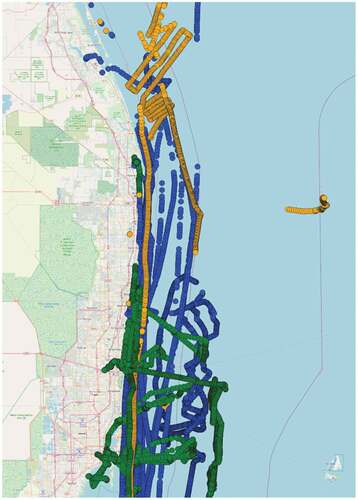
The data cleaning process involved removing duplicates with identical MMSI, date, and time entries. Other records were removed based on invalid SOG values. The latitude and longitude values were rounded to ${10}^{-4}$ which represents a precision of $10$ meters and each trajectory is defined as a set of observations over time with the same MMSI. 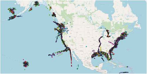Trajectories with less than $100$ observations were discarded, and the data was normalized before applying the auto-regression models.³ Figure 2 illustrates the $2,296\left[100,3000\right]$ trajectories that were analyzed after the preprocessing stage.⁴

Figure 2. The 2,296 fishing vessel trajectories selected for analysis.

ARIMA parameter analysis

The parameters $\left(p,d,q\right)$ were predetermined so that the same number of coefficients were produced for each of the modeled trajectories. To determine these parameter values, different $\left(p,d,q\right)$ configurations were tested for $289$ randomly selected MMSIs during April of 2020. The ARIMA parameters used in Equation 4 were selected from the following ranges: $p\to \left[1,3\right]$, $q\to \left[0,3\right]$, and $d\to \left[0,1\right]$, producing a total of $24$ different ARIMA configurations.

A model was created for both the latitude and the longitude for each trajectory in the dataset and the mean squared error (MSE) was calculated. The average and standard deviation of the MSE for each trajectory model was calculated to help determine a suitable combination of parameter values. The smaller the MSE value, the better the model represents the trajectory being analyzed. Figure 3 contains the box-plots for the MSE values of different ARIMA model parameters. The top and bottom plots illustrate the results for latitude and longitude respectively.⁵

Figure 3. Boxplot for each configuration of ARIMA parameters, where the top plot represents the latitude, and bottom plot represents longitude. (a) Latitude. (b) Longitude.

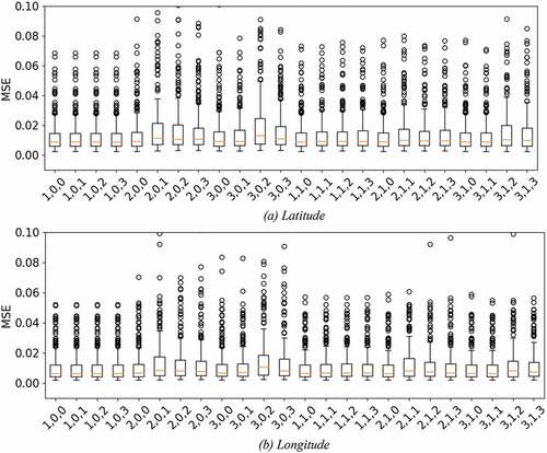
Based upon the MSE average and standard deviation, the parameters for the ARIMA model were selected to be $\left(p,d,q\right)\to \left(1,0,3\right)$, which had the lowest values for the MSE. It should be noted that the parameter representing the $AR$ process in ARIMA was $1$, which corresponds to the OU process used to predict vessel trajectories in reference (d’Afflisio, et al. 2018a).

Experiments

As previously described, this work uses the DCAIS dataset to analyze the behavior of fishing vessels in April of 2020. The preprocessing stage described in Section Dataset was applied and $2,296$ trajectories with unique MMSIs were analyzed. These trajectories are illustrated in Figure 2.

Next, ARIMA and the OU processes were used to model the behavior of each vessel using the latitude and longitude. These processes will fit a function that describes the latitude and the longitude of the vessel and will provide function coefficients for each modeled trajectory, or vessel. The coefficients are concatenated into a single vector to represent the movement behaviors. The Euclidean distance was calculated between the trajectory coefficients to create the distance matrix, which represents the similarity between vessel behaviors. The proposed analysis uses the distance matrix to perform the clustering analysis. Such an analysis aims to identify groups of vessels with similar behaviors and patterns within the trajectory.⁶ The graphics in Figure 4 illustrate the distance matrices for the ARIMA and OU processes, respectively. The axes represent the vessel trajectories, while the color represents the distance. The darker the color (blue) the more similar those trajectories are. As a result, the diagonal represents the distance between identical trajectories which are illustrated by the dark coloring used in this graphic.

Figure 4. This shows the distance between trajectories generated using the model coefficients respectively for both the ARIMA and OU processes. (a) ARIMA. (b) OU.

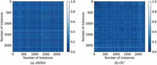
Given that all trajectories are formed using fishing vessel data, one would expect the vessels to exhibit similar behaviors, leading to small distance values in the similarity matrix. Observing the distance matrices in Figure 4, both the ARIMA and OU processes generate mostly small distance values as expected. This shows that these auto-regressive techniques can be a useful tool in analyzing the behavior of vessel trajectories.

Clustering methods

To identify patterns and outliers that represent anomalous vessel behavior, DBSCAN, HC, and SC were performed on the ARIMA and OU distance matrices. In this analysis, the DBSCAN method identifies the outliers based on the features, which differs from HC and SC which provide only the groups formed. Therefore, in the case of HC and SC, trajectories labeled as outliers were identified based on their silhouette measure. A low silhouette measure indicates that a vessel exhibits different behavior patterns than the other trajectories assigned to the clusters. To determine the number of outliers, a threshold for the silhouette measure was selected to be three times the standard deviation for this measure.

In the DBSCAN analysis, the minimum number of instances needed to define a cluster was empirically set to $m=3$, and the elbow technique was used to select $\epsilon$ which was $0.1$ and $0.02$ for the ARIMA and OU processes, respectively. For HC, the average-linkage measure was used to determine the inter-cluster distance, and in order to analyze the detected patterns on each hierarchical level, the number of clusters selected included: $2$, $5$, $10$, $15$. In the case of SC, the number of eigenvectors used was empirically chosen to be $k=3$, and the number of clusters set to $3$, which was chosen based on the silhouette measure. Table 1 contains the methods, the number of clusters, the number of outliers detected, and the silhouette measure when applicable.

Table 1. Table showing the methods, the number of clusters, the number of outliers detected, and the silhouette measure when applicable.

Features	Clustering	$k$	Outliers	Silhouette
ARIMA	DBSCAN	$1$	$28$	-
OU	DBSCAN	$12$	$56$	-
ARIMA	HC	$2$	$24$	$0.7994$
OU	HC	$2$	$21$	$0.8271$
ARIMA	HC	$5$	$87$	$0.5762$
OU	HC	$5$	$33$	$0.6209$
ARIMA	HC	$10$	$56$	$0.4293$
OU	HC	$10$	$35$	$0.4808$
ARIMA	HC	$15$	$15$	$0.4554$
OU	HC	$15$	$32$	$0.4888$
ARIMA	SC	$3$	$5$	$0.4177$
OU	SC	$3$	7	$0.5251$

Moreover, the similarity between each configuration was analyzed using the Adjusted Rand Index (ARI), which is a well-known metric that compares two clustering results (Vinh, Epps, and Bailey 2010). Such results was presented in Table 2, in which HC was executed with $15$ clusters and SC with $3$.

Table 2. Table showing the ARI measure between configurations executed, in which HC was executed with $15$ clusters and SC with $3$. In this table, AR represents ARIMA and DB corresponds to DBSCAN.

	AR/DB	AR/HC	AR/SC	OU/DB	OU/HC	OU/SC
AR/DB	$1$	$0.075$	$0.022$	$0.013$	$0.006$	$0.001$
AR/HC	$0.075$	$1$	$0.47$	$0.024$	$-0.012$	$0.001$
AR/SC	$0.022$	$0.47$	$1$	$0.072$	$-0.029$	$0.022$
OU/DB	$0.013$	$0.024$	$0.072$	$1$	$0.304$	$0.274$
OU/HC	$0.006$	$-0.012$	$-0.029$	$0.304$	$1$	$0.491$
OU/SC	$0.001$	$0.001$	$0.022$	$0.274$	$0.491$	$1$

From these results, clusters produced using the OU process have a higher silhouette value than the ones obtained with ARIMA. Such an observation implies that OU coefficients present a better separability of the patterns, i.e. provide less overlap between groups. Additionally, the low ARI values confirm that OU and ARIMA produced different models and features for the trajectories. On the other hand, the highest values of ARI suggest that different clustering algorithms may detect similar patterns when using the same AR model.

Visual analysis

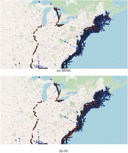
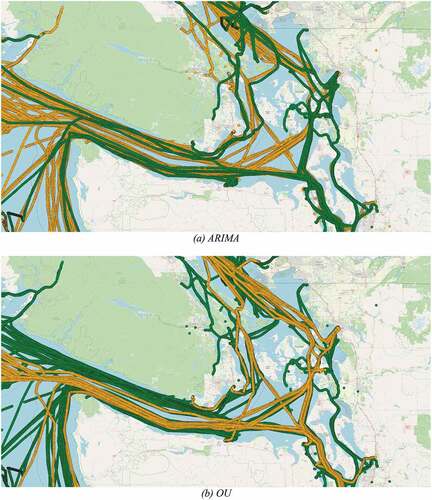
Vessel trajectories labeled as outliers are assumed to exhibit abnormal behavior because they are not in accordance with the norms represented by the established clusters. Some trajectories were labeled as outliers by both analyses using the ARIMA and OU processes. For example, when both modeling techniques were clustered with DBSCAN vessels that were fishing in rivers were labeled as outliers as shown in Figure 5. This result was due to the fact that the vessel behavior in a river differs from vessels that fish on the ocean.

Figure 5. Illustration of outliers detected by DBSCAN using both OU and ARIMA models. Both detected fishing vessel trajectories in rivers. (a) ARIMA. (b) OU.

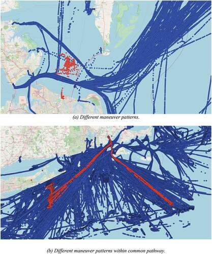
However, due to the differences in how the trajectories were modeled, many of the assigned outliers for both approaches were not the same. DBSCAN with ARIMA identified outliers as vessels that were not moving or exhibited abnormal movement patterns. Such behavior is illustrated in Figure 6(a) where the red trajectory is detected as an outlier as it presents chaotic movements that differ from the common pathway followed by most vessels. In addition, Figure 6(b) illustrates an outlier trajectory in red that shows movement patterns that differ from the others within the common pathway.

Figure 6. These figures show the outliers detected by DBSCAN using ARIMA, in which (a) the outlier does several maneuvers in the same location, and (b) the outlier presents different maneuver patterns in a common pathway. (a) Different maneuver patterns. (b) Different maneuver patterns within common pathway.

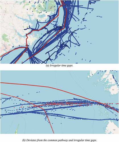
On the other hand, using DBSCAN with the OU process it was able to detect timing irregularities in vessel trajectories, i.e. AIS messages with irregular patterns and large time gaps between received messages. Such a detection is possible because OU receives temporal information to produce the model. Figure 7(a) illustrates these irregularities, in which the time gap between messages are inconsistent. Also, Figure 7(b) shows an outlier trajectory that follows an uncommon pathway, i.e. a pathway that is not followed by the other vessels.

Figure 7. These figures show the outliers detected by DBSCAN using ARIMA, in which (a) the outlier presents large gaps between messages where this behavior is not common, and (b) the outliers deviate from the common path and also irregular time gaps. (a) Irregular time gaps. (b) Deviates from the common pathway and irregular time gaps.

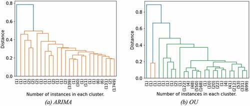
For HC, Figure 8 illustrates the dendrogram for both the ARIMA and OU processes. Some clusters in the dendrogram contain a small number of trajectories, which could mean that these clusters are composed of anomalies or are outliers, while clusters with a large number of trajectories are assumed to have similar behavior patterns. After examining the clusters that had a small number of trajectories and the outliers detected with the silhouette measure, it was determined that these trajectories are the same ones that DBSCAN classified as outliers. In addition, clustering configurations that used a small number of clusters typically produce one cluster containing most of the trajectories, while the others consist of $1$ or $2$ trajectories. As a result, $2$, $5$, $10$, and $15$ clusters were investigated.

Figure 8. Illustration of the dendrogram using the HC. (a) ARIMA. (b) OU.

HC allows for the exploration of different clustering combinations that contain trajectories with similar behaviors. Different levels of the hierarchical tree (dendrogram) can be explored to extract more information about vessel behavior patterns. In the deeper levels of the dendrogram, the clusters contain a reasonable number of instances ($>3$ instances), allowing for further analysis of the clusters to differentiate vessel movement patterns amongst the groups. Figure 9 shows an example of trajectories assigned to clusters in the same region when a total of $15$ clusters were used in the analysis. Although these trajectories go through the same paths or geographical regions, the clustering results produced using ARIMA differentiates based on the movement patterns, i.e. the trajectories in the green group present more turns and maneuvers than the yellow group. On the other hand, the application of the OU process seems to account for differences in direction, in which the green group is going west, and the yellow group is going east. These results show that HC may be used to analyze different patterns in vessel movements while identifying outliers.

Figure 9. Illustration of fishing vessel trajectories in a region clustered by HC using $15$ clusters. Figure (a) shows ARIMA results, in which trajectories in the green group present more turns and maneuvers than the yellow group. While, figure (b) presents OU. (a) ARIMA. (b) OU.

Lastly, SC with the OU process produced clusters based on region, which was not suitable to tackle the detection of anomalies. However, this confirms that OU models can represent spatio-temporal information. On the other hand, the combination of ARIMA and SC seems to segment groups based on movement and behavior as illustrated in Figure 10. This is seen by observing trajectories based on color where the blue cluster shows straight pathways, the yellow cluster corresponds to zigzag or more chaotic tracks, while the green cluster contains vessels with spiraled or circular movements.

Figure 10. Illustration of fishing vessel trajectories in a region clustered by SC using ARIMA. Blue cluster shows straight pathways, the yellow cluster corresponds to zigzag or chaotic tracks, and the green cluster contains vessels with spiraled or circular move.

In summary, ARIMA has the ability to capture vessels that are stationary or present a different pattern within common pathways. While the OU process identifies vessels that present irregularities in the time between messages. For instance, it detects large gaps of time between messages in a region where messages are received frequently with a short interval between them. In terms of clustering, DBSCAN is still a good approach to detect anomalies and outliers, but it fails to detect movement patterns. On the other hand, SC of the ARIMA models was able to detect different movement patterns which allows one to explore the behaviors of these fishing vessels. However, based on the visual analysis, this approach did not provide a well-defined analysis for outlier detection. Lastly, HC is a good approach to explore the vessels behavior as it provides different levels of clustering. By exploring these levels, it was possible to identify outliers that include: irregular time-gaps and different movement patterns within common and uncommon pathways. Additionally, it was possible to capture traffic patterns that include: the route direction and the number of maneuvers within the trajectory.

Conclusions

Research surrounding vessel trajectories typically makes use of unsupervised models in order to detect outliers based upon positional information. These approaches fail to detect anomalous behavior both in sparse regions of activity and along common traffic pathways. On the other hand, prediction methods that are used to detect anomalous behavior are only able to analyze single vessels at a particular instant of time. They are unable to analyze the anomalous behaviors associated with areas containing multiple vessels that may look normal unless one has specific guidance in terms of context or situational awareness. In addition, most datasets used in this domain are privately owned, making it difficult to reproduce scientific results.

Motivated by these gaps in the literature, this investigation utilizes the ARIMA and OU modeling techniques in order to generate similarity matrices that can be used to group vessels based on their behavior using clustering algorithms. As a result, the coefficients produced using the OU process were able to capture anomalous behaviors associated with observations having irregular time gaps between messages and routes that deviate from the norm. While the ARIMA process was able to detect stationary behaviors and abnormal patterns within common pathways. These results can be observed when using DBSCAN which also performed well at detecting outliers. However, DBSCAN essentially produced a single high-density cluster, lacking the representation of different behavior patterns.

On the contrary, the results obtained using the SC algorithm with the OU and ARIMA process suggest that SC was able to detect patterns using both models. When using the ARIMA process with SC, different vessel movement patterns were detected making it an appropriate approach to represent vessel behavior. However, when using the OU process, the clustering was influenced by the geographical location of the vessels, jeopardizing its ability to use movement behavior as a prominent feature. Also, the outliers detected with the silhouette measure for both models were not as meaningful as the outliers detected by DBSCAN because they do not present a different pattern from the other vessels in the same region.

In general, HC appears to be the most suitable clustering algorithm to explore movement patterns and detect outliers when using OU and ARIMA. The application of the HC algorithm to both modeling techniques produced one high-density cluster along with sparsely populated clusters. The smaller clusters contains trajectories that are the same as the outliers detected by DBSCAN. Also, both modeling techniques used with the HC algorithm produced different cluster shapes, detecting different types of movement patterns. In this scenario, the OU process divides the trajectories based on their directions, while ARIMA divided them based on the maneuver frequency (i.e. number of turns). Unlike others, the HC algorithm allows one to explore the similarities and differences in vessel behavior on a more granular level. Such an analysis is able to produce meaningful insights, supporting the detection of anomalous behavior between multiple vessels.

The analysis performed in this investigation demonstrates that the ARIMA and OU processes can be used to model the behavior of fishing vessels. The application of clustering techniques to these models is able to segregate vessels into groups that exhibit similarities in their movement patterns. The selection of the clustering approach depends on whether you are trying to identify specific vessel behaviors.

For future work, multivariate methods could be investigated to improve the modeling of trajectories. Such methods support the addition of other variables like speed and course, which may help capture different movement behaviors. For instance, with the OU process, the first derivative could be used to incorporate the velocity of the vessel into the model and applying the second derivative to incorporate the acceleration of the vessels. Moreover, to avoid adding artifacts to the clustering analysis due to the large errors provided by some models, future work may partition the data based upon local geographic regions prior to analysis. The analysis of a specific region should reduce the variability of the type of trajectories in the dataset by focusing on particular behaviors, making it easier to model vessel movement using the techniques explored in this analysis. Additionally, filtering methods should be incorporated to remove noise and help reduce errors. Lastly, feature selection will be explored to identify the most influential features for this type of analysis.

Acknowledgements

We would like to thank Anthony Isenor for reviewing this work and for his suggestions. Also, we thank Xiang Jiang for the helpful discussions. We acknowledge the support of the Natural Sciences and Engineering Research Council of Canada (NSERC), the CHIST-ERA grant CHIST-ERA-19-XAI-010, and NCN (grant No. 2020/02/Y/ST6/00064).

Disclosure statement

No potential conflict of interest was reported by the author(s).

Data availability statement

The data that support the findings of this study is openly available in the AIS Data for 2020 repository at https://coast.noaa.gov/htdata/CMSP/AISDataHandler/2020/index.html. In addition, the source code implemented to produce the results is available at https://github.com/marthadais/MovementAnalysis.

Additional information

Funding

This work was supported by the CHIST-ERA [CHIST-ERA-19-XAI-010]; Natural Sciences and Engineering Research Council of Canada [550722]; Narodowe Centrum Nauki [grant No. 2020/02/Y/ST6/00064].

Notes

1. The Wiener process is a real-valued continuous-time stochastic process used in physics to study Brownian Motion, the diffusion of minute particles suspended in fluids, and other types of diffusion problems (Üstünel 2006).

2. The dataset is available at https://coast.noaa.gov/htdata/CMSP/AISDataHandler/2020/index.html.

3. The latitude and longitude were divided by $90$ and $180$, respectively.

4. The number of messages composing each trajectory varies between $\left[100,36000\right]$, with most having around $7000$.

5. An MSE average of $0.01$ has an error of approximately $1000$ meters in terms of latitude and longitude.

6. The source code is available at https://github.com/marthadais/MovementAnalysis.

References

- Bagnall, A. J., and G. J. Janacek. 2004. “Clustering Time Series from ARMA Models with Clipped Data.” In Proceedings of the tenth ACM SIGKDD international conference on Knowledge discovery and data mining (KDD '04). Association for Computing Machinery, New York, NY, USA, 49–58. doi:10.1145/1014052.1014061.
- Coscia, P., P. Braca, L. M. Millefiori, F. A. N. Palmieri, and P. Willett. 2018. “Multiple Ornstein–Uhlenbeck Processes for Maritime Traffic Graph Representation.” IEEE Transactions on Aerospace and Electronic Systems (IEEE) 54: 2158–2170. doi:10.1109/TAES.2018.2808098.
- d’Afflisio, E., P. Braca, L. M. Millefiori, and P. Willett. 2018a. “Detecting Anomalous Deviations from Standard Maritime Routes Using the Ornstein–Uhlenbeck Process.” IEEE Transactions on Signal Processing (IEEE) 66: 6474–6487. doi:10.1109/TSP.2018.2875887.
- d’Afflisio, E., P. Braca, L. M. Millefiori, and P. Willett. 2018b. “Maritime Anomaly Detection Based on mean-reverting Stochastic Processes Applied to a real-world Scenario.” In 2018 21st International Conference on Information Fusion (FUSION), Cambridge, UK, 1171–1177. IEEE.
- Ester, M., H.-P. Kriegel, J. Sander, X. Xiaowei. 1996. “A density-based Algorithm for Discovering Clusters in Large Spatial Databases with Noise.” kdd 96 (34): 226–231.
- Forti, N., L. M. Millefiori, and P. Braca. 2019. “Unsupervised Extraction of Maritime Patterns of Life from Automatic Identification System Data.” In OCEANS, Marseille, France, 1–5. IEEE.
- Forti, N., L. M. Millefiori, P. Braca, and P. Willett. 2019. “Anomaly Detection and Tracking Based on mean–reverting Processes with Unknown Parameters.” ICASSP 2019-2019 IEEE International Conference on Acoustics, Speech and Signal Processing (ICASSP), Brighton, UK, 8449–8453.
- Forti, N., L. M. Millefiori, P. Braca, and P. Willett. 2021. “Bayesian Filtering for Dynamic Anomaly Detection and Tracking.“ In IEEE Transactions on Aerospace and Electronic Systems 58 (3): 1528–1544. doi:10.1109/TAES.2021.3122888.
- Gloaguen, P., S. Mahévas, E. Rivot, M. Woillez, J. Guitton, Y. Vermard, and M.-P. Etienne. 2015. “An Autoregressive Model to Describe Fishing Vessel Movement and Activity”. Environmetrics Wiley Online Library 26: 17–28. doi:10.1002/env.2319.
- Guo, S., J. Mou, L. Chen, and P. Chen. 2021. “An Anomaly Detection Method for AIS Trajectory Based on Kinematic Interpolation.” Journal of Marine Science and Engineering, no. 6: 609. doi:10.3390/jmse9060609.
- Hendrawati, T., A. H. Wigena, I. M. Sumertajaya, and B. Sartono. 2021. “Clustering of Commodity Inflation Pattern Based on Estimated ARIMA Model.” In Journal of Physics: Conference Series, Bogor, Indonesia, 012058. IOP Publishing.
- Huang, J., F. Zhu, Z. Huang, J. Wan, and Y. Ren. 2021. “Research on Real-Time Anomaly Detection of Fishing Vessels in a Marine Edge Computing Environment.” Mobile Information Systems 2021: 1–15. doi:10.1155/2021/5598988.
- Hyndman, R. J., and G. Athanasopoulos. 2021. “Forecasting: Principles and Practice, 3rd edition.” Melbourne, Australia: OTexts. Accessed on August 31, 2022. OTexts.com/fpp3
- Ismail, A., and A. Vigneron. 2015. “A New Trajectory Similarity Measure for GPS Data.” Proceedings of the 6th ACM SIGSPATIAL International Workshop on GeoStreaming, Bellevue, WA, USA, 19–22.
- Jiang, H., W. U. Yao, L. Y. U. Kuilin, and W. A. N. G. Huijiao. 2019. “Ocean Data Anomaly Detection Algorithm Based on Improved k-medoids.” 2019 Eleventh International Conference on Advanced Computational Intelligence (ICACI), Guilin, China, 196–201.
- Kalpakis, K., D. Gada, and V. Puttagunta. 2001. “Distance Measures for Effective Clustering of ARIMA time-series.” In Proceedings 2001 IEEE international conference on data mining, San Jose, CA, USA, 273–280. IEEE.
- Karatas, G. B., P. Karagoz, and O. Ayran. 2021. “Trajectory Pattern Extraction and Anomaly Detection for Maritime Vessels.” Internet of Things 16: 100436. Elsevier.
- Kontopoulos, I., I. Varlamis, and K. Tserpes. 2021. “A Distributed Framework for Extracting Maritime Traffic Patterns.” International Journal of Geographical Information Science 35: 767–792. doi:10.1080/13658816.2020.1792914.
- Laxhammar, R. 2008. “Anomaly Detection for Sea Surveillance.“ 11th International Conference on Information Fusion, Cologne, Germany, 1-8.
- Lee, J.-G., J. Han, and K.-Y. Whang. 2007. “Trajectory Clustering: A partition-and-group Framework.” Proceedings of the 2007 ACM SIGMOD international conference on Management of data, Beijing, China, 593–604.
- Li, H., J. Liu, W. Kefeng, Z. Yang, R. Wen Liu, and N. Xiong. 2018. “Spatio-temporal Vessel Trajectory Clustering Based on Data Mapping and Density.” IEEE Access (IEEE) 6: 58939–58954. doi:10.1109/ACCESS.2018.2866364.
- Li, H., J. Liu, R. Wen Liu, N. Xiong, W. Kefeng, and T.-H. Kim. 2017. “A Dimensionality reduction-based multi-step Clustering Method for Robust Vessel Trajectory Analysis.” Sensors (Multidisciplinary Digital Publishing Institute) 17: 1792.
- Liang, M., R. Wen Liu, L. Shichen, Z. Xiao, X. Liu, and L. Feng. 2021. “An Unsupervised Learning Method with Convolutional auto-encoder for Vessel Trajectory Similarity Computation.” Ocean Engineering 225: 108803.
- Liu, B., E. N. de Souza, S. Matwin, and M. Sydow. 2014. “Knowledge-based Clustering of Ship Trajectories Using density-based Approach.” 2014 IEEE International Conference on Big Data (Big Data), Washington, DC, USA, 603–608.
- Liu, R. W., J. Nie, S. Garg, Z. Xiong, Y. Zhang, and M. Shamim Hossain. 2020. “Data-driven Trajectory Quality Improvement for Promoting Intelligent Vessel Traffic Services in 6G-enabled Maritime IoT Systems.“ IEEE Internet of Things Journal 8 (7): 5374–5385. doi:10.1109/JIOT.2020.3028743.
- Logan, J. D., and W. Wolesensky. 2009. Mathematical Methods in Biology. Vol. 96. Toronto, ON, CA: John Wiley & Sons.
- Luo, T., X. Zheng, X. Guangluan, F. Kun, and W. Ren. 2017. “An Improved DBSCAN Algorithm to Detect Stops in Individual Trajectories.” ISPRS International Journal of Geo-Information (Multidisciplinary Digital Publishing Institute) 6: 63. doi:10.3390/ijgi6030063.
- Magdalene, J. J. C., and B. S. E. Zoraida. 2022. “Predicting the Usage of Energy in a Smart Home Using Improved Weighted K-Means Clustering ARIMA Model.” JOURNAL OF ALGEBRAIC STATISTICS 13: 1770–1777.
- Mascaro, S., A. E. Nicholso, and K. B. Korb. 2014. “Anomaly Detection in Vessel Tracks Using Bayesian Networks.” International Journal of Approximate Reasoning 55: 84–98. doi:10.1016/j.ijar.2013.03.012.
- Mazzarella, F., M. Vespe, A. Alessandrini, D. Tarchi, G. Aulicino, and A. Vollero. 2017. “A Novel Anomaly Detection Approach to Identify Intentional AIS on-off Switching.” Expert Systems with Applications (Elsevier) 78: 110–123. doi:10.1016/j.eswa.2017.02.011.
- Murray, B., and L. Prasad Perera. 2022. “Ship Behavior Prediction via Trajectory extraction-based Clustering for Maritime Situation Awareness.” Journal of Ocean Engineering and Science 7: 1–13. doi:10.1016/j.joes.2021.03.001.
- Newaliya, N., and Y. Singh. 2021. “A Review of Maritime Spatio-temporal Data Analytics.” In 2021 International Conference on Computational Performance Evaluation (ComPE), Shillong, India, 219–226. IEEE.
- Ng, A., M. Jordan, and Weiss, Y. 2001. “On spectral clustering: Analysis and an algorithm.” In Advances in neural information processing systems 14.
- Nguyen, D., R. Vadaine, G. Hajduch, R. Garello, and R. Fablet. 2021. “GeoTrackNet–A Maritime Anomaly Detector Using Probabilistic Neural Network Representation of AIS Tracks and A Contrario Detection.“ IEEE Transactions on Intelligent Transportation Systems 23 (6): 5655–5667. doi:10.1109/TITS.2021.3055614.
- Nielsen, F. 2016. “Hierarchical Clustering.” In Introduction to HPC with MPI for Data Science Undergraduate Topics in Computer Science, 195–211. Cham, Germany: Springer.
- Pallotta, G., M. Vespe, and K. Bryan. 2013. “Vessel Pattern Knowledge Discovery from AIS Data: A Framework for Anomaly Detection and Route Prediction.” Entropy (Multidisciplinary Digital Publishing Institute) 15: 2218–2245.
- Patmanidis, S., I. Voulgaris, E. Sarri, G. Papavassilopoulos, and G. Papavasileiou. 2016. “Maritime Surveillance, Vessel Route Estimation and Alerts Using AIS Data.” 2016 24th Mediterranean Conference on Control and Automation (MED), Athens, Greece, 809–813.
- Peiguo, F., H. Wang, K. Liu, H. Xiaohui, and H. Zhang. 2017. “Finding Abnormal Vessel Trajectories Using Feature Learning.” IEEE Access (IEEE) 5: 7898–7909. doi:10.1109/ACCESS.2017.2698208.
- Riveiro, M., G. Falkman, and T. Ziemke. 2008. “Visual Analytics for the Detection of Anomalous Maritime Behavior.” 2008 12th International Conference Information Visualisation, London, UK, 273–279.
- Riveiro, M., G. Pallotta, and M. Vespe. 2018. “Maritime Anomaly Detection: A Review.” Wiley Interdisciplinary Reviews. Data Mining and Knowledge Discovery 8: e1266.
- Rong, H., A. P. Teixeira, and C. Guedes Soares. 2020. “Data Mining Approach to Shipping Route Characterization and Anomaly Detection Based on AIS Data.” Ocean Engineering 198: 106936.
- Ross, S. M. 2014. Introduction to Probability Models 11 ed. Washington, DC: Academic press.
- Rousseeuw, P. J. 1987. “Silhouettes: A Graphical Aid to the Interpretation and Validation of Cluster Analysis.” Journal of Computational and Applied Mathematics (Elsevier) 20: 53–65. doi:10.1016/0377-0427(87)90125-7.
- Shahir, H. Y., U. Glasser, A. Yaghoubi Shahir, and H. Wehn. 2015. “Maritime Situation Analysis Framework: Vessel Interaction Classification and Anomaly Detection.” In 2015 IEEE International Conference on Big Data (Big Data), Santa Clara, CA, USA, 1279–1289. Ieee.
- Stella, X. Y., and J. Shi. 2003. “Multiclass Spectral Clustering.” Proceedings Ninth IEEE International Conference on Computer Vision, Nice, France, 1: 313–319. doi:10.1109/ICCV.2003.1238361.
- Tadayon, M., and Y. Iwashita. 2020. “A Clustering Approach to Time Series Forecasting Using Neural Networks: A Comparative Study on distance-based Vs. feature-based Clustering Methods.“ arXiv preprint arXiv:2001.09547.
- Üstünel, A. S. 2006. An Introduction to Analysis on Wiener Space. cham, switzerland: Springer.
- Vinh, N. X., J. Epps, and J. Bailey. 2010. “Information Theoretic Measures for Clusterings Comparison: Variants, Properties, Normalization and Correction for Chance.” The Journal of Machine Learning Research 11: 2837–2854.
- Watson, J. R., and J. Woodil. 2019. “Anticipating Illegal Maritime Activities from Anomalous Multiscale Fleet Behaviors Measured from Space.” arxiv preprint arXiv:1910.05424.
- Xiao, Z., L. Zhang, F. Xiuju, W. Zhang, J. Tianyi Zhou, and R. Siow Mong Goh. 2019. “Concurrent Processing Cluster Design to Empower Simultaneous Prediction for Hundreds of Vessels’ Trajectories in near real-time.“ IEEE Transactions on Systems, Man, and Cybernetics: Systems 51 (3): 1830–1843. doi:10.1109/TSMC.2019.2906381
- Yao, D., C. Zhang, Z. Zhu, J. Huang, and B. Jingping 2017. “Trajectory Clustering via Deep Representation Learning.” 2017 international joint conference on neural networks (IJCNN), Anchorage, AK, USA.
- Zhao, L., and G. Shi. 2019. “Maritime Anomaly Detection Using density-based Clustering and Recurrent Neural Network.” The Journal of Navigation 72: 894–916. doi:10.1017/S0373463319000031.