A machine learning-based dynamic ensemble selection algorithm for microwave retrieval of surface soil freeze/thaw: A case study across China

ABSTRACT

The surface soil freeze/thaw (FT) cycle serves as a “switch” for land surface processes; accurate retrieval of surface FT dynamics based on satellite passive microwave remote sensing is critical for studies on climate change and dynamics of the cryosphere. This study aims to improve FT retrieval accuracy by developing a new FT retrieval algorithm that applies the K-Nearest Oracle Union (KNORA-UNION) dynamic ensemble selection algorithm. This algorithm can optimally integrate three machine learning models on a grid cell scale, namely Random Forests, Extra-Trees, and Extreme Gradient Boosting. We applied our developed freeze/thaw dynamic ensemble selection retrieval algorithm (FT-DESA) to retrieve China’s daily surface FT states from 2009 to 2020 based on multiband Special Sensor Microwave Imager/Sounder (SSMIS) brightness temperatures. We then evaluated our FT-DESA results by comparing the observations of 2398 stations and three other existing FT algorithms, including the modified seasonal threshold algorithm (MSTA), decision tree algorithm (DTA), and dual-index algorithm (DIA) across China. Our results show that FT-DESA has the highest retrieval accuracy and the lowest biases across China among the four algorithms. The mean classification accuracy for the PM and AM overpasses of FT-DESA is 89% and 84%, respectively. The evaluations further indicate that some of the existing algorithms do not reflect the temporal and spatial heterogeneity in selecting thresholds for FT classification. This study demonstrates that the freeze/thaw dynamic ensemble selection algorithm can provide daily estimates of surface FT states across China, improve FT states’ retrieval accuracy, and provide a valuable multi-decadal record for daily FT states.

KEYWORDS:

• Freeze/thaw
• dynamic ensemble selection algorithm
• China
• passive microwave remote sensing

1. Introduction

Approximately 60% of near-surface soils worldwide experience seasonal phase transitions between water and ice every year (Kim et al. 2011). Changes in the timing, spatial extent, and duration of surface soil freeze/thaw (FT) are sensitive to climate change and can serve as an climate change indicator (Zhang, Armstrong, and Smith 2003b). Surface FT processes significantly affect land hydrology, crop growth, carbon dynamics, and the energy exchange between the Earth and the atmosphere (Zhang and Armstrong 2001). Surface FT cycles also have a substantial impact on ecosystem function. The number of thawed days directly affects the interannual variability and spatial distribution of net primary productivity (Kim et al. 2012) and net ecosystem carbon exchange (Zhang, Armstrong, and Smith 2003b). Recently, changes in FT processes have caused increasing nitrogen emissions in permafrost regions (Schuur, Abbott, and Network 2011; Wang et al. 2017). Monitoring the FT state is critical for studying the Earth’s hydrologic and surface temperature patterns and dynamics (Wang et al. 2020).

Prior to the satellite era, traditional methods for determining the surface soil FT state relied on numerical simulations extrapolated from a point to a larger area using limited ground measurement sources. These traditional methods are time-consuming and usually display considerable uncertainty. Leveraging the launches of the Scanning Multichannel Microwave Radiometer (SMMR; operational from 1978 to 1987), the Special Sensor Microwave Imager (SSM/I; operational from 1987 to the present), the Advanced Microwave Scanning Radiometer-EOS (AMSR-E; operational from 2002 to 2011), and the Special Sensor Microwave Imager/Sounder (SSMIS; operational from 2000 to the present) among other satellite missions, we have obtained continuous records of global passive microwave brightness temperatures (T_b) for over 40 years. A large number of experimental studies have shown that frozen soil has a low T_b of 37 GHz, and the gradient between low-frequency brightness temperature and high-frequency brightness temperature (spectral gradient) of frozen soil is negative because of the darkening of the bulk scattering, while the opposite is true for thawed soil (England, Galantowicz, and Zuerndorfer 1991; Jin, Li, and Che 2009; Kim et al. 2017; McFarland, Miller, and Neale 1990; Zhang et al. 2003a; Zhang and Armstrong 2001; Zuerndorfer and England 1992). The thresholds of the 37 GHz T_b and the spectral gradient between 18/19 GHz and 37 GHz T_b to distinguish the FT states can be determined through statistical analysis of the samples. These passive T_b observations are suitable for detecting surface soil moisture and FT cycles over long time series and from regional to global scales (Zhang et al. 2019). Thus, satellite remote sensing provides a critical data resource for overcoming the issues associated with mapping geographical features solely from field data (Shirmard et al. 2022). Moreover, in recent years, the progress in computing power and the development of machine learning have enabled scientists to solve problems existing in traditional methods (Merchant et al. 2022; Shirmard et al. 2022). As a subfield of artificial intelligence, machine learning has been proven to be effective and reliable because it can efficiently and accurately analyze and classify remote sensing images (Maxwell, Warner, and Fang 2018; Merchant et al. 2022; Wang et al. 2019b).

In the last two decades, a long time series of remote sensing products devoted to the surface FT state has been publicly released and applied to studies on climate change and vegetation dynamics. For example, the modified seasonal threshold algorithm (MSTA) is an improved version of the seasonal threshold algorithm, treating the T_b thresholds as a variable that changes in space and time (Kim et al. 2017). Algorithms based on the polarization ratio (PR) require more microwave remote sensing data to derive the FT reference values (Rautiainen et al. 2014, 2016; Roy et al. 2015, 2017b). Based on the AMSR-E and AMSR2 passive microwave data, Zhao et al. (2011) derived a global near-surface FT state through a discriminant algorithm. There are also long time series surface FT data sets in China, which are mainly obtained by multi-channel bright temperatures through the double-index FT classification algorithm (Jin et al. 2015) and a decision tree algorithm (Jin, Li, and Che 2009). Most satellite FT algorithms only consider the surface FT state at the time of descending orbits. However, surface FT events may occur within one day at the beginning of spring and the end of autumn. These intra-day FT cycles are more sensitive to climate change but are often ignored in studies (Kim et al. 2011). The disturbance caused by deserts should also be excluded from the FT classification. These are usually large areas with complex surfaces with scattering characteristics similar to frozen surfaces, so they could be mistakenly classified as frozen soil (Jin, Li, and Che 2009). Although some emerging machine learning models have been used to derive the FT state, they still lack an integrated method that can utilize multiple machine learning models to enhance the accuracy and reliability of the data-driven satellite FT retrieval.

Therefore, we developed a new satellite-based freeze/thaw dynamic ensemble selection retrieval algorithm (FT-DESA) through the domain-specific application of a dynamic ensemble selection algorithm, which can jointly utilize multiple machine learning models and optimally integrate these models on a grid cell-by-grid cell scale to derive the surface FT state. To fully take advantage of the freeze-thaw data (both AM and PM overpasses) measured by the spaceborne radiometers, we produced an observation-based baseline data set, which is composed of the ground observations at the local times close to those of the AM and PM overpasses. The surface state is classified into five classes: frozen (frozen in both AM and PM), thawed (thawed in both AM and PM), transitional (frozen in AM and thawed in PM), inverse transitional (thawed in AM and frozen in PM), and desert, by integrating the information of ascending and descending orbits. The FT-DESA algorithm can quickly and accurately classify the surface FT state according to the characteristics of different regions and fill the gap in the surface FT state in high-altitude regions with no observed data in China.

Moreover, we verify the accuracy of the FT-DESA algorithm based on a comparative analysis with three other existing satellite FT retrieval/classification algorithms. The FT products from MSTA (Kim et al. 2017), decision tree algorithm (DTA) (Jin, Li, and Che 2009), dual index algorithm (DIA) (Jin 2016), and our algorithm were assessed against the measured soil temperature at the topsoils of 2398 stations in China.

2. Data and methods

2.1 Data

2.1.1 Brightness temperature

The T_b data used in this study were derived from the SSMIS. The SSMIS is a passive microwave radiometer with 24 channels designed to obtain multiple polarized surfaces and atmospheric temperatures, soil moisture, and land variables under different weather conditions. The channel frequencies of the SSMIS span from 19 GHz to 183 GHz. In addition, SSMIS replaced the 85.5 GHz channel on the SSM/I with a 91.655 GHz channel and only has a vertically polarized mode for the 22.2 GHz channel. All other frequencies were simultaneously captured in both the horizontal and vertical polarizations simultaneously. The ascending local time of SSMIS is 17:31, while the descending local time of SSMIS is 5:31. More information on the SSMIS can be found in Bommarito (1993).

In this study, T_b data on the Northern Hemisphere EASE-GRID from 2009 to 2020 were downloaded from Remote Sensing Systems (http://www.remss.com/). To produce a spatiotemporally continuous T_b record, we filled the missing values resulting from orbital gaps through a temporal linear interpolation using the neighboring T_b values and a 7-day sliding window, following the 6-day sliding window method (Jin et al. 2015).

2.1.2 Observed ground temperature

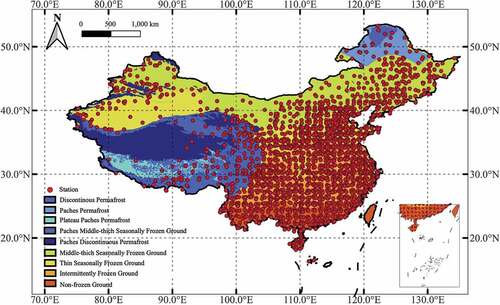
Observed ground temperature (T_g) data were obtained from the Daily Data Set of Basic Meteorological Elements of National Surface Meteorological Stations in China (V3.0) released by the National Tibetan Plateau Data Center (https://data.tpdc.ac.cn/), which provides daily ground surface temperature data from 2009 to 2016 at 2398 meteorological stations in China, including basic meteorological stations, benchmark climate stations, and general meteorological stations (National Meteorological Information 2019). These stations span a spatial extent from 16.32° N to 52.58° N and from 75.14° E to 132.58° E (Figure 1). The ground temperature used in this study was measured using a white mercury ball thermometer with a diameter of ~3 mm, which is partially buried to limit the influence of radiation and air (Wang, Zhang, and Zhong 2015).

Figure 1. Map of permafrost types and locations of ground temperature stations used in this study across China. The 2398 red points represent the ground surface temperature stations.

2.1.3 Land-use map

Areas covered by deserts were extracted from the land-use map of China for 2015 (Chinese Academy of Sciences and Environmental Science Data 2019). Based on many major research projects such as the National Science and Technology Support Program and the Knowledge Innovation Project of the Chinese Academy of Sciences, the Land Use Status Monitoring Database of China is a multitemporal land-use database covering China’s land areas. This dataset uses Landsat TM/ETM images for each period with the aid of manual visual interpretation. Further descriptions of this dataset can be found on the Resource and Environment Science and Data Center (http://www.resdc.cn/).

2.1.4 Permafrost classification map

The permafrost classification map in China (Figure 1) was compiled by Li, Nan, and Zhou (2012) on the basis of other existing observation-based permafrost maps of China and ground surveys (http://www.resdc.cn/).

2.1.5 Independent FT Products

In this study, surface soil FT records produced by the MSTA algorithm (2009–2015) released by the American Snow and Ice Data Center (https://nsidc.org) with a single index algorithm (Kim et al. 2017), the DTA algorithm, and the DIA algorithm (2009–2015) released by the National Tibetan Plateau Data Center (https://data.tpdc.ac.cn/) (Jin et al. 2015) were selected for comparison with our FT classification results. All four FT records were compared with the station observations. Because the original timespan for the FT records based on the decision tree algorithm is only up to 2008, we adopted the same algorithm driven by the same variables, such as the scattering index, T_b37V, and polarization difference at 19 GHz to drive the DTA FT records from 2009 to 2015. Desert areas were also classified based on this algorithm (Jin, Li, and Che 2009).

2.2 Methodology

2.2.1 Freeze/thaw dynamic ensemble selection algorithm

Ensemble learning is a new machine-learning paradigm that trains multiple classifiers first, and then integrates the trained classifiers to complete the learning task with a fusion strategy (Dietterich 2000). This method is also called a multi-classifier system. It has become a research hotspot in the machine learning field since the 1990s because it can substantially improve the generalizability of a learning system (Renner 2000). Static ensemble selection, dynamic classifier selection, and dynamic ensemble selection are the three schemes used to select and combine classifiers (Zhu 2019). Dynamic ensemble selection strategies denote the techniques that select an ensemble of classifiers instead of a single one (Błaszczyk and Jȩdrzejowicz 2021). These methods select a group of base classifiers that reaches the minimum competence level to form the classifier ensemble. Several studies have proven that a dynamic ensemble selection scheme can outperform the static ensemble selection methods (Cruz, Sabourin, and Cavalcanti 2018; Ye and Dai 2018). Moreover, selecting a set of classifiers can reduce the risk of overgeneralization by selecting only a single classifier (Ko, Sabourin, and Britto 2008).

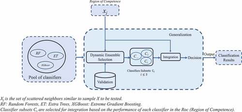
The k-nearest-oracles union (KNORA-UNION) dynamic ensemble selection algorithm is a dynamic ensemble method based on a linear random oracle (Kuncheva and Rodriguez 2007). The concept of KNORA-UNION is similar to those of the overall local accuracy method (OLA), local class accuracy method (LCA), a priori selection method (A Priori), and a posteriori selection method (A Posteriori) in their consideration of the nearest neighbors of test samples. However, KNORA-UNION is different from the other algorithms because of the region’s direct use of training samples to find the best ensemble for a given sample (Kuncheva and Rodriguez 2007). KNORA-UNION can find the nearest neighbors of any test data point in the validation set, sort out the classifiers that successfully classify those neighbors in the validation set, and then use them to compose the ensemble to classify the given pattern in the test set (Ko, Sabourin, and Britto 2008).

We applied the KNORA-UNION algorithm in the freeze/thaw retrieval field called the freeze/thaw dynamic ensemble selection algorithm (FT-DESA). The KNORA-UNION was implemented using Python software version 3.8 with the package “deslib” (Cruz et al. 2020). The KNORA-UNION framework is divided into three parts: (1) generation of a classifiers pool. Pool generation involves producing a set of diverse and accurate classifiers, maintaining diversity through a heterogeneous ensemble pool of different bare classifiers, or a homogenous ensemble pool of bagging, boosting, or hybrid schemes (Britto, Sabourin, and Oliveira 2014). This study selected three machine learning models, Random Forests, Extra-Trees, and Extreme Gradient Boosting (XGBoost), which have relatively high performance and accuracy in classification tasks (Fernández-Delgado et al. 2014; Zhang et al. 2021) and our experiments, as baseline models in the classifier pool. The labeled samples in the validation set are called the dynamic selection dataset (D_SEL) (Britto et al. 2014; Cruz et al. 2019). (2) Generation of the region of competence (ROC). The set of k-nearest neighbors in the D_SEL of the validation set is called the region of competence (ROC) (Britto et al. 2014; Cruz et al. 2019; Dos Santos, Sabourin, and Maupin 2008). Specifically, ROC mainly refers to collecting scattered samples that are similar to the samples tested in D_SEL. ROC was generated using the k-Nearest Neighbor (KNN) technique in the D_SEL. (3) Selection and integration of classifiers subsets based on the performance of each classifier in the classifier pool in ROC (Figure 2). The KNORA-UNION method measures the capability level of the base classifier based on the number of correctly classified instances within the defined capability range. Suppose that a test pattern X has K neighbors (x_j, 1 $\le$ j $\le$ K) and that its jth-nearest neighbor is correctly classified by a set of classifiers (C(j), 1 $\le$ j $\le$ K). Every classifier (c_i ∈ C(j)) of the correct classifier set C(j) should submit a vote on sample X. Because all the K-nearest neighbors of the test pattern X are considered, one should note that a classifier has more than one vote if it correctly classifies more than one neighbor. If a classifier correctly classifies more neighbors, it will have more votes for the test pattern (Figure 2). The votes of every selected base classifier, which are equal to the correctly predicted labels in the ROC, are combined to compose the ensemble (Dogo et al. 2021). Finally, the majority voting method was used for the integrated classification of the classification samples. The category with the most votes was the final prediction category of the samples to be classified.

Figure 2. Flowchart of the KNORA-UNION algorithm used in this study.

2.2.2 Data processing and model development

Selecting representative training samples is the basis for analyzing the radiant brightness and temperature characteristics of objects in different states and the premise for determining the threshold values of each station. Zheng et al. (2020) found that land surface temperature primarily controls the frozen ground types and frozen depth based on a synthetic dataset of the permafrost thermal state for the Tibetan Plateau (Zhao et al. 2021), which is reported as the first and currently the most comprehensive permafrost monitoring data set on the Tibetan Plateau. Moreover, some studies have found that the vertically polarized T_b at 37 GHz (T_b37V) is strongly linked to the surface air temperature and ground temperature at depths of less than 5 cm (Jin et al. 2015; Shao and Zhang 2020; Zhang, Armstrong, and Smith 2003b). Relative to the other choices, such as air temperature (Kim et al. 2011) and soil temperatures at different depths (Zwieback, Paulik, and Wagner 2015), the 0-cm ground temperature (T_g) can be a better choice for inferring the FT status because microwave remote sensing mainly observes the FT transitions of near-surface soil (Hu et al. 2017). Recent studies have demonstrated how to estimate freezing point depression in the lab and in situ (Pardo Lara et al. 2020) as well as how these estimates may be affected by the volume measured (Pardo Lara et al. 2021). However, in this study, freezing point depression was not considered for long-time and large-scale freeze/thaw retrieval. Freeze/thaw states were defined by the standard ground temperature observations threshold of 0°C. When T_g≆0°C, the near-surface soil is considered frozen; otherwise, the near-surface soil is considered in a thawed state. Moreover, the satellite data from the descending node (AM) and ascending node (PM) passes were found to be more closely related to daily minimum and maximum ground temperatures, respectively, than to the daily mean (Xie, Jin, and Yang 2013). Moreover, previous studies have shown that the minimum surface temperature (T_min) is the best indicator for calibrating the threshold of the 37 GHz bright temperatures in vertical polarization at the FT boundary, which can avoid the influence of wet snow (Jin, Li, and Che 2009; Zhang, Armstrong, and Smith 2003b). Desert is also a target for classification. In winter, owing to the effect of “volume scattering darkening,” the microwave radiation signal of the desert is very similar to that of the frozen surface, and the desert is easily misclassified. To exclude the influence of the main deserts in China on distinguishing the FT states, we randomly extracted the T_b values of 10 desert grid cells from the Taklimakan Desert based on the land-use maps of China as input samples. The ground temperature observation stations located in the desert grid cells were marked as deserts for training and validation.

Moreover, six spectral classification indices based on the SSMIS brightness temperatures were selected as the input of the classifiers in this study: T_b37V, 22 GHz brightness temperature in vertical polarization (T_b22V), scattering index (SI), polarization difference of the 19 GHz brightness temperatures (PD), spectral gradient (SG) between the 19 GHz and 37 GHz T_b, and the difference between T_B22V and T_B91V (T_B22V-T_B91V). T_b37V has been proven to be a good indicator of surface temperature variation (Chai et al. 2014; Kim et al. 2017). In this study, we also used T_b22V as another classification index, which is also a good indicator to distinguish between the freeze, thaw, and desert states (Li, Li, and Zhu 2012). SI represents the degree of deviation from the actual value of T_B85V caused by scattering. SI is mainly used to distinguish strong scatterers from weak scatterers and non-scatterers (Jin, Li, and Che 2009). Because the SSMIS satellite replaced the 85 GHz channel with the 91 GHz channel, we used the 91 GHz data instead of the 85 GHz data to calculate SI from 2009 to 2020 (Chai et al. 2014). The PD between T_B19V and T_B19H is mainly used to reflect the roughness of the surface. With an increase in the surface roughness, the coherent reflection component decreased, the diffuse scattering component increased, the emissivity tends to be independent of the polarization mode, and the polarization difference decreased. Therefore, this index can identify the desert with a relatively smooth surface, whose polarization difference is usually greater than 25 K. When the soil is frozen, the volume-scattering effect is obscured in the lower frequency channels, contributing to a negative spectral gradient (Zhao et al. 2011). Therefore, a combination of T_b37V and SG between 19 GHz and 37 GHz can determine whether the surface soils are frozen or not (Shao and Zhang 2020). The final classification index was T_B22V-T_B91V. Previous studies have shown that T_B22V-T_B85V (in this study, we used T_B91V instead of T_B85V, considering that the SSMIS satellite replaced the 85 GHz channel with the 91 GHz channel) serves as a critical indicator to distinguish between desert and permafrost (Li, Li, and Zhu 2012). These six indices all contribute to the model classification and can represent the differential physical characteristics of different ground states.

After all the samples were pre-processed to obtain their classification labels and indices, we trained them using the KNORA-Union dynamic ensemble selection algorithm. We selected the ground observation data in 2009 as the training samples because the training results in 2009 were relatively good with the completed ground temperature and brightness temperature datasets. In addition, the training data span an entire year and can well represent the seasonal and intra-annual variability. In 2009, 80% and 20% of the samples were randomly selected to train and validate the models, respectively. The validation set is used to decide when to stop training to avoid overfitting and determine whether the structure of the network is optimal. Moreover, ground observation data from 2010 to 2016 were selected for testing. The test set was used to evaluate the generalizability and predictability of the trained model (Fausett 2006). After model training, validation and testing, we further applied the trained model to predict the gridded FT state of China in the morning (descending orbit, i.e. AM orbit) and afternoon (ascending orbit, i.e. PM orbit) from 2009 to 2020. The resulting AM and PM FT classifications were combined to produce a daily composite (CO) with five classes: frozen (frozen in both AM and PM), thawed (thawed in both AM and PM), transitional (frozen in AM and thawed in PM), inverse transitional (thawed in AM and frozen in PM), and desert.

2.2.3 Model performance evaluation

Daily minimum ground temperature (T_min) and maximum ground temperature (T_max) records for selected stations defined the daily surface freezing and thawing conditions and assessed the corresponding FT classification results during the AM and PM overpass periods. According to Frolking et al. (1999) and Kim et al. (2017), we assume that the local time of daily T_min and T_max occurs near the satellite equatorial crossing times. We computed prediction accuracy to evaluate the performance and efficiency of the model. Prediction accuracy (ACC) is the most common evaluation index. It is defined as the percentage of the number of correctly classified samples to the total number of samples based on each observation station or daily:

(1) $\mathrm{A}\mathrm{C}\mathrm{C}=\frac{F_F+T_T+D_D}{F_F+F_T+F_D+T_T+T_F+T_D+D_D+D_F+D_T}\times 100\mathrm{\%}$(1)

where F, T, and D indicate the observed ground states of freeze, thaw, and desert, respectively, and the subscripts denote the classified ground state that also includes three possible states, namely, freeze (F), thaw (T), and desert (D). For instance, F_F is the number of cases that are observed as frozen ground and classified as frozen ground by a model. In contrast, F_T is the number of cases that are observed as frozen observations but misclassified as thawed ground by a model.

To further assess the accuracy of the proposed algorithm, we conducted a comparative analysis to compare our algorithm with three other existing algorithms. When two or more stations were located within one grid cell, we computed the Euclidian distances between the stations and the centroid of the FT grid cell to select a single representative station that was the closest to the grid cell centroid. Three additional FT cycle metrics were produced from the daily FT classification series for each year of record, namely, the timing of the primary seasonal freeze (t_freeze), the timing of the primary seasonal thaw (t_thaw), and the length of thawed days (L_thawed). t_thaw is defined as the first day (DOY) when 12 out of 15 consecutive days between January and June are classified as non-frozen, whereas t_freeze is determined as the first day (DOY) when 12 out of 15 consecutive days between July and December are classified as frozen. L_thawed is defined as the number of classified non-frozen days for a calendar year (January–December) (Kim et al. 2012).

Moreover, we used bias (retrieval-observation) and standard deviation (σ) to quantify the accuracies of the three FT cycle metrics (i.e. t_freeze, t_thaw, and L_thawed) derived from the FT records by the four FT classification algorithms.

3. Results

3.1 Comparison of six spectral classification indices among three ground types

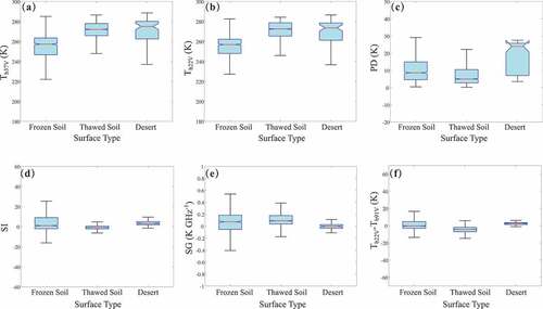
First, we analyzed and compared the distributions of the six spectral classification indices for three different ground types, frozen soil, thawed soil, and desert, based on all sample data from 2009 to demonstrate the differential spectral characteristics among the different ground types. The sample size of frozen soil was 212,946, the sample size of thawed soil was 642,590, and the sample size of the desert was 19,734. As shown in Figure 3, all of the three ground types exhibited different patterns in the six spectral classification indices. Specifically, the frozen ground had the lowest median values for T_b37V, while the desert had the highest values for T_b37V (Figure 3a). This indicates that T_b37V can serve as a good indicator to distinguish between frozen soil and deserts. Similarly, frozen ground and desert show different values of T_b22V (Figure 3b); however, T_b22V values of thawed ground are similar to those of desert, making it difficult to distinguish between thawed ground and desert in terms of the T_b22V values (Figure 3b). In terms of PD, the median PD value of the desert is approximately 25, which is the highest among the three ground types owing to its relatively smooth surface (Figure 3c). In contrast, the thawed ground had the lowest PD (Figure 3c). Moreover, the three ground types clearly demonstrate differences in SI with higher values for frozen soil and desert, indicating that they are strong scatterers and negative median values for thawed soil (Figure 3d). In addition, the three ground types also show different median values in SG, with negative values for desert and positive values for frozen ground and thawed ground. In contrast, the SG values of frozen soil are generally lower than those of thawed soil (Figure 3e). With regard to T_b22V-T_b91V, three ground types also showed different patterns (Figure 3f): values for thawed soil were negative, while median values for frozen ground were around 0 and desert were positive. Moreover, most of the notches in the box plot do not overlap with 95% confidence, so the true median is different for them. Overall, T_b37V and T_b22V were good indicators for distinguishing between thawed soil and frozen soil, while the other four indices showed marked differences among the three ground types (Figure 3). These results confirm that the six classification indices selected in this study can serve as good indicators for distinguishing the three ground types.

Figure 3. Comparison of six spectral classification indices of frozen soil, thawed soil, and desert: (a) T_b37V, (b) T_b22V, (c) PD, (d) SI, (e) SG, and (f) T_b22V-T_b91V.

3.2 Prediction accuracy assessment

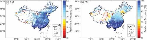
In the training phase, the validated prediction accuracy of the proposed FT-DESA was 92.85%. We further tested the FT-DESA results using the observations of all 2398 stations from 2010 to 2016 to assess their prediction efficiency. As described in Section 2.2.3, prediction accuracy was calculated at each station to measure the percentage of correctly predicted days to the total number of days. As a result, Figure 4 shows the spatial patterns of the prediction accuracy resulting from the AM and PM overpass data for all 2398 stations in 2011. The mean annual FT spatial prediction accuracy in relation to 2398 stations for 2011 is 89.4 ± 10.8% and 83.5 ± 16.8% for the AM and PM overpasses, respectively (Figure 4). The large standard deviation may relate to the relatively large accuracy difference between the southeast regions and the Tibetan Plateaus. The prediction accuracies in the southeast are mainly close to 100%, while the accuracies of some stations on the Tibetan Plateau are lower than 80%. The FT-DESA results based on the AM overpass observations have higher accuracy than those based on PM overpass observations, especially in the middle and high latitudes (Figure 4). In addition, the FT-DESA results have very high accuracy at lower latitudes because these regions are characterized by warmer climates and longer non-frozen periods (Figure 4). The above findings are consistent with SMAP (Xu et al. 2018) and AMSR2 (Wang et al. 2019a) FT products. However, one can note that the FT-DESA results have relatively lower accuracy than the observations in some desert/Gobi regions and parts of the Tibetan Plateau, especially for the PM results (Figure 4b). These results imply that the microwave spectral characteristics of deserts are essentially very close to those of some frozen ground, making it difficult for the algorithms to distinguish them completely.

Figure 4. Spatial distributions of the FT prediction accuracy (%) for the (a) AM and (b) PM overpasses in 2011.

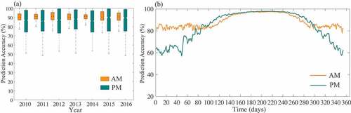
The prediction accuracy of each station from 2010 to 2016 and the mean prediction accuracy of daily FT-DESA classifications were also analyzed. As shown in Fig. 5a, the median prediction accuracy of the AM results was approximately 90% every year between 2010 and 2016, whereas the prediction accuracy of the PM results was approximately 86%. In addition, the prediction accuracy of the PM results has a wider spread than that of the AM results (Fig. 5a). The overall high accuracy for the AM and PM overpasses indicates that the developed FT-DESA algorithm has an overall good performance. Fig. 5b shows the mean prediction accuracy of the daily FT-DESA classifications for the AM and PM overpasses. The daily pattern for the PM overpass FT results indicates a higher accuracy in summer than in winter (Fig. 5b). In contrast, the daily accuracy for the AM overpass results is more consistent throughout the year. Again, the prediction accuracy of the PM results was generally lower than that of the AM (Figure 5b).

Figure 5. (a) Box plot of the FT prediction accuracy for the AM and PM overpasses from 2010 to 2016 and (b) mean prediction accuracy of daily FT-DESA classifications for the AM and PM overpasses.

3.3 Spatial patterns of the derived yearly FT cycle

We then used our trained FT-DESA algorithm to derive the FT status across China from 2009 to 2020 and further analyzed the spatiotemporal patterns of the derived FT cycles. Figure 6 shows the surface FT status on five dates on behalf of seasonal variability, in 2011. As shown in Figure 6a, the frozen area in China is the largest in winter, as defined by the FT image on 31 January 2011. In spring, represented by the FT image on 30 March 2011, the frozen area had largely shrunk (Figure 6b) because the air temperature was largely increased relative to winter. Some areas of the Tibetan Plateau and northeastern China, located in relatively cold regions, also showed thawed states on 30 March 2011. On 30 June 2011, most of China, except for a small portion of the Tibetan Plateau, and a few other small regions, showed thawed states (Figure 6c). On 30 September 2011, the thawed area and frozen areas started to decrease and increase, respectively, relative to the FT state on 30 June 2011 (Figure 6d). The frozen ground was mainly centered on the Tibetan Plateau and northeastern China (Figure 6d). On 31 December 2011, most of China showed a state of the frozen surface, except in the southern part of China, which belongs to non-frozen areas (Figure 6e and Figure 1).

Figure 6. Spatial distributions of the surface FT state retrieved by the FT-DESA on the representative days in 2011 represent the seasonality.

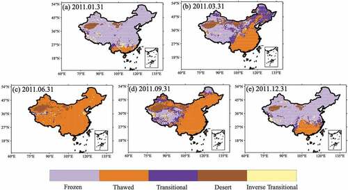
In terms of intra-day FT dynamics, areas that were frozen in the morning and thawed in the afternoon (i.e. the transitional state) were larger than those that were thawed in the morning and frozen in the afternoon (i.e. the inverse transitional state) (Figure 6). In addition, it is clear that the transitional FT state mostly occurred in northeast China and the Tibetan Plateau (e.g. Figures 6b,d). It is worth noting that some areas on the western edge of the Tibetan Plateau had inverse transitional FT states, which may be due to the complex changes in temperature on the Tibetan Plateau. Moreover, there may be some misclassifications owing to the disturbance of glaciers and lakes (Kim et al. 2017). Deserts, especially when covered by snow, also exhibit scattering characteristics similar to frozen surfaces and may be misclassified as frozen soil.

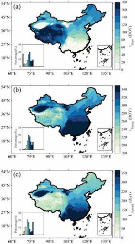
Three FT cycle metrics (t_thaw, t_freeze, and L_thawed) were obtained based on the classification results. As shown in Figure 7, the spatial patterns of the three FT cycle metrics are highly correlated with the map of permafrost types in China (Figure 1). Our results show that southeastern China, covering approximately 15% of the country, is a non-frozen area with t_thaw = 0, t_freeze = 365, and L_thawed = 365 (Figures 7a-c). The retrieved desert regions were mainly located around the northern part of the Tibetan Plateau, with no FT transitions (Figures 7a-c). The t_thaw occurred later in the Tibetan Plateau and northeastern China relative to the other regions (Figure 7a). In contrast, t_freeze occurred earlier in the same regions (Figure 7b) with a long frozen period (Figure 7c). The FT cycle exists in most areas of the Tibetan Plateau, including the ground active surface layer of the discontinuous permafrost regions. In contrast, t_thaw begins longer than the 180th day in the part of discontinuous permafrost regions. It should also be noted that the northern corner of Northeast China has a shorter thawing period than its surrounding area, as indicated by a later t_thaw (Figure 7a), an earlier t_freeze (Figure 7b), and a shorter L_thawed (Figure 7c). These results are in line with the spatial distribution of discontinuous permafrost in northeast China, as shown in Figure 1. Moreover, most of eastern and east-central China belongs to seasonally frozen areas (approximately 85% of China). Generally, the timing of the surface soil FT dynamics varies largely across China, which largely depends on the altitude and latitude (Figure 7). Primary landscape freezing usually occurs between September and November (Figure 7a), whereas primary landscape thawing normally occurs between March and May (Figure 7b). In parts of the western edge and central region of the Tibetan Plateau, some grid cells may be misclassified due to the impacts of glaciers and lakes (Figure 7) (Kim et al. 2017).

Figure 7. Spatial patterns of mean annual (a) t_freeze, (b) t_thaw, and (c) L_thawed from 2009 to 2020 based on the FT-DESA retrieval.

3.4 Evaluation of the FT cycle metrics and their spatial patterns from four FT products

To further verify the prediction accuracy of our proposed FT-DESA, we compared its results with those of three other FT algorithms. The three annual FT cycle metrics (t_thaw, t_freeze and L_thawed) derived from site observations and four FT retrieval algorithms (e.g. FT-DESA, MSTA, DTA, and DIA) were compared at the site scale. Because the original DTA and DIA algorithms retrieved the surface status using descending overpass data, we only compared the descending (AM) overpass results of the FT-DESA and MSTA algorithms with the DTA, DIA, and observations. The daily 0 cm soil temperatures of the China meteorological stations during the same period were used for validation as the real surface FT state.

Figure 8 shows the spatial distributions of mean annual t_thaw, t_freeze, and L_thawed from 2009 to 2015 for observations and the PM overpass results of the four FT algorithms. Overall, the spatial patterns of the t_thaw results of the four FT algorithms are generally consistent with the site observations (Figures 8a-e). However, the FT-DESA results agree better with the observations (Figure 8b) than the other three algorithms (Figures 8c-e). MSTA, DTA, and DIA tend to underestimate t_thaw in part of North China and Northeastern China (Figures 8a-e). We calculated the biases of each algorithm based on site-by-site comparisons to quantitatively explore the differences among the four algorithms. Table 1 demonstrates the overall performance of the four algorithms in t_thaw, t_freeze and L_thawed of surface frozen status. The regional average biases of the FT-DESA, MSTA, DTA, and DIA t_thaw results are 3.86 ± 13.90, −5.21 ± 38.51, −25.62 ± 28.50, and −9.81 ± 32.34 days, respectively (Table 1). The biases of the FT-DESA t_thaw results are generally the smallest among the four FT algorithms followed by the MTA results (Figures 9a,b), while DTA and DIA have the largest biases in t_thaw (Figures 9c,d). The biases of the FT-DESA t_thaw results are within ±10 days at about 60.13% of the 2398 stations, indicating that the FT-DESA algorithm has high accuracy in capturing the primary spring thawing across China (Figure 9a). The biases of the MSTA, DTA, and DIA t_thaw results are within ±10 days at about 30.23% (Figure 9b), 31.23% (Figure 9c), and 30.19% (Figure 9d) of the 2398 stations, respectively. In particular, MSTA, DTA, and DIA have large positive biases in North China (Figures 9b-d), indicating that the MSTA, DTA, and DIA algorithms tend to underestimate t_thaw in North China.

Figure 8. Spatial distributions of mean annual (a-e) t_thaw, (f-j) t_freeze, and (k-o) L_thawed for observations and the PM overpass results of four FT algorithms: FT-DESA, MSTA, DTA, and DIA.

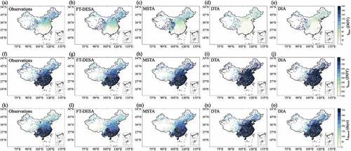
Figure 9. Spatial distributions of mean biases (retrieval-observation) of (a-d) t_thaw, (e-h) t_freeze, and (i-l) L_thawed for the PM overpass results of four FT algorithms: FT-DESA, MSTA, DTA, and DIA.

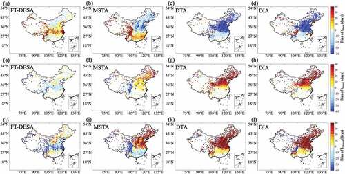
Table 1. Statistical metrics (bias and standard deviation (σ)) of the four algorithms in t_thaw, t_freeze and L_thawed of surface soil frozen status.

FT Index	FT-DESA	MSTA	DTA	DIA
	Bias\ σ (days)	Bias\ σ (days)	Bias\ σ (days)	Bias\ σ (days)
tthaw	3.86\13.9	5.21\38.51	−25.62\28.5	−9.81\32.34
tfreeze	−2.78\9.59	2.91\17.37	17.14\18.64	13.86\20.2
Lthawed	−6.64\23.51	8.12\44.28	42.77\43.12	23.67\49.57

The regional average biases of the FT-DESA, MSTA, DTA, and DIA t_freeze results are −2.78 ± 9.59, 2.91 ± 17.37, 17.14 ± 18.64, and 13.86 ± 20.20 days, respectively (Table 1). The biases of the FT-DESA t_freeze results are within ±10 days at approximately 73.69% of the 2398 stations. This shows that the t_freeze results of FT-DESA are generally consistent with the ground observations (Figure 9e). The biases of the MSTA, DTA, and DIA t_freeze results were within ±10 days at approximately 62.22% (Figure 9f), 50.17% (Figure 9g), and 44.62% (Figure 9h) of the 2398 stations, respectively. The bias of FT-DESA t_freeze is generally the lowest among the four FT algorithms, followed by MSTA results (Figures 9e,f), whereas DTA and DIA have the largest biases in t_freeze (Figures 9g,h). The significant positive biases are concentrated in the eastern region of the Tibetan Plateau in the MSTA algorithm. At the same time, DTA and DIA tend to overestimate t_freeze in North China (Figures 9g,h).

The regional average biases of the FT-DESA, MSTA, DTA, and DIA L_thawed results are −6.64 ± 23.51, 8.12 ± 44.28, 42.77 ± 43.12, and 23.67 ± 49.57 days, respectively (Table 1). The biases of the FT-DESA, MSTA, DTA, and DIA L_thawed results were within ±10 days at approximately 45.16% (Figure 9i), and 20.14% (Figure 9j), 28.98% (Figure 9k), and 25.73% (Figure 9l) of the 2398 stations, respectively. The FT-DESA algorithm tended to slightly overestimate t_thaw (Figure 9a) and underestimate t_freeze (Figure 9e), resulting in a slight underestimation in L_thawed (Figure 9i). However, the results of the other three FT algorithms are still the best. MSTA, DTA, and DIA tended to overestimate L_thawed in North China, with relatively large positive biases (Figures 9j-l). In addition, MSTA tends to underestimate L_thawed around the Tibetan Plateau (Figure 9j), which is consistent with the finding that the Tibetan Plateau is more unstable for MSTA during summer in the study by Wang et al. (2020).

Finally, we compared the mean annual FT cycle metrics for the four algorithms using box plots (Figure 10) and quantile-quantile plots (Figure 11) based on a site-by-site comparison. It is demonstrated that the FT-DESA algorithm has the lowest uncertainties and the narrowest error spreads in all three FT cycle metrics (Figures 10a-c). The MSTA algorithm has a generally higher uncertainty in the three FT cycle metrics than the FT-DESA algorithm (Figures 10a-c); however, the MSTA algorithm has lower uncertainties and narrower error spreads than the DTA and DIA algorithms (Figures 10a-c).

Figure 10. Box bars of biases (retrieval-observation) of (a) t_thaw, (b) t_freeze, (c) L_thawed for four FT algorithms.

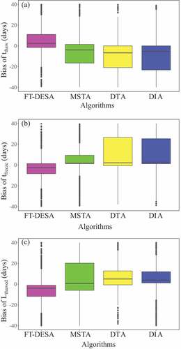
Figure 11. Quantile–quantile plots of the retrieved (a) t_thaw, (b) t_freeze, and (c) L_thawed by four FT algorithms vs. observations.

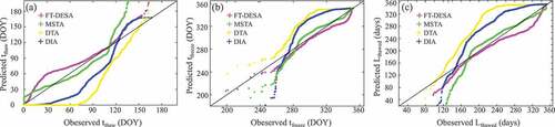
Moreover, one can also note that the quantile-quantile points of the FT-DESA results are generally closer to the one-to-one line than those of the other three algorithms. The distributions of biases are visible in the quantile-quantile plots. To facilitate the analysis of the results in Figure 11, we evenly divide the X-axis into three segments: early-t_thaw, intermediate-t_thaw and late-t_thaw section for t_thaw, early-t_freeze, intermediate-t_freeze and late-t_freeze section for t_freeze, short-L_thawed, intermediate-L_thawed and long-L_thawed section for L_thawed. The corresponding ranges were 0–60, 60–120, and 120–180 DOY for t_thaw. The corresponding ranges were 180–240, 240–300, and 300–360 DOY for t_freeze. The corresponding ranges were 0–120, 120–240, and 240–360 days for L_thawed. For example, FT-DESA tends to overestimate t_thaw when t_thaw falls between 20 and 60 days and when t_thaw is above 150 days; however, the FT-DESA results are close to the observations in the other ranges (Figure 11a). In contrast, MSTA tends to largely overestimate t_thaw when it is above 110 days and underestimate t_thaw when it is between 45 and 100 days (Figure 11a), although it is close to observations in the intermediate-t_thaw section. DTA and DIA mildly underestimate t_thaw when it is lower than 120 days (Figure 11a).

In terms of t_freeze and L_thawed, the quantile-quantile points of the FT-DESA results are the ones that are the closest to the one-by-one line (Figures 11b, c), although FT-DESA slightly underestimates t_freeze in the late-t_freeze section and underestimates L_thawed in the long-L_thawed section (Figures 11b, c). In contrast, DTA and DIA systematically overestimate t_freeze and L_thawed, while MSTA largely underestimates t_freeze in the early-t_freeze section and underestimates L_thawed in the short-L_thawed section (Figures 11b, c).

In general, the FT-DESA had the highest overall agreement with the observations, followed by MSTA and DIA (Figures 10 and 11). DTA had the largest errors among the four algorithms. The DTA significantly underestimated the freeze status and misclassified frozen soil as thawed soil at many stations.

4. Discussion

4.1 Advantages of the proposed algorithm

Using multifrequency brightness temperatures from SSMIS (2009–2020), we retrieved the surface FT states in China based on the freeze/thaw dynamic ensemble selection algorithm. This study adds new knowledge to FT retrieval algorithm development and can be distinguished from previous studies in three respects. First, we utilized daily dual-overpass (ascending and descending orbits), multi-bands, and dual-polarization T_b measurements from the SSMIS to classify daily FT dynamics. This allowed us to capture and consider intra-day FT dynamics and excludes the contaminations of deserts. Second, we adopted the dynamic ensemble selection model to dynamically integrate three machine learning models, namely, Random Forests, Extra-Trees, and Extreme Gradient Boosting, to optimally retrieve the surface FT states across China. The intercomparison between our developed FT retrieval algorithm and the other three existing algorithms has clearly demonstrated that our developed algorithm improved the FT retrieval accuracy. Finally, the samples used to train the FT-DESA to consider the characteristics of the major ground types and represent a wide range of elevations, illustrate that machine learning makes it possible to manage high-dimensional data and map features with complicated characteristics (Maxwell, Warner, and Fang 2018). In addition, we used an entire year of time series data to train the model, which can effectively reduce the impact of daily temperature fluctuations on FT retrieval. The modeling process is divided into training, validation, and testing phases, and the developed FT-DESA performs well in all three stages. The resultant trained algorithm had classification accuracies of approximately 88% and 84% for the AM and PM overpasses, respectively. The overall high accuracy for the AM and PM overpasses indicates that the developed FT-DESA algorithm has an overall good performance. Moreover, the FT-DESA algorithm has higher classification accuracy than the other three existing algorithms, proving the reliability and effectiveness of the proposed FT-DESA algorithm.

Moreover, three existing FT algorithms and FT-DESA are compared and verified by observed ground temperature. The validations indicate that some of the existing algorithms do not accurately reflect the temporal and spatial heterogeneity in selecting thresholds for FT classification and tend to overestimate or underestimate the timings of surface FT alternations. One should note that the FT data produced by the MSTA and DIA algorithms were directly taken from the existing products, which were calibrated with the training data likely different from those used in this study. This may introduce some uncertainty in the accuracy comparison. Nevertheless, we found that DTA and DIA estimate thaw earlier than observations at approximately 70% of the stations (Figures 9c,d). The underestimation of t_thaw in DTA and DIA may be related to the fact that the calibration of threshold values does not consider surface conditions (Shao and Zhang 2020). More specifically, DTA set the threshold of 37 GHz vertical polarization brightness temperature to 252 K based on soil temperature at 4 cm from only three stations that represent permafrost, seasonally frozen ground, and unfrozen regions in the Tibetan Plateau, respectively (Jin, Li, and Che 2009). Although the threshold value adopted by DTA conforms to the freeze/thaw boundary conditions in some regions, the annual average temperature of the Tibetan Plateau is low. The threshold condition is relatively high in humid regions, leading to a serious underestimation of soil freezing. Moreover, some studies have found that the thresholds in DIA and DTA could vary substantially in different regions and for different land cover types (Chang and Cao 1996; Roy et al. 2017a, 2017b; Zhang and Armstrong 2001). In contrast, MSTA uses the ERA-interim air temperature data to define the threshold for FT determination in each grid cell. According to a previous study (Shao and Zhang 2020), it performs better than DIA and DTA as a whole, suggesting that it was less impacted by climate type than DIA and DTA. Therefore, when these algorithms are used to retrieve surface soil FT dynamics, observation data should be selected to represent as many land types as possible. The threshold values of these algorithms should be calibrated for different land use and terrain types to improve the classification accuracy further. The primary spring thawing times detected by the MSTA product were generally earlier than the ground observations (Figure 9b and Figure 10a), while the primary fall freezing times detected by the MSTA product were overall later than the ground observations (Figure 9f and Figure 10b). The original MSTA product uses the ERA-interim reanalysis air temperature data rather than the observations to determine the threshold for the FT classification. Therefore, this may introduce some uncertainty in the resultant FT classifications (Wang et al. 2020). Overall, the reliability of our algorithm is proven by intercomparison analysis and provides a good reference on how well these four FT products are in the continuous and discontinuous permafrost and seasonally frozen ground regions of China.

4.2 Possible uncertainty sources and future works

We further investigated the potential sources of uncertainty and factors influencing the FT classification accuracy of our developed FT-DESA. One possible uncertainty may be the spatial interpolation of the brightness temperature data. To obtain spatiotemporally continuous brightness temperature, the brightness temperature data were interpolated using a sliding window method (Jin et al. 2015). For SSMIS brightness temperature data, global coverage can be completed approximately every 7 days. This interpolation method can achieve the spatiotemporal coverage of SSMIS brightness temperature data in China. However, changes in brightness temperature may be temporally significant and vary considerably in space, which may not be captured due to the data gaps and cannot be filled through the sliding window interpolation method. In addition, T_b can vary greatly because of the complex climate and surface conditions, especially during the FT diurnal variation, which can lead to certain errors during periods of sharp T_b fluctuations. However, a previous study proved that this interpolation method is generally effective and showed that the FT classification accuracy based on the interpolated data could remain close to the accuracy based on the original data in test areas (Shao 2021). Using site-level observations to compare with measurements over small regions/pixels by remote sensing instruments may also introduce uncertainty because of spatial heterogeneity in land cover types and topography. However, as the resolution of remote sensing imaging becomes finer, the uncertainty shall be lower (Chai et al. 2014). Our study also found that the FT classification accuracies of the existing algorithms were relatively low in arid areas, especially in the Tibetan Plateau (Figure 4), which is also common in the other FT algorithms (Wang et al. 2020). The FT dynamics on the Tibetan Plateau in the afternoon are much more complicated than in the morning during the seasonal cycle, making the accuracy of the PM overpass classification lower than that of the AM overpass classification daily (Fig. 5b). In addition, topography has a significant impact on passive microwave satellite signals over mountainous regions (Li et al. 2014). These conditions may cause a lower FT signal-to-noise ratio and lower prediction accuracy with observations (Grody and Basist 1996; Han et al. 2015). Moreover, Fig. 5b demonstrates that daily regional average prediction accuracy has the lowest and highest values during the winter-frozen season and summer non-frozen season, respectively. During the seasonal FT transition period and winter, the ice-water phase transformation process in near-surface soil generates a lot of latent heat. Repeated FT processes will occur in areas with severe daytime temperature fluctuations, leading to misclassification (Du et al. 2015; Kim et al. 2017).

On the other hand, there is a mismatch between the ascending local time and the time when the highest temperature of the day occurs, resulting in uncertainty in the FT retrieval in the ascending orbits. Considering that the soil temperature is generally stable between 0 am and 6 am (Fan, Liu, and Wang 2003), the descending local time of the SSMIS sensor (5 am) is highly aligned with the time when T_min appears. However, the ascending local time of the SMMIS sensor was approximately 17:31, which was generally later than the time when the daily maximum ground temperature appeared. This is believed to reduce the classification accuracy by weakening the relationship between T_g and T_b. Moreover, there is more FT variability over the intra-annual cycle in the PM record than in the AM record. The intra-day thawing may occur during the ascending orbit of the 0–1 cm soil depth, which has a substantial impact on detecting the FT states (Williamson et al. 2018). The varying range of the soil temperature measured in the decreasing orbit is relatively stable or small (Fan, Liu, and Wang 2003). Therefore, T_min is the optimal variable for calibrating and validating the algorithm (Jin et al. 2015). One of the core bases for distinguishing the freeze/thaw states is the change in the surface dielectric properties. Low soil moisture content in arid areas leads to insufficient water phase change in the processes of FT. As a result, the freezing factors used in the algorithm have no obvious seasonal variability (Wang et al. 2020). However, our developed FT-DESA algorithm generally performs well across the Tibetan Plateau based on the AM overpass data (Figure 4a). In addition, the classification accuracy can be further improved by a better desert masking because the desert may be covered with snow in a cold winter, which can affect the classification results.

It is worth noting that the thermometer measures the snow surface temperature instead of the soil temperature when the ground is covered by snow (Wang, Zhang, and Zhong 2015). This study assumes that the surface soil is frozen when covered by snow, because snow cover can only last when the surface soil temperature is below the freezing point (Zhang, Barry, and Armstrong 2003a). This assumption can be justified because previous studies have found that the classification accuracy during snow-covered periods is much better than that during snow-free periods (Zhang, Barry, and Armstrong 2003a). However, the presence of liquid water under snow produces dielectric properties similar to those under thawed conditions, which decreases the accuracy of detection (Shao and Zhang 2020). Snowmelt can also introduce some uncertainty in distinguishing the FT states in early spring. Nighttime data can be used to detect snow cover in mid-latitude mountains and polar regions (Huang et al. 2022), which may improve FT detection in the future.

Moreover, in this study, the 0 cm surface temperature reference datasets were used to evaluate the classification accuracies of the four freeze/thaw algorithms. Previous studies have used ground temperatures at different depths to validate the freeze/thaw algorithm. The mismatch between the depth of observation and the depth of passive microwave detection may also lead to a difference in the evaluation of FT indices. MSTA algorithm verified the results using air temperature data obtained from the National Climate Data Center Global Summary of the Day (Kim et al. 2017). The decision tree algorithm used 4 cm of ground temperature data from three observation stations in the Tibetan Plateau from CEOP to represent the real FT state of soil to verify the classifications (Jin, Li, and Che 2009). The dual-index algorithm adopted the daily minimum 0 cm surface temperatures from stations managed by the China Meteorological Administration for validation (Jin et al. 2015). Further research on the depth of passive microwave detection under different soil conditions will help establish the correlation between the confidence value and soil characteristics.

In addition, freezing point depression can affect the detection of the FT state (Pardo Lara et al. 2020). Substantial unfrozen water may also remain at temperatures well below zero due to hydrostatic pressure from capillary action in some soils (Painter and Karra 2014). However, there is currently no simple way to directly measure these phenomena and continuously for long-time and large-scale freeze/thaw retrieval, which should be considered in future studies on FT. Finally, although our developed FT-DESA algorithm based on three machine learning methods can generally capture the complex relationships among different ecohydrological processes to retrieve ground FT dynamics, it requires a large volume of data to train the model. In the future, it will be valuable to explore the effectiveness of this method when only limited in-situ data is available.

5. Conclusion

As a satellite-based FT retrieval algorithm, FT-DESA was developed to identify the surface soil FT state and consider the influences of the desert and intra-day FT dynamics. The mean classification accuracies of the model for the PM and AM overpasses were 89% and 84%, respectively. Moreover, we compared and evaluated our developed FT-DESA along with three other existing FT algorithms based on a site-by-site comparison. Our results show that the spatial distributions of the FT cycle metrics based on the FT-DESA record are the closest to the observations and that the biases in the FT-DESA results are also the lowest and narrowest among the four FT algorithms.

The validation and comparison results show that the FT-DESA by applying the KNORA-Union dynamic ensemble selection algorithm has produced a high-quality daily surface soil FT record from 2009 to 2020 using the SSMIS brightness temperature record. Daily FT records have reliably high accuracy and provide a trustworthy dataset to analyze the timing, duration, and spatial extent of surface soil FT dynamics. It can be used to retrieve the FT states in these regions without ground observations. It can also provide valuable information for studies on climate change, interactions on the cryosphere, hydrological processes, and carbon and energy cycles. We also argue that uncertainties and limitations still exist in detecting long-term surface soil FT status due to the impacts of terrain, soil texture, and freezing point depression among others. Therefore, it is necessary to optimize the algorithm in different areas further to enhance its sensitivity to temperature and soil moisture changes in the future.

Credit authorship contribution statement

Xi Li: Conceptualization; Data curation; Software; Methodology; Validation; Writing-original draft; Writing-review & editing. Ke Zhang: Conceptualization; Methodology; Writing-original draft; Writing-review & editing; Supervision; Resources; Funding acquisition. Jiefan Niu: Conceptualization. Linxin Liu: Data curation.

Acknowledgements

This study was supported by the National Natural Science Foundation of China (51879067), Fundamental Research Funds for the Central Universities of China (B220203051), and Hydraulic Science and Technology Plan Foundation of Shaanxi Province (2019slkj-B1).

Funding

This work was supported by the National Natural Science Foundation of China [51879067]; Fundamental Research Funds for the Central Universities [B200204038]; Hydraulic Science and Technology Plan Foundation of Shaanxi Province [2019slkj-B1].

Disclosure statement

No potential conflict of interest was reported by the author(s).

Data availability statement

The SSMIS brightness temperature data are available from the Remote Sensing Systems (http://www.remss.com/). The observed ground temperature is available from the Daily Data Set of Basic Meteorological Elements of National Surface Meteorological Stations in China (V3.0) (https://data.tpdc.ac.cn/). The land-use data are available from the Resource and Environment Science and Data Center (http://www.resdc.cn/). The permafrost map is available from the Resource and Environment Science and Data Center (http://www.resdc.cn/). The dual-index algorithm (DIA) (2009-2015) is released by National Tibetan Plateau Data Center (https://data.tpdc.ac.cn/). The modified seasonal threshold algorithm (MSTA) (2009-2015) is released by the American Snow and Ice Data Center (https://nsidc.org). The source code of the KNORA-UNION dynamic ensemble selection algorithm is available from https://github.com/scikit-learn-contrib/DESlib/tree/master/deslib/des/.

References

- Błaszczyk, M., and J. Jȩdrzejowicz. 2021. “Framework for Imbalanced Data Classification.” Procedia Computer Science 192: 3477–3486. doi:10.1016/j.procs.2021.09.121.
- Bommarito, J. 1993. “Dmsp Special Sensor Microwave Imager Sounder (SSMIS).” Microwave Instrumentation for Remote Sensing of the Earth 1935: 230–238.
- Britto, A. S., Jr, R. Sabourin, and L. E. Oliveira. 2014. “Dynamic Selection of classifiers—a Comprehensive Review.”Pattern Recognition 47 (11): 3665–3680 10.1016/j.patcog.2014.05.003
- Chai, L. N., L. X. Zhang, Y. Y. Zhang, Z. G. Hao, L. M. Jiang, and S. J. Zhao. 2014. “Comparison of the Classification Accuracy of Three Soil freeze-thaw Discrimination Algorithms in China Using SSMIS and AMSR-E Passive Microwave Imagery.” International Journal of Remote Sensing 35 (22): 7631–7649. doi:10.1080/01431161.2014.975376.
- Chang, A. T. C., and M. S. Cao. 1996. “Monitoring Soil Condition in the Northern Tibetan Plateau Using SSM/I Data.” Nordic Hydrology 27 (3): 175–184. doi:10.2166/nh.1996.0003.
- Cruz, R. M., L. G. Hafemann, R. Sabourin, and G. D. Cavalcanti. 2020. “DESlib: A Dynamic Ensemble Selection Library in Python.” Journal of Machine Learning Research: JMLR 21 (79): 1–5.
- Cruz, R. M. O., D. V. R. Oliveira, G. D. C. Cavalcanti, and R. Sabourin. 2019. “FIRE-DES Plus Plus: Enhanced Online Pruning of Base Classifiers for Dynamic Ensemble Selection.” Pattern Recognition 85: 149–160. doi:10.1016/j.patcog.2018.07.037.
- Cruz, R. M. O., R. Sabourin, and G. D. C. Cavalcanti. 2018. “Dynamic Classifier Selection: Recent Advances and Perspectives.” Information Fusion 41: 195–216. doi:10.1016/j.inffus.2017.09.010.
- Dietterich, T. G. 2000. “Ensemble Methods in Machine Learning.” Multiple Classifier Systems 1857: 1–15.
- Dogo, E. M., N. I. Nwulu, B. Twala, and C. Aigbavboa. 2021. “Accessing Imbalance Learning Using Dynamic Selection Approach in Water Quality Anomaly Detection.” Symmetry 13 (5): 818. doi:10.3390/sym13050818.
- Dos Santos, E. M., R. Sabourin, and P. Maupin. 2008. “A Dynamic overproduce-and-choose Strategy for the Selection of Classifier Ensembles.” Pattern Recognition 41 (10): 2993–3009. doi:10.1016/j.patcog.2008.03.027.
- Du, J. Y., J. S. Kimball, M. Azarderakhsh, R. S. Dunbar, M. Moghaddam, and K. C. McDonald. 2015. “Classification of Alaska Spring Thaw Characteristics Using Satellite L-Band Radar Remote Sensing.” Ieee Transactions on Geoscience and Remote Sensing 53 (1): 542–556. doi:10.1109/TGRS.2014.2325409.
- England, A. W., J. F. Galantowicz, and B. W. Zuerndorfer. 1991. “A Volume Scattering Explanation for the Negative Spectral Gradient of Frozen Soil.” Igarss 91 - Remote Sensing: Global Monitoring for Earth Management 1-4: 1175–1177.
- Fan, A. W., W. Liu, and C. Q. Wang. 2003. Numerical Simulation of Diurnal Variation of Soil Temperature under Different Environmental Conditions. Acta Solar Energy 02: 167–171(In. Chinese
- Fausett, L. V. 2006. Fundamentals of Neural Networks: Architectures, Algorithms and Applications. Chennai, India: Pearson Education India.
- Fernández-Delgado, M., E. Cernadas, S. Barro, and D. Amorim. 2014. “Do We Need Hundreds of Classifiers to Solve Real World Classification Problems?” The Journal of Machine Learning Research 15: 3133–3181.
- Frolking, S., K. C. McDonald, J. S. Kimball, J. B. Way, R. Zimmermann, and S. W. Running. 1999. “Using the space-borne NASA Scatterometer (NSCAT) to Determine the Frozen and Thawed Seasons.” Journal of Geophysical Research-Atmospheres 104 (D22): 27895–27907. doi:10.1029/1998JD200093.
- Grody, N. C., and A. N. Basist. 1996. “Global Identification of Snowcover Using SSM/I Measurements.” Ieee Transactions on Geoscience and Remote Sensing 34 (1): 237–249. doi:10.1109/36.481908.
- Han, M. L., K. Yang, J. Qin, R. Jin, Y. M. Ma, J. Wen, Y. Y. Chen, L. Zhao, L. Zhu, and W. J. Tang. 2015. “An Algorithm Based on the Standard Deviation of Passive Microwave Brightness Temperatures for Monitoring Soil Surface freeze/thaw State on the Tibetan Plateau.” Ieee Transactions on Geoscience and Remote Sensing 53 (5): 2775–2783. doi:10.1109/TGRS.2014.2364823.
- Huang, Y., Z. C. Song, H. X. Yang, B. L. Yu, H. X. Liu, T. Che, J. Chen, J. P. Wu, S. Shu, and X. B. Peng. 2022. “Snow Cover Detection in mid-latitude Mountainous and Polar Regions Using Nighttime Light Data.” Remote Sensing of Environment 268: 112766. doi:10.1016/j.rse.2021.112766.
- Hu, T. X., T. J. Zhao, J. C. Shi, S. L. Wu, D. Liu, H. M. Qin, and K. G. Zhao. 2017. “High-resolution Mapping of freeze/thaw Status in China via Fusion of MODIS and AMSR2 Data.” Remote Sensing 9 (12): 1339. doi:10.3390/rs9121339.
- Jin, R. 2016. Long-term Land Surface freeze/thaw Status Datasets of China. Remote Sensing Technology and Application 31: 820–826(In. Chinese
- Jin, R., X. Li, and T. Che. 2009. “A Decision Tree Algorithm for Surface Soil freeze/thaw Classification over China Using SSM/I Brightness Temperature.” Remote Sensing of Environment 113 (12): 2651–2660. doi:10.1016/j.rse.2009.08.003.
- Jin, R., T. J. Zhang, X. Li, X. G. Yang, and Y. H. Ran. 2015. “Mapping Surface Soil freeze-thaw Cycles in China Based on SMMR and SSM/I Brightness Temperatures from 1978 to 2008.” Arctic Antarctic and Alpine Research 47 (2): 213–229. doi:10.1657/AAAR00C-13-304.
- Kim, Y., J. S. Kimball, J. Glassy, and J. Du. 2017. “An Extended Global Earth System Data Record on Daily Landscape freeze-thaw Determined from Satellite Passive Microwave Remote Sensing.” Earth System Science Data 9 (1): 133–147. doi:10.5194/essd-9-133-2017.
- Kim, Y., J. S. Kimball, K. C. McDonald, and J. Glassy. 2011. “Developing a Global Data Record of Daily Landscape Freeze/Thaw Status Using Satellite Passive Microwave Remote Sensing.” Ieee Transactions on Geoscience and Remote Sensing 49 (3): 949–960. doi:10.1109/TGRS.2010.2070515.
- Kim, Y., J. S. Kimball, K. Zhang, and K. C. McDonald. 2012. “Satellite Detection of Increasing Northern Hemisphere non-frozen Seasons from 1979 to 2008: Implications for Regional Vegetation Growth.” Remote Sensing of Environment 121: 472–487. doi:10.1016/j.rse.2012.02.014.
- Ko, A. H. R., R. Sabourin, and A. S. Britto. 2008. “From Dynamic Classifier Selection to Dynamic Ensemble Selection.” Pattern Recognition 41 (5): 1718–1731. doi:10.1016/j.patcog.2007.10.015.
- Kuncheva, L. I., and J. J. Rodriguez. 2007. “Classifier Ensembles with a Random Linear Oracle.” IEEE Transactions on Knowledge and Data Engineering 19 (4): 500–508. doi:10.1109/TKDE.2007.1016.
- Li, X. J., Y. J. Li, and X. X. Zhu. 2007. Identification of Snow Cover in China and Its Surrounding Areas Using SSM/I Data. Journal of Applied Meteorological Science 01: 12–20. In Chinese
- Li, X., Z. T. Nan, and Y. W. Zhou. 2012. Map of 1:10000 000 Permafrost Types in China (2008). Beijing: C. National Tibetan Plateau Data (Ed.): National Tibetan Plateau Data Center.
- Li, X. X., L. X. Zhang, L. Weihermuller, L. M. Jiang, and H. Vereecken. 2014. “Measurement and Simulation of Topographic Effects on Passive Microwave Remote Sensing over Mountain Areas: A Case Study from the Tibetan Plateau.” Ieee Transactions on Geoscience and Remote Sensing 52 (2): 1489–1501. doi:10.1109/TGRS.2013.2251887.
- Maxwell, A. E., T. A. Warner, and F. Fang. 2018. “Implementation of machine-learning Classification in Remote Sensing: An Applied Review.” International Journal of Remote Sensing 39 (9): 2784–2817. doi:10.1080/01431161.2018.1433343.
- McFarland, M. J., R. L. Miller, and C. M. Neale. 1990. “Land Surface Temperature Derived from the SSM/I Passive Microwave Brightness Temperatures.” Ieee Transactions on Geoscience and Remote Sensing 28 (5): 839–845. doi:10.1109/36.58971.
- Merchant, M. A., M. Obadia, B. Brisco, B. DeVries, and A. Berg. 2022. “Applying Machine Learning and Time-Series Analysis on Sentinel-1A SAR/InSAR for Characterizing Arctic Tundra Hydro-Ecological Conditions.” Remote Sensing 14 (5): 1123. doi:10.3390/rs14051123.
- National Meteorological Information, C. 2019. Daily Meteorological Dataset of Basic Meteorological Elements of China National Surface Weather Station (V3.0) (1951-2010). Beijing: C. National Tibetan Plateau Data (Ed.): National Tibetan Plateau Data Center.
- National Tibetan Plateau Data Center. 2019. Landuse Dataset in China (1980-2015), edited by National Science & Technology Infrastructure.
- Painter, S. L., and S. Karra. 2014. “Constitutive Model for Unfrozen Water Content in Subfreezing Unsaturated Soils.” Vadose Zone Journal 13 (4): 1–8. doi:10.2136/vzj2013.04.0071.
- Pardo Lara, R., A. A. Berg, J. Warland, and G. Parkin. 2021. “Implications of Measurement Metrics on Soil Freezing Curves: A Simulation of freeze–thaw Hysteresis.” Hydrological Processes 35 (7): e14269. doi:10.1002/hyp.14269.
- Pardo Lara, R., A. Berg, J. Warland, and E. Tetlock. 2020. “In Situ Estimates of freezing/melting Point Depression in Agricultural Soils Using Permittivity and Temperature Measurements.” Water Resources Research 56 (5): e2019WR026020. doi:10.1029/2019WR026020.
- Rautiainen, K., J. Lemmetyinen, M. Schwank, A. Kontu, C. B. Menard, C. Matzler, M. Drusch, A. Wiesmann, J. Ikonen, and J. Pulliainen. 2014. “Detection of Soil Freezing from L-band Passive Microwave Observations.” Remote Sensing of Environment 147: 206–218. doi:10.1016/j.rse.2014.03.007.
- Rautiainen, K., T. Parkkinen, J. Lemmetyinen, M. Schwank, A. Wiesmann, J. Ikonen, C. Derksen, et al. 2016. “SMOS Prototype Algorithm for Detecting Autumn Soil Freezing.” Remote Sensing of Environment 180: 346–360. doi:10.1016/j.rse.2016.01.012.
- Renner, R. S. (2000). Systems of Ensemble Networks Demonstrate Superiority over Individual Cascor Nets. Ic-Ai’2000: Proceedings of the International Conference on Artificial Intelligence, Las Vegas, Nevada, USA, Vol 1-Iii, 367–373
- Roy, A., A. Royer, C. Derksen, L. Brucker, A. Langlois, A. Mialon, and Y. H. Kerr. 2015. “Evaluation of Spaceborne L-Band Radiometer Measurements for Terrestrial freeze/thaw Retrievals in Canada.” Ieee Journal of Selected Topics in Applied Earth Observations and Remote Sensing 8 (9): 4442–4459. doi:10.1109/JSTARS.2015.2476358.
- Roy, A., P. Toose, C. Derksen, T. Rowlandson, A. Berg, J. Lemmetyinen, A. Royer, E. Tetlock, W. Helgason, and O. Sonnentag. 2017a. “Spatial Variability of L-band Brightness Temperature during freeze/thaw Events over a Prairie Environment.” Remote Sensing 9 (9): 894. doi:10.3390/rs9090894.
- Roy, A., P. Toose, M. Williamson, T. Rowlandson, C. Derksen, A. Royer, A. A. Berg, J. Lemmetyinen, and L. Arnold. 2017b. “Response of L-Band Brightness Temperatures to freeze/thaw and Snow Dynamics in a Prairie Environment from ground-based Radiometer Measurements.” Remote Sensing of Environment 191: 67–80. doi:10.1016/j.rse.2017.01.017.
- Schuur, E. A. G., B. Abbott, and P. C. Network. 2011. “High Risk of Permafrost Thaw.” Nature 480 (7375): 32–33. doi:10.1038/480032a.
- Shao, W. W. 2021. Monitoring high-resolution Soil freezing-thawing Changes Using Passive Microwave Remote Sensing in the Northern Hemisphere. Lanzhou: Lanzhou University.
- Shao, W. W., and T. J. Zhang. 2020. “Assessment of Four near-surface Soil freeze/thaw Detection Algorithms Based on Calibrated Passive Microwave Remote Sensing Data over China.” Earth and Space Science 7 (7): e2019EA000807. doi:10.1029/2019EA000807.
- Shirmard, H., E. Farahbakhsh, R. D. Müller, and R. Chandra. 2022. “A Review of Machine Learning in Processing Remote Sensing Data for Mineral Exploration.” Remote Sensing of Environment 268: 112750. doi:10.1016/j.rse.2021.112750.
- Wang, J., L. M. Jiang, H. Z. Cui, G. X. Wang, J. W. Yang, X. J. Liu, and X. Su. 2020. “Evaluation and Analysis of SMAP, AMSR2 and MEaSUREs freeze/thaw Products in China.” Remote Sensing of Environment 242: 111734. doi:10.1016/j.rse.2020.111734.
- Wang, J. Y., C. C. Song, A. X. Hou, and F. M. Xi. 2017. “Methane Emission Potential from Freshwater Marsh Soils of Northeast China: Response to Simulated freezing-thawing Cycles.” Wetlands 37 (3): 437–445. doi:10.1007/s13157-017-0879-3.
- Wang, Q. Q., K. Zhang, J. Y. Ye, and Z. J. Li. 2019b. Spatial-temporal Variation of Soil Moisture and Remote Sensing Inversion in Anhui Province. Journal of Hohai University 47: 114–118. (In Chinese)
- Wang, K., T. Zhang, and X. Zhong. 2015. “Changes in the Timing and Duration of the near-surface Soil freeze/thaw Status from 1956 to 2006 across China.” Cryosphere 9 (3): 1321–1331. doi:10.5194/tc-9-1321-2015.
- Wang, P. K., T. J. Zhao, J. C. Shi, T. X. Hu, A. Roy, Y. B. Qiu, and H. Lu. 2019a. “Parameterization of the freeze/thaw Discriminant Function Algorithm Using Dense in-situ Observation Network Data.” International Journal of Digital Earth 12 (8): 980–994. doi:10.1080/17538947.2018.1452300.
- Williamson, M., T. L. Rowlandson, A. A. Berg, A. Roy, P. Toose, C. Derksen, L. Arnold, and E. Tetlock. 2018. “L-band Radiometry freeze/thaw Validation Using Air Temperature and Ground Measurements.” Remote Sensing Letters 9 (4): 403–410. doi:10.1080/2150704X.2017.1422872.
- Xie, Y., R. Jin, and X. G. Yang. 2013. “Algorithm Development of Monitoring Daily near Surface freeze/thaw Cycles Using AMSR-E Brightness Temperature.” Remote Sensing Technology and Application 28 (2): 182–191.
- Xu, X., R. S. Dunbar, C. Derksen, A. Colliander, Y. Kim, and J. S. Kimball. 2018. SMAP L3 Radiometer Global and Northern Hemisphere Daily 36 Km EASE-grid freeze/thaw State. version 2. Boulder, Colorado, USA: NASA National Snow and Ice datacenter.
- Ye, R., and Q. Dai. 2018. “A Novel Greedy Randomized Dynamic Ensemble Selection Algorithm.” Neural Processing Letters 47: 565–599.
- Zhang, T., and R. L. Armstrong. 2001. “Soil freeze/thaw Cycles over snow-free Land Detected by Passive Microwave Remote Sensing.” Geophysical Research Letters 28 (5): 763–766. doi:10.1029/2000GL011952.
- Zhang, T., R. L. Armstrong, and J. Smith. 2003b. “Investigation of the near-surface Soil freeze-thaw Cycle in the Contiguous United States: Algorithm Development and Validation.” Journal of Geophysical Research: Atmospheres 108 (D22). doi:10.1029/2003JD003530.
- Zhang, T., R. G. Barry, and R. L. Armstrong. 2004. “Application of Satellite Remote Sensing Techniques to Frozen Ground Studies.” Polar Geography 28 (3): 163–196. doi:10.1080/789610186.
- Zhang, K., L. J. Chao, Q. Q. Wang, Y. C. Huang, R. H. Liu, Y. Hong, Y. Tu, W. Qu, and J. Y. Ye. 2019. “Using multi-satellite Microwave Remote Sensing Observations for Retrieval of Daily Surface Soil Moisture across China.” Water Science and Engineering 12 (2): 85–97. doi:10.1016/j.wse.2019.06.001.
- Zhang, K., J. F. Niu, X. Li, and L. J. Chao. 2021. Comparison of Application of Intelligent Flood Forecasting Model in semi-arid and semi-humid Region of China. Water Resources Protection 201: 28–35(In. Chinese
- Zhang, L. X., J. C. Shi, Z. J. Zhang, and K. G. Zhao (2003a). The Estimation of Dielectric Constant of Frozen soil-water Mixture at Microwave Bands. Igarss 2003: Ieee International Geoscience and Remote Sensing Symposium, Vols I - Vii, Proceedings Toulouse, 2903–2905
- Zhao, T. J., L. X. Zhang, L. M. Jiang, S. J. Zhao, L. N. Chai, and R. Jin. 2011. “A New Soil freeze/thaw Discriminant Algorithm Using AMSR-E Passive Microwave Imagery.” Hydrological Processes 25 (11): 1704–1716. doi:10.1002/hyp.7930.
- Zhao, L., D. F. Zou, G. J. Hu, T. H. Wu, E. J. Du, G. Y. Liu, Y. Xiao, et al. 2021. “A Synthesis Dataset of Permafrost Thermal State for the Qinghai-Tibet (Xizang) Plateau, China.” Earth System Science Data 13 (8): 4207–4218. doi:10.5194/essd-13-4207-2021.
- Zheng, G. H., Y. T. Yang, D. W. Yang, B. Dafflon, Y. H. Yi, S. L. Zhang, D. L. Chen, et al. 2020. “Remote Sensing Spatiotemporal Patterns of Frozen Soil and the Environmental Controls over the Tibetan Plateau during 2002-2016.” Remote Sensing of Environment 247: 111927. doi:10.1016/j.rse.2020.111927.
- Zhu, X. 2019. Research on Dynamic Ensemble Classification Method. Dalian: Dalian Maritime University.
- Zuerndorfer, B., and A. W. England. 1992. “Radiobrightness Decision Criteria for freeze/thaw Boundaries.” Ieee Transactions on Geoscience and Remote Sensing 30 (1): 89–102. doi:10.1109/36.124219.
- Zwieback, S., C. Paulik, and W. Wagner. 2015. “Frozen Soil Detection Based on Advanced Scatterometer Observations and Air Temperature Data as Part of Soil Moisture Retrieval.” Remote Sensing 7 (3): 3206–3231. doi:10.3390/rs70303206.