Modeling of spatial stratified heterogeneity

ABSTRACT

Spatial stratified heterogeneity (SSH) refers to the geographical phenomena in which the geographical attributes within-strata are more similar than the between-strata, which is ubiquitous in the real world and offers information implying the causation of nature. Stratification, a primary approach to SSH, generates strata using a priori knowledge or thousands of supervised and unsupervised learning methods. Selecting reasonable stratification methods for spatial analysis in specific domains without prior knowledge is challenging because no method is optimal in a general sense. However, a systematic review of a large number of stratification methods is still lacking. In this article, we review the methods for stratification, categorize the existing typical stratification methods into four classes – univariate stratification, cluster-based stratification, multicriteria stratification, and supervised stratification – and construct their taxonomy. Finally, we present a summary of the software and tools used to compare and perform stratification methods. Given that different stratification methods reflect distinct human understandings of spatial distributions and associations, we suggest that further studies are needed to reveal the nature of geographical attributes by integrating SSH, advanced algorithms, and interdisciplinary methods.

KEYWORDS:

• Spatial stratified heterogeneity
• stratification
• cluster analysis
• spatial statistics
• geographical detector

1. Introduction

Spatial heterogeneity (SH) is of great importance in the study of earth science, ecology, and public health. SH is defined either as the variation in space in the distribution of a point pattern or as the variation in the qualitative or quantitative value of a surface pattern (Dutilleul and Legendre 1993). Spatial heterogeneity disrupts the stationarity assumptions underpinning many spatial models (Gaetan and Guyon 2010); therefore, it is crucial to summarize the models used to deal with spatial heterogeneity. On a spatial scale, SH can be classified as spatial local heterogeneity (SLH) or spatial stratified heterogeneity (SSH) (Wang, Zhang, and Fu 2016). SLH explores the local spatial cluster with similarity in geographical attributes. For instance, there are many indicators to detect hot spots, such as local indicators of spatial association (LISA) (Anselin 1995), Getis–Ord Gi (Getis and Ord 1992), spatial scan statistics (Kulldorff 1997), and for processing spatial local effects by geographically weighted regression (GWR) and its extended models (Brunsdon, Fotheringham, and Charlton 1998; Fotheringham, Yang, and Kang 2017; Huang, Wu, and Barry 2010).

SSH emphasizes the heterogeneity between strata, and each stratum is composed of a number of spatial objects. For study variables in different strata, the heterogeneity may exist in significantly different means and dominant factors, as well as various relationships with the explanatory variables. For example, precipitation has a dome-shaped effect on human plague in the north and a U-shaped effect in the south China (Xu et al. 2011), the human plague is spatial stratified heterogeneity on north and South China. Strata can be constructed through a stratification process based on prior knowledge or with the aid of quantitative methods, such as clustering analysis (Jain 2010; Jain, Murty, and Flynn 1999) and spatially constrained clustering (Lankford 2010; AssunÇão et al. 2006). The geographical detector model (Wang, Zhang, and Fu 2016; Wang et al. 2010) is a primary and popular tool for the SSH, widely used for measuring the SSH and evaluating the determinant power of potential explanatory variables (Yin et al. 2019; Hu et al. 2020; Xu et al. 2021). Other main models based on SSH are Sandwich (Wang et al. 2013), a mapping method for strong SSH, and the mean of the surface with non-homogeneity (MSN), which considers both spatial autocorrelation and SSH in mean estimation or spatial interpolation (Wang, Li, and Christakos 2009; Gao et al. 2020). Unlike the local model, model parameters based on SSH vary only across strata rather than varying with spatial location as in GWR. These models achieve a good trade-off between producing general results (i.e. model parameters do not vary with spatial location) and capturing local variations (i.e. parameters are allowed to vary across locations).

Stratification is one of the vital steps in research on SSH and is conducted mainly by the process based on prior knowledge (e.g. Kӧppen climate classification system (Köppen 1931) and ecoregions of the United States (Bailey 1995)) or a few quantitative methods, such as clustering analysis (Jain 2010; Jain, Murty, and Flynn 1999), spatially constrained clustering (Lankford 2010; AssunÇão et al. 2006), and regression tree (Breiman et al. 1984). In explaining spatial heterogeneity, stratification has advantages in four major aspects. First, stratification results (i.e. strata) are qualitative data, and learning from qualitative data is often more effective and more efficient than learning from quantitative data or data of a mixed type. Second, stratification converts continuous explanatory variables into strata to find complex nonlinear correlations with the study variable (Luo, Song, and Wu 2021; Xu et al. 2011). Third, stratification can identify confounding factors by replacing unobserved data with strata based on expert experience (Wu, Li, and Guo 2021). Finally, stratification has been proven to be an effective way to improve the accuracy of spatial sampling and inference using several models, such as stratified kriging (Stein, Hoogerwerf, and Bouma 1988; Weber and Englund 1992), geographical detector-based stratified regression kriging (Liu et al. 2021), and Biased Sample Hospital-based Area Disease Estimation (B-SHADE) (Wang et al. 2011; Xu, Wang, and Li 2018).

Although some studies have conducted stratification based on SSH (Cao, Ge, and Wang 2013; Song et al. 2020; Meng et al. 2021), the selection of stratification methods usually hinges upon individual preferences, which often leads to unconvincing results. Therefore, attention still needs to be paid to the differences between these stratification methods, and a more systematic study of stratification is urgently required for scientific instruction. The main contributions of this work are as follows:

Summarize the general criteria for stratification based on statistical characteristics of the data and study context

Construct the taxonomy of stratification algorithms according to the number of variables, exploratory or predictive task, and single or multiple criteria and the relationships among algorithms

Provide the guidelines for selection of stratification algorithms based on input parameters, robustness, arbitrary shape, and scalability to large data, and available software packages for stratification in R, Python, Geoda, ArcGIS, and QGIS

Discuss the assessment of results of stratification and future recommendations.

The remainder is organized as follows. Section 2 and Section 3 describe the definition, processing and criteria of stratification. Section 4 covers the main algorithms of stratification. Section 5 summarizes the stratification methods and gives common software packages for stratification. Sections 6 and 7 present the discussion and conclusions of the study, respectively.

2. Definition and processing of stratification

2.1. Definition

By “stratification,” we mean organizing geographical objects into subsets (called strata) based on the similarity of their attributes or spatial relationships. Stratification in spatial analysis is usually undertaken on a geographical basis, for example, by dividing the study area into subregions by variables, especially for the purpose of sampling (Cochran 1977) or statistical inference (Wang et al. 2013; Wang, Gao, and Stein 2020). There are many terms similar to stratification, such as “clustering,” “classification,” and “regionalization.” Although the three terms aim to group the study population into different subgroups, there are some minor differences among them. Clustering and regionalization always involve unlabeled data (unsupervised learning), and regionalization methods are also known as spatially constrained aggregation methods, zone design, and constrained clustering (Duque, Ramos, and Surinach 2007); while classification involves labeled data (supervised learning) (Duda, Hart, and Stork 2000). In regionalization, only adjacent zones may be merged to form regions, which is the distinction between regionalization and classification or clustering. In this paper, we refer to them collectively as “stratification” in the domains of SSH. Strata can be either attribute groups (result of clustering or classification) or spatially connected zones (result of regionalization).

2.2. Processing of stratification

Stratification processing consists of four steps, that is, selection of explanatory variables, determination of stratification criteria, stratification, assessment of result. Figure 1 depicts a typical sequencing of these steps.

Figure 1. The processing of stratification.

1. Selection of explanatory variables is to choose distinguishing features from a set of candidates according to the study variables. The explanatory variables may be nominal, ordinal, interval scaled, or of mixed types.

Determination of stratification criteria refers to the abstraction of the research problem based on the study task, classified as exploratory task and predictive task, the criteria of stratification, and stratification for each explanatory variable or all variables.

Stratification step is choosing the algorithm based on the pattern representation, the available software packages and the users’ understanding of algorithms.

Assessment of result can be performed by q-statistic for (Wang, Zhang, and Fu 2016; Wang et al. 2010). If the stratification result is too far from the expected one, we could reselect explanatory variables as well as the stratification algorithm.

The outputs of stratification need to be interpreted with experimental evidence and analysis, so that convincing conclusions could be drawn, and the strata can be used for sampling or modeling.

3. Stratification criteria

Stratification is often driven by the study task is exploratory or predictive, the number of variables, and criteria of the algorithm. The predictive task can be solved by supervised learning method and focuses on the performance on new variables data; while exploratory task is solved by unsupervised learning method and focuses on the patterns reflected by the current variables data. The number of variables of each stratification determines whether a univariate or multivariate approach is used. The criterion of the algorithm reflects our understanding of the problem and is the more central issue in the stratification. In this section, we focus only on several general and popular criteria, which are summarized below:

3.1. Homogeneity

Spatial objects in the same strata should be as similar as possible in terms of attributes relevant to the analysis. Similarity can be measured using within-strata variability, distance matrices, or probability models.

• (2) Within-strata variability. It measures the variation of objects to the representative points of each stratum. The search for strata of maximum homogeneity leads to minimum within-strata variability. Let be the set of $m$-dimensional points. The within-strata variability can be calculated as follows:

(1) $J(s)=\sum _{k=1}^k\sum _{x_i\in s_k}^{\hspace{0.17em}}||x_i-c_k|{|}^2$(1)

where $c_k$ is the representative point of stratum $k$. If $c_k$ is the mean value in stratum $k$, $J\left(s\right)$ is the objective function of the K-means (Ball and Hall 1965; MacQueen 1967) and Jenks natural breaks (JNB) (Fisher 1958; Jenks 1977). If $c_k$ is the medoid, $J\left(s\right)$ is the objective function of partitioning around the medoids (PAM) (Kaufman and Rousseeuw 1990). The algorithms based on within-strata variability aim at optimizing an objective function that describes how well data are grouped around representative points.

Distance matrix. The elements of the distance matrix measure the dissimilarity (or similarity) between objects. The distance matrix is the input data for hierarchical clustering (e.g. single-linkage (Sneath 1957; Florek et al. 1951); [(Sneath 1957), complete-linkage (McQuitty 1960)], and spectral clustering (e.g. normalized cuts algorithm (Shi and Malik 2000)]). For numerical variables, similarity can be measured by the Minkowski metric, which is:

(2) $\begin{array}{c}d\left(x_i,x_j\right)=||x_i-x_j|{|}^{\mathrm{p}}={\left(\sum _{l=1}^m{\left|x_{i,l}-x_{j,l}\right|}^p\right)}^{\frac{1}{p}}\end{array}$(2)

If $p=2$, $d\left(x_i,x_j\right)$ is the Euclidean distance, which is the most popular metric for evaluating the proximity of objects. If $p=1$ and $p=\mathrm{\infty }$, the $d\left(x_i,x_j\right)$ represents the Manhattan and Chebyshew distance, respectively. Additionally, there are also many other distance metrics, such as the cosine distance, or other relevant distances for numerical, categorical, or mixed-type data (Murtagh and Contreras 2012; Deza and Deza 2016). The methods based on the distance matrix formalize the idea that objects within strata should be similar and that objects in different strata should be dissimilar.

Probability models. The density of data is the sum of $K$ components densities $f_k\left(x\right)\left(k=1,..,K\right)$ in some unknown properties ${\pi }_k$. Each stratum was represented by parametric probability models. The general form of a mixture model is that the data are assumed independently.

(3) $f\left(x;\theta \right)=\sum _{k=1}^K{\pi }_k{f}_k\left(x;{\theta }_{\mathrm{k}}\right)$(3)

where and ${\pi }_k\ge 0$. ${\theta }_{\mathrm{k}}$ are the parameters of the density function of the $k$ th component. Generally, $f_k\left(x;{\theta }_{\mathrm{k}}\right)$ is normal distribution, and ${\theta }_{\mathrm{k}}$ is mean vector and variance matrix; and ${\pi }_k$ can be fitted by maximum likelihood by the expectation–maximization algorithm (Dempster, Laird, and Rubin 1977).

3.2. Balance of strata size

Balance of strata size means that all strata should have roughly the same size. When objects are equal across all strata, the analysis of variance has the highest statistical power and is less sensitive to violations of the equal variance assumption (Wickens and Keppel 2004). This is important for the use of strata in models involving significance tests. However, the truth is that units are often unevenly distributed across strata. The quantile and geometrical interval essentially minimizes the imbalance of strata size. Sun, Wong, and Kronenfeld (2017) employed the standard deviation of the number of units in each stratum as a measure of the degree of imbalance. In other methods, degree of unbalance is regarded as a constraint that imposes a minimum number or ratio on the group (Hothorn, Hornik, and Zeileis 2006; Guo and Wang 2011).

3.3. Equality

Equality requires minimizing the difference between the total value of a certain attribute (e.g. administration area or population) in a stratum and the mean total of this value for all strata. This is an important criterion in the study of socioeconomic stratification (Wise, Haining, and Ma 1997; Kaiser 1966). In map classification, Armstrong, Xiao, and Bennett (2003) used the optimized Gini coefficient as the areal equality measure. Equality can also be a constraint, imposing a minimum threshold for the total attribute of each stratum (Duque, Anselin, and Rey 2012).

3.4. Spatial contiguity

Spatial contiguity requires that spatial connectivity or spatial tightness should be met. It is the distinction between regionalization and conventional clustering or classification algorithms. The main criteria for spatial contiguity are hard spatial contiguity and soft spatial contiguity. The former means that the objects of a class are geographically connected and can be easily recognized. In contrast, the latter indicates that within-stratum units do not necessarily meet explicit spatial connectivity and can be measured by the similarity between geographical coordinates (Traun and Loidl 2012; Chavent et al. 2018) Spatial contiguity and homogeneity are the basic criteria underpinning regionalization (AssunÇão et al. 2006; Guo 2008; Duque, Anselin, and Rey 2012).

3.5. Spatial compactness

Spatial compactness is a criterion more strict than spatial contiguity, requiring the spatial partition shape to be almost a circle (Kaiser 1966). It has been an important characteristic in political districting (Kaiser 1966) and sales districting (Hess and Samuels 1971) and can be measured by the ratio of perimeter and area of the region or by the distance between the object centroid and the region centroid (Wise, Haining, and Ma 1997).

4. Stratification methods

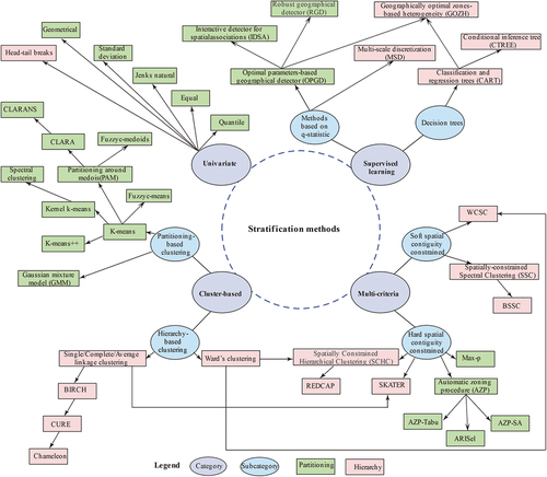
According to the study task (i.e. exploratory task or predictive task), the number of variables (univariate or multivariate) and the criterion of the algorithm (single criterion or multicriteria), we classify the stratification methods into four categories (Table 1), namely: univariate stratification, cluster-based stratification, multicriteria stratification, and supervised stratification.

Table 1. The categories of stratification methods.

	Exploratory task		Predictive task
	Single criterion	Multicriteria	-
Univariate	Univariate stratification	Multicriteria stratification	Supervised stratification
Multivariate	Cluster-based stratification

Figure 2 is the taxonomy of typical stratification methods under each category. In this section, we will provide detailed descriptions of the algorithms below.

Figure 2. Taxonomy of stratification methods (WCSC, Ward’s clustering with spatial constraints; BSSC, binarized spatially constrained spectral clustering; AZP-SA, AZP based on simulated annealing; ARiSel, automatic regionalization with initial seed location; SKATER, spatial “K”luster analysis by tree edge removal; REDCAP, regionalization with dynamically constrained agglomerative clustering and partitioning). The line with arrows between the two algorithms means that one is a variation of the other.

4.1. Univariate stratification

Univariate stratification methods are unsupervised and directly divide continuous data into user-defined parameters. The following is a description of the most commonly used univariate stratification methods (Cao, Ge, and Wang 2013; Song et al. 2020; Meng et al. 2021).

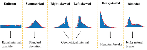
The equal interval (EI) divides the entire range of data values equally into specified intervals. The cut points depend only on the start and end points and on the number of groups, ignoring the distribution of the data.

The quantile (QU) divides data into specified intervals of equal size. The algorithm is distinctly useful for ordinal-level data. However, this may lead to objects of the same values being assigned to different strata, and values within-stratum may be hugely different.

The geometrical interval (GI) method creates geometrical intervals by minimizing the square sum of the elements per class, and the geometric coefficient in GI can change once (to its inverse) to optimize the class ranges, ensuring that each interval has approximately the same number of values. It is particularly suitable for data with skewed distribution, and the minimum value must be greater than zero.

The standard deviation (SD) is one of the stratification methods that considers data distribution. The breaks are formed by repeatedly adding or subtracting the standard deviation from the mean of the data. It only works well with symmetrically distributed data.

JNB is designed to determine the best arrangement of values into different intervals by minimizing the in-class variance and maximizing the inter-class variance (Fisher 1958; Jenks 1977). It is a good “general” method and has been the default classification method for ArcGIS, a popular platform for geographical information processing.

Head/tail breaks (HTB) (Jiang 2013) recursively separates data into head groups (greater than the mean) and tail groups (less than the mean), and then divides the head data into secondary heads and tails until the head part is no longer less than a threshold, such as 40%. The number of groups is determined by the threshold. HTB is a stratification scheme for data with a heavy-tailed distribution.

The break point of EI and GI is determined only by the start and end points (maximum and minimum values), and the SD by the mean and variance; therefore, in practice, it is necessary to carefully avoid creating invalid intervals when using EI, GI, or SD. Except for special demands (e.g. the quantile), how to choose from these methods is based on data distribution. Figure 3 summarizes the guidelines for choosing the method according to data distribution.

Figure 3. Univariate methods for stratification of corresponding data distributions.

4.2. Cluster-based stratification

Cluster-based stratification is aimed at grouping objects into strata based on their similarities. A large number of reviews about cluster analysis have been published, including general studies (Jain 2010; Xu and Wunsch 2005; Jain, Murty, and Flynn 1999) and studies on specific subjects, such as robustness of clustering (Angel Garcia-Escudero et al. 2010), spatiotemporal data clustering (Zhicheng and Pun-Cheng 2019), clustering for high-dimensional and large datasets (Pandove, Goel, and Rani 2018), clustering based on neural networks (Du 2010), and so on. Clustering algorithms can generally be classified as hierarchy-based or partitioning-based, according to the resultant partitions (Leung 2010; Jain, Murty, and Flynn 1999). Hierarchy-based methods generate a nested series of groups, while partitioning-based methods produce only one group.

4.2.1. Hierarchy-based clustering

Hierarchical clustering algorithms recursively find nested clusters in an agglomerative or divisive manner. Well-known agglomerative (bottom-up) algorithms include single linkage clustering (SLC), complete linkage clustering, and Ward’s linkage clustering (Ward 1963). For agglomerative hierarchical clustering, Lance and Williams (1967) proved a unified formula for dissimilarity updates:

where $d\left(x_i,x_j\right)$ is the distance of points $x_i$ and $x_j$ and ${\alpha }_i$, ${\alpha }_j$, $\beta ,$ and $\gamma$ define the agglomerative criteria, of which the settings in the above methods are shown in Table 2.

Table 2. Parameters of hierarchical clustering (Lance and Williams 1967).

Method	${\alpha }_i$	${\alpha }_j$	$\beta$	$\gamma$
Single linkage	1/2	1/2	0	−1/2
Complete linkage	1/2	1/2	0	1/2
Average linkage	$n_i/\left(n_i+n_j\right)$	$n_j/\left(n_i+n_j\right)$	0	0
Ward’s	$\frac{n_i+n_k}{n_i+n_j+n_k}$	$\frac{n_j+n_k}{n_i+n_j+n_k}$		0

Note: $n_i$ is the number of objects in stratum $i$

In contrast to agglomerative algorithms, divisive (top-down) algorithms are for splitting data rather than aggregating data and are always much more complex (Macnaughton-Smith et al. 1964); thus, they are rarely used for stratification. To manage time complexity (i.e. $O\left(n^{2}logn\right)$, where $n$ is the object size) and space complexity (i.e.) of agglomerative hierarchical clustering methods, scholars have proposed a few improved methods, such as the BIRCH (Zhang, Ramakrishnan, and Livny 1996), CURE (Guha, Rastogi, and Shim 1998), and Chameleon (Karypis, Han, and Kumar 1999).

The BIRCH is to compress data objects into many small subgroups and then cluster them. Since the number of subclusters after compressing is much smaller than the initial number of data objects, it allows cluster execution with a small memory, giving rise to algorithms that scan the database only once.

For CURE, random sampling and partitioning are used to reliably find clusters of arbitrary shapes and sizes. The minimum distance amid the representative points chosen is the cluster distance. This means that the technique incorporates both single-linkage and average-linkage methodologies.

The Chameleon algorithm groups objects into a number of small subclusters by a graphical partitioning algorithm under the given the minimum number of objects in a subcluster, and then finds the real clusters by repeating combinations of these subclusters with a hierarchical clustering algorithm. In Chameleon, cluster similarity is assessed by how well-connected objects are within a cluster and the closeness of clusters.

4.2.2. Partitioning-based clustering

Partitioning clustering is a grouping process that minimizes (or maximizes) an objective function (e.g. the sum of the squared errors of all clusters) and distinct from the hierarchical approach, it only gives a single partition of the dataset. K-means is the most famous partitioning clustering algorithm (Ball and Hall 1965; MacQueen 1967) and is also one of the most popular algorithms for geospatial clustering (Polczynski and Polczynski 2014; Huang et al. 2020). In K-means, a partition is identified when the sum of the squared error between the centroid and other points in the cluster is minimized and the centroid serves as the prototype.

Currently, most partitioning methods can be seen as an extension of the basic K-means, for example, the PAM (Kaufman and Rousseeuw 1990), the K-means++ (Arthur and Vassilvitskii 2007), etc. The K-means converge to local minima, and different initializations can lead to different final clustering. To overcome this weakness, K-means++ gives a different weight each time a new initial point is selected, and the weights depend on the distance from the previous initial point.

The PAM algorithm is more robust than K-means, in which each cluster is represented by the medoid, defined as the point with the least mean dissimilarity to all the points in the cluster. However, it cannot handle large datasets due to its high computational complexity. To compensate for this, CLARA (Clustering LARge Applications) was then proposed (Kaufman and Rousseeuw 1990). In CLARA, the medoids of a cluster are obtained with a sample from a set of objects, and then the remaining points are assigned to clusters where the nearest centroid is located; the cluster as the result is the one that performs best under different sample sets. CLARANS (Clustering Large Applications based on RANdomized Search) (Ng and Han 2002) is an improvement of both PAM and CLARA. In CLARANS, the process of grouping can be presented as searching a graph where every node is a potential solution, that is, a set of medoids. It is more effective than PAM because it checks only a sample of nodes. Unlike CLARA, CLARANS draws a sample of neighbors at each step of the search, which has the benefit of not confining a search to a local area.

By introducing a kernel distance function, the kernel K-means (Dhillon, Guan, and Kulis 2004; Schölkopf, Smola, and Müller 1998) addresses the limitation that K-means cannot capture the nonconvex structure of data. Spectral clustering is also an improvement for this limitation and is another nonlinear approach that acts on the eigenvectors of a matrix derived from the data. When inquiring into the relationship between the above two method, Dhillon, Guan, and Kulis (2004) found that the two classical spectral clustering methods – normalized cuts (Shi and Malik 2000) and NJW spectral clustering (Ng, Jordan, and Weiss 2001) – are special cases of weighted kernel K-means.

The Gaussian mixture model (Rasmussen 1999) is a well-known probability model-based algorithm. It assumes that all data points are generated from a mixture of a finite number of Gaussian distributions with unknown parameters. The mixture model can be regarded as a generalized K-means algorithm that contains information about the data covariance structure and potential Gaussian centers, which are usually estimated by the expectation maximization algorithm (Dempster, Laird, and Rubin 1977).

In the K-means and its variations mentioned in the previous paragraphs, each object belongs to one and only one group. Such crisp assignment of data to clusters can be inadequate in the presence of data points that are almost equally distant from two or more clusters. Fuzzy clustering allows objects to belong to more than one cluster simultaneously, with different degrees of membership in different clusters (for more details, see (D’Urso 2016)), and it is widely used in spatial analysis (D’Urso et al. 2019b; Coppi, D’Urso, and Giordani 2010). The famous fuzzy clustering is fuzzy c-means (FCM) (Bezdek 1981); Fuzzy c-medoids is very similar to the K-means except that the degree of fuzziness $df$ $(df>1)$ is needed. Fuzzy c-medoids is a variation of the PAM approach in a fuzzy framework with respect to the FCM, and it allows for more appeals and makes it easier to interpret the results of the final partition (D’Urso et al. 2019a).

4.3. Multicriteria stratification

Univariate methods and cluster-based methods mostly meet only one criterion of stratification, such as homogeneity (e.g. K-means) and balance size across strata (e.g. QU); thus, sometimes, they do not support stratification for spatial data, which were described by location and attributes (Cromley 1996; Jenks and Caspall 1971; Wise, Haining, and Ma 1997). A multicriteria stratification is desired in special application scenarios, such as climate zones (Fovell and Fovell 1993) and socioeconomic districts (AssunÇão et al. 2006). In addition to homogeneity, another most commonly used criterion is spatial contiguity (or spatial compactness). This section focuses mainly on regionalization methods, which are based on both homogeneity and spatial connectivity (Lankford 2010; Openshaw 1977; Gordon 1996b; Duque, Ramos, and Surinach 2007). According to whether explicit spatial connectivity constraint is satisfied, these methods can be categorized into two types: hard spatial contiguity-constrained stratification and soft spatial contiguity-constrained stratification.

4.3.1. Hard spatial contiguity-constrained stratification

Hard spatial contiguity entails that the objects of a stratum must be strictly geographically connected. In stratification, the spatial relationships of two datasets are represented by the spatial adjacency matrix, usually denoted by $\mathbf{W}=\left(w_{ij}\right),$ in which the $w_{ij}=1$ if the th and $j$ th unit are contiguous and ${\mathit{w}}_{\mathit{i}\mathit{j}}=0$ otherwise. Hard spatial contiguity-constrained stratification always maximizes the homogeneity of attributes under set constraints. Like clustering-based stratification, algorithms for hard spatial contiguity-constrained stratification can be divided into hierarchy-based and partitioning-based methods.

Hierarchy-based constrained stratification methods commonly used are spatially constrained hierarchical clustering (SCHC) (Guo 2009), spatial “K”luster analysis by tree edge removal (SKATER) (AssunÇão et al. 2006), and regionalization with dynamically constrained agglomerative clustering and partitioning (REDCAP) (Guo 2008). The SCHC is a special form of constrained clustering whose constraint is spatial contiguity, and the merged objects must be spatially contiguous. SKATER is based on a minimum spanning tree (MST) and is similar to a single-linkage cluster (Gower and Ross 1969). In SKATER stratification, a full graph is first created, with observations as nodes and contiguity relations as edges, and reduced to an MST. Finally, the MST is divided into regions; similar to SLC, SKATER has a “chaining effect.” REDCAP uses different ways to build the spanning tree based on three linkages (single linkage, average linkage, and complete linkage) and two spatial constraining strategies (first-order constraining and full-order constraining). First-order single linkage and SKATER are identical.

For partitioning-based methods, the common stratification methods are automatic zoning procedure (AZP) (Openshaw and Rao 1995; Openshaw 1977) and Max-p regionalization (Duque, Anselin, and Rey 2012). In AZP stratification, strata are divided when the sum of the squared errors of the continuous spatial variable data is minimized. It originally (Openshaw 1977) uses a slow hill-climbing heuristic to find the stratification solution, which has the problem of being trapped in a local solution. To promote this, Openshaw and Rao (1995) proposed two alternative approaches: the AZP-SA and the AZP-Tabu. The former employs the simulated annealing algorithm (Aarts and Korst 1989) as the optimal method, while the latter uses the Tabu Search algorithm (Glover 1986). Automatic regionalization with initial seed location (ARiSel) is a variant of AZP, choosing the best initial points among many starting points based on minimizing the sum of squared errors (Duque and Church 2004). The main disadvantage of AZP is its high computational cost and inability to process large datasets (Guo 2008). While, Max-p regionalization consists of three key phases: growth, assignment of enclaves, and spatial search. First, in the growth phase, based on equality under contiguity constraints, large neighbors are merged into start objects until the minimum bound is met. Second, areas that do not belong to divided regions are stored in enclaves. Lastly, these enclaves are assigned to existing regions based on homogeneity so that the overall within-group sum of squares is minimized. The Max-p stratification can automatically determine the number of partitions, but in it, equality has a greater impact than homogeneity.

4.3.2. Soft spatial contiguity-constrained stratification

The soft spatial contiguity implies that within-strata objects may not necessarily meet spatial connectivity, despite the consideration of geographical location or connectivity. There are two main solutions. The first takes the geographical coordinates (or centers of polygons) as additional attributes for clustering with different weights from other attributes (Webster and Burrough 1972; Oliver and Webster 1989). According to the weights given to the geographical coordinates and attributes, the results will have more or less spatially contiguous regions. However, it is challenging to set weights in applications. Ward’s clustering with spatial constraints proposed by Chavent et al. (2018) determines the weight of geographical similarity by increasing spatial contiguity without greatly decreasing the homogeneity of the feature space.

The other solution is to act on spatial connectivity by must-link or cannot-link constraints, resulting in a trade-off between spatial contiguity and homogeneity. Representative approaches include spectral constraint modeling (SCM) (Shi, Fan, and Philip 2010), spatially constrained spectral clustering (SSC), and binarized spatially constrained spectral clustering (BSSC) (Yuan et al. 2015). Yuan et al. (2015) has evaluated the effectiveness of SCM, SSC, and BSSC on a large-scale terrestrial ecology dataset and found that the SSC has the highest spatial connectivity (measured by the percentage of must-link constraints preserved within the regions) and moderate within-group sum-of-square error.

4.4. Supervised stratification

Supervised learning stratification methods are characterized by considering the study variable or existing labels in the process of stratification, which makes more helpful predictions than unsupervised learning methods. When objects have been labeled, many supervised learning algorithms can be used for stratification (Ramírez‐Gallego et al. 2015; Yang, Webb, and Wu 2009). In this section, we introduce the regression decision trees and methods based on the q-statistic in the geographical detector.

4.4.1. Decision trees

Decision trees are nonparametric-supervised learning methods used for classification and regression. Classification and regression trees (CART) (Breiman et al. 1984) does not require data scaling or normalization, and variables can be both continuous and discrete. In CART, exploratory variables are recursively partitioned into strata that are as homogeneous as possible with respect to the study variable. CART grows a large tree and then prunes the tree to a size based on a cross-validation error. The conditional inference tree (CTREE) (Hothorn, Hornik, and Zeileis 2006), a regression method, recursively splits the space of exploratory variables based on the $p$-value of the difference of study variables between partitions from permutation distributions. The tree size (i.e. the number of strata) of CTREE was controlled by the threshold of the given significance level. Many other regression tree models are also applicable for stratification; a relatively well-rounded overview can be found in Loh (2014).

4.4.2. Methods based on the q-statistic

The q-statistic of the geographical detector can be used to measure the SSH (Wang et al. 2010; Wang, Zhang, and Fu 2016). It considers the study space to be composed of $n$ spatial objects, stratified into strata; stratum $k$ is composed of spatial objects, and $y_i$ and $y_{hi}$ denote the study variable value of unit in the population and in stratum $h$, respectively:

(4) $q=1-\frac{{\sum }_{h=1}^L{\sum }_{i=1}^{n_h}{\left(y_{hi}-{\bar{y}}_h\right)}^2}{{\sum }_{i=1}^n{\left(y_i-\bar{y}\right)}^2}$(4)

The objective function is expressed as follows:

(5) $\begin{array}{c}\underset{X_h}{\mathrm{a}\mathrm{r}\mathrm{g}\mathrm{m}\mathrm{a}\mathrm{x}}\mathrm{q}=\underset{X_h}{\mathrm{a}\mathrm{r}\mathrm{g}\mathrm{m}\mathrm{i}\mathrm{n}}{\sum }_{h=1}^L{\sum }_{i=1}^{n_h}{\left(y_{hi}-{\bar{y}}_h\right)}^2\end{array}$(5)

Methods of q-statistic-based stratification are the optimal parameter-based geographical detector (OPGD) (Song et al. 2020), the multi-scale discretization (MSD) (Meng et al. 2021), the interactive detector for spatial associations (IDSA) (Song and Wu 2021), the geographically optimal zone-based heterogeneity (GOZH) algorithm (Luo et al. 2022), and the robust geographical detector (RGD) (Zhang, Song, and Wu 2022). The OPGD needs to be given the number of strata intervals and grouping methods; it then selects the highest q-statistic value result among all combinations of the interval and methods as the final stratification scheme. The MSD uses upscale and downscale strategies to obtain the optimal cut points that maximize the q-statistic value, with the advantage that the result is dependent on the characteristics of the explanatory variables and the study variable. The IDSA employs spatial fuzzy overlay, a process for overlapping geographical variables, to derive spatial zones in terms of fuzzy relations across spaces. Compared with OPGD, stratification in IDSA accounts for the correlations between stratification variables. GOZH employs CART to generate interactive strata in which the number of strata is less than those by spatial overlays in the geographical detector. The RGD motivated by the q-statistic is sensitive to the stratification of explanatory variables, in which the optimization algorithm for variance-based change point detection obtains a robust q-statistic.

5. Selection of stratification methods

5.1. Stratification algorithm comparison

As shown in Figure 2, some algorithms inherit and improve upon root characteristics of root algorithms. Improvements are mainly in robustness – the ability to resist the effects of outliers, arbitrary shape, spatial contiguity, stability, and scalability to large data. Stability means that the results of stratification are rarely influenced by the initial conditions, for example, the enhancement of the K-means++ to the K-means. The scalability of large data refers to the fact that the run time and memory requirements should not explode for large datasets (Andreopoulos et al. 2009).

In Table 3, we have summarized the general characteristics of the stratification methods from the input data, input parameters, robustness, arbitrary shape, and scalability to large data. A good stratification algorithm should have less input parameters, be less sensitive to outliers, support arbitrary shape and have scalability to large data.

Table 3. Stratification algorithm comparison.

Methods	References	Input Data	Input parameters	Robust to outliers	Arbitrary shape	Scalability to large data	Software packages
Univariate stratification
EI/QU/JNK/SD	Jenks (1977)	X	NS	No	-	-	Arcgis, QGIS, classInt (R), mapclassify (Python)
GI		X	NS	No	-	-	Arcgis
HTB	Jiang (2013)	X	Stop threshold	No	-	-	classInt (R), mapclassify (Python)
Cluster-based stratification
K-means	MacQueen (1967)	$X$	NS; Stop threshold	No	No	Yes	Geoda, stats (R), Scikit-learn (Python)
Partitioning around medoids	Kaufman and Rousseeuw (1990)	$X$	NS	Yes	Yes	No	cluster(R), Scikit-learn (Python)
CLARA	Kaufman and Rousseeuw (1990)	$X$	NS, number of samples	Yes	Yes	Yes	cluster(R), PyClustering (Python)
CLARANS	Ng and Han (2002)		NS, numlocal, maxneight	Yes	Yes	Yes	cluster(R), PyClustering (Python)
Fuzzy c-means		$X$	NS,	No	Yes	Yes	R, Python
K-means++	Arthur and Vassilvitskii (2007)	$X$	NS	No	No	Yes	Geoda, stats(R), Scikit-learn (Python)
Kernel-k-means	Dhillon, Guan, and Kulis (2004)	$X$	NS, degree of fuzziness	Yes	Yes	No	kernlab (R)
Spectral clustering	Shi and Malik (2000) Ng, Jordan, and Weiss (2001)	DM	NS	Yes	Yes	No	Geoda, kernlab (R), Scikit-learn (Python)
Agglomerative single-linkage clustering	Florek et al. (1951)	DM	NS	Yes	Yes	No	Geoda, stats (R), Scikit-learn (Python)
Agglomerative complete-linkage clustering	McQuitty (1960)	DM	NS	Yes	Yes	No	stats (R), Python, Geoda
Agglomerative average-linkage clustering	McQuitty (1967)	DM	NS	Yes	Yes	No	stats (R), Python, Geoda
Ward’s clustering	Ward (1963)	DM	NS	No	No	No	stats (R), Python, Geoda
Gaussian mixed model	Rasmussen (1999)	$X$	NS; stop threshold	No	No	Yes	mclust (R), Python
BIRCH	Zhang, Ramakrishnan, and Livny (1996)	$X$	NS; maxCF	Yes	No	Yes	Scikit-learn (Python),
CURE	Guha, Rastogi, and Shim (1998)	$X$	NS; numrep	Yes	Yes	Yes	PyClustering (Python)
Chameleon	Karypis, Han, and Kumar (1999)	$X$	numlocal; minsize; $a$	Yes	Yes	Yes	seriation (R)
Multicriteria stratification
Automatic zoning procedure (AZP) /AZP-SA/AZP-Tabu	Openshaw (1977) Openshaw and Rao (1995)	$X$	NS, SW	No	No	No	Geoda, spot (python)
ARISeL	Duque and Church (2004)	$X$	NS, SW	No	No	No	Geoda, spot (python)
SKATER	AssunÇão et al. (2006),	DM	NS, SW	No	Yes	No	Arcgis, Geoda, spdep (R), spot (python)
REDCAP	Guo (2008)	DM	NS, SW	Yes	Yes	No	Geoda, spot(python)
Ward’s clustering with spatial constraints	Chavent et al. (2018)	DM	NS, SW	No	Yes	No	ClustGeo (R)
Spatially-constrained spectral clustering	Yuan et al. (2015)	DM	NS, SW	Yes	Yes	No	Code
Max-p Regionalization	Duque, Anselin, and Rey (2012)	$X$	SW; threshold of spatially extensive regional attribute	No	No	No	Geoda, spot (python)
Supervised stratification
Classification and regression trees	Breiman et al. (1984)	$X$, $y$	minsplit, complexity parameter	No	-	Yes	rpart (R), Scikit-learn (Python),
Conditional inference tree	Hothorn, Hornik, and Zeileis (2006)	$X$, $y$	minsplit, significance level for split	No	-	Yes	rpartkit(R)
Optimal parameter-based geographical detector	Song et al. (2020)	$X$, $y$	NS interval, univariable stratification methods	No	-	Yes	GD (R)
Multi-scale discretization	Meng et al. (2021)	$X$, $y$	NS, upscaling number, buffer scale number	No	-	No	Code
Interactive detector for spatial associations	Song and Wu (2021)	$X$, $y$	Spatial location, NS interval, univariable stratification methods	No	-	Yes	ISDA (R)
Geographically optimal zone-based heterogeneity	Luo et al. (2022)	$X$, $y$	minsplit, complexity parameter	No	-	Yes	rpart (R), GD (R)
Robust geographical detector	Zhang, Song, and Wu (2022)	$X$, $y$	NS	Yes	-	Yes	Code

$X=\left\{x_i\right\},i=1,\dots ,n$ be the set of $d$-dimensional points, n is objects size, and $d$ is variables size; $y=\left\{y_i\right\}$ is the study variable; NS, number of strata; SW, spatial weights; DM, distance (dissimilarity) matrix; numlocal, number of local minima; maxneighbor, maximum number of neighbors; maxCF, maximum number of CF subclusters in each node; numrep, number of representative points for each stratum; minsize, threshold of number of vertices; $a$, important indicator for the relative closeness and relative inter-connectivity; minsplit, the minimum number of observations that must exist in a node; classInt (R), means the classInt is a R package; mapclassify (Python), means the mapclassify is a Python package.

This information in Figure 2 Table 3 will help users to better select the appropriate method for an application. Although the improved method has better performance in some respects than the original one, it may also lose simplicity, i.e. it requires more input parameters; so, in practical applications, it is necessary not only to meet the problem requirements but also to consider the difficulty of parameter selection. For example, in the Chameleon algorithm, although the method can identify clusters better, it requires us to input four parameters, and the parameter selection process has a significant impact on the results.

5.2. The number of strata

One of the most difficult issues for stratification is defining an appropriate number of strata is of great importance for unsupervised stratification. Although some algorithms, such as head/tail breaks and max-p regionalization, do not need to set the number of strata, they still need to input other parameters to decide it. A reasonable solution we suggest is to first set the interval of the number of strata (e.g. to match the human memory limit, the number should not exceed nine (Miller 1994)) and then select “optimal” number from the interval with the help of statistical indices or visualizations.

Many indices can be used to determine the number of strata (Milligan and Cooper 1985; Gordon 1996a; Liu et al. 2010), and they can be grouped into two classes. One class includes indices based on the compactness of within stratum objects (or separability of strata), for example, the Calinski–Harabasz index (CH) (Caliński and Harabasz 1974), the silhouette correlation (SC) index (Rousseeuw 1987), and gap statistics (Tibshirani, Walther, and Hastie 2001); the other includes indices based on cluster stability (Wang 2010; Ben-David, von Luxburg, and Pál 2006), which are always achieved by cross-validation or bootstrapping (Fang and Wang 2012). In Table 4, we listed four famous statistical metrics for choosing the best number of strata. The CH index (Caliński and Harabasz 1974) is a computationally efficient and the most commonly used non-supervisory evaluation metric (Milligan and Cooper 1985). The gap statistics and clustering stability-based methods are more general than CH and SC.

Table 4. Statistical metrics for determining the number of strata.

Measure	Definition	Optimal value
Calinski-Harabasz index	$\mathrm{C}\mathrm{H}\left(k\right)=\frac{{\sum }_{p=1}^k{n}_p||c_p-\mathrm{c}|{|}^2/\left(k-1\right)}{{\sum }_{p=1}^k{\sum }_{x_i\in S_p}||x_i-c_p|{|}^2/\left(n-k\right)}$	Max
Silhouette index	$\frac{1}{n}\sum (i=1)n\frac{b(x_i)-a(x_i)\}}{max(b(x_i),a(x_i))}$$a(i)=\frac{1}{n_p-1}\sum _{xi,xj\in s_p}d(xi,xj)$, $b(i)=\underset{q\ne p,}{min}(\frac{1}{n_q}\sum _{x_i\in S_p,j\in S_q}d(x_i,x_j))$	Max
Gap statistics	$Ga{p}_n(k)=E_n^{\ast }\left(\mathrm{l}\mathrm{o}\mathrm{g}(W_k\right))-\mathrm{l}\mathrm{o}\mathrm{g}(W_k)$,$Ga{p}_n(k)\ge Ga{p}_n(k+1)-\sqrt{1+1/B}s{d}_k$$W_k=\sum _{(p=1)}^k\left(\frac{1}{2n_p}\sum _{i,j\in S_p}d(x_i,x_j)\right),E_n^{\ast }(log(W_k))$ = $1/B\sum _{b}log({W_{kb}}^{\ast }))$, $\mathrm{s}{\mathrm{d}}_k=[\left(1/B\right)\sum _b{\left\{\mathrm{l}\mathrm{o}\mathrm{g}(W_{kb}^{\ast })-E_n^{\ast }\left(\mathrm{l}\mathrm{o}\mathrm{g}(W_k\right))\right\}}^2{]}^{1/2}$	Elbow
Clustering stability	$\frac{1}{B{n}^2}\sum _{b=1}^B\sum _{i=1}^n\sum _{j=1}^n|I\{S_{X_b^{\ast n},k}(x_i)=S_{X_b^{\ast n},k}(x_j)\}-I\{S_{{\hat{X}}_b^{\ast n},k}(x_i)=S_{{\hat{X}}_b^{\ast n},k}(x_j)\}|$	Min

Note: $c$: center of data, $S_p$, $p$-th stratum; $n_p$: number of objects in $s_p$; $c_p$ center of data of $S_p{d}_{ij}$: distance between object $i$ and $j$; B bootstrap number; $I\left\{.\right\}$: indicator function; $b=1,2,..,B$ is the bootstrap index. ($X_b^{\ast n},{\hat{X}}_b^{\ast n}$): bootstrap sample-pairs.

Visualization of data is also an important means for determining the number of strata, of which the most common ones are histograms for one-dimensional data and scatterplots for two-dimensional data. Meanwhile, there are many techniques for mapping high-dimensional data to lower-dimensional data, including linear projection methods, such as principal component analysis (Wold, Esbensen, and Geladi 1987) and multidimensional scaling (MDS) (Sammon 1969), and nonlinear projection methods, such as self-organizing mapping (Kohonen 1990). In addition to the projection methods, visual assessment of tendency (VAT) can be also used to identify the number of strata by reordering the dissimilarity matrix for the data so that similar samples are placed close to each other (Bezdek and Hathaway 2002). A detailed overview of the VAT family of algorithms can be found in a study by Dheeraj and Bezdek (2020).

5.3. Software packages

Many stratification software packages are available in R (R Core Team 2021), Python, ArcGIS, QGIS, and Geoda (Anselin, Syabri, and Kho 2010) for spatial data. For univariate stratification, the base packages are classInt (Bivand et al. 2013) in R and mapclassify in Python. The mapclassify is a subpackage of the Python Spatial Analysis Library (PySAL) (Rey and Anselin 2010). The cluster-based stratification packages are stats and cluster (Maechler et al. 2012) in R, and Scikit-learn (Pedregosa et al. 2011) and pyclustering (Novikov 2019) in Python. Other R cluster analysis packages not mentioned in this study can be found at Comprehensive R Archive Network task views (https://cran.r-project.org/web/views/Cluster.html). Generally, most spatially constrained stratification methods can be implemented with PySAL, Geoda. The software packages are summarized in Table 3.

6. Discussion

6.1. Assessment of strata

Assessment of the results is critical, especially when the strata is used for later sampling and inference, etc. For supervised stratification methods, the assessment of output is simple, and we can use the sum squared errors (SSE) of study variable or q-statistic in Equation 4(4) $q=1-\frac{{\sum }_{h=1}^L{\sum }_{i=1}^{n_h}{\left(y_{hi}-{\bar{y}}_h\right)}^2}{{\sum }_{i=1}^n{\left(y_i-\bar{y}\right)}^2}$(4) . The advantage of q-statistic is its value within [0,1], which also can be index of association between continues study variables and categorical explanatory variable. To avoid overfitting, the SSE or q-statistic can be calculated by cross-validation. For unsupervised stratification methods, the assessment is not trivial as supervised algorithm because the context should be taken into account, that is the assessment of unsupervised stratification should be based on the study context as well as statistical indicators. The classical statistical indicators to quantify inter-strata similarity, or intra-strata dissimilarity are SSE of explanatory variables (i.e. within-strata variability in Equation $6$) and SH index which was described in Table 5. The other metrics can be found in literatures such as (Milligan and Cooper 1985), Gordon (1996a), and (Liu et al. 2010).

6.2. Limitations of this study

All the methods listed in this paper are of general purpose, not focusing on the special domains in which superior stratification should be based on a priori knowledge to ensure that the results have good interpretation power. However, in practical applications, prior knowledge does not always exist, so it is necessary to use algorithms based on data distribution and given constraints. In this paper, we introduce the characteristics of different methods but do not provide a scenario to be used strictly by individuals because, in practice, it is difficult to have a reliable evaluation index for unsupervised methods. More conventional methods and the degree of difficulty of method implementation are preferred. For example, in the application of the geographical detector model, a popular tool for SSH analysis, the top three most popular stratification algorithms are JNB, K-means, and quantile (Meng et al. 2021).

6.3. Future recommendations

Although SSH has been widely used in many fields, few studies have been conducted on new theoretical approaches to SSH. In the future, research should be furthered in the following four aspects. The first is how to synthesize the stratification of multiple variables in practical applications. The available methods are clustering and spatial overlays of each variable stratum (Wang et al. 2010). The former ignores the importance of variables, and the latter may cause a “curse of dimensionality” (Bellman 1966) – the number of strata would expand exponentially with increasing variables, and many strata would end up devoid of samples and thus be incapable of providing any probability estimates. The second is how to evaluate the uncertainty of stratification in subsequent sampling or modeling. The third is developing new measures of SSH. The q-statistic and spatial association detector (a variation of q-statistic) (Cang and Luo 2018) are applicable only for univariate analysis and crisp strata. Future research is urgently needed to develop SSH measures for spatial multivariate data and/or fuzzy strata. The last is building new stratification algorithm or prediction models based on both spatial autocorrelation and SSH, which are two main ways to describe spatial variation.

7. Conclusions

SSH, a fundamental assumption for understanding geographical objects, simplifies a complex object, explains nonlinear relationships between variables, and eliminates confounding factors in modeling by stratification. In stratification, different algorithms reflect distinct human understandings of spatial distributions and associations. The choice of stratification depends on the task of stratification (e.g. exploratory task should use the unsupervised stratification and the predictive task should use the supervised stratification) and on the study context that may involve in the specific constraints. No method is optimal in a general sense, and knowledge of the different characteristics of an algorithm is important for making the required decisions. We have summarized typical existing stratification methods and constructed a taxonomy for selecting a more reasonable method. If the number of strata is otherwise unknown, statistical metrics and the visualization approach are proved to be helpful in selecting an appropriate number of strata. The scale dependence of SSH remains a challenge in earth science and requires further study. Future research is recommended to reveal the nature of geographical attributes through the integration of SSH, advanced measures for multivariate analysis and/or fuzzy strata, and new prediction models based on spatial autocorrelation and SSH.

Data availability statement

The simulation data that support the findings of this study are available at https://github.com/geogxy/modelling_ssh

Disclosure statement

No potential conflict of interest was reported by the author(s).

Additional information

Funding

This work was supported by the National Natural Science Foundation of China [42071375].

References

- Aarts, E., and J. Korst. 1989. Simulated Annealing and Boltzmann Machines: A Stochastic Approach to Combinatorial Optimization and Neural Computing. New York: John Wiley & Sons.
- Andreopoulos, B., A. Aijun, X. Wang, and M. Schroeder. 2009. “A Roadmap of Clustering Algorithms: Finding A Match for A Biomedical Application.” Briefings in Bioinformatics 10 (3): 297–314. doi:10.1093/bib/bbn058.
- Anselin, L. 1995. “Local Indicators of Spatial Association - Lisa.” Geographical Analysis 27 (2): 93–115. doi:10.1111/j.1538-4632.1995.tb00338.x.
- Anselin, L., I. Syabri, and Y. Kho. 2010. “GeoDa: An Introduction to Spatial Data Analysis.” In Handbook of Applied Spatial Analysis, 73–89. Berlin, Heidelberg: Springer.
- Armstrong, M. P., N. Xiao, and D. A. Bennett. 2003. “Using Genetic Algorithms to Create Multicriteria Class Intervals for Choropleth Maps.” Annals of the Association of American Geographers 93 (3): 595–623. doi:10.1111/1467-8306.9303005.
- Arthur, D., and S. Vassilvitskii. 2007. “K-means++: The Advantages of Careful Seeding.” Proceedings of the eighteenth annual ACM-SIAM symposium on Discrete algorithms, 1027–1035. New Orleans, Louisiana: Society for Industrial and Applied Mathematics.
- AssunÇão, R. M., M. C. Neves, G. Câmara, and C. Da Costa Freitas. 2006. “Efficient Regionalization Techniques for Socio‐economic Geographical Units Using Minimum Spanning Trees.” International Journal of Geographical Information Science 20 (7): 797–811. doi:10.1080/13658810600665111.
- Bailey, R. G. 1995. Description of the Ecoregions of the United States. Forest Service: US Department of Agriculture.
- Ball, G. H., and D. J. Hall. 1965. “ISODATA: A novel method of data analysis and pattern classification.” Technical report NTIS AD 699616. Stanford Research Institute, Stanford, CA.
- Bellman, R. 1966. “Dynamic Programming.” Science 153 (3731): 34–37. doi:10.1126/science.153.3731.34.
- Ben-David, S., U. von Luxburg, and D. Pál. 2006. “A Sober Look at Clustering Stability.” In Learning Theory. Berlin, Heidelberg: Springer. doi:10.1007/11776420_4.
- Bezdek, J. C. 1981. Pattern Recognition with Fuzzy Objective Function Algorithms. New York, NY: Springer.
- Bezdek, J. C., and R. J. Hathaway. 2002. “VAT: A Tool for Visual Assessment of (Cluster) Tendency.” Paper presented at the Proceedings of the 2002 International Joint Conference on Neural Networks. IJCNN’02 (Cat. No. 02CH37290), Honolulu, HI, USA.
- Bivand, R., H. Ono, R. Dunlap, and M. Stigler. 2013. “classInt: Choose Univariate Class Intervals.” Url R package version 0.1–21. http://CRAN.R-project.org/package=classInt
- Breiman, L., J. H. Friedman, R. A. Olshen, and C. J. Stone. 1984. Classification And Regression Trees, Wadsworth Inc. New York: Routledge.
- Brunsdon, C., S. Fotheringham, and M. Charlton. 1998. “Geographically Weighted Regression.” Journal of the Royal Statistical Society: Series D (The Statistician) 47 (3): 431–443. doi:10.1111/1467-9884.00145.
- Caliński, T., and J. Harabasz. 1974. “A Dendrite Method for Cluster Analysis.” Communications in Statistics-Theory and Methods 3 (1): 1–27. doi:10.1080/03610927408827101.
- Cang, X. Z., and W. Luo. 2018. “Spatial Association Detector (SPADE).” International Journal of Geographical Information Science 32 (10): 2055–2075. doi:10.1080/13658816.2018.1476693.
- Cao, F., Y. Ge, and J. F. Wang. 2013. “Optimal Discretization for Geographical detectors-based Risk Assessment.” Giscience & Remote Sensing 50 (1): 78–92. doi:10.1080/15481603.2013.778562.
- Chavent, M., V. Kuentz-Simonet, A. Labenne, and J. Saracco. 2018. “ClustGeo: An R Package for Hierarchical Clustering with Spatial Constraints.” Computational Statistics 33 (4): 1799–1822. doi:10.1007/s00180-018-0791-1.
- Cochran, W. G. 1977. Sampling Techniques. 3rd ed. New York: John Wiley & Sons.
- Coppi, R., P. D’Urso, and P. Giordani. 2010. “A Fuzzy Clustering Model for Multivariate Spatial Time Series.” Journal of Classification 27 (1): 54–88. doi:10.1007/s00357-010-9043-y.
- Cromley, R. G. 1996. “A Comparison of Optimal Classification Strategies for Choroplethic Displays of Spatially Aggregated Data.” International Journal of Geographical Information Systems 10 (4): 405–424. doi:10.1080/02693799608902087.
- Dempster, A. P., N. M. Laird, and D. B. Rubin. 1977. “Maximum Likelihood from Incomplete Data via the EM Algorithm.” Journal of the Royal Statistical Society: Series B (Methodological) 39 (1): 1–22. doi:10.1111/j.2517-6161.1977.tb01600.x.
- Deza, M. M., and E. Deza. 2016. Encyclopedia of Distances. Berlin, Heidelberg: Springer.
- Dheeraj, K., and J. C. Bezdek. 2020. “Visual Approaches for Exploratory Data Analysis: A Survey of the Visual Assessment of Clustering Tendency (VAT) Family of Algorithms.” IEEE Systems, Man, and Cybernetics Magazine 6 (2): 10–48. doi:10.1109/msmc.2019.2961163.
- Dhillon, I. S., Y. Q. Guan, and B. Kulis. 2004. “Kernel k-means.” Proceedings of the 2004 ACM SIGKDD international conference on Knowledge discovery and data mining - KDD ‘04, 551–556. Seattle, WA, USA: Association for Computing Machinery.
- Du, K. L. 2010. “Clustering: A Neural Network Approach.” Neural Networks 23 (1): 89–107. doi:10.1016/j.neunet.2009.08.007.
- Duda, R. O., P. E. Hart, and D. G. Stork. 2000. Pattern Classification. 2nd ed. New York: John Wiley & Sons.
- Duque, J. C., L. Anselin, and S. J. Rey. 2012. “The Max-P-Regions Problem*.” Journal of Regional Science 52 (3): 397–419. doi:10.1111/j.1467-9787.2011.00743.x.
- Duque, J. C., and R. L. Church. 2004. “A New Heuristic Model for Designing Analytical Regions.” Paper presented at the North American Meeting of the International Regional Science Association, Seattle.
- Duque, J. C., R. Ramos, and J. Surinach. 2007. “Supervised Regionalization Methods: A Survey.” International Regional Science Review 30 (3): 195–220. doi:10.1177/0160017607301605.
- D’Urso, P. 2016. “Fuzzy Clustering.“ In Handbook of Cluster Analysis. New York: Chapman and Hall/CRC.
- D’Urso, P., L. De Giovanni, M. Disegna, and R. Massari. 2019a. “Fuzzy Clustering with spatial–temporal Information.” Spatial Statistics 30: 71–102. doi:10.1016/j.spasta.2019.03.002.
- D’Urso, P., G. Manca, N. Waters, and S. Girone. 2019b. “Visualizing Regional Clusters of Sardinia’s EU Supported Agriculture: A Spatial Fuzzy Partitioning around Medoids.” Land Use Policy 83: 571–580. doi:10.1016/j.landusepol.2019.01.030.
- Dutilleul, P., and P. Legendre. 1993. “Spatial Heterogeneity against Heteroscedasticity: An Ecological Paradigm versus a Statistical Concept.” Oikos 66 (1): 152–171.
- Fang, Y. X., and J. H. Wang. 2012. “Selection of the Number of Clusters via the Bootstrap Method.” Computational Statistics & Data Analysis 56 (3): 468–477. doi:10.1016/j.csda.2011.09.003.
- Fisher, W. D. 1958. “On Grouping for Maximum Homogeneity.” Journal of the American Statistical Association 53 (284): 789–798. doi:10.1080/01621459.1958.10501479.
- Florek, K., J. Łukaszewicz, J. Perkal, H. Steinhaus, and S. Zubrzycki. 1951. “Sur la liaison et la division des points d’un ensemble fini.” Paper presented at the Colloquium Mathematicum.
- Fotheringham, A. S., W. Yang, and W. Kang. 2017. “Multiscale Geographically Weighted Regression (MGWR).” Annals of the American Association of Geographers 107 (6): 1247–1265. doi:10.1080/24694452.2017.1352480.
- Fovell, R. G., and M. Y. C. Fovell. 1993. “Climate Zones of the Conterminous United-States Defined Using Cluster-Analysis.” Journal of Climate 6 (11): 2103–2135. doi:10.1175/1520-0442(1993)006<2103:CZOTCU>2.0.CO;2.
- Gaetan, C., and X. Guyon 2010. “Spatial Statistics and Modeling.” In Springer Series in Statistics. Vol. 90. New York, NY: Springer.
- Gao, B., H. Maogui, J. Wang, X. Chengdong, Z. Chen, H. Fan, and H. Ding. 2020. “Spatial Interpolation of Marine Environment Data Using P-MSN.” International Journal of Geographical Information Science 34 (3): 577–603. doi:10.1080/13658816.2019.1683183.
- Garcia-Escudero, A., A. G. Luis, C. Matran, and A. Mayo-Iscar. 2010. “A Review of Robust Clustering Methods.” Advances in Data Analysis and Classification 4 (2–3): 89–109. doi:10.1007/s11634-010-0064-5.
- Getis, A., and J. K. Ord. 1992. “The Analysis of Spatial Association by Use of Distance Statistics.” Geographical Analysis 24 (3): 189–206. doi:10.1111/j.1538-4632.1992.tb00261.x.
- Glover, F. 1986. “Future Paths for Integer Programming and Links to Artificial-Intelligence.” Computers & Operations Research 13 (5): 533–549. doi:10.1016/0305-0548(86)90048-1.
- Gordon, A. D. 1996a. “Null Models in Cluster Validation.” Paper presented at the From Data to Knowledge, Berlin, Heidelberg.
- Gordon, A. D. 1996b. “A Survey of Constrained Classification.” Computational Statistics & Data Analysis 21 (1): 17–29. doi:10.1016/0167-9473(95)00005-4.
- Gower, J. C., and G. J. S. Ross. 1969. “Minimum Spanning Trees and Single Linkage Cluster Analysis.” Journal of the Royal Statistical Society: Series C (Applied Statistics) 18 (1): 54–64.
- Guha, S., R. Rastogi, and K. Shim. 1998. “CURE: An Efficient Clustering Algorithm for Large Databases.” ACM SIGMOD Record 27 (2): 73–84. doi:10.1145/276305.276312.
- Guo, D. S. 2008. “Regionalization with Dynamically Constrained Agglomerative Clustering and Partitioning (REDCAP).” International Journal of Geographical Information Science 22 (7): 801–823. doi:10.1080/13658810701674970.
- Guo, D. S. 2009. “Greedy Optimization for contiguity-constrained Hierarchical Clustering.” Paper presented at the 2009 IEEE International Conference on Data Mining Workshops, Miami, FL, USA.
- Guo, D. S., and H. Wang. 2011. “Automatic Region Building for Spatial Analysis.” Transactions in GIS 15: 29–45. doi:10.1111/j.1467-9671.2011.01269.x.
- Hess, S. W., and S. A. Samuels. 1971. “Experiences with a Sales Districting Model: Criteria and Implementation.” Management Science 18 (4–part–ii): 41. doi:10.1287/mnsc.18.4.P41.
- Hothorn, T., K. Hornik, and A. Zeileis. 2006. “Unbiased Recursive Partitioning: A Conditional Inference Framework.” Journal of Computational and Graphical Statistics 15 (3): 651–674. doi:10.1198/106186006x133933.
- Huang, Z., Y. Lu, E. A. Mack, W. Chen, and R. Maciejewski. 2020. “Exploring the Sensitivity of Choropleths under Attribute Uncertainty.” IEEE transactions on Visualization and Computer Graphics 26 (8): 2576–2590. doi:10.1109/TVCG.2019.2892483.
- Huang, B., B. Wu, and M. Barry. 2010. “Geographically and Temporally Weighted Regression for Modeling spatio-temporal Variation in House Prices.” International Journal of Geographical Information Science 24 (3): 383–401. doi:10.1080/13658810802672469.
- Hu, M. G., H. Lin, J. F. Wang, C. D. Xu, A. Tatem, B. Meng, X. Zhang, et al. 2020. “The Risk of COVID-19 Transmission in Train Passengers: An Epidemiological and Modelling Study.” Clinical Infectious Diseases 71 (1): 72. doi:10.1093/cid/ciaa1057.
- Jain, A K. 2010. “Data Clustering: 50 Years beyond K-means.” Pattern Recognition Letters 31 (8): 651–666. doi:10.1016/j.patrec.2009.09.011.
- Jain, A. K., M. N. Murty, and P. J. Flynn. 1999. “Data Clustering: A Review.” Acm Computing Surveys 31 (3): 264–323. doi:10.1145/331499.331504.
- Jenks, G. F. 1977. “Optimal Data Classification for Choropleth Maps.” Department of Geographiy Occasional Paper. Lawrence: University of Kansas.
- Jenks, G. F., and F. C. Caspall. 1971. “Error on Choroplethic Maps: Definition, Measurement, Reduction.” Annals of the Association of American Geographers 61 (2): 217–244. doi:10.1111/j.1467-8306.1971.tb00779.x.
- Jiang, B. 2013. “Head/Tail Breaks: A New Classification Scheme for Data with A Heavy-Tailed Distribution.” The Professional Geographer 65 (3): 482–494. doi:10.1080/00330124.2012.700499.
- Kaiser, H. F. 1966. “An Objective Method for Establishing Legislative Districts.” Midwest Journal of Political Science 10 (2): 200–213.
- Karypis, G., E.-H. Han, and V. Kumar. 1999. “Chameleon: Hierarchical Clustering Using Dynamic Modeling.” Computer 32 (8): 68–75. doi:10.1109/2.781637.
- Kaufman, L., and P. J. Rousseeuw. 1990. “Partitioning Around Medoids (Program PAM).” In Finding Groups in Data: An Introduction to Cluster Analysis, 68-125. Hoboken, New Jersey: John Wiley & Sons.
- Kohonen, T. 1990. “The self-organizing Map.” Proceedings of the IEEE 78 (9): 1464–1480.
- Köppen, W. 1931. Grundriß der Klimakunde. Berlin: De Gruyter.
- Kulldorff, M. 1997. “A Spatial Scan Statistic.” Communications in Statistics-Theory and Methods 26 (6): 1481–1496. doi:10.1080/03610929708831995.
- Lance, G. N., and W. T. Williams. 1967. “A General Theory of Classificatory Sorting Strategies: 1. Hierarchical Systems.” the Computer Journal 9 (4): 373–380. doi:10.1093/comjnl/9.4.373.
- Lankford, P. M. 2010. “Regionalization: Theory and Alternative Algorithms.” Geographical Analysis 1 (2): 196–212. doi:10.1111/j.1538-4632.1969.tb00615.x.
- Leung, Y. 2010. Knowledge Discovery in Spatial Data. Berlin, Heidelberg: Springer.
- Liu, Y., Y. Chen, Z. F. Wu, B. Wang, and S. Wang. 2021. “Geographical detector-based Stratified Regression Kriging Strategy for Mapping Soil Organic Carbon with High Spatial Heterogeneity.” Catena 196: 104953. doi:10.1016/j.catena.2020.104953.
- Liu, Y., Z. Li, H. Xiong, X. Gao, and J. Wu. 2010. “Understanding of Internal Clustering Validation Measures.” Paper presented at the 2010 IEEE International Conference on Data Mining, Sydney, NSW, Australia.
- Loh, W. Y. 2014. “Fifty Years of Classification and Regression Trees.” International Statistical Review 82 (3): 329–348.
- Luo, P., Y. Z. Song, X. Huang, H. L. Ma, J. Liu, Y. Yao, and L. Q. Meng. 2022. “Identifying Determinants of spatio-temporal Disparities in Soil Moisture of the Northern Hemisphere Using a Geographically Optimal zones-based Heterogeneity Model.” ISPRS Journal of Photogrammetry and Remote Sensing 185: 111–128. doi:10.1016/j.isprsjprs.2022.01.009.
- Luo, P., Y. Z. Song, and P. Wu. 2021. “Spatial Disparities in trade-offs: Economic and Environmental Impacts of Road Infrastructure on Continental Level.” Giscience & Remote Sensing 58 (5): 756–775. doi:10.1080/15481603.2021.1947624.
- Macnaughton-Smith, P., W. T. Williams, M. B. Dale, and L. G. Mockett. 1964. “Dissimilarity Analysis: A New Technic of Hierarchical Subdivision.” Nature 202 (4936): 1034–1035.
- MacQueen, J. 1967. “Some Methods for Classification and Analysis of Multivariate Observations.” Fifth Berkeley Symposium on Mathematical Statistics and Probability, Statistical Laboratory of the University of California, Berkeley.
- Maechler, M., P. Rousseeuw, A. Struyf, M. Hubert, and K. Hornik. 2012. “Cluster: Cluster Analysis Basics and Extensions.” R Package Version 1 (2): 56.
- McQuitty, L. L. 1960. “Hierarchical Linkage Analysis for the Isolation of Types.” Educational and Psychological Measurement 20 (1): 55–67. doi:10.1177/001316446002000106.
- McQuitty, L. L. 1967. “Expansion of Similarity Analysis by Reciprocal Pairs for Discrete and Continuous Data.” Educational and Psychological Measurement 27 (2): 253–255. doi:10.1177/001316446702700202.
- Meng, X. Y., X. Gao, J. Q. Lei, and S. Y. Li. 2021. “Development of a Multiscale Discretization Method for the Geographical Detector Model.” International Journal of Geographical Information Science 35 (8): 1650–1675. doi:10.1080/13658816.2021.1884686.
- Miller, G. A. 1994. “The Magical Number Seven, Plus or Minus Two: Some Limits on Our Capacity for Processing Information. 1956.” psychological Review 101 (2): 343–352. doi:10.1037/0033-295x.101.2.343.
- Milligan, G. W., and M. C. Cooper. 1985. “An Examination of Procedures for Determining the Number of Clusters in a Data Set.” Psychometrika 50 (2): 159–179. doi:10.1007/BF02294245.
- Murtagh, F., and P. Contreras. 2012. “Algorithms for Hierarchical Clustering: An Overview.” Wiley Interdisciplinary Reviews-Data Mining and Knowledge Discovery 2 (1): 86–97.
- Ng, R. T., and J. Han. 2002. “CLARANS: A Method for Clustering Objects for Spatial Data Mining.” IEEE Transactions on Knowledge and Data Engineering 14 (5): 1003–1016. doi:10.1109/tkde.2002.1033770.
- Ng, A., M. Jordan, and Y. Weiss. 2001. “On Spectral Clustering: Analysis and an Algorithm.” Advances in Neural Information Processing Systems 14.
- Novikov, A. V. 2019. “PyClustering: Data Mining Library.” Journal of Open Source Software 4 (36): 1230.
- Oliver, M. A., and R. Webster. 1989. “A Geostatistical Basis for Spatial Weighting in Multivariate Classification.” Mathematical Geology 21 (1): 15–35.
- Openshaw, S. 1977. “A Geographical Solution to Scale and Aggregation Problems in Region-Building, Partitioning and Spatial Modelling.” Transactions of the Institute of British Geographers 2 (4): 459–472.
- Openshaw, S., and L. Rao. 1995. “Algorithms for Reengineering 1991 Census Geography.” environment and Planning A: Economy and Space 27 (3): 425–446.
- Pandove, D., S. Goel, and R. Rani. 2018. “Systematic Review of Clustering High-Dimensional and Large Datasets.” ACM Transactions on Knowledge Discovery from Data 12 (2): 1–68.
- Pedregosa, F., G. Varoquaux, A. Gramfort, V. Michel, B. Thirion, O. Grisel, M. Blondel, et al. 2011. “Scikit-learn: Machine Learning in Python.” Journal of Machine Learning Research 12:2825–2830.
- Polczynski, M., and M. Polczynski. 2014. “Using the k-means Clustering Algorithm to Classify Features for Choropleth Maps.” Cartographica: The International Journal for Geographic Information and Geovisualization 49 (1): 69–75.
- Ramírez‐Gallego, S., S. García, H. Mouriño‐Talín, D. Martínez‐Rego, V. Bolón‐Canedo, A. Alonso‐Betanzos, J. M. Benítez, and F. Herrera. 2015. “Data Discretization: Taxonomy and Big Data Challenge.” WIREs Data Mining and Knowledge Discovery 6 (1): 5–21.
- Rasmussen, C. E. 1999. “The Infinite Gaussian Mixture Model.” Paper presented at the NIPS.
- R Core Team. 2021. R: A Language and Environment for Statistical Computing. R Foundation for Statistical Computing, Vienna, Austria. https://www.R-project.org/
- Rey, S. J., and L. Anselin. 2010. “PySAL: A Python Library of Spatial Analytical Methods.” In Handbook of Applied Spatial Analysis, 175–193. Berlin, Heidelberg: Springer.
- Rousseeuw, P. J. 1987. “Silhouettes: A Graphical Aid to the Interpretation and Validation of Cluster Analysis.” Journal of Computational and Applied Mathematics 20: 53–65. doi:10.1016/0377-0427(87)90125-7.
- Sammon, J. W. 1969. “A Nonlinear Mapping for Data Structure Analysis.” IEEE Transactions on Computers C-18 (5): 401–409. doi:10.1109/T-C.1969.222678.
- Schölkopf, B., A. Smola, and K. Müller. 1998. “Nonlinear Component Analysis as a Kernel Eigenvalue Problem.” Neural Computation 10 (5): 1299–1319. doi:10.1162/089976698300017467.
- Shi, X. X., W. Fan, and S. Y. Philip. 2010. “Efficient semi-supervised Spectral co-clustering with Constraints.” Paper presented at the 2010 IEEE International Conference on Data Mining, Sydney, NSW, Australia.
- Shi, J. B., and J. Malik. 2000. “Normalized Cuts and Image Segmentation.” Ieee Transactions on Pattern Analysis and Machine Intelligence 22 (8): 888–905.
- Sneath, P. H. A. 1957. “The Application of Computers to Taxonomy.” Microbiology 17 (1): 201–226. doi:10.1099/00221287-17-1-201.
- Song, Y. Z., J. F. Wang, Y. Ge, and C. D. Xu. 2020. “An Optimal parameters-based Geographical Detector Model Enhances Geographic Characteristics of Explanatory Variables for Spatial Heterogeneity Analysis: Cases with Different Types of Spatial Data.” Giscience & Remote Sensing 57 (5): 593–610. doi:10.1080/15481603.2020.1760434.
- Song, Y. Z., and P. Wu. 2021. “An Interactive Detector for Spatial Associations.” International Journal of Geographical Information Science 35 (8): 1676–1701. doi:10.1080/13658816.2021.1882680.
- Stein, A., M. Hoogerwerf, and J. Bouma. 1988. “Use of soil-map Delineations to Improve (Co-)kriging of Point Data on Moisture Deficits.” Geoderma 43 (2–3): 163–177. doi:10.1016/0016-7061(88)90041-9.
- Sun, M., D. Wong, and B. Kronenfeld. 2017. “A Heuristic multi-criteria Classification Approach Incorporating Data Quality Information for Choropleth Mapping.” cartography and Geographic Information Science 44 (3): 246–258. doi:10.1080/15230406.2016.1145072.
- Tibshirani, R., G. Walther, and T. Hastie. 2001. “Estimating the Number of Clusters in a Data Set via the Gap Statistic.” Journal of the Royal Statistical Society: Series B (Statistical Methodology) 63 (2): 411–423. doi:10.1111/1467-9868.00293.
- Traun, C., and M. Loidl. 2012. “Autocorrelation-Based Regioclassification – A self-calibrating Classification Approach for Choropleth Maps Explicitly considering Spatial Autocorrelation.” International Journal of Geographical Information Science 26 (5): 923–939. doi:10.1080/13658816.2011.614246.
- Wang, J. 2010. “Consistent Selection of the Number of Clusters via Crossvalidation.” Biometrika 97 (4): 893–904. doi:10.1093/biomet/asq061.
- Wang, J. F., B. B. Gao, and A. Stein. 2020. “The Spatial Statistic Trinity: A Generic Framework for Spatial Sampling and Inference.” Environmental Modelling & Software 134. doi:10.1016/j.envsoft.2020.104835.
- Wang, J. F., R. Haining, T. J. Liu, L. F. Li, and C. S. Jiang. 2013. “Sandwich Estimation for multi-unit Reporting on a Stratified Heterogeneous Surface.” Environment and Planning a-Economy and Space 45 (10): 2515–2534.
- Wang, J. F., L. F. Li, and G. Christakos. 2009. “Sampling and Kriging Spatial Means: Efficiency and Conditions.” Sensors (Basel) 9 (7): 5224–5240.
- Wang, J. F., X. H. Li, G. Christakos, Y. L. Liao, T. Zhang, X. Gu, and X. Y. Zheng. 2010. “Geographical Detectors-Based Health Risk Assessment and Its Application in the Neural Tube Defects Study of the Heshun Region, China.” International Journal of Geographical Information Science 24 (1): 107–127. doi:10.1080/13658810802443457.
- Wang, J. F., B. Y. Reis, M. G. Hu, G. Christakos, W. Z. Yang, Q. Sun, Z. J. Li, et al. 2011. “Area Disease Estimation Based on Sentinel Hospital Records.” PLoS One 6 (8): e23428. doi:10.1371/journal.pone.0023428.
- Wang, J. F., T. L. Zhang, and B. J. Fu. 2016. “A Measure of Spatial Stratified Heterogeneity.” Ecological Indicators 67: 250–256. doi:10.1016/j.ecolind.2016.02.052.
- Ward, J. H. 1963. “Hierarchical Grouping to Optimize an Objective Function.” Journal of the American Statistical Association 58 (301): 236–&.
- Weber, D., and E. Englund. 1992. “Evaluation and Comparison of Spatial Interpolators.” Mathematical Geology 24 (4): 381–391. doi:10.1007/bf00891270.
- Webster, R., and P. A. Burrough. 1972. “Computer-Based Soil Mapping of Small Areas from Sample Data.” Journal of Soil Science 23 (2): 222–234. doi:10.1111/j.1365-2389.1972.tb01655.x.
- Wickens, T. D., and G. Keppel. 2004. Design and Analysis: A Researcher’s Handbook. NJ: Pearson Prentice-Hall Upper Saddle River.
- Wise, S., R. Haining, and J. S. Ma. 1997. “Regionalisation Tools for the Exploratory Spatial Analysis of Health Data.” In Recent Developments in Spatial Analysis, 83–100. Berlin, Heidelberg: Springer.
- Wold, S., K. Esbensen, and P. Geladi. 1987. “Principal Component Analysis.” Chemometrics and Intelligent Laboratory Systems 2 (1–3): 37–52. doi:10.1016/0169-7439(87)80084-9.
- Wu, Y., S. Li, and Y. Guo. 2021. “Space-Time-Stratified Case-Crossover Design in Environmental Epidemiology Study.” Health Data Science 2021: 1–3. doi:10.34133/2021/9870798.
- Xu, L., Q. Liu, L. C. Stige, T. Ben Ari, X. Fang, K. S. Chan, S. Wang, N. C. Stenseth, and Z. Zhang. 2011. “Nonlinear Effect of Climate on Plague during the Third Pandemic in China.” Proc Natl Acad Sci U S A 108 (25): 10214–10219. doi:10.1073/pnas.1019486108.
- Xu, C. D., J. F. Wang, and Q. X. Li. 2018. “A New Method for Temperature Spatial Interpolation Based on Sparse Historical Stations.” Journal of Climate 31 (5): 1757–1770. doi:10.1175/Jcli-D-17-0150.1.
- Xu, B., J. F. Wang, Z. J. Li, C. D. Xu, Y. L. Liao, M. G. Hu, J. Yang, S. J. Lai, L. P. Wang, and W. Z. Yang. 2021. “Seasonal Association between Viral Causes of Hospitalised Acute Lower Respiratory Infections and Meteorological Factors in China: A Retrospective Study.” Lancet Planetary Health 5 (3): E154–E63. doi:10.1016/s2542-5196(20)30297-7.
- Xu, R., and D. Wunsch. 2005. “Survey of Clustering Algorithms.” IEEE Transactions on Neural Networks 16 (3): 645–678. doi:10.1109/tnn.2005.845141.
- Yang, Y., G. I. Webb, and X. Wu. 2009. “Discretization Methods.” In Data Mining and Knowledge Discovery Handbook, 101–116. Boston, MA: Springer.
- Yin, Q., J. F. Wang, Z. P. Ren, J. Li, and Y. M. Guo. 2019. “Mapping the Increased Minimum Mortality Temperatures in the Context of Global Climate Change.” nature Communications 10 (1): 4640. doi:10.1038/s41467-019-12663-y.
- Yuan, S., P. N. Tan, K. S. Cheruvelil, S. M. Collins, and P. A. Soranno. 2015. “Constrained Spectral Clustering for Regionalization: Exploring the trade-off between Spatial Contiguity and Landscape Homogeneity.” Paper presented at the 2015 IEEE International Conference on Data Science and Advanced Analytics (DSAA), Paris, France.
- Zhang, T., R. Ramakrishnan, and M. Livny. 1996. “BIRCH: An Efficient Data Clustering Method for Very Large Databases.” ACM SIGMOD Record 25 (2): 103–114. doi:10.1145/235968.233324.
- Zhang, Z. H., Y. Z. Song, and P. Wu. 2022. “Robust Geographical Detector.” International Journal of Applied Earth Observation and Geoinformation 109: 102782. doi:10.1016/j.jag.2022.102782.
- Zhicheng, S., and L. S. C. Pun-Cheng. 2019. “Spatiotemporal Data Clustering: A Survey of Methods.” ISPRS International Journal of Geo-Information 8 (3): 112.