A forest type-specific threshold method for improving forest disturbance and agent attribution mapping

ABSTRACT

Detecting forest disturbances and attributing their contributing agents with Landsat time series (LTS) images has advanced substantially in recent years; however, whether different forest types require individual disturbance indices or specific disturbance thresholds to accurately map forest disturbances and their causes over a vast region remains limited known. This study investigated the effectiveness of six spectral indices (SIs) and two threshold methods (a forest-specific threshold and a common threshold) for detecting forest disturbances among four forest types, namely, evergreen broad-leaved forests (EBFs), cold-temperate evergreen needle-leaved forests (CENFs), and subtropical evergreen needle-leaved forests mainly dominated by Pinus yunnanensis (SENF1) or Pinus kesiya (SENF2), across Yunnan Province with the Landsat-based Detection of Trends in Disturbance and Recovery (LandTrendr) algorithm and yearly Landsat time series (LTS) recorded from 1990 to 2020. A random forest (RF) model was applied to classify the forest disturbance agents from aggregated patches of disturbed forest pixels. The results indicated that the normalized burn ratio (NBR) outperformed the five other SIs and achieved consistently high overall accuracies (OAs; 93.04%±0.17% to 96.09%±0.28%) when mapping forest disturbances across all four forest types. The forest-specific NBR disturbance thresholds led to considerable increases in overall (0.14–3.92%), producer (0.25–13.47%) and user accuracies (0.88–3.01%). The total mapped area of disturbed forest was 9831.48 km² (5.31%), of which approximately 79% occurred in the EBF and SENF1 distribution areas. Forest disturbances were predominantly caused by wildfires in CENF and SENF1 and by commodity-driven plantations in EBF and SENF2; these two agents together contributed approximately 93.15% of the forest disturbances in Yunnan province. These findings highlight that the optimal selection of SIs and forest-specific disturbance thresholds can significantly improve forest disturbance detection performance.

KEYWORDS:

• Forest disturbance
• agent attribution
• spectral indices (SIs)
• threshold selection
• Landsat time series (LTS)
• southwest China

1. Introduction

As a principal part of global ecosystems, forests exert a vital role in climate change, the water cycle and carbon sequestration at regional to global scales (Federici et al. 2015; FAO 2020). However, approximately 1.78 × 10⁶ km² of global forests were lost between 1990 and 2020 due to the combined contributions of natural (climate change, disasters, pests, etc.) and anthropogenic (logging, land use changes, etc.) factors (FAO 2020). To curb and even reverse forest losses and the adverse impacts of these disturbances, it is critical to accurately capture long-term, spatially explicit information regarding forest disturbances and their contributing agents at fine spatial and temporal resolutions.

Landsat time series (LTS) data provide unprecedented spatial and spectral details with which long-term and retrospective forest dynamics and causal agents can be determined over large regions (Woodcock et al. 2008; Hansen et al. 2013; Kim et al. 2014). Although numerous automated and semiautomated algorithms for change detection have been developed and reviewed (Huang et al. 2010; Kennedy, Yang, and Cohen 2010; Zhu and Woodcock 2014), the Landsat-based Detection of Trends in Disturbance and Recovery (LandTrendr) algorithm has been widely applied to detect forest disturbances and exhibited good performances for a diversity of research objectives (Kennedy et al. 2015; Schwantes, Swenson, and Jackson 2016; Zhu et al. 2019; Long et al. 2021). Moreover, the availability of clear observations from time series of Landsat images is often limited because of frequent cloud cover, especially for mountain regions in the forest regrowing seasons. Thus, using cloud-free annual composites to capture forest disturbance in the areas affected by heavy cloud cover became an appropriate alternative, which just fell into the applicability of the LandTrendr algorithm (Tang, Fan, and Zhang 2017; Tang et al. 2019; Li et al. 2021). Regarding forest disturbance detections, most applications have been devoted to enhancing the pattern of variation in the temporal trajectories of an individual spectral index (SI) to identify and characterize the signs of disturbance. SIs can effectively amplify changes in vegetation conditions and reduce atmospheric and topographic effects by converting multiple spectral bands into a single component. Some SIs are closely tied to forest attributes and conditions, namely, the normalized burn ratio (NBR) (Howard et al. 2002), normalized burn ratio 2 (NBR2) (Storey, Stow, and O’Leary 2016), normalized difference moisture index (NDMI) (Wilson and Sader 2002), and tasseled cap (TC) transformation components (Crist and Cicone 1984; Powell et al. 2010). These SIs have been widely used alongside the LandTrendr algorithm to extract disturbance characteristics, including the disturbance time, frequency and trend. The SI is a widely used indicator for capturing the occurrences of forest disturbance; however, the optimal index for the accurate detection of disturbance signals varies (Kennedy, Yang, and Cohen 2010). The performance of different SIs has been exhaustively demonstrated by Schultz et al. (2016) and Cohen et al. (2020). However, forests are diverse, and therefore, different forest types present unique individual spectral responses. Although forest disturbances have been successfully captured using a single SI in numerous cases, the forest disturbance detection performance is reportedly dependent on the selection of spectral bands or indices (Cohen et al. 2017) due to the inherent correlations between the SI and vegetation conditions (Avitabile et al. 2012). Similarly, each forest type exhibits unique time series spectral trajectories under natural and anthropogenic disturbances. Different disturbance agents lead to different responses in the spectral change magnitude and duration (Hirschmugl et al. 2014; Zhu 2017; Shimizu et al. 2019). To solve this problem, several previous studies have attempted to classify an ensemble of multispectral metrics derived by the LandTrendr temporal segmentation algorithm with random forest (RF) models (referred to as secondary classification) for forest disturbance mapping (Cohen et al. 2018; Nguyen et al. 2018, 2020; De Marzo et al. 2021). However, high omission and commission errors (close to 30%) indicated that the secondary classification using a stacking multispectral ensemble still failed to identify a substantial portion of low-magnitude disturbances (Cohen et al. 2018). Thus, a target magnitude threshold rule was suggested for removing lower-magnitude disturbances from the classified results (Cohen et al. 2018). However, existing LandTrendr-based studies have widely utilized a single threshold to discriminate disturbed forests from intact forests across the entire study area without considering the differences in disturbance responses of different forest types (DeVries et al. 2015a; Hamunyela, Verbesselt, and Herold 2016; Smith et al. 2019; Tang et al. 2019). Therefore, it remains to be answered whether separate SIs or forest-specific magnitude thresholds are individually needed for various forest types to detect large-scale forest disturbances with the LandTrendr algorithm.

Accurately determining the causal agents (such as logging, wildfires or insect pests) of forest disturbances can help researchers understand the causes and consequences of forest changes and improve the effectiveness of forest management (Kennedy et al. 2015; Finer et al. 2018). In most recent studies, temporal, spatial, spectral and topographic features have been combined into machine learning classifiers to attribute the driving agents of forest disturbances, with a special focus on the diversity and comprehensiveness of the disturbance agents and the performance and robustness of the predictor variables in certain regions (Neigh et al. 2014; Kennedy et al. 2015; Huo, Boschetti, and Sparks 2019). Existing methods used for mapping causal agents of forest disturbances can be grouped into two categories: direct prediction and two-stage prediction (Shimizu et al. 2019; Shimizu and Saito 2021). Two key limitations of direct prediction are spatially discontinuous appearance and the lack of disturbance mapping; the latter deficiency hinders determining the timing and location of disturbances (Shimizu et al. 2019), which is crucial for long-term change analysis of forested areas, especially for evaluating the effectiveness of forest management policies and ecological engineering measures. Therefore, methods based on two-stage prediction have been widely used. These methods concentrated on the performance of multispectral or multialgorithm ensembles with RF classifiers in mapping causal factors of forest disturbance (Nguyen et al. 2018). Nevertheless, whether the causal agents of forest disturbances differ among different forest types in areas with diverse forests remains less explored.

Yunnan Province is situated in southwestern China and contains a wide diversity of forest types reflecting the diversity and complexity of its topography and climate. These forests provide various resources, ecological services and biodiversity. However, the long dry season in most regions of Yunnan causes natural forests to be wildfire- and pest-prone, thus seriously harming forest ecological function and services (Ying et al. 2018; Cai et al. 2021). In addition, large natural forest areas have been reportedly converted to commodity-driven plantations (such as rubber tree and tea plantations) as populations have increased and economies have soared over recent decades (Liao et al. 2014; Liu et al. 2014). However, the extent, severity, timing, and driving factors of provincial forest disturbances remain spatially unquantified, thus hindering the retrospective evaluation of past forest management policies and the prospective planning of sustainable forest utilization and conservation activities. Hence, the main aims of this study were (1) to assess the performances of six SIs and two threshold methods (i.e. a forest-specific threshold and a common threshold) in mapping forest disturbance in four broad forest types with the LandTrendr algorithm and (2) to map the diversity of spatial-temporal patterns of forest disturbances and their affecting agents for each forest type in Yunnan Province of China using yearly time series of composite Landsat images spanning from 1990 to 2020.

2. Study area

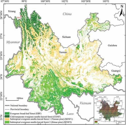
Yunnan Province lies in the southwestern part of China and has a total area of approximately 39.4 × 10⁴ km² (http://yn.gov.cn/yngk/). It borders Myanmar at its western and southwestern borders and Laos and Vietnam to the south and southeast (Figure 1). The topography is diverse, mainly containing mountainous and plateau landscapes with scattered flat valley basins. The elevations in the study area range from approximately 76 m in the southern part to 6740 m (the summit of Meili Mountain) in the northwestern region (Zeng 2018). Because of its unique topographical situation, Yunnan Province exhibits various mountainous topoclimates, ranging from lowland tropical and subtropical climates in the southern region to highland climates in the northwest plateau, both of which are collectively influenced by the southeast and southwest Asian monsoons. Accordingly, the region displays a varied forest composition and pronounced vertical zonation in which subalpine and montane temperate forests are present at higher elevations in the northwestern region, while tropical rainforests and subtropical forests exist at lower elevations in the southern area (Li and Walker 1986). Evergreen broad-leaved forests (EBFs) dominate the lowlands in the southern portion of the province (Zhu 2021), subtropical evergreen needle-leaved forests mainly composed of Yunnan pine (Pinus yunnanensis) (SENF1) or Simao pine (Pinus kesiya) and Masson pine (Pinus massoniana) (SENF2) are present in central and southern Yunnan (Su et al. 2015; Zeng 2018), and cold-temperate evergreen needle-leaved forests (CENFs) are present in northwestern Yunnan (Jiang 1980; Zeng 2018) (Figure 1).

Figure 1. Spatial distribution of four forest types in Yunnan Province. The topography and footprints of the 27 Landsat scenes covering the study area are also presented in the inset (a). The shapefile data of the national and provincial regions were provided by the Standard Map Service System of the Ministry of Natural Resources of the People’s Republic of China website (http://bzdt.ch.mnr.gov.cn/), and the forest distribution data were procured from the 1990 vegetation vector database of Yunnan Province.

3. Data and methods

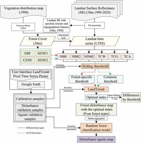
In this study, we aimed to detect forest disturbances and attribute the causal agents at the yearly time step using the LandTrendr algorithm and composite images of yearly cloud-free Landsat observations. The data processing and analysis procedures (Figure 2) mainly involved (1) producing initial forest cover data at the beginning of the study period (in 1990), (2) examining the performances of six SIs in detecting forest disturbances in four broad forest types with the LandTrendr algorithm, (3) investigating the effectiveness of two threshold methods (i.e. a forest-specific threshold and a common threshold) in determining forest disturbances with the best-performing SI, (4) mapping forest disturbances with the best-performing SI and threshold method, and (5) classifying the causal agents (including wildfire, logging and commodity-driven plantation) of forest disturbances using an RF classifier.

Figure 2. Flowchart of the data processing and analysis procedures followed in this study. EBF, CENF, SENF1 and SENF2 are abbreviations representing evergreen broad-leaved forests, cold-temperate evergreen needle-leaved forests, and subtropical evergreen needle-leaved forests dominated by Yunnan pine and by Simao pine, respectively. NBR, NBR2, NDMI, TCA, TCW and TCG denote the normalized burn ratio, normalized burn ratio 2, normalized difference moisture index, tasseled cap angle, tasseled cap wetness and tasseled cap greenness, respectively. The User Interface (UI) LandTrendr Pixel Time Series Plotter was provided by the Oregon State University eMapR Laboratory and Google Earth Engine (GEE) website: https://emaprlab.users.earthengine.app/view/lt-gee-pixel-time-series.

3.1 Data sources and preprocessing

3.1.1 Reference data

Four groups of reference samples (Table S4) were collected via visual interpretation of fine spatial-resolution imagery from Google Earth^TM individually or by jointly combining the temporal trajectories of SIs derived by the user interface of LandTrendr Pixel Time Series Plotter (https://emaprlab.users.earthengine.app/view/lt-geepixel-time-series). The first group included a total of 3134 reference samples of ENF types, of which 570 samples were obtained from CENF sites, 2126 samples represented SENF1 sites and 438 samples were derived from SENF2 sites. These reference samples were collected using a stratified random sampling method and were randomly divided into the training samples (70%) and the validation samples (30%). The training samples were applied to train the RF classifier on the Google Earth Engine (GEE) platform to classify the coarse ENF class extracted from the 1990 vegetation vector database of Yunnan Province into the CENF, SENF1 and SENF2 types, whereas the validation samples were used to calculate the classification accuracies. The second group of reference samples, which consisted of 1819 and 2100 individual validation samples separately representing the disturbance and non-disturbance classes, was used to compute the forest disturbance mapping accuracy. These disturbance and non-disturbance validation samples were randomly and separately extracted from the pixels with an obvious monotonically decreasing spectral trajectory and those with a constant spectral trajectory in the forested areas. Each yearly validation sample obtained for the disturbance and non-disturbance classes contained more than 10 validation samples. The third group contained a total of 800 reference samples (referred to as calibration samples), consisting of 100 disturbance and 100 non-disturbance samples for each forest type; this group was used to examine the optimal disturbance threshold value using the sliding threshold method (Grogan et al. 2015; Tang et al. 2019). These disturbance and non-disturbance samples were derived from the second group of reference samples using a stratified random sampling method. The fourth group of reference samples consisted of 1708 patch samples representing disturbance attribution agents; among the samples, 632 represented wildfire disturbances, 345 characterized logging, and 731 represented commodity-driven plantation. These patch samples were randomly selected from the disturbance samples and then labelled through visual interpretation of high-resolution images; subsequently, 70% of them were extracted as the training set, and the remaining 30% were used as the validation set using a stratified random sampling method. We used the training set to construct the RF agent attribution model, and the validation set to calculate the mapping accuracy of the forest disturbance attribution agents.

3.1.2 Generation of the baseline forest map

The initial forest cover information was used as the basis for detecting forest disturbances. To gain better understanding of the distribution of forest types, we first extracted a raw baseline forest map composed of evergreen broad- and needle-leaved forests from the 1990 vegetation vector database of Yunnan Province. For ENF classification, we stacked the clear Landsat-5 Thematic Mapper (TM) images in 1990 and associated texture information, the topography variables (elevation, aspect, slope and relief shading) generated from the 30-m-resolution Shuttle Radar Topography Mission (SRTM) digital elevation model (DEM), the multispectral bands and derivations (such as the NDVI, enhanced vegetation index (EVI), and tasseled cap brightness (TCB), wetness (TCW), and greenness (TCG)). The overall accuracy for classifying the ENF types was 82.42%. The resultant ENF classification map was merged with the EBF layer extracted from the baseline forest map to yield a final baseline forest map that included the following four forest types: EBF, CENF, SENF1 and SENF2 (Figure 1).

3.1.3 Processing of LTS

Yunnan Province is fully covered by 27 Landsat scenes in the Landsat Worldwide Referencing System (WRS-2) (see Figure 1a). All precision Level-1-Terrain-Corrected (L1T) surface reflectance imagery from Landsat 5/7/8 corresponding to these scenes during the predefined nongrowing seasons (November-December of one year and January-April of the next year) from 1990 to 2020 were extracted with the GEE cloud-computing platform (Gorelick et al. 2017). To produce yearly time series stacks of cloud-free Landsat images from all available clear observations, pixels that were covered by clouds, cloud shadows or snow in each image were screened using the CFMask algorithm (Foga et al. 2017); then, the reflectance harmonization function developed by Roy et al. (2016) was applied to reduce radiometric differences and improve the temporal consistency of surface reflectance between Landsat sensors. Subsequently, yearly cloud-free composite images were generated from clear observations using a best available pixel method (White et al. 2014).

3.2 Forest disturbance detection with forest-specific and common thresholds

The LandTrendr temporal segmentation algorithm (Kennedy, Yang, and Cohen 2010; Kennedy et al. 2018) was adopted in this study to capture and detect both abrupt and gradual time series disturbances with the analyzed SIs based on the GEE platform. The LandTrendr algorithm decomposes the SI time series of each pixel into a series of linear segments to produce a fitted spectral trajectory and segment characteristics. In this study, the LandTrendr process was individually conducted in four forest types to investigate the effectiveness of six SIs, and thereby, the performances of the forest-specific thresholds and a common threshold were examined with the best-performing SI.

3.3 SIs and magnitude threshold calibration

The sensitivities of different bands or SIs to forest canopy structure changes are important for forest disturbance detection because the different spectral bands or indices have varied capabilities for accurately detecting disturbance signals (Kennedy, Yang, and Cohen 2010). In this study, six SIs were computed using the time series of each forest type: NBR, NBR2, NDMI, TCG, TCW and TCA (Table S1).

We performed forest disturbance detection to determine the optimal threshold of disturbance magnitude by applying the LandTrendr algorithm to the six SIs. During this process, 200 calibration samples for each forest type (i.e. 100 for disturbance and 100 for non-disturbance) were used to compute the accuracies of forest disturbance mapping. The optimal disturbance magnitude thresholds of these six SIs for the four forest types were obtained individually using a sliding threshold method . For each of the six SIs, the average and standard deviation of the disturbed samples were calculated; then, relatively continuous user’s accuracy (UA) and producer’s accuracy (PA) curves for the class of disturbed forest were drawn at a step length of 0.1 times the standard deviation. The optimal disturbance magnitude thresholds were defined at the point where the differences between the PA and UA were balanced (Eq. 1)(1) $min\left\{\left|\left|\frac{\mathrm{P}\mathrm{A}\left(\mathrm{\Delta }\mathrm{I}\mathrm{n}\mathrm{d}\mathrm{e}{\mathrm{x}}_{i+1}\right)-\mathrm{P}\mathrm{A}\left(\mathrm{\Delta }\mathrm{I}\mathrm{n}\mathrm{d}\mathrm{e}{\mathrm{x}}_i\right)}{d\left(\mathrm{\Delta }\mathrm{I}\mathrm{n}\mathrm{d}\mathrm{e}\mathrm{x}\right)}\right|-\left|\frac{\mathrm{U}\mathrm{A}\left(\mathrm{\Delta }\mathrm{I}\mathrm{n}\mathrm{d}\mathrm{e}{\mathrm{x}}_{i+1}\right)-\mathrm{U}\mathrm{A}\left(\mathrm{\Delta }\mathrm{I}\mathrm{n}\mathrm{d}\mathrm{e}{\mathrm{x}}_i\right)}{d\left(\mathrm{\Delta }\mathrm{I}\mathrm{n}\mathrm{d}\mathrm{e}\mathrm{x}\right)}\right|\right|\right\}$(1) . Additionally, forest-specific thresholds for individual forest types and a common threshold for all forest types were separately extracted. The accuracies obtained herein were used only to determine the optimal threshold but cannot explain the final disturbance detection accuracy.

(1) $min\left\{\left|\left|\frac{\mathrm{P}\mathrm{A}\left(\mathrm{\Delta }\mathrm{I}\mathrm{n}\mathrm{d}\mathrm{e}{\mathrm{x}}_{i+1}\right)-\mathrm{P}\mathrm{A}\left(\mathrm{\Delta }\mathrm{I}\mathrm{n}\mathrm{d}\mathrm{e}{\mathrm{x}}_i\right)}{d\left(\mathrm{\Delta }\mathrm{I}\mathrm{n}\mathrm{d}\mathrm{e}\mathrm{x}\right)}\right|-\left|\frac{\mathrm{U}\mathrm{A}\left(\mathrm{\Delta }\mathrm{I}\mathrm{n}\mathrm{d}\mathrm{e}{\mathrm{x}}_{i+1}\right)-\mathrm{U}\mathrm{A}\left(\mathrm{\Delta }\mathrm{I}\mathrm{n}\mathrm{d}\mathrm{e}{\mathrm{x}}_i\right)}{d\left(\mathrm{\Delta }\mathrm{I}\mathrm{n}\mathrm{d}\mathrm{e}\mathrm{x}\right)}\right|\right|\right\}$(1)

$\left(i=1,2,3\cdots ,50\right)$

where $\mathrm{\Delta }$ Index refers to the different SIs; d is the standard deviation; i is the number of threshold step length; PA and UA represent producer’s accuracy and user’s accuracy, respectively.

3.4 Forest disturbance agent attribution

By assessing past surveys regarding the driving factors of forest disturbances in the study area, three major disturbance agents (wildfire, logging and commodity-driven plantations) were selected for consideration in this study. Wildfire, logging, and commodity-driven plantations are characterized by forest stand modifications from large-scale burning, permanent removal of forests, and temporary removal of natural forests and the subsequent substitution by plantations of rubber or tea trees, respectively. The adjacent disturbed pixels within a 3 × 3 pixel window in the same year were aggregated into disturbance patches for the subsequent disturbance agent attribution process.

Five groups of comprehensive predictor variables, including patch-based temporal characteristics, LandTrendr-derived spectral properties (e.g. the pre- and post-disturbance spectral values), disturbance segmentation characteristics, topographic metrics and geometric attributes, and the associated statistical features were used in this study (Table S2). Multicollinearity analyses were iteratively performed to remove predictor variables with variance inflation factor (VIF) thresholds above 10 (Hermosilla et al. 2015). In total, 17 predictor variables were selected from the 43 candidate predictor variables (Table S3).

As has been suggested by Hermosilla et al. (2015) and Kennedy et al. (2015), an RF model with 500 trees and 17 selected predictor variables was used herein to classify the disturbance agents (i.e. wildfire, logging and commodity-driven plantation). The model outputs were defined by majority votes of the trees, derived by random selection of training sample subsets and predictors at each node. The number of predictors in the subsets randomly selected at each node was set to $\sqrt{17}$ (the square root of the count size of all selected predictors) in this study.

3.5 Accuracy assessment

The mapping accuracies of forest disturbance derived for the four forest types with six SIs were evaluated with the second group of reference samples (section 3.1.1). The overall accuracy (OA), UA and PA were computed based on the two kinds of confusion matrices, namely, the traditional confusion matrix and the error-adjusted estimated matrix developed by Olofsson et al. (2013, 2014). The traditional confusion matrix refers to the error matrix regarding sample counts, whereas the error-adjusted estimated matrix employs the area derived from pixel counting to adjust the error matrix. In the error-adjusted estimation process, the accuracy measure variances were computed using the 5% significance levels of the disturbed and undisturbed forest areas.

The disturbance agent attribution mapping accuracy derived using the RF model was assessed using a traditional confusion matrix based on the validation set extracted from the fourth group of reference samples, whereas the error-adjusted estimated matrix was used to calculate the mapping accuracy of forest disturbance detection among six SIs between two threshold methods.

3.6 Statistical analyses

A nonparametric Mann–Whitney U test (Hollander et al. 2015) was used to test the statistical significance of the disturbance areas generated from the two threshold methods at the 95% (α = 0.05) and 99% (α = 0.01) confidence intervals. We applied the Mann-Kendall (MK) test to detect whether the trends in annual disturbed forest areas were statistically significant at the 95% (α = 0.05) and 99% (α = 0.01) confidence intervals; meanwhile, changes in the trend magnitude were computed using Sen’s slope estimator. A change point analysis based on the MK test was also conducted to determine whether abrupt change points existed in the annual time series of disturbed forest areas in different forest types. Analysis of variance (ANOVA) was used to determine whether a significant difference existed among the six SIs and among the forest types (Sthle and Wold 1989). The above mentioned statistical analyses were performed in the R language.

4. Results

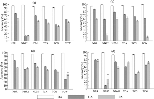
4.1 Differences in disturbance detection accuracy among the six SIs

As shown in Figure 3, the OAs, PAs and UAs derived when mapping forest disturbances with the forest-specific disturbance magnitude threshold method (Table S5) varied by forest type and SI. The ANOVA test results indicated that the variations in OA, UA and PA with SI and forest type were statistically significant at a significance level of 0.05. Among the examined SIs, the NBR exhibited higher OAs and more balanced UAs and PAs than the other SIs; OAs of 94.47 ± 0.25% for EBF, 93.45 ± 0.38% for CENF, 93.04 ± 0.17% for SENF1, and 96.09 ± 0.28% for SENF2 were obtained. The NDMI and TCA also produced relatively high OAs, PAs and UAs, exhibiting OAs ranging from 92.84%±0.28% for EBF to 96.09 ± 0.28% for SENF2. The TCG, TCW and NBR2 exhibited relatively low OAs, PAs and UAs. In particular, NBR2 yielded the lowest PAs and UAs for the analyzed forest types, excluding SENF1. The TCW had higher accuracies for the EBF and SENF2 forest types than for the CENF and SENF1 forest types, whereas the TCG presented the opposite behavior.

Figure 3. OAs, UAs, and PAs reflect the forest disturbance detection abilities of six disturbance indices (SIs; NBR, NBR2, NDMI, TCW, TCA, and TCG) considering forest-specific disturbance magnitude thresholds for the four forest types: (a) EBF, (b) CENF, (c) SENF1, and (d) SENF2.

4.2 Disturbance detection accuracy differences between the two threshold methods

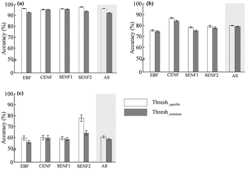
Figure 4 demonstrates that the forest-specific threshold method produced higher accuracies (OAs, PAs and UAs) than the common threshold method when used to detect NBR-based forest disturbances. The improvements in the OA, UA and PA ranged from 0.14% in CENF to 3.92% in SENF2, from 0.88% in EBF to 3.01% in SENF1, and from 0.25% in CENF to 13.47% in SENF2 respectively. Among the four forest types, larger improvements were observed in the OA and PA for EBF (3.59% and 3.78%) and SENF2 (3.92% and 13.47%) and the UA for SENF1 (3.01%) and CENF (2.70%). Compared with the common threshold method, the forest-specific threshold method produced higher OA, UA and PA, with increases of 3.88%, 0.75% and 2.07%, respectively.

Figure 4. Comparison of the NBR-based disturbance detection accuracies obtained using a common disturbance threshold and forest-specific disturbance thresholds corresponding to four individual forest types: (a) OA, (b) UA and (c) PA. Thresh__specific and Thresh__common represent the forest-specific disturbance magnitude thresholds corresponding to four individual forest types and the common disturbance threshold applied to all forest types, respectively.

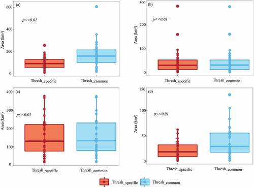
As illustrated in Figure 5, the difference in the derived annual disturbed forest areas between the forest-specific and common threshold methods was statistically significant. The common threshold method produced larger median annual disturbed areas than the forest-specific threshold method, especially for the EBF and SENF2 sites (Figure 5a,). By comparison, the interannual variations in the annual disturbed forest areas mapped using the forest-specific threshold method were smaller than those derived using the common threshold method, with the exception of the CENF regions. In addition, the accuracy assessment of yearly forest disturbances demonstrated that the medians of PAs and UAs for the forest-specific threshold method were 93.73% and 94.48%, respectively, which were considerably higher than those for the common threshold method (92.20% and 92.04%) (Tables S6 and S7).

Figure 5. Boxplots of the annual disturbed forest areas mapped using the NBR-based forest disturbance detection process with the forest-specific disturbance magnitude threshold method and the common disturbance magnitude threshold method. The solid points represent the mapped disturbance area of each year. (a) EBF, (b) CENF, (c) SENF1, and (d) SENF2. The difference in the disturbed areas between Thresh__specific and Thresh__common was statistically tested with a Mann–Whitney U test at the 95% (α = 0.05) and 99% (α = 0.01) significance levels. Thresh__specific and Thresh__common represent the forest-specific disturbance thresholds derived for four individual forest types and the common disturbance threshold applied for all forest types, respectively.

4.3 Mapping forest disturbances and agent attributions in Yunnan

4.3.1 Forest disturbances in different forest types

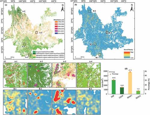
As depicted in Figure 6(a), the spatial distribution of forest disturbances reflected dispersed disturbances in eastern Yunnan but highly clustered disturbances in the northwestern, southern and central parts of Yunnan. Forest disturbances were widespread at the forest border regions. Disturbed forest patches with relatively large areas and irregular shapes occurred predominantly in the CENF and SENF1 regions (A-2 and A-3), while disturbances associated with smaller areas and more geometrical shapes mainly occurred in the EBF and SENF2 regions (A-1 and A-4). Figure 6(b) shows that relatively concentrated forest disturbance hot spots were observed in northwestern, southern and central Yunnan; in these regions, the disturbance patches were relatively clustered (Figure 6(a)). The statistical results shown in Figure 6(d) further demonstrate that the total mapped forest area disturbed between 1990 and 2020 amounted to 9831.48 km², accounting for approximately 5.31% of the original forest area in 1990 across Yunnan Province. The SENF1, EBF, CENF and SENF2 forest types individually contributed approximately 47.71% (4690.37 km²), 30.52% (3000.09 km²), 14.62% (1437.65 km²) and 7.15% (703.37 km²) of the total mapped disturbed area, respectively.

Figure 6. The spatial patterns of forest disturbances (a) and hot spots (b) from 1990 to 2020 in Yunnan Province. A-1–A-4 in panel (c) display magnified images of forest disturbances in EBF, CENF, SENF1, and SENF2. B-1–B-4 in panel (c) represent disturbance hot spots in EBF, CENF, SENF1, and SENF2. The mapped forest disturbance areas and areal percentages in the four analyzed forest types are also shown in panel (d).

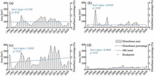
The mapped annual areas and areal percentages of disturbed forests varied substantially among the analyzed forest types (Figure 7). Among the four forest types investigated, EBF and SENF1 contributed more disturbed areas than CENF or SENF2 in most years, excluding the two years of 1994 and 2000, in which larger disturbed areas were distributed in CENF regions. The median values of the annual disturbed areas were 93.51 km² in EBF, 32.33 km² in CENF, 130.54 km² in SENF1 and 19.26 km² in SENF2, with corresponding interquartile ranges of 71.73 km², 40.32 km², 144.90 km² and 22.93 km², respectively (Figures 5 and 7). The mapped annual disturbed areas in the four forest types exhibited upwards trends (Figures 7 (a–7)), but this upwards trend was statistically significant only in SENF2, in which a change point could be identified in 2001 (Figure 7(d)).

Figure 7. Annual mapped areas and areal percentages of disturbed forests from 1990 to 2020 in the four forest types: (a) EBF, (b) CENF, (c) SENF1, and (d) SENF2.

4.3.2 Agent contribution of forest disturbances in different forest types

The OA of attributing the causal agents of disturbed patches of forest was 82.49% (Table 1). Among the three predefined causal agents, wildfire agents presented the highest PA (88.59%) and UA (85.19%), and logging agents had a higher PA and lower UA than commodity-driven plantation agents.

Table 1. Attribution accuracies of the analyzed disturbance agents.

Agent class	PA (%)	UA (%)	OA (%)
Wildfire	88.59	85.19	82.49
Logging	82.70	73.80
Commodity-driven plantations	71.39	80.66

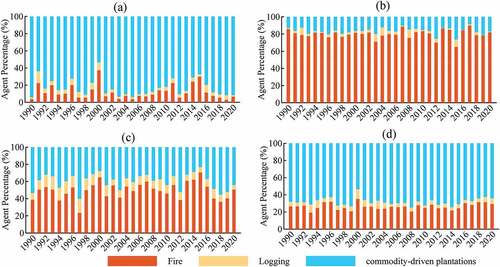
As illustrated in Figure 8(a), wildfire-induced forest disturbances prevailed in the northwestern and central parts of Yunnan, whereas commodity-driven plantation-caused forest disturbances mainly occurred in southern and southeastern Yunnan. The mapped forest patch areas disturbed by wildfires, logging and commodity-driven plantations were 4086.93 km², 673.86 km² and 5070.69 km², respectively, accounting for 41.57%, 6.58% and 51.58% of the total mapped disturbed area (Figure 8(b)). Figure 9 further shows that the annual mapped areas and areal percentages of disturbed forest patches resulting from wildfire, logging and commodity-driven plantation agents varied substantially among the analyzed forest types. Commodity-driven plantation agents were the predominant causal factor inducing forest disturbances in EBF and SENF2, with average areal percentages of 83.42% and 68.34%, respectively, followed by wildfire agents, with corresponding average areal percentages of 11.87% and 26.14% (Figures 9(a,d)). In contrast, wildfire agents were the leading contributing factor causing forest disturbances in CENF and SENF1, with average areal percentages of 79.97% and 49.45%, respectively, followed by commodity-driven plantation agents, with corresponding average areal percentages of 16.59% and 39.96% (Figures 9(b,c)). The areal percentages of disturbed forests contributed by logging agents were small, with average values of 3.43–10.59% (Figure 9).

Figure 8. Spatial distribution of forest disturbance agent classes (a) and the areas and percentages of forests affected by different causal agents (b) in Yunnan Province.

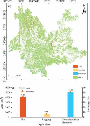
Figure 9. Areal percentages of disturbed forest patches caused by the three analyzed disturbance agents (i.e. wildfire, logging and commodity-driven plantation agents) between 1990 and 2020 in the four studied forest types: (a) EBF, (b) CENF, (c) SENF1, and (d) SENF2.

5. Discussion

5.1 Performance of the SIs in forest disturbance mapping

The six investigated SIs performed differently in response to disturbances in different forest types. The NBR exhibited consistently better performances in all four forest types compared to the other five SIs, thus indicating that the NBR has promising potential for detecting forest disturbances in different forest types in the study area. Although NBR has been reported to be suitable for forest disturbance mapping in existing studies (Kennedy, Yang, and Cohen 2010; Smith et al. 2019; Meng et al. 2021) due to its high sensitivity to chlorophyll, leaf and soil wetness and canopy cover closure and its associated ability to discriminate between healthy and damaged forests (Howard et al. 2002), the outperformance of the NBR when mapping forest disturbances in multiple forest types over large areas remains unquantified based on our knowledge. This study suggests that the PAs and UAs obtained regarding the NBR performance when mapping disturbances in four forest types were 1.81–5.06% and 0.39–1.64% higher, respectively, than those of the second-best-performing SIs (excluding the NDMI results in SENF1).

The NDMI had a consistently good performance and was second only to the NBR. The SIs of the NBR and NDMI similarly use the reflectance disparity between the near-infrared (NIR) and shortwave infrared (SWIR) wavelengths, and this metric is suitable for detecting forest disturbances (DeVries et al. 2015a; Cohen et al. 2018). Although the NDMI has demonstrated effective performance when detecting forest disturbances in previous studies (DeVries et al. 2015a; Ochtyra, Marcinkowska-Ochtyra, and Raczko 2020), the NBR considerably outperformed the NDMI by substituting SWIR1 with SWIR2 (Table S1) in most cases. SWIR bands and their derivatives are sensitive to forest canopy moisture and structure and thus have exhibited more responsiveness to external disturbance (Grogan et al. 2016). The performances of the SIs of the TCA, TCW, TCG and NBR2 varied substantially among the different forest types. As a combination of TCB and TCG, TCA performed better and was less dependent on forest types than the remaining three SIs but was still inferior to the NBR and NDMI. Although the TCW has been suggested as the optimal index for use in change analyses of diverse forest types by Czerwinski, King, and Mitchell (2014) and Grogan et al. (2015), this SI performed poorly in the SENF1 regions in our study. The performances of the NBR2 and TCG SIs were highly dependent on the forest types; these two SIs performed fairly well for CENF and SENF1 but very poorly for EBF and SENF2, as they failed to effectively capture the change signals caused by different disturbances (Smith et al. 2019).

These findings highlight the various abilities of different SIs to detect forest disturbance in different forest types. The NBR, NDMI and TCA SIs exhibited reliably good performance for all forest types, whereas the performances of the remaining three SIs (NBR2, TCW and TCG) were heavily dependent on the forest type. Although some SIs were shown to be consistently outperformed in this study, a comprehensive quantitative evaluation of the performances of different SIs is still recommended when detecting forest disturbances in specific forest types, especially for areas comprising various forest types.

5.2 Forest-specific thresholds versus a single common threshold for detecting forest disturbances

Our results showed that the forest-specific disturbance magnitude threshold method yielded higher forest disturbance mapping accuracies than the common single threshold method; the former method resulted in OA, UA and PA increases of 0.14–3.92%, 0.88–3.01% and 0.25–13.47%, respectively, compared to the latter method (Figure 4). Accordingly, higher annual disturbed forest areas and wider interannual fluctuations were observed under the common threshold method, indicating that the forest-specific threshold method can effectively remove the falsely disturbed pixels detected by the common threshold method and subsequently lead to an increased forest disturbance mapping accuracy (Tables S6 and S7). These findings emphasize the great importance of defining the thresholds for specific forest types in areas with varied forest types. Different forest types have different canopy structures and phenologies and then exhibit unique trajectories of SIs in response to external disturbances; therefore, the disturbance magnitudes reflected by the SIs are necessarily forest type-specific. Thus, the use of a single common disturbance magnitude threshold ignores the different spectral and phenological features among different forest types, thus leading to disturbance overestimations (Ochtyra, Marcinkowska-Ochtyra, and Raczko 2020). The change magnitudes of SIs resulting from different disturbance agents are determined by the differences between pre- and post-disturbance observational SIs, which were less related to disturbance agents. Thus, the optimal thresholds to identify forest disturbance varied substantially with forest types rather than disturbance agents. In the cases where pre- and post-disturbance observational SIs of different forest types are similar, the specific magnitude thresholds depend heavily on the disturbance agents. It can be inferred that the disturbance detection improve best when applying specific magnitude thresholds in different forest types with the same disturbance agents. Although previous studies also emphasized the importance of optimizing thresholds of spectral change magnitude when detecting forest disturbance (DeVries et al. 2015b; Hermosilla et al. 2015; Schroeder et al. 2017), the dependence of the change magnitude thresholds of SIs for forest disturbance detection on specific forest types was not revealed. Additionally, the optimal threshold magnitudes generated by maximizing accuracy metrics are often region-dependent and forest type-specific (DeVries et al. 2015a, 2015b; Hamunyela, Verbesselt, and Herold 2016). Chen et al. (2021) confirmed that applying only a single optimal metric alone to all forest types produced a lower forest degradation detection OA compared to that obtained when using different optimal metrics for different forest types. Grogan et al. (2016) suggested that forest disturbance mapping can be substantially improved by accounting for forest type, and forest type-specific models limited the error distribution among various types of forest. On the contray, recent studies demonstrated that classifying an ensemble of multispectral bands and indices could provide more accurate forest disturbance results using a supervised classifier (Cohen et al. 2018; Shimizu et al. 2019). In comparison, the forest-specific threshold method proposed here also achieved a comparable disturbance detection accuracy. However, the subtle or low-magnitude disturbances are difficult to be captured and might be missed in the ensemble methods (De Marzo et al. 2021), thus a target magnitude threshold was recommended for improving the disturbance results (Cohen et al. 2018). Therefore, this study represents the first investigation into the effects of applying forest type-specific disturbance magnitude thresholds on the performance of the LandTrendr algorithm in forest disturbance detection and demonstrates the value of discriminating forest types when mapping forest disturbance.

5.3 Variations in forest disturbance and the attribution to forest types

The high accuracies derived when mapping forest disturbances and agent attributions using yearly LTS indicated the robust performance of the LandTrendr algorithm and RF classifier when the NBR SI and forest-specific disturbance magnitude threshold method were applied. The disturbance detection results obtained for the four forest types exhibited consistently high OAs ranging from 93.04 ± 0.17% to 96.09 ± 0.28%; these values are higher than 87.5% of the outcomes derived by Nguyen et al. (2018) in Australia and are slightly inferior to the values of 97.70 ± 0.06% obtained in the Hengduan Mountains region (Li et al. 2021). The OA (82.49%) of the forest disturbance agent attribution was higher than 80.7% of the outcomes obtained in Australia (Nguyen et al. 2018) but lower than 84.7% of the values derived in Myanmar (Shimizu et al. 2017). Compared to the previous studies mentioned above, this study provided mapping accuracies for four typical forest types in China’s Yunnan Province; this study region is characterized by highly heterogeneous and diverse forest landscapes, which can lead to accuracy losses when mapping forest disturbances and agent attributions.

The mapped total disturbed area, including all four forest types across all of Yunnan Province from 1990–2020, was 9831.48 km², approximately 5.31% of the total forested area in 1990. This forest disturbance rate was higher than the rate of 2.31% obtained in the Hengduan Mountains region (Li et al. 2021) and the global forest loss rate of 4.2% (FAO 2020) but considerably lower than the forest change rate (17%) measured in the humid tropics over the same study period (Vancutsem et al. 2021).

Our results illustrated distinct forest disturbance and agent attribution patterns in four forest types in Yunnan. Approximately 79% of the forest disturbances were located in the SENF1 and EBF distribution areas. Across all forest types in Yunnan, wildfires and commodity-driven plantations were the two overwhelmingly predominant disturbance agents; together, these agents contributed approximately 93.15% to the total mapped disturbed area from 1990–2020. In particular, SENF1 (dominated by Yunnan pine) and CENF were mainly distributed in northwestern and central Yunnan and were found to be wildfire-prone, as wildfires are beneficial to species persistence and ecosystem sustainability (Su et al. 2015; Pausas et al. 2021). The EBF and SENF2 (dominated by Simao pine) regions located in southern Yunnan were mainly affected by commodity-driven plantation-dominated forest disturbances, mainly driven by the extensive expansion of rubber and other cash crops (Li et al. 2007; Liao et al. 2014; Liu et al. 2014). Widespread commodity-driven plantation expansion also led to a significant increasing trend in the annual mapped disturbed area, contributing a breakpoint in 2001 in the SENF2 regions. In comparison, logging had a smaller contribution to forest disturbances, which may have been associated with the strict implementation of China’s Natural Forest Conservation Program (NFCP) launched in the late 1990s (Yang 2017). Furthermore, some small-scale logging disturbances (e.g. selective logging) cannot be accurately captured or attributed because of the medium spatial resolution of Landsat images and the lack of inclusion of disturbance threshold metrics related to forest degradation (Chen et al. 2021). Overall, it can be concluded that the forest disturbance of Yunnan Province was mainly due to wildfires and commodity-driven plantations over the past three decades. Although soundly accurate 31-year spatiotemporal forest disturbance and agent attribution patterns across the vast Yunnan Province were presented in association with forest types, the 1990 forest type baseline map was based on optical images, and its accuracy was not sufficiently high due to the frequent occurrence of mixed pixels in heterogeneous forests and the lack of adequate retrospective reference samples derived from field inventory data or high-resolution images (Griffiths et al. 2014). Moreover, this study investigated only three subjectively defined proximate causal agents of forest disturbances. The underlying natural and anthropogenic driving forces of these disturbances, such as forest management policies and shifts in socioeconomic development, remain unexplored. Furthermore, forest degradation processes characterized by partial canopy cover or structural losses were not considered in the present study (Chen et al. 2021). In future work, the fusion of Landsat data with radar or light detection and ranging (LIDAR) data should be explored to conduct more comprehensive forest change monitoring, especially forest changes associated with degradation (Hirschmugl et al. 2020).

6. Conclusion

Comprehensive forest disturbance information collected over long time periods is important for forest management. In this study, we explored and compared the performances of six SIs (i.e. NBR, NBR2, NDMI, TCA, TCW, and TCG) and two disturbance magnitude threshold methods (i.e. forest-specific and common thresholds) when mapping forest disturbances with a LandTrendr algorithm based on LTS data collected in four forest types (i.e. EBF, CENF, SENF1, and SENF2 forests) across Yunnan Province, China, from 1990 to 2020. The results highlighted the importance of the optimal selection of SIs and disturbance magnitude thresholds for detecting forest disturbances in large areas comprising various forest types. Among the six SIs, the NBR outperformed the remaining five SIs, yielding consistently higher mapping accuracies than the other SIs for all four forest types. We also found that the use of a forest-specific threshold method significantly improved the forest disturbance detection accuracies in the four analyzed forest types, with increased OA, UA and PA of 0.14–3.92%, 0.88–3.01% and 0.25–13.47%, respectively. Furthermore, the spatial and temporal forest disturbance patterns were demonstrated in-depth in the four different analyzed forest types. The total mapped disturbed forest area reached 9831.48 km² (5.31%) in Yunnan Province from 1990 to 2020, and approximately 79% of this area occurred in the SENF1 and EBF distribution areas. Spatially, forest disturbances were more dispersed in eastern Yunnan but more clustered in northwestern, southern and central Yunnan. Wildfires and commodity-driven plantations were the two leading causal agents of forest disturbances, contributing approximately 93.15% of the total disturbed forest area. Forest disturbances in CENF and SENF2 were dominated by wildfires, while disturbances in EBF and SENF2 were dominated by commodity-driven plantations. Therefore, over the last three decades, Yunnan Province has been a disturbance region of wildfire- and commodity-driven plantation-dominated forest disturbances. In further work, more comprehensive forest disturbance and forest degradation surveys could be conducted by integrating optical and microwave satellite data, and the underlying causal factors and driving mechanisms of forest changes could be further uncovered at the regional scale.

Acknowledgements

This research was jointly supported by the Second Tibetan Plateau Scientific Expedition and Research Program (STEP) (Grant No. 2019QZKK0402), the National Natural Science Foundation of China (Grant No. 41971239), Scientific Research Foundation of Yunnan Provincial Education Department (Grant No. 2022Y061), and the programme for the provincial innovative team of the climate change study of the Greater Mekong Subregion (Grant No. 2019HC027).

Disclosure statement

No potential conflict of interest was reported by the author(s).

Data availability statement

All the Landsat time series data in this study are openly available from the Google Earth Engine (GEE) platform cloud-computing platform (https://developers.google.com/earth-engine/datasets/catalog/landsat).

Supplementary material

Supplemental data for this article can be accessed online at https://doi.org/10.1080/15481603.2022.2127459.

Additional information

Funding

This work was supported by the Second Tibetan Plateau Scientific Expedition and Research Program (STEP) [2019QZKK0402]; National Natural Science Foundation of China [41971239]; Programme for the provincial innovative team of the climate change study of the Greater Mekong Subregion [2019HC027]; Scientific Research Foundation of Yunnan Provincial Education Department [2022Y061].

References

- Avitabile, V., A. Baccini, M. A. Friedl, and C. Schmullius. 2012. “Capabilities and Limitations of Landsat and Land Cover Data for Aboveground Woody Biomass Estimation of Uganda.” Remote Sensing of Environment 117: 366–380. doi:10.1016/j.rse.2011.10.012.
- Cai, W., C. Yang, X. Wang, C. Wu, L. Larrieu, C. Lopez-Vaamonde, Q. Wen, and D. W. Yu. 2021. “The Ecological Impact of pest-induced Tree Dieback on Insect Biodiversity in Yunnan Pine Plantations, China.” Forest Ecology and Management 491: 119173. doi:10.1016/j.foreco.2021.119173.
- Chen, S., C. E. Woodcock, E. L. Bullock, P. Arévalo, P. Torchinava, S. Peng, and P. Olofsson. 2021. “Monitoring Temperate Forest Degradation on Google Earth Engine Using Landsat Time Series Analysis.” Remote Sensing of Environment 265: 112648. doi:10.1016/j.rse.2021.112648.
- Cohen, W. B., S. P. Healey, Z. Yang, S. V. Stehman, C. K. Brewer, E. B. Brooks, N. Gorelick, et al. 2017. “How Similar are Forest Disturbance Maps Derived from Different Landsat Time Series Algorithms?” Forests 8 (4): 98–116. doi:10.3390/f8040098.
- Cohen, W. B., S. P. Healey, Z. Yang, Z. Zhu, and N. Gorelick. 2020. “Diversity of Algorithm and Spectral Band Inputs Improves Landsat Monitoring of Forest Disturbance.” Remote Sensing 12 (10): 1673–1687. doi:10.3390/rs12101673.
- Cohen, W. B., Z. Yang, S. P. Healey, R. E. Kennedy, and N. Gorelick. 2018. “A LandTrendr Multispectral Ensemble for Forest Disturbance Detection.” Remote Sensing of Environment 205: 131–140. doi:10.1016/j.rse.2017.11.015.
- Crist, E. P., and R. C. Cicone. 1984. “A physicallbBased Transformation of Thematic Mapper data—The TM Tasseled Cap.” IEEE Transactions on Geoscience and Remote Sensing GE-22 (3): 256–263. doi:10.1109/TGRS.1984.350619.
- Czerwinski, C. J., D. J. King, and S. W. Mitchell. 2014. “Mapping Forest Growth and Decline in a Temperate Mixed Forest Using Temporal Trend Analysis of Landsat Imagery, 1987–2010.” Remote Sensing of Environment 141: 188–200. doi:10.1016/j.rse.2013.11.006.
- De, M., D. P. Teresa, M. Baumann, E. F. Lambin, I. Gasparri, and T. Kuemmerle. 2021. “Characterizing Forest Disturbances across the Argentine Dry Chaco Based on Landsat Time Series.” International Journal of Applied Earth Observation and Geoinformation 98: 102310. doi:10.1016/j.jag.2021.102310.
- DeVries, B., M. Decuyper, J. Verbesselt, A. Zeileis, M. Herold, and S. Joseph. 2015a. “Tracking disturbance-regrowth Dynamics in Tropical Forests Using Structural Change Detection and Landsat Time Series.” Remote Sensing of Environment 169: 320–334. doi:10.1016/j.rse.2015.08.020.
- DeVries, B., J. Verbesselt, L. Kooistra, and M. Herold. 2015b. “Robust Monitoring of small-scale Forest Disturbances in a Tropical Montane Forest Using Landsat Time Series.” Remote Sensing of Environment 161: 107–121. doi:10.1016/j.rse.2015.02.012.
- FAO. 2020. “Global Forest Resources Assessment 2020: Main Report. Rome.” In.
- Federici, S., F. N. Tubiello, M. Salvatore, H. Jacobs, and J. Schmidhuber. 2015. “New Estimates of CO2 Forest Emissions and Removals: 1990–2015.” Forest Ecology and Management 352: 89–98. doi:10.1016/j.foreco.2015.04.022.
- Finer, M., S. Novoa, M. J. Weisse, R. Petersen, J. Mascaro, T. Souto, F. Stearns, and R. García Martinez. 2018. “Combating Deforestation: From Satellite to Intervention.” Science 360 (6395): 1303–1305. doi:10.1126/science.aat1203.
- Foga, S., P. L. Scaramuzza, S. Guo, Z. Zhu, R. D. Dilley, T. Beckmann, G. L. Schmidt, J. L. Dwyer, M. Joseph Hughes, and B. Laue. 2017. “Cloud Detection Algorithm Comparison and Validation for Operational Landsat Data Products.” Remote Sensing of Environment 194: 379–390. doi:10.1016/j.rse.2017.03.026.
- Gorelick, N., M. Hancher, M. Dixon, S. Ilyushchenko, D. Thau, and R. Moore. 2017. “Google Earth Engine: Planetary-scale Geospatial Analysis for Everyone.” (English) Remote Sensing of Environment 202: 18–27. doi:10.1016/j.rse.2017.06.031.
- Griffiths, P., T. Kuemmerle, M. Baumann, V. C. Radeloff, I. V. Abrudan, J. Lieskovsky, C. Munteanu, K. Ostapowicz, and P. Hostert. 2014. “Forest Disturbances, Forest Recovery, and Changes in Forest Types across the Carpathian Ecoregion from 1985 to 2010 Based on Landsat Image Composites.” Remote Sensing of Environment 151: 72–88. doi:10.1016/j.rse.2013.04.022.
- Grogan, K., D. Pflugmacher, P. Hostert, R. Kennedy, and R. Fensholt. 2015. “Cross-border Forest Disturbance and the Role of Natural Rubber in Mainland Southeast Asia Using Annual Landsat Time Series.” Remote Sensing of Environment 169: 438–453. doi:10.1016/j.rse.2015.03.001.
- Grogan, K., D. Pflugmacher, P. Hostert, J. Verbesselt, and R. Fensholt. 2016. “Mapping Clearances in Tropical Dry Forests Using Breakpoints, Trend, and Seasonal Components from MODIS Time Series: Does Forest Type Matter?” Remote Sensing 8 (8): 657. doi:10.3390/rs8080657.
- Hamunyela, E., J. Verbesselt, and M. Herold. 2016. “Using Spatial Context to Improve Early Detection of Deforestation from Landsat Time Series.” Remote Sensing of Environment 172: 126–138. doi:10.1016/j.rse.2015.11.006.
- Hansen, M. C., P. V. Potapov, R. Moore, M. Hancher, S. A. Turubanova, A. Tyukavina, D. Thau, et al. 2013. “High-resolution Global Maps of 21st-century Forest Cover Change.” Science 342 (6160): 850–853. http://science.sciencemag.org/content/342/6160/850.abstract
- Hermosilla, T., M. A. Wulder, J. C. White, N. C. Coops, and G. W. Hobart. 2015. “Regional Detection, Characterization, and Attribution of Annual Forest Change from 1984 to 2012 Using Landsat-derived time-series Metrics.” Remote Sensing of Environment 170: 121–132. doi:10.1016/j.rse.2015.09.004.
- Hirschmugl, M., J. Deutscher, C. Sobe, A. Bouvet, S. Mermoz, and M. Schardt. 2020. “Use of SAR and Optical Time Series for Tropical Forest Disturbance Mapping.” Remote Sensing 12 (4): 727–755. doi:10.3390/rs12040727.
- Hirschmugl, M., M. Steinegger, H. Gallaun, and M. Schardt. 2014. “Mapping Forest Degradation Due to Selective Logging by Means of Time Series Analysis: Case Studies in Central Africa.” Remote Sensing 6 (1): 756–775. doi:10.3390/rs6010756.
- Hollander, M., D. A. Wolfe, and E. Chicken. 2015. The Two-Sample Location Problem. In Nonparametric Statistical Methods, Third Edition. Wiley Series in Probability and Statistics edited by Hollander, M., Wolfe, D. A., Chicken, E. Hoboken, New Jersey: John Wiley & Sons, Inc. doi:10.1002/9781119196037.ch4.
- Howard, S. M., D. O. Ohlen, R. A. Mckinley, Z. Zhu, and J. Kitchen. 2002. “Historical Fire Severity Mapping from Landsat Data.” In Integrating Remote Sensing at the Global, Regional and Local Scale. ISPRS commission I mid-term symposium in conjunction with Pecora 15/land satellite information IV conference proceedings, November 10-15, 2002, XXXIV Part 1, Denver, Colorado, USA.
- Huang, C., S. N. Goward, J. G. Masek, N. Thomas, Z. Zhu, and J. E. Vogelmann. 2010. “An Automated Approach for Reconstructing Recent Forest Disturbance History Using Dense Landsat Time Series Stacks.” Remote Sensing of Environment 114 (1): 183–198. doi:10.1016/j.rse.2009.08.017.
- Huo, L., L. Boschetti, and A. M. Sparks. 2019. “Object-based Classification of Forest Disturbance Types in the Conterminous United States.” Remote Sensing 11 (5): 477–497. doi:10.3390/rs11050477.
- Jiang, H. 1980. “Distributional Features and Zonal Regularly of Vegetation in Yunnan.” ACTA botanica Yunnannica 2 (1): 22–32. in Chinese with English abstract.
- Kennedy, R. E., Z. Yang, J. Braaten, C. Copass, N. Antonova, C. Jordan, and P. Nelson. 2015. “Attribution of Disturbance Change Agent from Landsat time-series in Support of Habitat Monitoring in the Puget Sound Region, USA.” Remote Sensing of Environment 166: 271–285. doi:10.1016/j.rse.2015.05.005.
- Kennedy, R. E., Z. Yang, and W. B. Cohen. 2010. “Detecting Trends in Forest Disturbance and Recovery Using Yearly Landsat Time Series: 1. LandTrendr — Temporal Segmentation Algorithms.” Remote Sensing of Environment 114 (12): 2897–2910. doi:10.1016/j.rse.2010.07.008.
- Kennedy, R. E., Z. Yang, N. Gorelick, J. Braaten, L. Cavalcante, W. B. Cohen, and S. Healey. 2018. “Implementation of the LandTrendr Algorithm on Google Earth Engine.” Remote Sensing 10 (5): 691. doi:10.3390/rs10050691.
- Kim, D.-H., J. O. Sexton, P. Noojipady, C. Huang, A. Anand, S. Channan, M. Feng, and J. R. Townshend. 2014. “Global, Landsat Based Forest Cover Change from 1990 to 2000.” Remote Sensing of Environment 155: 178–193. doi:10.1016/j.rse.2014.08.017.
- Liao, C., L. Peng, Z. Feng, and J. Zhang. 2014. “Area Monitoring by Remote Sensing and Spatiotemporal Variation of Rubber Plantations in Xishuangbanna.” ( in Chinese with English abstract) Transactions of the Chinese Society of Agricultural Engineering 30 (22): 170–180. doi:10.3969/j.1002-6819.2014.22.021.
- Li, H., T. Mitchell Aide, Y. Ma, W. Liu, and M. Cao. 2007. “Demand for Rubber Is Causing the Loss of High Diversity Rain Forest in SW China.” In Plant Conservation and Biodiversity, edited by D. L. Hawksworth and A. T. Bull, 157–171. Dordrecht: Springer Netherlands.
- Liu, X., Z. Feng, L. Jiang, and J. Zhang. 2014. “Spatial-temporal Pattern Analysis of Land Use and Land Cover Change in Xishuangbanna.” Resources Science 36 (2): 233–244. in Chinese with English abstract.
- Li, X., and D. Walker. 1986. “The Plant Geography of Yunnan Province, Southwest China.” Journal of Biogeography 13 (5): 367–397. doi:10.2307/2844964.
- Li, Y., Zh. Wu, X. Xu, H. Fan, X. Tong, and J. Liu. 2021. “Forest Disturbances and the Attribution Derived from Yearly Landsat Time Series over 1990–2020 in the Hengduan Mountains Region of Southwest China.” Forest Ecosystems 8 (1): 73–89. doi:10.1186/s40663-021-00352-6.
- Long, X., L. Xinyu, H. Lin, and M. Zhang. 2021. “Mapping the Vegetation Distribution and Dynamics of a Wetland Using adaptive-stacking and Google Earth Engine Based on multi-source Remote Sensing Data.” International Journal of Applied Earth Observation and Geoinformation 102: 102453. doi:10.1016/j.jag.2021.102453.
- Meng, Y., X. Liu, Z. Wang, C. Ding, and L. Zhu. 2021. “How Can Spatial Structural Metrics Improve the Accuracy of Forest Disturbance and Recovery Detection Using Dense Landsat Time Series?” Ecological Indicators 132: 108336. doi:10.1016/j.ecolind.2021.108336.
- Neigh, C. S. R., D. K. Bolton, J. J. Williams, and M. Diabate. 2014. “Evaluating an Automated Approach for Monitoring Forest Disturbances in the Pacific Northwest from Logging, Fire and Insect Outbreaks with Landsat Time Series Data.” Forests 5 (12): 3169–3198. doi:10.3390/f5123169.
- Nguyen, T. H., S. D. Jones, M. Soto-Berelov, A. Haywood, and S. Hislop. 2018. “A Spatial and Temporal Analysis of Forest Dynamics Using Landsat time-series.” Remote Sensing of Environment 217: 461–475. doi:10.1016/j.rse.2018.08.028.
- Ochtyra, A., A. Marcinkowska-Ochtyra, and E. Raczko. 2020. “Threshold- and trend-based Vegetation Change Monitoring Algorithm Based on the inter-annual multi-temporal Normalized Difference Moisture Index Series: A Case Study of the Tatra Mountains.” Remote Sensing of Environment 249: 112026. doi:10.1016/j.rse.2020.112026.
- Olofsson, P., G. M. Foody, M. Herold, S. V. Stehman, C. E. Woodcock, and M. A. Wulder. 2014. “Good Practices for Estimating Area and Assessing Accuracy of Land Change.” Remote Sensing of Environment 148: 42–57. doi:10.1016/j.rse.2014.02.015.
- Olofsson, P., G. M. Foody, S. V. Stehman, and C. E. Woodcock. 2013. “Making Better Use of Accuracy Data in Land Change Studies: Estimating Accuracy and Area and Quantifying Uncertainty Using Stratified Estimation.” Remote Sensing of Environment 129: 122–131. doi:10.1016/j.rse.2012.10.031.
- Pausas, J. G., W. Su, C. Luo, and Z. Shen. 2021. “A Shrubby Resprouting Pine with Serotinous Cones Endemic to Southwest China.” Ecology 102 (5): e03282. http://onlinelibrary.wiley.com/doi/10.1002/ecy.3282/suppinfo.
- Powell, S. L., W. B. Cohen, S. P. Healey, R. E. Kennedy, G. G. Moisen, K. B. Pierce, and J. L. Ohmann. 2010. “Quantification of Live Aboveground Forest Biomass Dynamics with Landsat time-series and Field Inventory Data: A Comparison of Empirical Modeling Approaches.” Remote Sensing of Environment 114 (5): 1053–1068. doi:10.1016/j.rse.2009.12.018.
- Roy, D. P., V. Kovalskyy, H. K. Zhang, E. F. Vermote, L. Yan, S. S. Kumar, and A. Egorov. 2016. “Characterization of Landsat-7 to Landsat-8 Reflective Wavelength and Normalized Difference Vegetation Index Continuity.” Remote Sensing of Environment 185: 57–70. doi:10.1016/j.rse.2015.12.024.
- Schroeder, T. A., K. G. Schleeweis, G. G. Moisen, C. Toney, W. B. Cohen, E. A. Freeman, Z. Yang, and C. Huang. 2017. “Testing a Landsat-based Approach for Mapping Disturbance Causality in U.S. Forests.” Remote Sensing of Environment 195: 230–243. doi:10.1016/j.rse.2017.03.033.
- Schultz, M., J. G. P. W. Clevers, S. Carter, J. Verbesselt, V. Avitabile, H. Vu Quang, and M. Herold. 2016. “Performance of Vegetation Indices from Landsat Time Series in Deforestation Monitoring.” International Journal of Applied Earth Observation and Geoinformation 52: 318–327. doi:10.1016/j.jag.2016.06.020.
- Schwantes, A. M., J. J. Swenson, and R. B. Jackson. 2016. “Quantifying drought-induced Tree Mortality in the Open Canopy Woodlands of Central Texas.” Remote Sensing of Environment 181: 54–64. doi:10.1016/j.rse.2016.03.027.
- Shimizu, K., O. S. Ahmed, R. Ponce-Hernandez, T. Ota, Z. Chi Win, N. Mizoue, and S. Yoshida. 2017. “Attribution of Disturbance Agents to Forest Change Using a Landsat Time Series in Tropical Seasonal Forests in the Bago Mountains, Myanmar.” Forests 8 (6): 218–233. doi:10.3390/f8060218.
- Shimizu, K., T. Ota, N. Mizoue, and S. Yoshida. 2019. “A Comprehensive Evaluation of Disturbance Agent Classification Approaches: Strengths of Ensemble Classification, Multiple Indices, spatio-temporal Variables, and Direct Prediction.” ISPRS Journal of Photogrammetry and Remote Sensing 158: 99–112. doi:10.1016/j.isprsjprs.2019.10.004.
- Shimizu, K., and H. Saito. 2021. “Country-wide Mapping of Harvest Areas and post-harvest Forest Recovery Using Landsat Time Series Data in Japan.” International Journal of Applied Earth Observation and Geoinformation 104: 102555. doi:10.1016/j.jag.2021.102555.
- Smith, V., C. Portillo-Quintero, A. Sanchez-Azofeifa, and J. L. Hernandez-Stefanoni. 2019. “Assessing the Accuracy of Detected Breaks in Landsat Time Series as Predictors of Small Scale Deforestation in Tropical Dry Forests of Mexico and Costa Rica.” Remote Sensing of Environment 221: 707–721. doi:10.1016/j.rse.2018.12.020.
- Sthle, L., and S. Wold. 1989. “Analysis of Variance (ANOVA).” Chemometrics and Intelligent Laboratory Systems 6 (4): 259–272. doi:10.1016/0169-7439(89)80095-4.
- Storey, E. A., D. A. Stow, and J. F. O’Leary. 2016. “Assessing Postfire Recovery of Chamise Chaparral Using multi-temporal Spectral Vegetation Index Trajectories Derived from Landsat Imagery.” Remote Sensing of Environment 183: 53–64. doi:10.1016/j.rse.2016.05.018.
- Su, W., Z. Shi, R. Zhou, Y. Zhao, and G. Zhang. 2015. “The Role of Fire in the Central Yunnan Plateau Ecosystem, Southwestern China.” Forest Ecology and Management 356: 22–30. doi:10.1016/j.foreco.2015.05.015.
- Tang, D., H. Fan, K. Yang, and Y. Zhang. 2019. “Mapping Forest Disturbance across the China–Laos Border Using Annual Landsat Time Series.” International Journal of Remote Sensing 40 (8): 2895–2915. doi:10.1080/01431161.2018.1533662.
- Tang, D., H. Fan, and Y. Zhang. 2017. “Review on Landsat Time Series Change Detection Methods.” Journal of Geo-information Science 19 (8): 1069–1079. in Chinese with English abstract.
- Vancutsem, C., F. Achard, J. F. Pekel, G. Vieilledent, S. Carboni, D. Simonetti, J. Gallego, L. E. O. C. Aragão, and R. Nasi. 2021. “Long-term (1990–2019) Monitoring of Forest Cover Changes in the Humid Tropics.” Science Advances 7 (10): eabe1603. doi:10.1126/sciadv.abe1603.
- White, J. C., M. A. Wulder, G. W. Hobart, J. E. Luther, T. Hermosilla, P. Griffiths, N. C. Coops, et al. 2014. “Pixel-based Image Compositing for large-area Dense Time Series Applications and Science.” Canadian Journal of Remote Sensing 40 (3): 192–212. doi:10.1080/07038992.2014.945827.
- Wilson, E. H., and S. A. Sader. 2002. “Detection of Forest Harvest Type Using Multiple Dates of Landsat TM Imagery.” Remote Sensing of Environment 80 (3): 385–396. doi:10.1016/S0034-4257(01)00318-2.
- Woodcock, C. E., R. Allen, M. Anderson, A. Belward, R. Bindschadler, W. Cohen, F. Gao, et al. 2008. “Free Access to Landsat Imagery.” Science 320 (5879): 1011–1012. doi:10.1126/science.320.5879.1011a.
- Yang, H. 2017. “China’s Natural Forest Protection Program: Progress and Impacts.” Forestry Chronicle 93 (2): 113–117. doi:10.5558/tfc2017-017.
- Ying, L., J. Han, Y. Du, and Z. Shen. 2018. “Forest Fire Characteristics in China: Spatial Patterns and Determinants with Thresholds.” Forest Ecology and Management 424: 345–354. doi:10.1016/j.foreco.2018.05.020.
- Zeng, J. 2018. “The Classification System of Natural Forests and Its Geographic Distribution in Yunnan.” Journal of Southwest Forestry University 38 (6): 1–18. in Chinese with English abstract.
- Zhu, Z. 2017. “Change Detection Using Landsat Time Series: A Review of Frequencies, Preprocessing, Algorithms, and Applications.” ISPRS Journal of Photogrammetry and Remote Sensing 130: 370–384. doi:10.1016/j.isprsjprs.2017.06.013.
- Zhu, H. 2021. “Vegetation Geography of Evergreen broad-leaved Forests in Yunnan, Southwestern China.” ( in Chinese with English abstract) Chinese Journal of Plant Ecology 45 (3): 224–241. doi:10.17521/cjpe.2020.0302.
- Zhu, L., X. Liu, W. Ling, Y. Tang, and Y. Meng. 2019. “Long-Term Monitoring of Cropland Change near Dongting Lake, China, Using the LandTrendr Algorithm with Landsat Imagery.” Remote Sensing 11 (10): 1234. doi:10.3390/rs11101234.
- Zhu, Z., and C. E. Woodcock. 2014. “Continuous Change Detection and Classification of Land Cover Using All Available Landsat Data.” Remote Sensing of Environment 144: 152–171. doi:10.1016/j.rse.2014.01.011.