Ecological quality assessment and monitoring using a time-series remote sensing-based ecological index (ts-RSEI)

ABSTRACT

Ecological quality assessment is fundamental to revealing changes in ecological environments before the development of effective ecological conservation policies. The complex ecological environment can be assessed more reliably when multiple remote sensing indices are integrated, such as in the use of the prevalent Remote Sensing-based Ecological Index (RSEI). However, for effective ecological quality assessment, the requirement of acquisition time consistency for images has become an outstanding issue for broadening the application of the RSEI. In this study, we adjusted the RSEI to the Continuous Change Detection and Classification (CCDC) algorithm that predicts synthetic images instead of real images. Based on this algorithm, we mapped time-series RSEI (ts-RSEI), which provide comparable results for tracing the dynamics of ecological quality at any time. Our major findings are as follows: (1) The RSEI is very sensitive to the timespan of the image acquisition dates, with the Mean Absolute Difference (MAD) of 0.111 (19.2%) when the interval between dates exceeds one month. (2) The ts-RSEI from synthetic images is comparable to the RSEI from real images, with the MAD of 0.075 (10.5%), which is superior to that of two real images with the timespan of half-a-month. (3) For Hangzhou, the ecological quality was maintained for almost the past 35 years (the ts-RSEI changed from 0.679 to 0.705). However, special attention should be paid to the spatial polarization between natural (“better”) and human-dominated (“worse”) environments. The high temporal consistency and the capability of any- time mapping of the ts-RSEI are expected to be of value to policy makers and authorities in implementing effective ecological conservation measures.

KEYWORDS:

• Remote sensing
• ecological quality assessment
• Time-series
• RSEI
• CCDC
• Hangzhou

1. Introduction

The ecological environment includes all the factors that influence the maintenance and development of an ecosystem (Walther et al. 2002). It is also strongly related to the value of the environment for human life and socioeconomic sustainability (Song et al. 2018). With the onset of the Anthropocene, the acceleration of human activities has increasingly stressed the global ecological environment. One of the most common impacts on the ecological environment is documented by Land Use and Cover Change (LUCC), an important cause of which is urbanization (McDonnell and MacGregor-Fors 2016; Jianguo, Ning Xiang, and Zhu Zhao 2014). Over the past half-century, the unprecedented degree of urbanization has led to various environmental problems, including deforestation, loss of diversity, air and water pollution, land degradation and desertification, and urban heat islands (Chen, Dong Liu, and Da Dao 2016; Wanyama, Kar, and Moore 2021; Jianguo, Ning Xiang, and Zhu Zhao 2014). Given that urbanization is an irreversible process during the development of human civilization, the stresses on the ecological environment imposed by urbanization are unlikely to lessen in the short-term. Therefore, the exploration of changes in the ecological environment under urbanization, and the formulation of plans to coordinate socioeconomic development within the capacity of the regional ecological environment, have become core topics in recent research on urban ecology (Johnson and Munshi-South 2017; McDonnell and MacGregor-Fors 2016; Verbavatz and Barthelemy 2020).

Ecological quality assessment is fundamental to revealing changes in the ecological environment. Initially, many countries and global organizations were committed to establishing a comprehensive system for ecological quality assessment. For example, the United Nations Conference on Sustainable Development provided a theme-based framework, which explicitly reflected the linkages between socioeconomic indicators (e.g. population dynamics, economic conditions, and cultural traditions) and urban management targets (Bowen and Riley 2003). The Ministry of Ecology and Environment of the People’s Republic of China proposed a composite indicator, named the Ecological Index (EI), which integrated five ecological factors (biological abundance, vegetation cover, water network density, land degradation, and environment pollution) as a technical criterion for ecological assessment (The Ministry of Ecology and Environment, P. R. China 2006). Although the EI is carefully designed, the data required is commonly site-specific (e.g. based on field investigation or statistical yearbooks), making its application to large regions rather difficult.

Compared with site-specific data, remote sensing has unique advantages in terms of synoptic coverage and repeatability, enabling the collection of varied spatial and temporal data with a broad coverage. Thus, this technology has been widely applied in ecological quality assessment (Zellweger et al. 2019; Zhang et al. 2022). Previous ecological assessments have focused mainly on an individual remote-sensing based index, which emphasizes one aspect of the ecological status of an area. Typical examples are the Normalized Difference Vegetation Index (NDVI) and Land Surface Temperature (LST), which are often used to characterize vegetation coverage and the urban heat island (Buyantuyev, Wu, and Gries 2007; Jun Xiang et al. 2011; Stefanov and Netzband 2005). However, in most cases, changes in ecological quality are too complex to be adequately represented by a simple remote-sensing- based index (Vaz et al. 2015). Several indicators or models that aggregate multiple remote sensing–based indices were therefore proposed, including the Forest Disturbance Index (FDI) (Healey et al. 2005), MODIS Global Disturbance Index (MGDI) (Mildrexler, Zhao, and Running 2009), Permanent Vegetation Fraction (PVF) (Ivits et al. 2009), and the Hyperspectral Flower Index (HFI) (Chen et al. 2009). Even though these aggregated indices can reflect more features related to ecological quality, challenges remain in areas such as weight assignment (Han Qiu 2013); for example, the weight assignment tends to vary when subjective experience is involved, potentially resulting in different evaluation results.

The Remote Sensing–based Ecological Index (RSEI), which was proposed in 2013, can aggregate multiple indices to rapidly and objectively evaluate regional ecological quality (Han Qiu 2013). Four indicators were selected in accordance with the widely accepted Pressure-State-Response (PSR) framework (Hughey et al. 2004): dryness, representing the pressures from human activities; greenness, representing changes in environmental states; and humidity and heat, representing climatic responses. These indicators were integrated using Principal Component Analysis (PCA), in which the weights were automatically calculated based on indicator contributions, reducing the uncertainty of empirical assignments (Chen et al. 2014). Since the RSEI was developed almost 10 years ago, its robustness has been demonstrated in a wide range of ecosystems (e.g. cities, forest, cropland, wetland) (Guo et al. 2020; Xi Sheng and Han Qiu 2018; Shan et al. 2019; Xiong et al. 2021; Han Qiu et al. 2019; Yuan et al. 2021; Zheng et al. 2020).

However, several of the indices used for constructing the RSEI are affected by intra-annual phenology. For example, the degree of changes in greenness and heat during a year – typically rising to a maximum in summer and falling to a minimum in winter – may sometimes be substantial over the interval of a few days (LeVine and Crews 2019; Sun et al. 2021). To reduce the errors caused by intra-annual phenology and to ensure the comparability of RSEI results between different years, the acquisition date of remote sensing images should be as close as possible (no more than 1 month, as suggested by Han Qiu et al. (2018)). However, this requirement is not easily achieved, especially for widely-used medium spatial resolution images and frequent cloud-covered coastal areas (Sun et al. 2016). As a result, previous studies were often faced with the following dilemma. (1) Most of the relevant RSEI studies have only investigated a small study area (typically less than tens of hundreds of km²) that can be completely covered by one scene of an image (Xi Sheng and Han Qiu 2018; Liu et al. 2021; Shan et al. 2019; Xiong et al. 2021; Han Qiu et al. 2018), while a larger region that crosses side-laps of image swaths is currently difficult to investigate. (2) Most RSEI-related studies have assessed the ecological quality using several discrete periods (typically with an interval of 5–10 years) (Liu et al. 2021; Xiong et al. 2021; Zheng et al. 2020), rather than continuous monitoring over a long period. However, for coastal areas, where the LUCC may be rapid, ecological assessment at the above time interval appears to be too coarse to capture key ecological changes, which in turn potentially hinders the acquisition of accurate and detailed information about changes in ecological quality.

Obviously, the high time requirement of remote sensing images for fair ecological quality assessment has become a factor that limits the broader application of the RSEI. The recently developed Continuous Change Detection and Classification (CCDC) technology makes full use of the available observations from time-series imagery and enables images to be synthesized at any time (Zhu and Woodcock 2014). The synthetic image was proven to be very similar to the real image but free from the influence of clouds and shadows (Zhu et al., 2015a; Zhu et al., 2015b). Therefore, in this study, we adjusted the RSEI to the CCDC and mapped the time-series RSEI (ts-RSEI), which is shown to provide comparable results for ecological quality assessment at any time. The specific objectives of the study are as follows: (1) to quantify the sensitivity of the RSEI for different timespans, enabling an assessment of the significance of the ts-RSEI; (2) to evaluate the accuracy of the ts-RSEI, in order to promote its widespread application; and (3) to reveal the inter- (intra-) annual dynamics of regional ecological quality, highlighting the values on fine temporal scales. We found that the ts-RSEI can overcome the problem of the sensitivity of the RSEI to timespans, and it has better temporal consistency than previous RSEI-based methods. Overall, the ts-RSEI is of potential value to policy makers and authorities by providing an accurate evaluation of ecological quality whenever needed.

2. Materials

2.1. Study area

Hangzhou (29.2°–30.5°N, 118.3°–120.5°E), the capital of Zhejiang Province in China, is located 180 km southwest of Shanghai in the Yangtze River Delta (Figure 1(a)). As one of the largest cities in the Yangtze River Delta, Hangzhou has experienced rapid urbanization and economic development since the early 1980s. By 2019, the population of Hangzhou had reached 10.3 million, and the city has a regional GDP of 237.8 billion dollars (Zhang and Cheng 2019). The region has a northern subtropical monsoon climate with four distinct seasons. The mean annual temperature of Hangzhou is 17°C and the average annual precipitation is 1450 mm.

Figure 1. Location of the study area of Hangzhou, and the Landsat image collection. (a) Mosaic true color image (R: 3, G: 2, B:1) of the study area from four synthetic Landsat images for 1 July 2019. (b) Classification map for 2019 (overall accuracy: 85.7%, Kappa coefficient: 0.82) illustrating the main land use and cover types. (c) Distribution of all available Landsat images collected from scene 119/39.

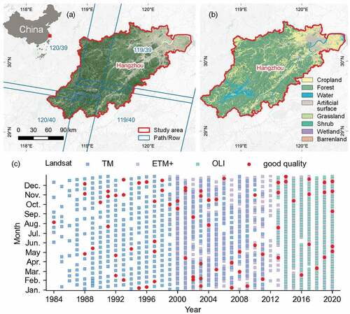
Hangzhou was selected as the study area for the following reasons. (1) The city is within a coastal region with frequent cloudy weather, with the result that cloud-free Landsat images are difficult to collect, especially from late spring to early autumn (Figure 1(c)). (2) The city crosses the side-lap regions of Landsat image swaths (Figure 1(a)), and it is rarely possible to match a set of cloud-free images with near acquisition dates. (3) More than four fifths of the city are covered by vegetation (Figure 1(b)), providing favorable conditions for exploring phenology-induced uncertainties.

2.2. Dataset

2.2.1. Image data

A total of 4348 available level-1 Landsat images acquired during 1984–2020 were collected for scenes 119/39, 119/40, 120/39, and 120/40. The number of available Landsat images for each scene was slightly different, with a minimum of 1054 for 120/40 and a maximum of 1121 for 119/39. The image distribution from different sensors is quite similar among scenes. For example, there were 518 images from Landsat-5 TM (1 June 1984 to 3 November 2011), 432 images from Landsat-7 ETM+ (6 August 1999 to 21 December 2020), and 171 images from Landsat-8 OLI (14 April 2013 to 29 December 2020) for scene 119/39 (Figure 1(c)). For each Landsat image, 8 bands were used, including six optical bands (Blue, Green, Red, NIR, SWIR1, and SWIR2), one thermal infrared (TIR) band, and a Quality Assessment (QA) band.

2.2.2. Impervious surface data

Impervious Surface Percentage (ISP) data for three periods (2000, 2005, 2010), with the spatial resolution of 500 m, were downloaded from the Geographical Simulation and Optimization Systems (GeoSOS, www.geosimulation.cn/ISA-China.htm). This data was generated from DMSP-OLS and MODIS images. Numerous studies have shown that ecological conditions are strongly correlated with the ISP and that an increase in the ISP degrades the ecological conditions (Yingchun et al. 2019; Xi Sheng and Han Qiu 2018; Huidong et al. 2018). The ISP data was correlated with the RSEI to provide a quantitative assessment of the model accuracy.

2.2.3. Training data

The training data was collected from the Globeland30 land cover maps (http://www.globallandcover.com/) for the three periods of 2000, 2010, and 2020. These maps have been recently accepted as a useful reference for land use studies because they provide 10 land cover categories (cultivated land, forest, grassland, shrubland, wetland, water, tundra, artificial surface, bare land, snow/ice) worldwide, and with the spatial resolution of 30 m (Jun, Fang Ban, and SongvNian 2014). We designed a general sampling rate of 0.2, meaning that ~20% of the total pixels of the study area were randomly selected as training samples. This percentage was obtained from the manual of the CCDC algorithm, and it has proven to provide the best classification performance based on the testing of different sample sizes of a training dataset (Zhou et al. 2020). To maximize classification performance, additional constraints were designed: there was no category with a sample rate <0.01 or >0.05, which ensured an approximately proportional representation of each category. If the pixels for a category accounted for >5% of the total pixels, only 5% of the pixels would be randomly selected; and if the pixels for a category accounted for <1%, all available pixels would be collected with no selection.

3. Methodology

3.1. CCDC algorithm

3.1.1. Data pre-processing

Instead of using the original DN values, we derived surface reflectance (for the optical bands) or brightness temperature (for the TIR band) for all Landsat images (Figure 2(a)). The acquisition of surface reflectance for Landsat-5 and −7 images used the 6S radioactive transfer model, which was processed by the Landsat Ecosystem Disturbance Adaptive Processing System (LEDAPS, https://pubs.er.usgs.gov/publication/ofr20131057). The surface reflectance for Landsat-8 images was obtained from the Landsat-8 Surface Reflectance (L8SR) system with an internal algorithm. The QA band for each image was retained during the processing.

Figure 2. General framework for mapping the time-series Remote Sensing–based Ecological Index (ts-RSEI).

Subsequently, we separated clear-sky observations from invalid or cloud-contaminated observations, which is important for accurately describing the phenology and other aspects of the land surface (Figure 2(a)). First, observations with invalid data values were removed. For the surface reflectance bands with the INT16 format, the valid data range was set to [0, 10,000]. The valid data range for brightness temperature bands was set to [2630, 3300] (i.e. −10–60°C), after considering the local climatic conditions. Second, cloud-contaminated observations were removed using two steps (Figure 2(a)). The QA band, generated by the Function of Mask (FMask) algorithm (Zhu et al., 2015a), was initially used to filter clouds, cloud shadows, snow, and the Scan Line Corrector (SLC) off gaps (for Landsat-7 images). Despite this filtering, there was a high possibility of observations with ephemeral noise (e.g. undetected clouds, cloud shadows, atmospheric haze, smoke) remaining within the images, and therefore we employed a multiTemporal Mask (TMask) algorithm to further remove these outliers (Zhu et al., 2015b). The TMask-identified observations that deviated significantly from the overall trend were only implemented at the initialization of the time-series models.

3.1.2. Model construction and change detection

(1) Piecewise linear harmonic model

Land surface change is typically divided into periodic intra-annual changes, gradual inter-annual changes, and abrupt changes (Wang et al. 2022; Zhu and Woodcock 2014). Therefore, a piecewise linear harmonic time-series model was used to fully describe the entire spectrum of land surface changes. For each pixel of the Landsat images, the piece number of the time-series model depended on the abrupt changes detected, and at least one piece was established for each band. For each piece, three candidate time-series models, comprising a linear and a harmonic segment, were used to describe surface reflectance:

(1) $\hat{\rho }(i,t{)}_1=c_{0,i}+c_{1,i}t+a_{1,i}cos(\mathrm{w}t)+b_{1,i}sin(\mathrm{w}t)$(1)

(2) $\hat{\rho }(i,t{)}_2=c_{0,i}+c_{1,i}t+\sum _{n=1}^2{a}_{n,i}cos(n\mathrm{w}t)+b_{n,i}sin(n\mathrm{w}t)$(2)

(3) $\hat{\rho }(i,t{)}_3=c_{0,i}+c_{1,i}t+\sum _{n=1}^3{a}_{n,i}cos(n\mathrm{w}t)+b_{n,i}sin(n\mathrm{w}t)$(3)

Here, i is the i^th Landsat band; t is the Julian date; w is a constant representing the annual frequency (2π/365.25); c_0,i and c_1,i are the estimated intercept and slope coefficients, respectively, representing gradual inter-annual change; a_n,_i and b_n,_i are the estimated n^th (n = 1, 2, 3)–order harmonic coefficients, representing periodic intra-annual changes; and $\hat{p}{\left(i,t\right)}_n$ denotes the predicted surface reflectance for the n^th candidate time-series model.

The difference among candidate time-series models lies mainly in the complexity of the harmonic segment. The more complex the harmonic segment, the better the performance in capturing intra-annual variations. For example, the second time-series model (Equation 2(2) $\hat{\rho }(i,t{)}_2=c_{0,i}+c_{1,i}t+\sum _{n=1}^2{a}_{n,i}cos(n\mathrm{w}t)+b_{n,i}sin(n\mathrm{w}t)$(2) ) is superior to the first (Equation 1(1) $\hat{\rho }(i,t{)}_1=c_{0,i}+c_{1,i}t+a_{1,i}cos(\mathrm{w}t)+b_{1,i}sin(\mathrm{w}t)$(1) ) in describing bimodal characteristics. Except for the first time-series model used for model initialization with the TMask algorithm, the selection of the time-series model depended on the number of clear-sky observations (Figure 2(a)). If the number was 24 or greater, the third time-series model (Equation 3(3) $\hat{\rho }(i,t{)}_3=c_{0,i}+c_{1,i}t+\sum _{n=1}^3{a}_{n,i}cos(n\mathrm{w}t)+b_{n,i}sin(n\mathrm{w}t)$(3) ) would be selected; if the number was >18 and <24, the second time-series model would be selected; and otherwise, the first time-series model would be accepted. We used Least Absolute Shrinkage and Selection Operator (LASSO) regression to estimate the coefficients for all time-series models (Figure 2(a)), because LASSO has been demonstrated to effectively reduce instances of over-fitting by minimizing the sum of the absolute values of the coefficients and forcing a subset of coefficients to zeros (Friedman, Hastie, and Tibshirani 2010).

(2) Change detection

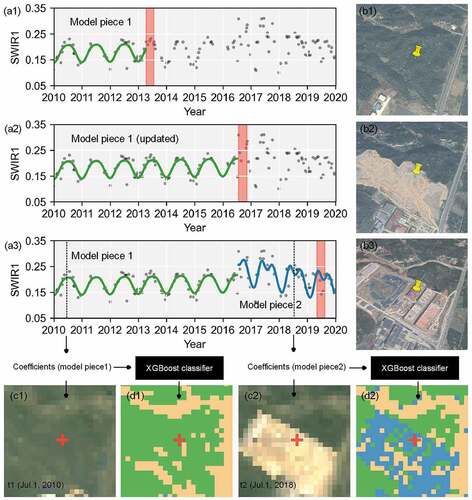
The break days for each piece were determined by comparing time-series model predictions with clear-sky observations (Figure 2(b)). We quantified the deviations between the predictions and observations using the combination of two measurements: the Root Mean Square Error (RMSE) and the Overall Variability (OVar). The RMSE was calculated using the 24 observations covered by the time-series model which were closest to the detected observations; alternatively, all the observations covered by the time-series model were used if there were fewer than 24. The OVar is computed as the median of the absolute value of the differences between each observation and the i^th successive observation, where i is the smallest value that most of the observation pairs are separated by more than 30 days. We used all Landsat bands, except for Blue and TIR, to detect land surface changes. The threshold for change detection (15.1) was obtained from an inverse distribution with the degrees of freedom equal to the band numbers. Given that ephemeral noise may remain after data filtering, 6 consecutive observations processed together were used rather than a single observation for accurate change detection (Figure 2(b), Figure 3 (a1)). Specifically, if the result was larger than the threshold for 6 consecutive times (Equation 4(4) $\sum _{i\in D}{\left(\frac{resi{d}_i}{max\left(RMS{E}_i,OVa{r}_i\right)}\right)}^2>15.1\left(\mathrm{f}\mathrm{o}\mathrm{r}6\mathrm{c}\mathrm{o}\mathrm{n}\mathrm{s}\mathrm{e}\mathrm{c}\mathrm{u}\mathrm{t}\mathrm{i}\mathrm{v}\mathrm{e}\mathrm{o}\mathrm{b}\mathrm{s}\mathrm{e}\mathrm{r}\mathrm{v}\mathrm{a}\mathrm{t}\mathrm{i}\mathrm{o}\mathrm{n}\mathrm{s}\right)$(4) ), a break day was determined as the date of the first observation (Figure 3 (a2, a3)); and if the result was larger than the threshold for only a few times, the relevant observations would be further detected if they were ephemeral noise that should be removed. When no change was detected, new clear-sky observations were added to the time-series, enabling the time-series model to self-update over time (Figure 3 (a1, a2)). The procedure is as follows:

Figure 3. Mechanism of Continuous Change Detection and the Classification (CCDC) algorithm. (a1–a3) Process of capturing Land Use and Cover Changes (LUCC) using a piecewise linear harmonic model, using the reflectance of the SWIR1 band as an example. The green and blue curves correspond to different model pieces before and after LUCC. (b1–b3) Google Earth history snapshots acquired from the periods labeled by the red rectangles in (a1–a3). The yellow pin corresponds to the location where the CCDC algorithm was applied. (c1–c2) Synthetic Landsat images for 1 July 2010 and 1 July 2018, generated by model coefficients. (d1–d2) Classification maps for Jul.1, 2010 and Jul.1, 2018, generated by XGBoost classifiers. The red cross corresponds to the pixel where the CCDC algorithm applies.

(4) $\sum _{i\in D}{\left(\frac{resi{d}_i}{max\left(RMS{E}_i,OVa{r}_i\right)}\right)}^2>15.1\left(\mathrm{f}\mathrm{o}\mathrm{r}6\mathrm{c}\mathrm{o}\mathrm{n}\mathrm{s}\mathrm{e}\mathrm{c}\mathrm{u}\mathrm{t}\mathrm{i}\mathrm{v}\mathrm{e}\mathrm{o}\mathrm{b}\mathrm{s}\mathrm{e}\mathrm{r}\mathrm{v}\mathrm{a}\mathrm{t}\mathrm{i}\mathrm{o}\mathrm{n}\mathrm{s}\right)$(4)

Here, D is the Landsat bands used for change detection; i is the i^th Landsat band; resid_i is the residual relative to the LASSO model; and RMSE_i and OVar_i are the RMSE and overall variability, respectively.

3.1.3. Image synthesis and classification

(1) Image synthesis

For each pixel, integrating the time variable (t: Julian date) into the corresponding pieces of the time-series models enabled us to obtain the predicted surface reflectance for each band (Figures 2, c, 3c1, c2). For most of the pixels and for most of the time this process works perfectly. However, between adjacent pieces of time-series model corresponding to the time before and after a change in the surface, there is often a period when the observations fluctuate too greatly to enable the initialization of another piece of the time-series model. This means that some pixels likely possess certain periods where no piece is available. In such cases we used the break day closest to the given date to determine an adequate time-series piece. If the given date was earlier than the break day, we projected the former piece of the time-series model backward to the given date to predict the surface reflectance and brightness temperature; otherwise, the latter piece was projected forward. In this way, the image at any date after 1984 could be synthesized. However, in our study, the images during 1986–2019 were synthesized because a certain length of time was needed to collect sufficient cloud-free observations for the initialization and termination of the time-series model.

(2) Image classification

eXtreme Gradient Boosting (XGBoost) was used for land cover classification (Figure 2(c)). XGBoost is a scalable implementation of gradient tree boosting, which delivers high performance and accuracy compared to other algorithms (Georganos et al. 2018). In our study, the fast histogram optimized approximate greedy algorithm was applied for tree generation and was assigned the values of 8 for the maximum tree depth and 500 for the number of trees. We used time-series model coefficients and RMSEs as input features (Figure 3 (d1, d2)). Specifically, for each band, 8 features were extracted, including one feature to represent the overall reflectance at a given date by combining the constant (c_0,i) and slope (c_1,i) coefficients, three pairs of coefficients (a_n,_i, b_n,_i, n = 1,2,3) to fully describe intra-annual changes, and an RMSE to measure the time-series model performance. Therefore, there was a total of 56 features from 6 optical bands and a TIR band as input features for XGBoost. The training data from the three phases were merged and inputted to XGBoost, and the resulting classifier was applied to predict classification maps at any given date.

3.2. RSEI construction

3.2.1. Index calculation

3.2.1.1. Greenness

Vegetation plays a critical role in natural systems as it participates in numerous biogeochemical cycles and contributes to the global energy balance (Yan et al. 2020). Greenness reflects many aspects of vegetation, including the number and type of plants and the growth and coverage conditions. The NDVI, which is based on the reflection features in the near-infrared and red wavelengths by plant leaf surfaces, has been successfully applied to monitor and assess greenness across different scales. Thus, the NDVI was employed to represent greenness (Figure 2(d)), and it can be calculated as in Equation 5(5) $NDVI=\frac{{\rho }_{NIR}-{\rho }_{Red}}{{\rho }_{NIR}+{\rho }_{Red}}$(5) .

(5) $NDVI=\frac{{\rho }_{NIR}-{\rho }_{Red}}{{\rho }_{NIR}+{\rho }_{Red}}$(5)

Here, ρ_NIR and ρ_Red denote the NIR and Red bands from synthetic Landsat images, respectively.

3.2.1.2. Dryness

Surface dryness has two main sources: artificial impervious surfaces and natural bare soil. As a result of ongoing urbanization, artificial impervious surfaces accelerate land dryness by altering biogeochemical processes and circulation patterns (Han Qiu 2008). Naturally bare soils, in the form of patches of bare land, areas of sparse vegetation, or transitions during land use change, also cause dry conditions (Deng et al. 2015; Jamali, Ali Montazeri Naeeni, and Zarei 2020). Accordingly, dryness was measured by the Normalized Difference Building and Soil Index (NDBSI, Figure 2(d), Equation 6(6) $NDBSI=\frac{IBI+SI}{2}$(6) ), a combination of the Index-based Built-up Index (IBI, Equation 7)(7) $IBI=\frac{\frac{2{\rho }_{SWIR1}}{{\rho }_{SWIR1}+{\rho }_{NIR}}-(\frac{{\rho }_{NIR}}{{\rho }_{NIR}+{\rho }_{Red}}+\frac{{\rho }_{Green}}{{\rho }_{Green}+{\rho }_{SWIR1}})}{\frac{2{\rho }_{SWIR1}}{{\rho }_{SWIR1}+{\rho }_{NIR}}+(\frac{{\rho }_{NIR}}{{\rho }_{NIR}+{\rho }_{Red}}+\frac{{\rho }_{Green}}{{\rho }_{Green}+{\rho }_{SWIR1}})}$(7) and the Soil Index (SI, Equation 8(8) $SI=\frac{({\rho }_{SWIR1}+{\rho }_{Red})-({\rho }_{NIR}+{\rho }_{Blue})}{({\rho }_{SWIR1}+{\rho }_{Red})+({\rho }_{NIR}+{\rho }_{Blue})}$(8) ), taking both sources into account. They are calculated as follows:

(6) $NDBSI=\frac{IBI+SI}{2}$(6)

(7) $IBI=\frac{\frac{2{\rho }_{SWIR1}}{{\rho }_{SWIR1}+{\rho }_{NIR}}-(\frac{{\rho }_{NIR}}{{\rho }_{NIR}+{\rho }_{Red}}+\frac{{\rho }_{Green}}{{\rho }_{Green}+{\rho }_{SWIR1}})}{\frac{2{\rho }_{SWIR1}}{{\rho }_{SWIR1}+{\rho }_{NIR}}+(\frac{{\rho }_{NIR}}{{\rho }_{NIR}+{\rho }_{Red}}+\frac{{\rho }_{Green}}{{\rho }_{Green}+{\rho }_{SWIR1}})}$(7)

(8) $SI=\frac{({\rho }_{SWIR1}+{\rho }_{Red})-({\rho }_{NIR}+{\rho }_{Blue})}{({\rho }_{SWIR1}+{\rho }_{Red})+({\rho }_{NIR}+{\rho }_{Blue})}$(8)

Here, ρ_Blue,ρ_Green,ρ_Red,ρ_NIR, and ρ_SWIR1 respectively denote the Blue, Green, Red, NIR, and SWIR1 bands from synthetic Landsat images.

3.2.1.3. Humidity

The first three components after the Tasseled Cap Transform (TCT) have significant environmental implications, especially the third factor – Wetness – and it has been proven to be an effective index to represent land surface moisture (Crist 1985). Therefore, the Wetness component was considered to represent humidity (Figure 2(d)).

It should be noted that the TCT was implemented using linear combinations of each band with the empirical selection of coefficients, which means that the coefficients tend to vary among sensors. Previous studies used true Landsat images with accurate sensor information (e.g. TM, ETM+, OLI) that established transformation equations that can be used directly (Baig et al. 2014; Crist 1985; Huang et al. 2002). However, for synthetic Landsat images it is difficult to determine how to apply the established transformation equations because the information used for generating each pixel is likely to be different. This relates strongly to the length and location of the piece of the time-series model used by a pixel; this information may come from a single sensor if the piece is short and acquired at an early stage, otherwise, the information can even be an integration of the three sensors (e.g. the pixel generated by the first piece of the time-series model was fitted by the observations for 2010–2016 when the information from TM, ETM+, and OLI was involved, Figure 3 (a2)). For simplicity, the initial Wetness from each sensor was calculated individually based on previously-established transformation equations and then averaged to produce the final Wetness. Given that the TCT is a linear function, the average of the initial Wetness is equivalent to the average of the corresponding coefficients. Thus, the Wetness from synthetic Landsat images was defined according to Equation 9(9) $Wetness=0.1484{\rho }_{Blue}+0.3068{\rho }_{Green}+0.2437{\rho }_{Red}+0.1886{\rho }_{NIR}-0.7184{\rho }_{SWIR1}-0.5352{\rho }_{SWIR2}$(9) .

(9) $Wetness=0.1484{\rho }_{Blue}+0.3068{\rho }_{Green}+0.2437{\rho }_{Red}+0.1886{\rho }_{NIR}-0.7184{\rho }_{SWIR1}-0.5352{\rho }_{SWIR2}$(9)

Here, ρ_Blue,ρ_Green,ρ_Red,ρ_NIR,ρ_SWIR1, and ρ_SWIR2 denote Blue, Green, Red, NIR, SWIR1, and SWIR2 bands from synthetic Landsat images, respectively.

3.2.1.4. Heat

LST is a useful index for the measurement of heat because it is closely related to the growth and distribution of vegetation, crop yield, and evaporation from surface water. In this study, LST was obtained using an emissivity modulation method, which has been proven to be accurate for temperature retrieval (Nichol 2005). For the brightness temperature band (T_b) of synthetic Landsat images, LST was calculated using Equations 10(10) $LST=\frac{T_b}{1+\frac{\lambda T_b}{\alpha }ln\epsilon }$(10) and 11(11) $\alpha =\frac{\mathrm{h}\mathrm{c}}{\mathrm{K}}$(11) .

(10) $LST=\frac{T_b}{1+\frac{\lambda T_b}{\alpha }ln\epsilon }$(10)

(11) $\alpha =\frac{\mathrm{h}\mathrm{c}}{\mathrm{K}}$(11)

Here, h is the Planck constant (6.26 × 10⁻³⁴ J-sec), c is the velocity of light (2.998 × 10⁸ m/sec), K is the Boltzmann constant (1.38 × 10⁻²³ J/K), and λ denotes the central wavelength (μm) for the corresponding TIR band (i.e. 11.48 × 10⁻⁶ for band 6 of Landsat TM/ETM+ images, and 10.90 × 10⁻⁶ for band 10 of Landsat OLI images). Like the processes for averaging the coefficients during TCT transformation, λ was set as 11.19 × 10⁻⁶ for synthetic Landsat images; and ε denotes the surface emissivity, referenced by (Nichol 2005), which varies according to the land cover. Specifically, we set ε as 0.97, 0.91, 0.92, 0.95, 0.99, and 0.97 for forest, grassland, artificial surface, bare land, water, and other vegetation types, respectively. This process was easily conducted with the assistance of classification maps, which were simultaneously generated with synthetic Landsat images (Figure 2(d)).

3.2.2. Index post-processing

Except for the common post-processing method for individual indices such as the water mask (Han Qiu 2006), we used two other methods to preserve the reality and consistency for the long-term description of ecological quality (Figure 2(d)):

3.2.2.1. Outlier modification

Previously, individual indices were directly normalized with relatively little consideration given to outliers; however, a very few extremely large or small outliers were observed in the original indices (Figure S1a1–c1 of supplementary materials), especially for a large study area or a long-term study. If these outliers are not rectified, normalization using the maximum and minimum values from the outliers would significantly bias the data distribution (Figure S1a2–c2 of supplementary materials) and induce uncertainty. Therefore, we used an outlier modification method using a percentile, which was set as 0.5 so that values exceeding the range between the 0.5% and 99.5% percentiles were regarded as outliers and modified. Specifically, the values corresponding to the 0.5% and 99.5% percentiles were validated as the minimum and maximum, respectively. Any value less than (greater than) the validated minimum (maximum) was assigned to the validated minimum (maximum). A total of 1% of the values were modified during this process.

3.2.2.2. All-time normalization

Previously, the normalization of the original indices was conducted for each study period separately, but this may be inappropriate. An index likely represents a long-term trend, with the values from a later image overall rising or falling relative to a previous image by a certain magnitude. This phenomenon results from climatic variability, vegetation growth, or land degradation (Zhu and Woodcock 2014). However, the true magnitude may be offset when such an individual normalization method is implemented. For example, the original distribution of NDVI values is distinct between 1987 and 2017, indicating a potential greening process over 30 years (Figure S1a1–c1 of supplementary materials). After individual normalization, however, the NDVI ranges of the two years were identical and the NDVI distributions was similar (Figure S1a2–c2 of supplementary materials). Therefore, we used an all-time normalization method that uses two fixed boundaries (lower and upper) for normalizing indices from all the periods. For a specific index, the minimum (maximum) for the validated minima (maxima) from all periods was defined as the lower (upper) boundary. Therefore, although the data range for a specific period may not completely reach [0, 1] after all-time normalization, a reasonable distribution of an index can be obtained, from a long-term perspective (Figure S1a3–c3 of supplementary materials).

3.2.3. PCA transformation

PCA is a multi-dimensional data compression technique that can eliminate the effect of co-linearity among the original variables. The weight for each variable is automatically allocated according to the varying contributions, preventing errors in manual weight assignment (Chen et al. 2014). Therefore, PCA was used to integrate the post-processing indices of greenness, dryness, humility, and heat (Figure 2(e)). Note that in previous studies PCA transformation was separately implemented for each study period, resulting in several PCA models with different weights. Since the temporal resolution of synthetic Landsat images can be set to a very fine scale, the weights for each period should be uniform to avoid any detected ecological changes being induced by weight differences. Therefore, we generated a unique PCA model using the synthetic Landsat images from all periods.

The first principal component subtracted from 1 was taken as the initial ts-RSEI (ts-RSEI₀, Equation 12(12) $ts-RSE{I}_0=1-\mathrm{P}\mathrm{C}\mathrm{A}1(NDVI,NDBSI,Wetness,LST)$(12) ), in accordance with the general recognition that higher values should indicate better ecological conditions. To facilitate temporal comparisons, we also conducted outlier modification and all-time normalization processes to obtain the final ts-RSEI (Figure 2(e), Equation 13)(13) $ts-RSEI=\frac{ts-RSE{I}_0-ts-RSE{I}_{lb}}{ts-RSE{I}_{ub}-ts-RSE{I}_{lb}}$(13) . All the annual images were merged to construct a single PCA transformation model for which the percentage covariance eigenvalue of the ts-RSEI reached 71.8%; the loadings for the four indicators (greenness, dryness, humility, and heat) on the ts-RSEI were 0.713, −0.427, 0.540, and −0.128, respectively.

(12) $ts-RSE{I}_0=1-\mathrm{P}\mathrm{C}\mathrm{A}1(NDVI,NDBSI,Wetness,LST)$(12)

(13) $ts-RSEI=\frac{ts-RSE{I}_0-ts-RSE{I}_{lb}}{ts-RSE{I}_{ub}-ts-RSE{I}_{lb}}$(13)

Here, PCA1 is the first principal component from the PCA, and ts-RSEI_lb and ts-RSEI_ub are the mean lower and upper boundaries of ts-RSEI₀.

4. Results

4.1. Sensitivity of the RSEI to the timespan of observations

To measure the influence of the timespan of observations, we calculated and compared RSEI differences based on pairwise cloud-free real Landsat images with acquisition dates <32 days (~1 month). Scene 119/39 was selected to conduct the process since it covers most of the study area; additionally, scene 119/39 has a variety of land use and cover types, such as forest, cropland, and artificial surfaces, with relatively even proportions of these land-use types (Figure 1(b)).

All available pairs of real Landsat images were collected during 1984–2020, including 2 pairs with the timespan of 8 days, 4 pairs with the timespan of 16 days, and 5 pairs with the timespan of 32 days. For the pairwise image with the timespan of 8 days, the difference between their derived RSEI values was small, with 0.065 as the Mean Absolute Difference (MAD) calculated for each pixel (Figure 4(a)). The RSEI difference for each pixel appeared to be random and evenly distributed, represented by a normal distribution with the mean of zero (Figure 5(a)). However, the RSEI difference increased significantly when the timespan of the pairwise images was increased. The MAD of the derived RSEI was 0.094 between pairwise image with the timespan of 16 days, and it reached 0.111 for the timespan of 32 days (Figure 4(a)). Additionally, the RSEI difference for each pixel became systematic as the timespan of the pairwise image increased – the RSEI difference was likely to be positive when the pairwise image was acquired after August, and vice versa. For example, although the RSEI difference between the image pair acquired for Sep. 17 and 3 October 2000 was still around zero, a larger number of pixels with a positive difference were observed, leading to a biased normal distribution (Figure 5(b)). The RSEI difference between the images acquired for Nov. 3 and 5 December 1988 was normally distributed, but the center had shifted to a positive value (~0.09, Figure 5(c)). This rapid increase in systematic differences indicated a relatively high sensitivity of the RSEI to the timespan of the observations.

Figure 4. Absolute difference distributions for the pairwise RSEI calculated using real and synthetic Landsat images. The absolute difference distributions for the overall area (a) and main land use and cover types (b) are calculated using the pairwise RSEI derived from real Landsat images with different timespans. The monthly absolute difference distributions for the overall area (c) and main land use and cover types (d) are calculated using the pairwise RSEI derived from real and synthetic Landsat images. The mean absolute differences (MAD) are labeled with dashed lines: blue for the overall area, green for forest, yellow for cropland, and red for artificial surfaces. Gray numbers denote the image numbers used for calculation.

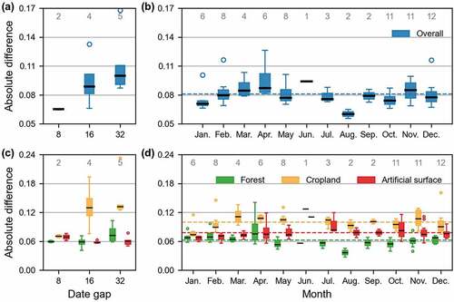
Figure 5. Differences in pairwise RSEI between real Landsat images with different timespans. The first and second columns are the RSEIs calculated for the real Landsat images for two adjacent periods. The timespan between the first and second columns increases by rows, 8 days for (a), 16 days for (b), and 32 days for (c). The third column shows the RSEI differences between the first and second columns, with the outstanding differences labeled with land use and cover type. The fourth column shows a histogram of the RSEI differences and the Mean Absolute Difference (MAD).

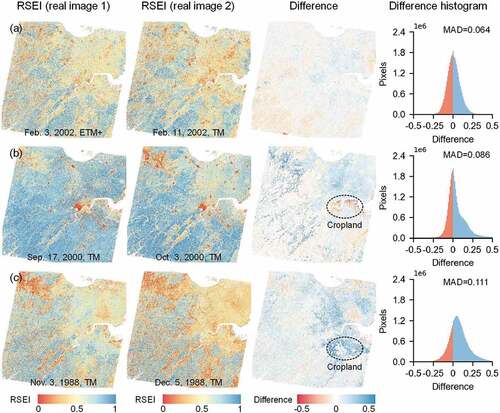
The RSEI sensitivity was observed to vary among land use and cover types (Figure 4(b)). For land use types that change frequently, like cropland, the RSEI sensitivity was high, especially for a timespan greater than 8 days (the MAD almost doubled as the timespan increased to 16 days). For forest, an RSEI sensitivity began to emerge when the timespan exceeded 16 days; but for artificial surfaces, there was no obvious trend in RSEI sensitivity with increasing timespan.

4.2. Accuracy assessment of the ts-RSEI

The uncertainty of ts-RSEI maps mainly come from two aspects: the RSEI model and CCDC technology.

4.2.1. Accuracy of the RSEI model

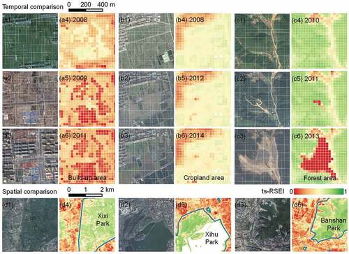
We evaluated the accuracy of the RSEI model using both qualitative and quantitative means. Three LUCC events occurring in built-up areas, cropland, and forested areas were introduced for qualitative assessment (Figure 6). In a typical built-up area, inner cropland was converted to urban land during 2008–2011 (Figure 6 (a1–a3)). This process was manifested by a decrease from 0.46 to 0.11 of the average value of a clustered area of more than 1 million m² in the ts-RSEI maps (Figure 6 (a4–a6)). The capability of identifying tiny LUCC changes in space and time for the ts-RSEI maps was also evaluated. For example, several houses were continuously constructed in the cropland areas during 2008–2014 (Figure 6 (b1–b3)). Such pixel-level changes were accurately detected by the ts-RSEI maps, with the value for 11 pixels decreasing from 0.48 to 0.37 (Figure 6 (b4–b6)). The ts-RSEI maps even captured the initial moment of quarry establishment in 2011 (Figure 6 (c2)), reflected by a large decrease in the average values of 6 pixels (Figure 6 (c5)). For the same land-use types, ts-RSEI maps can differentiate in detail the values that reflect the influences from different backgrounds. This was validated by three urban parks and their peripheral areas (Figure 6 (d1–d6)). The ts-RSEI values for artificial surfaces in the urban parks averaged 0.21, which was ~0.10 lower than those in the peripheral areas within a 1 km buffer. This makes sense because parks have favorable conditions in terms of wetness and temperature.

Figure 6. Temporal and spatial validation of ts-RSEI maps. Temporal validation was conducted for three typical sites – a built-up area (a), cropland (b), and forest (c) – before and after Land Use and Cover Change (LUCC). Sub-figures 1–3 show Google Earth snapshots before and after LUCC; and sub-figures 4–6 show ts-RSEI maps before and after the LUCC. Spatial validation was conducted on the three urban parks (and adjacent areas) of Xixi, Xihu, and Banshan. Sub-figures 1–3 and 4–6 show Google Earth snapshots and ts-RSEI maps, respectively.

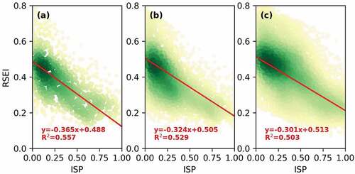
The correlations between the ts-RSEI and ISP for the whole area for the three periods (2000, 2005, and 2010) were used for quantitative assessment. After generating and re-sampling ts-RSEI maps with the same temporal and spatial resolutions, we used linear regression to determine the correlation between the ts-RSEI and ISP (Figure 7). The limited deviations of most of the points from the best-fit line indicated a good performance, with the coefficient of determination (R²) for the three periods exceeding 0.5. Several outliers are evident, probably due to the limited ability of the ts-RSEI maps to differentiate values for the same land use with varying backgrounds. The slopes of the best-fit lines for the three periods are all negative (~-0.3), in agreement with common sense. The changes in both the slopes and intercepts (~0.5) of the best-fit lines are only slightly different for the three periods, indicating the stability of the correlation and the validity of the RSEI model.

Figure 7. Correlations between the ts-RSEI and the Impervious Surface Percentage (ISP) for the years 2000 (a), 2005 (b), and 2010 (c).

(2) Reliability of the CCDC algorithm

We compared the difference between the ts-RSEI derived from synthetic Landsat images and the RSEI derived from real Landsat images with the same acquisition dates, with the objective of quantitatively evaluating the reliability of the CCDC algorithm. A total of 74 pairs of comparisons were involved this process, in accordance with the number of cloud-free real Landsat images from scene 119/39 (Figure 1(c)).

The ts-RSEI derived from synthetic images was very similar to the RSEI from the real images. A normal distribution with a mean of zero can be observed from the difference between the ts-RSEI and RSEI for each period and season, indicating that the difference was probably random rather than systematic (Figure 8). Monthly analyses further revealed an obvious intra-annual trend for the absolute differences between the ts-RSEI and RSEI (Figure 4(c)). Specifically, the absolute differences were small during summer (e.g. average of 0.060 for August) and winter (e.g. average of 0.075 for January). However, for the other two seasons, the absolute differences became larger, especially for mid-spring (April) when the vegetation grows rapidly, for which the average reached 0.095.

Figure 8. Differences between the RSEI and ts-RSEI from real and synthetic Landsat images with the same date. The first and second columns are the RSEIs and ts-RSEIs calculated for real and synthetic Landsat images. Difference between the RSEI and ts-RSEI by season and decade, including spring in the 1980s (a), summer in the 2000s (b), autumn in the 2010s (c), and winter in the 1990s (d). The third column shows the differences between the first and second columns, with the outstanding differences labeled with the land use and cover type. The fourth column shows a histogram of the differences and the Mean Absolute Difference (MAD).

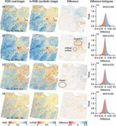
The absolute difference between the ts-RSEI and RSEI among the land use and cover types tended to vary (Figure 4(d)). Among the three main types, the absolute difference for forest was the lowest and reached a minimum (0.036) during summer. The absolute difference for cropland was the highest and usually reached a maximum (0.113) during spring or autumn. For artificial surfaces, the absolute difference was minor, and the intra-annual fluctuation was not significant, except for a slight increase during summer. The MAD between the ts-RSEI and RSEI for forest and artificial surfaces was 0.062 and 0.078, respectively, which was almost the same as that of the RSEI between real images with the timespan of 8 days. The MAD between ts-RSEI and RSEI for cropland was 0.099, which was intermediate to that of the RSEI between real images with the timespan of 8–16 days (Figure 4(b, d)).

The MAD between the ts-RSEI and RSEI was 0.082, slightly higher than the MAD of the RSEI between real images with the timespan of 8 days but obviously lower than the images with the timespan of 16 days (Figure 4(a, c)). In fact, the value 0.075 of the MAD between the ts-RSEI and RSEI in summer may be more meaningful, since in most cases this season is used for ecological quality assessment. Since the average RSEI of our study area was ~0.719 during summer, an MAD of 0.075 corresponds to a 10.5% error, demonstrating the relatively high accuracy of the ts-RSEI derived from synthetic Landsat images.

4.3. Spatio-temporal changes in ecological quality

Our methods enabled us to generate ts-RSEIs for any time interval, and annual ts-RSEI maps were used as an example. The synthetic Landsat images for Jul. 1 of each year during 1986–2019 were generated. The annual ts-RSEI maps revealed continuous changes in ecological quality during 1986–2019, and even subtle changes could be tracked (Figure 9). In general, the overall ecological quality of Hangzhou was maintained over the past 35 years, evidenced by the change of the mean ts-RSEI from 0.679 to 0.705 (Figure 10(a)). Compared with only a slight change in the mean value, the standard deviation of the ts-RSEI increased substantially, indicating the likely existence of regional divergences in changes in ecological quality.

Figure 9. Spatial divergence of ecological quality in Hangzhou during 1986–2019 evaluated by annual ts-RSEI. For each annual ts-RSEI, the date of Jul. 1 of the corresponding year was used.

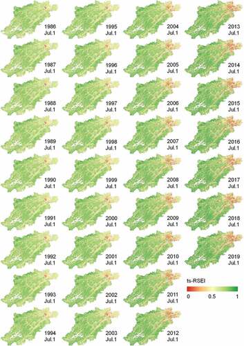
Figure 10. Annual changes in ecological quality in Hangzhou during 1986–2019. The mean values (points) and standard deviations (error bars) of the ts-RSEI are used to depict the ecological quality. Key turning points in ecological quality are labeled with the mean ts-RSEI value. Changes in ecological quality are evaluated for the overall area (a) and the main land use and cover types, including forest (b), cropland (c), and artificial surfaces (d). The area percentages for the main land use and cover types are shown as gray bars.

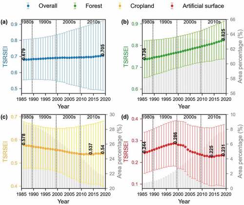
We then analyzed the changes in ecological quality for different land use and cover types. Forest is widespread southwest of Hangzhou, with the minimum coverage of 62.0%. The ecological quality for forest increased continuously, represented by an increase in the mean ts-RSEI from 0.736 to 0.825, which was the most prominent change among the three land-use and cover types (Figure 10(b)). The standard deviation of the ts-RSEI was almost unchanged throughout the past 35 years, implying an overall improvement in ecological quality. Further analysis revealed that this increase was mainly the result of the progressive greening of the forest (Figure 11(a, b)). In recent years, the global greening of vegetation due to climate change and CO₂ fertilization effects has been widely reported (Chen et al. 2019; Zhu et al. 2016), and the southeastern coast of China, where Hangzhou is located (Figure 11(e)), provides one of the most striking manifestations of this phenomenon.

Figure 11. Relative changes of the RSEI in relation to four relevant indices (greenness, dryness, humidity, and heat) during 1986–2019. (a) Relative changes of the four indices among the main land use and cover types, measured by differences in normalized indices. Note that the increases in dryness and heat represent a negative effect for ecological quality. Three typical regions with the four intervals of 1986, 1997, 2008, and 2019 are used to represent long-term changes in normalized greenness for forest (b), normalized humidity for cropland (c), and normalized heat for artificial surfaces (d). Photos taken in 2019 of Hangzhou to illustrate (e) the global greening phenomenon for the forest ecosystem, (f) the cropland degradation phenomenon due to decreasing humidity, and (g) the urban heat island effect caused by high-density built-up areas.

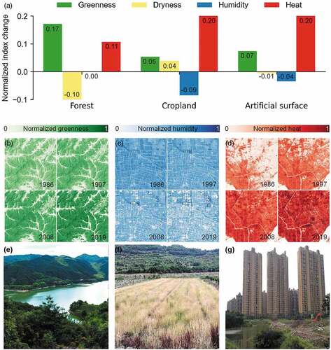
The cropland in northeastern Hangzhou experienced a general degradation in ecological quality as its area was substantially reduced (Figure 10(c)). Specifically, the ecological quality for cropland gradually decreased before 2014, after which there was a slight increase (shown by the decrease in mean ts-RSEI from 0.578 to 0.537), followed by an increase to 0.540. The ecological degradation of cropland is demonstrated by almost all the indices involved in ts-RSEI construction (Figure 11(a)). The decrease in humidity was an important reason for this degradation (Figure 11(b)), except for the heat island effect. Based on our field survey, the poor management of cropland (Figure 11(f)) was responsible for the decrease in humidity and the degradation of the ecological environment. There was a sharp increase in the extent of artificial surfaces, while the ecological quality generally decreased with fluctuations (Figure 11(d)). Before 1999, the mean ts-RSEI for artificial surfaces increased from 0.244 to 0.286, after which it rapidly decreased to 0.225. Despite a minor rebound after 2014, the ts-RSEI remained lower than the initial level. Given the relatively low vegetation coverage, heat may be more important than greenness in the case of artificial surfaces (Figure 11(a)). This effect was especially discernable after 2000 when high-density buildup areas became prevalent, with limited consideration given to greening facilities (Figure 11(c, g)).

It is noteworthy that the difference between nature-dominated (e.g. forest) and human-dominated environments (e.g. cropland and artificial surfaces) has increased, as evidenced by the trend of spatial polarization in regional ecological quality (Figure 9). For example, the difference in the mean ts-RSEI between natural and human-dominated environments has more than doubled during the past 35 years (0.168 in 1986 and increasing to 0.351 in 2019). This polarization implies that future conversions from a natural to a human-dominated environment should be considered carefully, because of the higher ecological costs that would be incurred.

Our methods also enabled us to conduct an assessment at a finer temporal resolution (e.g. semimonthly), to explore intra-annual changes in ecological quality. The synthetic Landsat images on the 10^th and 20^th day of each month in 2019 were used for semimonthly ts-RSEI maps, the spatio-temporal changes of which are shown in Figure S2 and S3 of the supplementary materials.

5. Discussion

5.1. Comparison of different methods for reconstructing RSEI

Our results demonstrate pronounced intra-annual RSEI changes in areas of high vegetation coverage; for reference, a timespan of 1 month will result in an MAD of 0.111 in Hangzhou, equivalent to a 19.2% relative error in the RSEI. This error is too large to ignore, and it may be even larger for the extensive cropland areas (Figure 4(b)).

The high sensitivity to the timespan of the observations is a major problem for image collection, with side-lap regions of image swaths, especially, leading to a small study area and few study periods in most previous studies. Given that Hangzhou spans 4 Landsat scenes, if cloud-free images were collected for RSEI construction, only 16 images from 4 periods (1997, 2000, 2010, 2017) would be available (Figure 12(a)). In terms of a comparison with the ts-RSEI, two points can be made. (i) The general trend of ecological quality evaluated by the foregoing cloud-free-image method was lower. This is probably because the selected images are from late spring (May). Although mid-summer (July or August) is the best period for ecological assessment, it is poorly accessible in terms of image collection due to the frequent cloudy weather. (ii) Only a minor amount of information was provided by the cloud-free-image method and there was a slight distortion. The method only revealed changes in ecological quality over 20 years within 4 discrete time slices, instead of providing information for tracking annual changes in ecological dynamics throughout the 35-year period. The rapid increase in ecological quality after 2000 is more likely caused by differences in image acquisition dates (closer to summer after 2000), rather than being a true reflection of reality. Additionally, the band reflectance from side-lap regions of a mosaic image usually showed a slight overall bias, even if the acquisition dates of the images were close (9 days, as shown in Figure 12(c)), which also introduces some degree of uncertainty in RSEI construction.

Figure 12. Comparison of methods for RSEI construction. (a) Performances of the three methods for RSEI construction based on continuous change detection (our approach), cloud-free images, and median value composition. (b1–b2) NDVI image composed of median values and its corresponding Day Of Year (DOY). (c) Mosaic image from two scenes of real Landsat images with near acquisition dates.

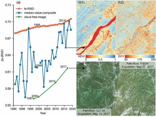
To overcome the problem of the poor accessibility of cloud-free images, several studies have begun to evaluate ecological quality annually or biennially, using image composition methods. A representative method is the median value composition, which uses all available images to calculate indices, after excluding observations contaminated by clouds and shadow; the median value for each pixel is extracted and used to compile an integrated image as a foundation for RSEI construction (Wang, Hao Zhao, and Jian Sheng 2020). Although the related indices generated by the foregoing method appear to be spatially continuous (Figure 12 (b1)), the annual RSEI between adjacent years fluctuated tremendously (Figure 12 (a)). This was caused mainly by the large differences among the dates corresponding to the extracted median values (Figure 12 (b2)), which was a more serious problem before 1999 because few annual Landsat images are available. Given that the individual RSEI for a specific year may involve a certain degree of error, it is arguably unsatisfactory to use the median-value-composite method to assess the general trend of ecological quality. Similarly, MODIS products, produced by maximum value composition, were usually used to monitor large-scale ecological quality (Han Qiu et al. 2019; Yuan et al. 2021). Despite their high temporal resolution, the collection of sufficient valid observations is not always easy within a short timespan (e.g. 16 days), especially in coastal areas during summer. As a result, the data for ecological assessment using MODIS products are still likely to omit some years (Han Qiu et al. 2019).

5.2. Implications and limitations of the ts-RSEI

The most significant contribution of this study is to propose the use of ts-RSEI time-series to assess the ecological quality using the RSEI. Essentially, the ts-RSEI was constructed by adjusting the RSEI to the CCDC technology, which provides a comparable degree of ecological quality assessment. This comparability comprises two aspects: first, the ecological assessment can be conducted at a fixed time (e.g. Jul. 1st of each year, the 10th day of each month), avoiding the errors from discrepancies in timespan; and second, the index post-processing enables the long-term trend (e.g. of vegetation growth, land degradation) to be reflected by the ecological assessment.

The reason we selected the RSEI as the indicator for ecological quality assessment is because it has been used in numerous regions worldwide. For China, the RSEI was applied in Fuzhou (Xi Sheng and Han Qiu 2018), Xiamen (Liu et al. 2021), Wuhan (Zhu et al. 2021) cities, and the Xiong’an new region (Han Qiu et al. 2018) for evaluating ecological quality. For the USA, the ecological quality for Minneapolis, Dallas, Phoenix, Seattle, and Chicago was compared using the RSEI (Firozjaei et al. 2021a). For Europe, urban surface ecological poorness zones in Madrid (Spain), Rome (Italy), Lyon (France), Hamburg (Germany), Ciechanow (Poland), and Budapest (Hungary) were identified using the RSEI (Firozjaei et al. 2021c). Given the potential for the inter-regional application of the RSEI, the international research community may be interested in adopting the ts-RSEI for tracking long-term changes in ecological quality using time-series analysis. Additionally, the CCDC algorithm is highly flexible in that it not only matches the Landsat images but it is also readily applicable to other images, such as Terra/Aqua MODIS (Tang et al. 2019) and Sentinel-2 MSI (Giannetti et al. 2021). In the near-future, the combination of the ts-RSEI from different images is expected to cover the ecological quality monitoring at multiple geographic scales: continental or national scales using MODIS derived ts-RSEI, regional scales using Landsat derived ts-RSEI, and local scales using Sentinel derived ts-RSEI.

Since the ts-RSEI was constructed according to the core concept of the RSEI (i.e. PCA transformation using the same remote sensing indices), the rationale for the use of ts-RSEI was determined to a large extent by the RSEI. Our results demonstrate that the uniform greening of the forested area was the main reason for the maintenance of the overall ecological quality in Hangzhou (Figure 10). It should be noted that the greenness was only measured by the NDVI in the RSEI (the PCA loading of greenness was 0.713). and whether the greenness can reliably reflect the ecological quality of the forest needs to be rigorously validated. This inevitably raises the issue of the rationale for the selected indices and weights. For example, Yang et al. (2020) proposed a Comprehensive Ecological Evaluation Index (CEEI), which substituted the NDVI for the Vegetation Cover (VC) and Vegetative Health Index (VHI), for evaluating the ecological quality of the Guangdong–Hong Kong–Macau Greater Bay Area of China. The CEEI may be superior to the RSEI given that more indices were used to evaluate the greenness (Jian Hui et al. 2021; Firozjaei et al. 2021b). Additionally, using the same indices as the RSEI, Firozjaei et al. (2021a) developed a Land Surface Ecological Status Composition Index (LSESCI), with the weights calculated using Ridd’s V-I-S triangle model, and confirmed the high efficacy of the LSESCI in discriminating ecological quality between bare soil and urban areas. Nevertheless, given the indices used in the above studies were derived from remote sensing images, our proposed method can be easily transferred to these indices since the CCDC technology enables the synthesis of images at any time.

Another issue is the indicative significance of the ts-RSEI. This indicator, which is composed of multiple single indices, can comprehensively measure the general trend of overall ecological quality, while the indicator itself may be more ambiguous compared to other indicators such as area or temperature. Nevertheless, the ts-RSEI-based ecological assessment for an area can contribute substantially to exploring continuous changes in ecological quality, such as changes in the ecological balance resulting from different land use and cover conversions, and ecological improvement/deterioration derived from long-term natural changes. Only by this means can a rational plan be formulated for balancing urban development with ecological conservation, which would be of great value to local authorities and policy makers.

6. Conclusions

The high sensitivity caused by the different acquisitions time of images has become a barrier to the widespread application of the promising Remote Sensing-based Ecological Index (RSEI). By modifying the RSEI to the Continuous Change Detection and Classification (CCDC) algorithm, we have mapped time-series RSEI (ts-RSEI) using synthetic Landsat images, which enabled us to monitor the dynamics of ecological quality at any time. Our results confirmed that the ts-RSEI from synthetic images was comparable to the RSEI from real images, with the relative error of only 10.5%, which is significantly lower than the RSEI from the two real images with the timespan of half-a-month. Compared with previous RSEI-reconstruction methods (e.g. cloud-free-image, median-value-composite), the ts-RSEI has outstanding advantages in terms of temporal consistency and accuracy of assessment. However, the subjectivity involved in selecting indices and weights and its ambiguous significance may be disadvantages for the use of ts-RSEI.

The ts-RSEI should be useful for policy makers and authorities in providing an accurate evaluation of ecological quality whenever needed, in order to facilitate ecological conservation. For example, the phenomenon of spatial polarization of ecological quality, especially for deteriorating human-dominated environments (e.g. farmland, artificial surfaces), should be of concern to the local government of Hangzhou. The method of using synthetic images to construct ts-RSEI has proven to be flexible, and it can be applied to other images (e.g. Terra/Auqa MODIS, Sentinel-2 MSI), and to other remote sensing–based ecological indicators (e.g. CEEI, LSESCI). Therefore, we expect the ts-RSEI to be extensively applied in the future.

Disclosure statement

No potential conflict of interest was reported by the author(s).

Data availability statement

All the Landsat images are freely downloaded in the LEDAPS at https://espa.cr.usgs.gov/, the Globeland30 land cover maps are freely downloaded at http://www.globallandcover.com/, and the CCDC codes used in this study are available in GitHub at https://github.com/GERSL/CCDC.

Supplementary material

Supplemental data for this article can be accessed online at https://doi.org/10.1080/15481603.2022.2138010.

Additional information

Funding

This work was suuported by the National Natural Science Foundation of China [41901121], the National Natural Science Foundation of China-Zhejiang Joint Fund for the Integration of Industrialization and Informatization [U1609203], the National Natural Science Foundation of China [41971378, 42206236], and the Natural Science Foundation of Zhejiang Province [LQ15D020001].

References

- Baig, M. H. A., L. Fu Zhang, T. Shuai, and Q. Xi Tong. 2014. “Derivation of a Tasselled Cap Transformation Based on Landsat 8 At-Satellite Reflectance.” Remote Sensing Letters 5 (5): 423–431. doi:10.1080/2150704X.2014.915434.
- Bowen, R. E., and C. Riley. 2003. “Socio-Economic Indicators and Integrated Coastal Management.” Ocean & Coastal Management 46 (3): 299–312. doi:10.1016/S0964-5691(03)00008-5.
- Buyantuyev, A., J. Wu, and C. Gries. 2007. “Estimating Vegetation Cover in an Urban Environment Based on Landsat ETM+ Imagery: A Case Study in Phoenix, USA.” International Journal of Remote Sensing 28 (1): 269–291. doi:10.1080/01431160600658149.
- Chen, M. X., W. Dong Liu, and L. Da Dao. 2016. “Challenges and the Way Forward in China’s New-Type Urbanization.” Land Use Policy 55: 334–339. doi:10.1016/j.landusepol.2015.07.025.
- Chen, Y. S., Z. Han Lin, X. Zhao, G. Wang, and G. Yan Feng. 2014. “Deep Learning-Based Classification of Hyperspectral Data.” IEEE Journal of Selected Topics in Applied Earth Observations and Remote Sensing 7 (6): 2094–2107. doi:10.1109/JSTARS.2014.2329330.
- Chen, C., T. Park, X. Hui Wang, S. Long Piao, X. Bao Dong, R. K. Chaturvedi, R. Fuchs, et al. 2019. “China and India Lead in Greening of the World through Land-Use Management.” Nature Sustainability 2 (2): 122–129. doi:10.1038/s41893-019-0220-7.
- Chen, J., M. Shen, X. Zhu, and Y. Tang. 2009. “Indicator of Flower Status Derived from in Situ Hyperspectral Measurement in an Alpine Meadow on the Tibetan Plateau.” Ecological Indicators 9 (4): 818–823. doi:10.1016/j.ecolind.2008.09.009.
- Crist, E. P. 1985. “A TM Tasseled Cap Equivalent Transformation for Reflectance Factor Data.” Remote Sensing of Environment 17 (3): 301–306. doi:10.1016/0034-4257(85)90102-6.
- Deng, Y. B., W. Chang Shan, L. Miao, and R. Rong Chen. 2015. “RNDSI: A Ratio Normalized Difference Soil Index for Remote Sensing of Urban/Suburban Environments.” International Journal of Applied Earth Observation and Geoinformation 39: 40–48. doi:10.1016/j.jag.2015.02.010.
- Firozjaei, M. K., S. Fathololomi, M. Kiavarz, J. Jokar Arsanjani, M. Homaee, and S. Kazem Alavipanah. 2021b. “Modeling the Impact of the COVID-19 Lockdowns on Urban Surface Ecological Status: A Case Study of Milan and Wuhan Cities.” Journal of Environmental Management 286: 112236. doi:10.1016/j.jenvman.2021.112236.
- Firozjaei, M. K., S. Fathololoumi, M. Kiavarz, A. Biswas, M. Homaee, and S. Kazem Alavipanah. 2021a. “Land Surface Ecological Status Composition Index (LSESCI): A Novel Remote Sensing-Based Technique for Modeling Land Surface Ecological Status.” Ecological Indicators 123: 107375. doi:10.1016/j.ecolind.2021.107375.
- Firozjaei, M. K., M. Kiavarz, M. Homaee, J. Jokar Arsanjani, and S. Kazem Alavipanah. 2021c. “A Novel Method to Quantify Urban Surface Ecological Poorness Zone: A Case Study of Several European Cities.” Science of The Total Environment 757: 143755. doi:10.1016/j.scitotenv.2020.143755.
- Friedman, J., T. Hastie, and R. Tibshirani. 2010. “Regularization Paths for Generalized Linear Models via Coordinate Descent.” Journal of Statistical Software 33 (1): 1–22. doi:10.18637/jss.v033.i01.
- Georganos, S., T. Grippa, S. Vanhuysse, M. Lennert, M. Shimoni, and E. Wolff. 2018. “Very High Resolution Object-Based Land Use-Land Cover Urban Classification Using Extreme Gradient Boosting.” IEEE Geoscience and Remote Sensing Letters 15 (4): 607–611. doi:10.1109/LGRS.2018.2803259.
- Giannetti, F., M. Pecchi, D. Travaglini, S. Francini, G. D’Amico, E. Vangi, C. Cocozza, and G. Chirici. 2021. “Estimating VAIA Windstorm Damaged Forest Area in Italy Using Time Series Sentinel-2 Imagery and Continuous Change Detection Algorithms.” Forests 12 (6): 680. doi:10.3390/f12060680.
- Guo, B. B., Y. Lin Fang, X. Bin Jin, and Y. Kang Zhou. 2020. “Monitoring the Effects of Land Consolidation on the Ecological Environmental Quality Based on Remote Sensing: A Case Study of Chaohu Lake Basin, China.” Land Use Policy 95: 104569. doi:10.1016/j.landusepol.2020.104569.
- Han Qiu, X. 2006. “Modification of Normalised Difference Water Index (NDWI) to Enhance Open Water Features in Remotely Sensed Imagery.” International Journal of Remote Sensing 27 (14): 3025–3033. doi:10.1080/01431160600589179.
- Han Qiu, X. 2008. “A New Index for Delineating Built-up Land Features in Satellite Imagery.” International Journal of Remote Sensing 29 (14): 4269–4276. doi:10.1080/01431160802039957.
- Han Qiu, X. 2013. “A Remote Sensing Index for Assessment of Regional Ecological Changes.” China Environment Science 33 (5): 889–897. in Chinese
- Han Qiu, X., Y. Fan Wang, H. De Guan, T. Ting Shi, and H. Xi Sheng. 2019. “Detecting Ecological Changes with a Remote Sensing Based Ecological Index (RSEI) Produced Time Series and Change Vector Analysis.” Remote Sensing 11 (20): 2345. doi:10.3390/rs11202345.
- Han Qiu, X., M. Ya Wang, T. Ting Shi, H. De Guan, C. Ying Fang, and Z. Li Lin. 2018. “Prediction of Ecological Effects of Potential Population and Impervious Surface Increases Using a Remote Sensing Based Ecological Index (RSEI).” Ecological Indicators 93: 730–740. doi:10.1016/j.ecolind.2018.05.055.
- Healey, S. P., W. B. Cohen, Z. Q. Yang, and O. N. Krankina. 2005. “Comparison of Tasseled Cap-Based Landsat Data Structures for Use in Forest Disturbance Detection.” Remote Sensing of Environment 97 (3): 301–310. doi:10.1016/j.rse.2005.05.009.
- Huang, C., B. Wylie, L. Yang, C. Homer, and G. Zylstra. 2002. “Derivation of a Tasselled Cap Transformation Based on Landsat 7 At-Satellite Reflectance.” International Journal of Remote Sensing 23 (8): 1741–1748. doi:10.1080/01431160110106113.
- Hughey, K. F. D., R. Cullen, G. N. Kerr, and A. J. Cook. 2004. “Application of the Pressure-State-Response Framework to Perceptions Reporting of the State of the New Zealand Environment.” Journal of Environmental Management 70 (1): 85–93. doi:10.1016/j.jenvman.2003.09.020.
- Huidong, L., Y. Zhou, L. Xiaoma, L. Meng, X. Wang, W. Sha, and S. Sodoudi. 2018. “A New Method to Quantify Surface Urban Heat Island Intensity.” Science of The Total Environment 624: 262–272. doi:10.1016/j.scitotenv.2017.11.360.
- Ivits, E., M. Cherlet, W. Mehl, and S. Sommer. 2009. “Estimating the Ecological Status and Change of Riparian Zones in Andalusia Assessed by Multi-Temporal AVHHR Datasets.” Ecological Indicators 9 (3): 422–431. doi:10.1016/j.ecolind.2008.05.013.
- Jamali, A. A., M. Ali Montazeri Naeeni, and G. Zarei. 2020. “Assessing the Expansion of Saline Lands through Vegetation and Wetland Loss Using Remote Sensing and GIS.” Remote Sensing Applications: Society and Environment 20: 100428. doi:10.1016/j.rsase.2020.100428.
- Jianguo, W., W. Ning Xiang, and J. Zhu Zhao. 2014. “Urban Ecology in China: Historical Developments and Future Directions.” Landscape and Urban Planning 125: 222–233. doi:10.1016/j.landurbplan.2014.02.010.
- Jian Hui, X., Y. Zhao, C. Ge Sun, H. Bin Liang, J. Yang, K. Wen Zhong, L. Yong, and X. Long Liu. 2021. “Exploring the Variation Trend of Urban Expansion, Land Surface Temperature, and Ecological Quality and Their Interrelationships in Guangzhou, China, from 1987 to 2019.” Remote Sensing 13 (5). doi:10.3390/rs13051019.
- Johnson, M. T. J., and J. Munshi-South. 2017. “Evolution of Life in Urban Environments.” Science 358 (6363): eaam8327. doi:10.1126/science.aam8327.
- Jun, C., Y. Fang Ban, and L. SongvNian. 2014. “Open Access to Earth Land-Cover Map.” Nature 514 (7523): 434. doi:10.1038/514434c.
- Jun Xiang, L., C. He Song, L. Cao, F. Ge Zhu, X. Lei Meng, and W. Jian Guo. 2011. “Impacts of Landscape Structure on Surface Urban Heat Islands: A Case Study of Shanghai, China.” Remote Sensing of Environment 115 (12): 3249–3263. doi:10.1016/j.rse.2011.07.008.
- LeVine, D., and K. Crews. 2019. “Time Series Harmonic Regression Analysis Reveals Seasonal Vegetation Productivity Trends in Semi-Arid Savannas.” International Journal of Applied Earth Observation and Geoinformation 80: 94–101. doi:10.1016/j.jag.2019.04.007.
- Liu, C., M. Hui Yang, Y. Ting Hou, Y. Ning Zhao, and X. Zhi Xue. 2021. “Spatiotemporal Evolution of Island Ecological Quality under Different Urban Densities: A Comparative Analysis of Xiamen and Kinmen Islands, Southeast China.” Ecological Indicators 124: 107438. doi:10.1016/j.ecolind.2021.107438.
- McDonnell, M. J., and I. MacGregor-Fors. 2016. “The Ecological Future of Cities.” Science 352 (6288): 936–938. doi:10.1126/science.aaf3630.
- Mildrexler, D. J., M. Zhao, and S. W. Running. 2009. “Testing a MODIS Global Disturbance Index across North America.” Remote Sensing of Environment 113 (10): 2103–2117. doi:10.1016/j.rse.2009.05.016.
- The Ministry of Ecology and Environment, P. R. China. 2006. Technical Criterion for Ecosystem Status Evaluation (HJ 192-2006). Beijing. (in Chinese)
- Nichol, J. 2005. “Remote Sensing of Urban Heat Islands by Day and Night.” Photogrammetric Engineering and Remote Sensing 71 (5): 613–621. doi:10.14358/PERS.71.5.613.
- Shan, W., X. Bin Jin, J. Ren, Y. Cai Wang, X. Zhi Gang, Y. Ting Fan, G. Zheng Ming, C. Qiao Hong, J. Huang Lin, and Y. Kang Zhou. 2019. “Ecological Environment Quality Assessment Based on Remote Sensing Data for Land Consolidation.” Journal of Cleaner Production 239: 118126. doi:10.1016/j.jclepro.2019.118126.
- Song, X. P., M. C. Hansen, S. V. Stehman, P. V. Potapov, A. Tyukavina, E. F. Vermote, and J. R. Townshend. 2018. “Global Land Change from 1982 to 2016.” Nature 560 (7720): 639–+. doi:10.1038/s41586-018-0411-9.
- Stefanov, W. L., and M. Netzband. 2005. “Assessment of ASTER Land Cover and MODIS NDVI Data at Multiple Scales for Ecological Characterization of an and Urban Center.” Remote Sensing of Environment 99 (1): 31–43. doi:10.1016/j.rse.2005.04.024.
- Sun, C., L. Jia Lin, Y. Xue Liu, Y. Chao Liu, and R. Qing Liu. 2021. “Plant Species Classification in Salt Marshes Using Phenological Parameters Derived from Sentinel-2 Pixel-Differential Time-Series.” Remote Sensing of Environment 256: 112320. doi:10.1016/j.rse.2021.112320.
- Sun, C., Y. Xue Liu, S. Shuai Zhao, M. Xi Zhou, Y. Hao Yang, and L. Fei Xue. 2016. “Classification Mapping and Species Identification of Salt Marshes Based on a Short-Time Interval NDVI Time-Series from HJ-1 Optical Imagery.” International Journal of Applied Earth Observation and Geoinformation 45: 27–41. doi:10.1016/j.jag.2015.10.008.
- Tang, X., E. L. Bullock, P. Olofsson, S. Estel, and C. E. Woodcock. 2019. “Near Real-Time Monitoring of Tropical Forest Disturbance: New Algorithms and Assessment Framework.” Remote Sensing of Environment 224: 202–218. doi:10.1016/j.rse.2019.02.003.
- Vaz, A. S., B. Marcos, J. Goncalves, A. Monteiro, P. Alves, E. Civantos, R. Lucas, et al. 2015. “Can We Predict Habitat Quality from Space? A Multi-Indicator Assessment Based on an Automated Knowledge-Driven System.” International Journal of Applied Earth Observation and Geoinformation 37:106–113. doi:10.1016/j.jag.2014.10.014.
- Verbavatz, V., and M. Barthelemy. 2020. “The Growth Equation of Cities.” Nature 587 (7834): 397–+. doi:10.1038/s41586-020-2900-x.
- Walther, G. R., E. Post, P. Convey, A. Menzel, C. Parmesan, T. J. C. Beebee, J. M. Fromentin, O. Hoegh-Guldberg, and F. Bairlein. 2002. “Ecological Responses to Recent Climate Change.” Nature 416 (6879): 389–395. doi:10.1038/416389a.
- Wang, Y., Y. Hao Zhao, and W. Jian Sheng. 2020. “Dynamic Monitoring of Long Time Series of Ecological Quality in Urban Agglomerations Using Google Earth Engine Cloud Computing: A Case Study of Guangdong-Hong Kong-Macao Greater Bay Area.” Acta Ecologica Sinica 40 (23): 8461–8473.
- Wang, Z., C. Wei, X. Liu, L. Zhu, Q. Yang, Q. Wang, Q. Zhang, and Y. Meng. 2022. “Object-Based Change Detection for Vegetation Disturbance and Recovery Using Landsat Time Series.” GIScience & Remote Sensing 59 (1): 1706–1721. doi:10.1080/15481603.2022.2129870.
- Wanyama, D., B. Kar, and N. J. Moore. 2021. “Quantitative Multi-Factor Characterization of Eco-Environmental Vulnerability in the Mount Elgon Ecosystem.” GIScience & Remote Sensing 58 (8): 1571–1592. doi:10.1080/15481603.2021.2000351.
- Xiong, Y., X. Weiheng, L. Ning, S. Huang, W. Chao, L. Wang, F. Dai, and W. Kou. 2021. “Assessment of Spatial?Temporal Changes of Ecological Environment Quality Based on RSEI and GEE: A Case Study in Erhai Lake Basin, Yunnan Province, China.” Ecological Indicators 125. doi:10.1016/j.ecolind.2021.107518.
- Xi Sheng, H., and X. Han Qiu. 2018. “A New Remote Sensing Index for Assessing the Spatial Heterogeneity in Urban Ecological Quality: A Case from Fuzhou City, China.” Ecological Indicators 89: 11–21. doi:10.1016/j.ecolind.2018.02.006.
- Yang, C., C. Chen Zhang, L. Qing Quan, H. Zeng Liu, W. Xiu Gao, T. Zhu Shi, X. Liu, and W. Guo Feng. 2020. “Rapid Urbanization and Policy Variation Greatly Drive Ecological Quality Evolution in Guangdong-Hong Kong-Macau Greater Bay Area of China: A Remote Sensing Perspective.” Ecological Indicators 115. doi:10.1016/j.ecolind.2020.106373.
- Yan, X., L. Jing, Y. Shao, H. Zhenqi, Z. Yang, S. Yin, and L. Cui. 2020. “Driving Forces of Grassland Vegetation Changes in Chen Barag Banner, Inner Mongolia.” GIScience & Remote Sensing 57 (6): 753–769. doi:10.1080/15481603.2020.1794395.
- Yingchun, F., L. Jiufeng, Q. Weng, Q. Zheng, L. Li, S. Dai, and B. Guo. 2019. “Characterizing the Spatial Pattern of Annual Urban Growth by Using Time Series Landsat Imagery.” Science of The Total Environment 666: 274–284. doi:10.1016/j.scitotenv.2019.02.178.
- Yuan, B. D., F. Li Na, Y. Ai Zou, S. Qi Zhang, X. Sheng Chen, L. Feng, Z. Miao Deng, and Y. Hong Xie. 2021. “Spatiotemporal Change Detection of Ecological Quality and the Associated Affecting Factors in Dongting Lake Basin, Based on RSEI.” Journal of Cleaner Production 302: 126995. doi:10.1016/j.jclepro.2021.126995.
- Zellweger, F., P. De Frenne, J. Lenoir, D. Rocchini, and D. Coomes. 2019. “Advances in Microclimate Ecology Arising from Remote Sensing.” Trends in Ecology & Evolution 34 (4): 327–341. doi:10.1016/j.tree.2018.12.012.
- Zhang, Y. Z., and J. Cheng. 2019. “Spatio-Temporal Analysis of Urban Heat Island Using Multisource Remote Sensing Data: A Case Study in Hangzhou, China.” IEEE Journal of Selected Topics in Applied Earth Observations and Remote Sensing 12 (9): 3317–3326. doi:10.1109/JSTARS.2019.2926417.
- Zhang, J., L. Xuecao, C. Zhang, L. Yu, J. Wang, W. Xiangyin, H. Zhongwen, Z. Zhai, L. Qingquan, and W. Guofeng. 2022. “Assessing Spatiotemporal Variations and Predicting Changes in Ecosystem Service Values in the Guangdong–Hong Kong–Macao Greater Bay Area.” GIScience & Remote Sensing 59 (1): 184–199. doi:10.1080/15481603.2021.2022427.
- Zheng, Z., W. Zhifeng, Y. Chen, Z. Yang, and F. Marinello. 2020. “Exploration of Eco-Environment and Urbanization Changes in Coastal Zones: A Case Study in China over the past 20 Years.” Ecological Indicators 119. doi:10.1016/j.ecolind.2020.106847.
- Zhou, Q., H. Tollerud, C. Barber, K. Smith, and D. Zelenak. 2020. “Training Data Selection for Annual Land Cover Classification for the Land Change Monitoring, Assessment, and Projection (LCMAP) Initiative.” Remote Sensing 12 (4). doi:10.3390/rs12040699.
- Zhu, D. Y., T. Chen, Z. Wei Wang, and R. Qing Niu. 2021. “Detecting Ecological Spatial-Temporal Changes by Remote Sensing Ecological Index with Local Adaptability.” Journal of Environmental Management 299: 113655. doi:10.1016/j.jenvman.2021.113655.
- Zhu, Z. C., S. Long Piao, R. B. Myneni, M. Tian Huang, Z. Zhong Zeng, J. G. Canadell, P. Ciais, et al. 2016. “Greening of the Earth and Its Drivers.” Nature Climate Change 6 (8): 791–+. doi:10.1038/NCLIMATE3004.
- Zhu, Z., and C. E. Woodcock. 2014. “Continuous Change Detection and Classification of Land Cover Using All Available Landsat Data.” Remote Sensing of Environment 144: 152–171. doi:10.1016/j.rse.2014.01.011.
- Zhu, Z., C. E. Woodcock, C. Holden, and Z. Qiang Yang. 2015. “Generating Synthetic Landsat Images Based on All Available Landsat Data: Predicting Landsat Surface Reflectance at Any Given Time.” Remote Sensing of Environment 162: 67–83. doi:10.1016/j.rse.2015.02.009.
- Zhu, Z., S. Xiong Wang, and C. E. Woodcock. 2015. “Improvement and Expansion of the Fmask Algorithm: Cloud, Cloud Shadow, and Snow Detection for Landsats 4-7, 8, and Sentinel 2 Images.” Remote Sensing of Environment 159: 269–277. doi:10.1016/j.rse.2014.12.014.