Error budget analysis of geocoding and geometric correction for KOMPSAT-5 SAR imagery

ABSTRACT

Geocoding geometrically rectifies a remote sensing image according to a specific map projection, and is an essential process for utilizing synthetic aperture radar (SAR) satellite images. The accuracy of geocoding is affected by various intercorrelated error sources. In this study, we propose a framework for improving the geocoding accuracy of SAR images. Our framework consists of two major theoretical and computational steps: 1) calculating and setting the error budget of the SAR image geocoding accuracy and checking their quality and 2) applying a geometric correction model if the quality is lower than the predefined threshold. Error budget analysis was performed by utilizing the law of variance propagation, considering the correlations among the primary error sources. During the second (geometric correction) step, the non-multicollinearity (N-MC) model, a ground control point (GCP)-based geometric correction model without multicollinearity, was proposed. Experiments were conducted using two KOMPSAT-5 SAR images from Daejeon City, Korea to verify the framework. The geocoding accuracy of SAR images #1 and #2 exceeded the error budgets of all confidence levels, except for the row direction of SAR image #2, despite the vendor’s internal calibration. In the second step, two SAR images were geometrically corrected by applying the N-MC model. The use of geometric correction improved the geocoding accuracy of the two SAR images by approximately two to five pixels in the row and column directions. The final geocoding accuracy of the SAR images was within the error budget.

KEYWORDS:

• SAR
• geocoding
• error budget
• geometric correction
• KOMPSAT-5

1. Introduction

The development of SAR satellite systems in the 2000s led to the emergence of high-resolution SAR satellite systems capable of acquiring multipolarization, multiwavelength, and multimode images. TerraSAR-X (Germany), COSMO-SkyMed (Italy), TecSAR (Israel), and KOMPSAT-5 (Korea), which can provide SAR images with a spatial resolution of less than 1 m in the spotlight mode, were launched and operated (Chen et al. 2021; Covello et al. 2010; Han et al. 2020; Lee 2010; Naftaly and Levy-Nathansohn 2008; Spinetti et al. 2019; Werninghaus and Buckreuss 2009). The latest research interest is the development of a SAR microsatellite constellation that can dramatically improve the revisit cycles of satellites (Alvarez and Walls 2016). The SAR microsatellite system can provide a spatial resolution of less than 0.5 m in the spotlight mode (Ignatenko et al. 2020). With the rapid development and operation of high-resolution SAR satellite systems, the demand for SAR images with accurate geocoding is increasing in various fields such as transportation, environment, military, and disaster response (Liang et al. 2022).

Geocoding geometrically rectifies a remote sensing image according to a specific map projection and is a prerequisite for utilizing SAR satellite images (Jafarzadeh et al. 2021; Zhang, Balz, and Liao 2012). To manage the geocoding accuracy of SAR images, it is critical to check whether the geocoding errors are within an acceptable error range. This could be verified by setting a predefined error budget. The error budget can be calculated by analyzing the combined influence of various error sources that affect the geocoding accuracy of SAR images. Frey et al. (2004) investigated the errors in satellite position, datum shift, Doppler centroid frequency, time, and atmospheric delay to predict geocoding accuracy before launching the TerraSAR-X satellite. Schubert et al. (2012) analyzed the geocoding accuracy according to tropospheric delay, ionospheric delay, Earth tide, and earth movement using TerraSAR-X SAR data. Choi, Hong, and Sohn (2019) examined the influence of satellite position, satellite velocity, clock drift, electronic delay, atmospheric effect, and earth movement on geocoding accuracy using KOMPSAT-5 SAR data. Most previous studies analyzed the influence of individual error sources on the geocoding of SAR images but did not consider correlations among the error sources. Therefore, to establish a reliable error budget, it is necessary to study the combined influence of various intercorrelated error sources during the geocoding.

In certain instances, the geocoding accuracy of the SAR image exceeds the allowable error budget, or a more precise result is required. Therefore, a method for improving the geocoding accuracy of SAR images must be established. SAR image geocoding can be performed using a geometric correction model based on a physical sensor model (PSM). PSM uses a physical geometric relationship between the coordinates of the ground targets and the SAR image pixels. Chen and Dowman (2001) reported that satellite orbit errors influence intersection accuracy and proposed a geometric correction model using PSM for the intersection of stereo SAR images. Hong et al. (2017) proposed a time-offset-based SAR geometric correction model using PSM and compared the results with those of a conventional orbit-based model. However, the conventional orbit-based model adjusts for orbit errors without considering other sources of error. Moreover, the correlations between the parameters are high; thus, the parameters estimated by the model are unreliable. Previous studies have modeled only a particular error source among the various error sources. Therefore, it is necessary to study the geometric correction model using PSM without multicollinearity by considering various error sources as parameters and statistically reducing the number of parameters related to geometric correction through correlation analysis.

The quality of ground control points (GCPs) is a vital factor that influences the performance of geometric correction in GCP-based geometric correction models (Jiao et al. 2020). Unlike in optical images, it is challenging to select a reference point because of the speckle noise in SAR images. High-quality and accurate GCPs can be obtained by installing corner reflectors in advance and using these points as reference points (Qin, Perissin, and Lei 2013). A conventional orbit-based model requires five or more GCPs. However, with limited financial and human resources, obtaining more than five high-quality and accurate GCPs for every SAR image is very difficult. Therefore, it is necessary to study a new geometric correction model that can exhibit performance similar to that of the conventional geometric correction model while requiring minimal GCPs.

In this study, we propose a framework that can be easily implemented by end-users to manage the quality of geocoding accuracy of SAR images. The framework consists of two steps. First, we calculate and set the error budget of the SAR image geocoding accuracy and assess the quality of the geocoding accuracy. Second, if the quality is found to be low or if more precise geocoding is required, a geometric correction model is applied. An error budget analysis was implemented by applying the law of variance propagation, considering the correlations among the main error sources. The non-multicollinearity (N-MC) model, a GCP-based geometric correction model using PSM without multicollinearity that can perform geometric correction using at least one GCP, was applied to improve the quality of SAR image geocoding. Experiments were performed using KOMPSAT-5 SAR images with a 1 m spatial resolution in the spotlight mode.

2. Methodology

2.1 Overview

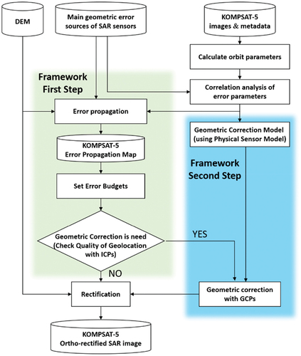
A schematic of this study is shown in Figure 1. First, the correlations between the main error sources were analyzed. Subsequently, based on the results of the correlation analysis, error propagation maps were generated using the law of variance propagation. Error propagation maps were used to set the error budget for the geocoding accuracy of SAR images. Then, a geometric correction model without multicollinearity was developed using the least squares method (LSM) and the correlation analysis results of the main error sources. Next, geometric correction using GCPs was performed to improve the geocoding accuracy of the SAR images. Finally, geometric rectification was performed to generate an ortho-rectified SAR image with improved geocoding accuracy.

Figure 1. Research framework to improve the geocoding accuracy of SAR imagery. First step: Setting the error budget and checking the geocoding quality. Second step: Geometric correction.

2.2 Observation error theory

Observations can be imperfect with errors arising from several sources. The observation error is the difference between the value of the observation and its true value and can be divided into two components: systematic and random errors (Taylor 1997). Systematic error is a consistent or proportional difference between the observed and true values. The random error is the probability difference between the observed and true values. Systematic errors follow physical laws and can, thus, be predicted and removed by following correct observation procedures. Random errors remain even after all systematic errors are removed from the observed values. In general, these are the result of human and instrument imperfections, and must be addressed via the laws of probability. Hence, it is generally assumed that the random errors follow a normal distribution.

The observations, including the systematic errors, are expressed by Equation (1)(1) $y=\mu +\beta +e$(1) , where $y$ is the observation, $\mu$ is the true value of the observation, $\beta$ is the systematic error, and $e$ is the random error. The mathematical relationship between the observation, true value, and error after the systematic error has been removed can be expressed by Equation (2)(2) $y=\mu +e$(2) .

(1) $y=\mu +\beta +e$(1)

(2) $y=\mu +e$(2)

2.3 Main geometric error sources of SAR sensors

Error sources that affect the geocoding accuracy of SAR imagery include satellite orbit errors, sensor instability, topographical effects, and atmospheric effects. These errors can be classified into orbit, sensor, and system external variables, as summarized in Table 1 (Curlander and McDonough 1991; Choi, Hong, and Sohn 2019; Hong et al. 2013).

Table 1. Classification of main geometric error sources of SAR sensors. Here, e denotes a random error and $\beta$ denotes a systematic error component.

Main error sources
Orbit information	Satellite position ($e_{sp\left(X\right)},e_{sp\left(Y\right)},e_{sp\left(Z\right)}$) Satellite velocity ($e_{sv\left(X\right)},e_{sv\left(Y\right)},e_{sv\left(Z\right)}$)
Sensor information	Clock drift ($e_t$) Electronic delay (${\beta }_{ED}+e_{ED}$)
System external variables	Atmospheric effect (${\beta }_R+e_R$) Earth movement ($e_{R_T\left(X\right)},e_{R_T\left(Y\right)},e_{R_T\left(Z\right)}$)

2.3.1 Orbit information

Satellite ephemeris, such as satellite position and velocity, are essential factors in SAR satellite imaging systems. Previously, many low-orbit satellites were equipped with a single-frequency GPS receiver owing to their high cost and susceptibility to technical difficulties. Accordingly, the orbit information obtained from the header file had a positional error of hundreds of meters (Choi, Hong, and Sohn 2019). In this case, the geometric correction models focused on positional adjustment of the SAR satellite imaging system. However, recently launched satellites, such as TerraSAR-X and KOMPSAT-5, are equipped with dual-frequency GPS receivers that can be used for precise orbit determination (POD) and can provide an orbital accuracy of up to centimeters (Hwang et al. 2011; Wermuth et al. 2012).

2.3.2 Sensor information

Sensor information errors significantly affect the pixel allocation accuracy of SAR imagery (Cumming and Wong 2005; Montenbruck, Gill, and Lutze 2002; Oliver and Quegan 2004). The clock drift represents the time difference between the satellite orbit information and the radar system. Clock drift causes direct errors in the azimuthal direction of SAR imagery in proportion to the pulse repetition frequency (PRF) (Breit et al. 2009; Eineder et al. 2001; Hong et al. 2017). As the satellite velocity increases, the calculated distance between the satellite and ground target becomes distorted, and eventually, clock drift causes errors in the slant range direction (Yang, Liu, and Wang 2014). Electronic delay is a hardware problem caused by radar echo sampling. Electronic delays mainly cause errors in SAR image coordinates in the slant range direction (Eineder et al. 2001; Shimada 2018).

2.3.3 System external variables

Atmospheric effects and earth movements can affect the pixel allocation accuracy of SAR image (Jehle et al. 2008; Schubert et al. 2009, 2012). The atmospheric effect indicates that various particles in the atmosphere delay radar signals. Depending on the atmospheric conditions and path length, this causes an error of 2–4 m in the slant range direction (Ager and Bresnahan 2009). Earth movement is caused by various phenomena, such as earth fluctuations and tides. Periodic fluctuations of the earth occur vertically up to 40 cm in the mid-latitudes, which may affect the geocoding accuracy of the SAR image coordinates (Schubert et al. 2012). The Earth tide is the displacement of the solid Earth’s surface caused by the gravity of the Moon and Sun. Earth tides cause ground target coordinate errors, which also affect the geocoding accuracy of SAR imagery (Schubert et al. 2012).

2.4 SAR satellite imaging geometry

The relationship between the coordinates of the SAR image pixels and those of the ground targets can be defined by range-Doppler equations in the SAR satellite system (Soumekh 1999). Equations (3)(3) $R(t)={\left[\left({\overrightarrow{P}}^S(t)-{\overrightarrow{P}}_T\right)\cdot \left({\overrightarrow{P}}^S(t)-{\overrightarrow{P}}_T\right)\right]}^{1/2}+({\beta }_R+e_R)-\mathrm{c}\times ({\beta }_{ED}+e_{ED})/2$(3) and (4(4) $f_{DC}(t)=\frac{2\left({\overrightarrow{V}}^S(t)-{\overrightarrow{V}}_T\right)\cdot \left({\overrightarrow{P}}^S(t)-{\overrightarrow{P}}_T\right)}{\lambda \left(\left|{\overrightarrow{P}}^S(t)-{\overrightarrow{P}}_T\right|+({\beta }_R+e_R)-\mathrm{c}\times ({\beta }_{ED}+e_{ED})/2\right)}$(4) ) can be derived by considering the random and systematic errors of electronic delay (${\beta }_{ED}+e_{ED}$) and atmospheric effects (${\beta }_R+e_R$) in the range-Doppler equations.

(3) $R(t)={\left[\left({\overrightarrow{P}}^S(t)-{\overrightarrow{P}}_T\right)\cdot \left({\overrightarrow{P}}^S(t)-{\overrightarrow{P}}_T\right)\right]}^{1/2}+({\beta }_R+e_R)-\mathrm{c}\times ({\beta }_{ED}+e_{ED})/2$(3)

(4) $f_{DC}(t)=\frac{2\left({\overrightarrow{V}}^S(t)-{\overrightarrow{V}}_T\right)\cdot \left({\overrightarrow{P}}^S(t)-{\overrightarrow{P}}_T\right)}{\lambda \left(\left|{\overrightarrow{P}}^S(t)-{\overrightarrow{P}}_T\right|+({\beta }_R+e_R)-\mathrm{c}\times ({\beta }_{ED}+e_{ED})/2\right)}$(4)

In Equations (3)(3) $R(t)={\left[\left({\overrightarrow{P}}^S(t)-{\overrightarrow{P}}_T\right)\cdot \left({\overrightarrow{P}}^S(t)-{\overrightarrow{P}}_T\right)\right]}^{1/2}+({\beta }_R+e_R)-\mathrm{c}\times ({\beta }_{ED}+e_{ED})/2$(3) and (4(4) $f_{DC}(t)=\frac{2\left({\overrightarrow{V}}^S(t)-{\overrightarrow{V}}_T\right)\cdot \left({\overrightarrow{P}}^S(t)-{\overrightarrow{P}}_T\right)}{\lambda \left(\left|{\overrightarrow{P}}^S(t)-{\overrightarrow{P}}_T\right|+({\beta }_R+e_R)-\mathrm{c}\times ({\beta }_{ED}+e_{ED})/2\right)}$(4) ), $\lambda$ is the wavelength of the signal, $\mathrm{c}$ is the speed of light, ${\vec{P}}_T$ is the coordinate of the ground target position, ${\vec{V}}_T$ is the velocity of the ground target, ${\vec{P}}^S\left(t\right)$ is the coordinate of the satellite position, and ${\vec{V}}^S\left(t\right)$ is the velocity of the satellite. In this study, $\lambda$ is used as the value specified in the header file of the input SAR image, and ${\vec{V}}_T$ is assumed to be 0. Equation (5)(5) ${\overrightarrow{P}}_T=\left[\begin{array}{c}{X}_T\\ Y_T\\ Z_T\end{array}\right]+\left[\begin{array}{c}{e}_{R_T(X)}\\ e_{R_T(Y)}\\ e_{R_T(Z)}\end{array}\right]$(5) is an expression for ${\vec{P}}_T$ that considers the earth movement errors ($e_{R_T\left(X\right)},e_{R_T\left(Y\right)},e_{R_T\left(Z\right)}$).

(5) ${\overrightarrow{P}}_T=\left[\begin{array}{c}{X}_T\\ Y_T\\ Z_T\end{array}\right]+\left[\begin{array}{c}{e}_{R_T(X)}\\ e_{R_T(Y)}\\ e_{R_T(Z)}\end{array}\right]$(5)

${\vec{P}}^S\left(t\right)$ and ${\vec{V}}^S\left(t\right)$ continuously change with time as satellite imagery is acquired. Therefore, time-dependent polynomial equations can be applied to satellite orbit models (Hong et al. 2017; Toutin 2004). In this study, the satellite position is defined by a second-order time-dependent equation, and Equation (6)(6) ${\overrightarrow{P}}^S(t)=\left[\begin{array}{c}{P_X}^S\\ {P_Y}^S\\ {P_Z}^S\end{array}\right]=\left[\begin{array}{c}{a}_0+a_{1}t+a_2{t}^2\\ b_0+b_{1}t+b_2{t}^2\\ c_0+c_{1}t+c_2{t}^2\end{array}\right]+\left[\begin{array}{c}{e}_{sp(X)}\\ e_{sp(Y)}\\ e_{sp(Z)}\end{array}\right]$(6) represents ${\vec{P}}^S\left(t\right)$ by considering the satellite position errors ($e_{sp\left(X\right)},e_{sp\left(Y\right)},e_{sp\left(Z\right)}$). The satellite velocity is defined as the time derivative of the satellite position vector, and Equation (7)(7) ${\overrightarrow{V}}^S(t)=\left[\begin{array}{c}{V_X}^S\\ {V_Y}^S\\ {V_Z}^S\end{array}\right]=\left[\begin{array}{c}{a}_1+2a_{2}t\\ b_1+2b_{2}t\\ c_1+2c_{2}t\end{array}\right]+\left[\begin{array}{c}{e}_{sv(X)}\\ e_{sv(Y)}\\ e_{sv(Z)}\end{array}\right]$(7) represents ${\vec{V}}^S\left(t\right)$ with satellite velocity errors ($e_{sv\left(X\right)},e_{sv\left(Y\right)},e_{sv\left(Z\right)}$).

(6) ${\overrightarrow{P}}^S(t)=\left[\begin{array}{c}{P_X}^S\\ {P_Y}^S\\ {P_Z}^S\end{array}\right]=\left[\begin{array}{c}{a}_0+a_{1}t+a_2{t}^2\\ b_0+b_{1}t+b_2{t}^2\\ c_0+c_{1}t+c_2{t}^2\end{array}\right]+\left[\begin{array}{c}{e}_{sp(X)}\\ e_{sp(Y)}\\ e_{sp(Z)}\end{array}\right]$(6)

(7) ${\overrightarrow{V}}^S(t)=\left[\begin{array}{c}{V_X}^S\\ {V_Y}^S\\ {V_Z}^S\end{array}\right]=\left[\begin{array}{c}{a}_1+2a_{2}t\\ b_1+2b_{2}t\\ c_1+2c_{2}t\end{array}\right]+\left[\begin{array}{c}{e}_{sv(X)}\\ e_{sv(Y)}\\ e_{sv(Z)}\end{array}\right]$(7)

In Equations (6)(6) ${\overrightarrow{P}}^S(t)=\left[\begin{array}{c}{P_X}^S\\ {P_Y}^S\\ {P_Z}^S\end{array}\right]=\left[\begin{array}{c}{a}_0+a_{1}t+a_2{t}^2\\ b_0+b_{1}t+b_2{t}^2\\ c_0+c_{1}t+c_2{t}^2\end{array}\right]+\left[\begin{array}{c}{e}_{sp(X)}\\ e_{sp(Y)}\\ e_{sp(Z)}\end{array}\right]$(6) and (7(7) ${\overrightarrow{V}}^S(t)=\left[\begin{array}{c}{V_X}^S\\ {V_Y}^S\\ {V_Z}^S\end{array}\right]=\left[\begin{array}{c}{a}_1+2a_{2}t\\ b_1+2b_{2}t\\ c_1+2c_{2}t\end{array}\right]+\left[\begin{array}{c}{e}_{sv(X)}\\ e_{sv(Y)}\\ e_{sv(Z)}\end{array}\right]$(7) ), $a_0,a_1,a_2,b_0,b_1,b_2,c_0,c_1,c_2$ are satellite orbital coefficients that can be estimated from the satellite ephemeris information provided in the header file of the SAR data (Hong et al. 2017). Because there are nine unknowns, at least two satellite orbit information points (position and velocity) are required. Therefore, LSM can be applied to estimate the satellite orbital coefficients from three points of satellite ephemeris information.

In the SAR satellite system, the sampling time for a ground target is the time at which the distance between the satellite and ground target is minimal. When the Doppler equation equals zero, the distance between the satellite and ground target is at its minimum (Equation (8)(8) $f(t)=\left({\overrightarrow{V}}^S(t)-{\overrightarrow{V}}_T\right)\cdot \left({\overrightarrow{P}}^S(t)-{\overrightarrow{P}}_T\right)=0$(8) ). Equation (8)(8) $f(t)=\left({\overrightarrow{V}}^S(t)-{\overrightarrow{V}}_T\right)\cdot \left({\overrightarrow{P}}^S(t)-{\overrightarrow{P}}_T\right)=0$(8) can be rearranged in the form of a cubic equation of time ($t$), as shown in Equation (9)(9) $\begin{array}{rl}& wherea=2{a_2}^2+2{b_2}^2+2{c_2}^2\\ & b=3a_1{a}_2+a_2{e}_{sv(X)}+3b_1{b}_2+b_2{e}_{sv(Y)}+3c_1{c}_2\\ & +c_2{e}_{sv(Z)}\\ & c=-2X_T{a}_2-2Y_T{b}_2-2Z_T{c}_2+2a_0{a}_2+{a_1}^2\\ & +a_1{e}_{sv(X)}-2a_2{e}_{R_T(X)}+2a_2{e}_{sp(X)}+2b_0{b}_2\\ & +{b_1}^2+b_1{e}_{sv(Y)}-2b_2{e}_{R_T(Y)}+2b_2{e}_{sp(Y)}\\ & +2c_0{c}_2+{c_1}^2+c_1{e}_{sv(Z)}-2c_2{e}_{R_T(Z)}\\ & +2c_2{e}_{sp(Z)}\\ & d=-X_T{a}_1-X_T{e}_{sv(X)}-Y_T{b}_1-Y_T{e}_{sv(Y)}-Z_T{c}_1\\ & -Z_T{e}_{sv(Z)}+a_0{a}_1+a_0{e}_{sv(X)}-a_1{e}_{R_T(X)}\\ & +a_1{e}_{sp(X)}+b_0{b}_1+b_0{e}_{sv(Y)}-b_1{e}_{R_T(Y)}\\ & +b_1{e}_{sp(Y)}+c_0{c}_1+c_0{e}_{sv(Z)}-c_1{e}_{R_T(Z)}\\ & +c_1{e}_{sp(Z)}-e_{R_T(X)}{e}_{sv(X)}-e_{R_T(Y)}{e}_{sv(Y)}\\ & -e_{R_T(Z)}{e}_{sv(Z)}+e_{sp(X)}{e}_{ev(X)}+e_{sp(Y)}{e}_{ev(Y)}\\ & +e_{sp(Z)}{e}_{ev(Z)}\end{array}$(9) , and time ($t$) can be described by Equation (10)(10) $\begin{array}{rl}& t=-\frac{b}{3a}-\frac{1}{3a}\sqrt[3]{\frac{2b^3-9abc+27a^{2}d+\sqrt{2b^3-9abc+27a^{2}d{)}^2-4{(b^2-3ac)}^3}}{2}}\\ & -\frac{1}{3a}\sqrt[3]{\frac{2b^3-9abc+27a^{2}d-\sqrt{2b^3-9abc+27a^{2}d{)}^2-4{(b^2-3ac)}^3}}{2}}\end{array}$(10) using Cardano’s method (Dunham 1990). $a,b,c,d$ are the coefficients of the cubic equation when the zero-Doppler equation is rearranged in the form of a cubic equation of time ($t$).

(8) $f(t)=\left({\overrightarrow{V}}^S(t)-{\overrightarrow{V}}_T\right)\cdot \left({\overrightarrow{P}}^S(t)-{\overrightarrow{P}}_T\right)=0$(8)

$a{t}^3+b{t}^2+ct+d=0$

(9) $\begin{array}{rl}& wherea=2{a_2}^2+2{b_2}^2+2{c_2}^2\\ & b=3a_1{a}_2+a_2{e}_{sv(X)}+3b_1{b}_2+b_2{e}_{sv(Y)}+3c_1{c}_2\\ & +c_2{e}_{sv(Z)}\\ & c=-2X_T{a}_2-2Y_T{b}_2-2Z_T{c}_2+2a_0{a}_2+{a_1}^2\\ & +a_1{e}_{sv(X)}-2a_2{e}_{R_T(X)}+2a_2{e}_{sp(X)}+2b_0{b}_2\\ & +{b_1}^2+b_1{e}_{sv(Y)}-2b_2{e}_{R_T(Y)}+2b_2{e}_{sp(Y)}\\ & +2c_0{c}_2+{c_1}^2+c_1{e}_{sv(Z)}-2c_2{e}_{R_T(Z)}\\ & +2c_2{e}_{sp(Z)}\\ & d=-X_T{a}_1-X_T{e}_{sv(X)}-Y_T{b}_1-Y_T{e}_{sv(Y)}-Z_T{c}_1\\ & -Z_T{e}_{sv(Z)}+a_0{a}_1+a_0{e}_{sv(X)}-a_1{e}_{R_T(X)}\\ & +a_1{e}_{sp(X)}+b_0{b}_1+b_0{e}_{sv(Y)}-b_1{e}_{R_T(Y)}\\ & +b_1{e}_{sp(Y)}+c_0{c}_1+c_0{e}_{sv(Z)}-c_1{e}_{R_T(Z)}\\ & +c_1{e}_{sp(Z)}-e_{R_T(X)}{e}_{sv(X)}-e_{R_T(Y)}{e}_{sv(Y)}\\ & -e_{R_T(Z)}{e}_{sv(Z)}+e_{sp(X)}{e}_{ev(X)}+e_{sp(Y)}{e}_{ev(Y)}\\ & +e_{sp(Z)}{e}_{ev(Z)}\end{array}$(9)

(10) $\begin{array}{rl}& t=-\frac{b}{3a}-\frac{1}{3a}\sqrt[3]{\frac{2b^3-9abc+27a^{2}d+\sqrt{2b^3-9abc+27a^{2}d{)}^2-4{(b^2-3ac)}^3}}{2}}\\ & -\frac{1}{3a}\sqrt[3]{\frac{2b^3-9abc+27a^{2}d-\sqrt{2b^3-9abc+27a^{2}d{)}^2-4{(b^2-3ac)}^3}}{2}}\end{array}$(10)

The azimuth pixel coordinate ($i$) and range pixel coordinate ($j$) of the SAR image can be expressed as equations for the sampling time of a ground target. Equation (11)(11) $i=f_i\left(t\right)=\frac{\left(t+e_t\right)-t_0}{1/PRF},j=f_j\left(t\right)=\frac{2\times \left(R\left(t+e_t\right)-R_0\right)}{\mathrm{c}/RSF}$(11) is the coordinate equations of a SAR image pixel with a clock drift error ($e_t$). The SAR image pixel coordinates can be expressed as equations for the ground target position and error sources by substituting Equation (10)(10) $\begin{array}{rl}& t=-\frac{b}{3a}-\frac{1}{3a}\sqrt[3]{\frac{2b^3-9abc+27a^{2}d+\sqrt{2b^3-9abc+27a^{2}d{)}^2-4{(b^2-3ac)}^3}}{2}}\\ & -\frac{1}{3a}\sqrt[3]{\frac{2b^3-9abc+27a^{2}d-\sqrt{2b^3-9abc+27a^{2}d{)}^2-4{(b^2-3ac)}^3}}{2}}\end{array}$(10) into Equation (11)(11) $i=f_i\left(t\right)=\frac{\left(t+e_t\right)-t_0}{1/PRF},j=f_j\left(t\right)=\frac{2\times \left(R\left(t+e_t\right)-R_0\right)}{\mathrm{c}/RSF}$(11) , as shown in Equation (12)(12) $\begin{array}{rl}& i=f_{i\mathrm{\_}e\mathrm{\_}t}(X_T,Y_T,Z_T,e_{sp(X)},e_{sp(Y)},e_{sp(Z)},e_{sv(X)},e_{sv(Y)},\\ & e_{sv(Z)},e_t,{\beta }_{ED}+e_{ED},{\beta }_R+e_R,e_{R_T(X)},e_{R_T(Y)},e_{R_T(Z)})\\ & j=f_{j\mathrm{\_}e\mathrm{\_}t}(X_T,Y_T,Z_T,e_{sp(X)},e_{sp(Y)},e_{sp(Z)},e_{sv(X)},e_{sv(Y)},\\ & e_{sv(Z)},e_t,{\beta }_{ED}+e_{ED},{\beta }_R+e_R,e_{R_T(X)},e_{R_T(Y)},e_{R_T(Z)})\end{array}$(12) . $t_0$ is the imaging start time, $PRF$ is the pulse repetition frequency, $RSF$ is the range sampling frequency, and $R_0$ is the distance from the column direction to the first pixel.

(11) $i=f_i\left(t\right)=\frac{\left(t+e_t\right)-t_0}{1/PRF},j=f_j\left(t\right)=\frac{2\times \left(R\left(t+e_t\right)-R_0\right)}{\mathrm{c}/RSF}$(11)

(12) $\begin{array}{rl}& i=f_{i\mathrm{\_}e\mathrm{\_}t}(X_T,Y_T,Z_T,e_{sp(X)},e_{sp(Y)},e_{sp(Z)},e_{sv(X)},e_{sv(Y)},\\ & e_{sv(Z)},e_t,{\beta }_{ED}+e_{ED},{\beta }_R+e_R,e_{R_T(X)},e_{R_T(Y)},e_{R_T(Z)})\\ & j=f_{j\mathrm{\_}e\mathrm{\_}t}(X_T,Y_T,Z_T,e_{sp(X)},e_{sp(Y)},e_{sp(Z)},e_{sv(X)},e_{sv(Y)},\\ & e_{sv(Z)},e_t,{\beta }_{ED}+e_{ED},{\beta }_R+e_R,e_{R_T(X)},e_{R_T(Y)},e_{R_T(Z)})\end{array}$(12)

Previous studies on SAR satellite imaging geometry mostly applied the Newton–Raphson method to calculate the time ($t$) through an iterative calculation process and substituted the final time ($t$) into the equations of a SAR image pixel to calculate the coordinates of the corresponding pixel. This approach requires two steps to compute the coordinates of the SAR image pixel. However, in this study, we implemented a direct method that calculates the coordinates of SAR image pixels without an iterative process by applying Cardano’s method. An advantage of Cardano’s method is that it allows us to define the SAR image pixel coordinate equations with the ground target position and error sources as variables, as indicated in Equation (12)(12) $\begin{array}{rl}& i=f_{i\mathrm{\_}e\mathrm{\_}t}(X_T,Y_T,Z_T,e_{sp(X)},e_{sp(Y)},e_{sp(Z)},e_{sv(X)},e_{sv(Y)},\\ & e_{sv(Z)},e_t,{\beta }_{ED}+e_{ED},{\beta }_R+e_R,e_{R_T(X)},e_{R_T(Y)},e_{R_T(Z)})\\ & j=f_{j\mathrm{\_}e\mathrm{\_}t}(X_T,Y_T,Z_T,e_{sp(X)},e_{sp(Y)},e_{sp(Z)},e_{sv(X)},e_{sv(Y)},\\ & e_{sv(Z)},e_t,{\beta }_{ED}+e_{ED},{\beta }_R+e_R,e_{R_T(X)},e_{R_T(Y)},e_{R_T(Z)})\end{array}$(12) . Furthermore, this enables us to calculate the correlations among error sources, check how much errors propagate to the coordinates of SAR image pixels, and develop a geometric correction model that can directly calculate the coordinates of SAR image pixels with improved geocoding accuracy.

2.5 Error budget of SAR geocoding

The main geometric error sources of the SAR sensors were reviewed in Section 2.3. These errors can be classified as systematic or random. Among these, satellite position errors ($e_{sp\left(X\right)},e_{sp\left(Y\right)},e_{sp\left(Z\right)}$), satellite velocity errors ($e_{sv\left(X\right)},e_{sv\left(Y\right)},e_{sv\left(Z\right)}$), clock drift error ($e_t$), and earth movement errors ($e_{R_T\left(X\right)},e_{R_T\left(Y\right)},e_{R_T\left(Z\right)}$) were assumed to be random errors, and electronic delay error (${\beta }_{ED}+e_{ED}$) and atmospheric effects error (${\beta }_R+e_R$) were assumed to be combinations of systematic and random errors, according to previous studies (Ager and Bresnahan 2009; Breit et al. 2009; Choi, Hong, and Sohn 2019; Eineder et al. 2001, 2010; Hong et al. 2013; Hwang et al. 2011; Jehle et al. 2008; Schubert et al. 2009, 2012).

Systematic errors can be removed by subtracting biased values; however, random errors can not be eliminated because of their random nature. Thus, random errors are propagated to the final coordinates of the SAR image pixels. To easily identify the influence of random errors on the geocoding accuracy of SAR satellite imagery, error propagation maps were generated using the law of variance propagation (Equation (13)(13) ${\sum }_{i,j}=J{\sum }_{randomerrors}{J}^T$(13) ) (Kim et al. 2020). The error propagation results were then double-checked using a Monte Carlo simulation. The Jacobian matrix $\left(J\right)$ in Equation (13)(13) ${\sum }_{i,j}=J{\sum }_{randomerrors}{J}^T$(13) can be calculated as shown in Equation (14)(14) $J=\left[\begin{array}{cccccccccccc}\frac{\mathrm{\partial }{f}_{i\mathrm{\_}e\mathrm{\_}t}}{\mathrm{\partial }{e}_{sp(X)}}& \frac{\mathrm{\partial }{f}_{i\mathrm{\_}e\mathrm{\_}t}}{\mathrm{\partial }{e}_{sp(Y)}}& \frac{\mathrm{\partial }{f}_{i\mathrm{\_}e\mathrm{\_}t}}{\mathrm{\partial }{e}_{sp(Z)}}& \frac{\mathrm{\partial }{f}_{i\mathrm{\_}e\mathrm{\_}t}}{\mathrm{\partial }{e}_{sv(X)}}& \frac{\mathrm{\partial }{f}_{i\mathrm{\_}e\mathrm{\_}t}}{\mathrm{\partial }{e}_{sv(Y)}}& \frac{\mathrm{\partial }{f}_{i\mathrm{\_}e\mathrm{\_}t}}{\mathrm{\partial }{e}_{sv(Z)}}& \frac{\mathrm{\partial }{f}_{i\mathrm{\_}e\mathrm{\_}t}}{\mathrm{\partial }{e}_t}& \frac{\mathrm{\partial }{f}_{i\mathrm{\_}e\mathrm{\_}t}}{\mathrm{\partial }{e}_{ED}}& \frac{\mathrm{\partial }{f}_{i\mathrm{\_}e\mathrm{\_}t}}{\mathrm{\partial }{e}_R}& \frac{\mathrm{\partial }{f}_{i\mathrm{\_}e\mathrm{\_}t}}{\mathrm{\partial }{e}_{R_T(X)}}& \frac{\mathrm{\partial }{f}_{i\mathrm{\_}e\mathrm{\_}t}}{\mathrm{\partial }{e}_{R_T(Y)}}& \frac{\mathrm{\partial }{f}_{i\mathrm{\_}e\mathrm{\_}t}}{\mathrm{\partial }{e}_{R_T(Z)}}\\ \frac{\mathrm{\partial }{f}_{j\mathrm{\_}e\mathrm{\_}t}}{\mathrm{\partial }{e}_{sp(X)}}& \frac{\mathrm{\partial }{f}_{j\mathrm{\_}e\mathrm{\_}t}}{\mathrm{\partial }{e}_{sp(Y)}}& \frac{\mathrm{\partial }{f}_{j\mathrm{\_}e\mathrm{\_}t}}{\mathrm{\partial }{e}_{sp(Z)}}& \frac{\mathrm{\partial }{f}_{j\mathrm{\_}e\mathrm{\_}t}}{\mathrm{\partial }{e}_{sv(X)}}& \frac{\mathrm{\partial }{f}_{j\mathrm{\_}e\mathrm{\_}t}}{\mathrm{\partial }{e}_{sv(Y)}}& \frac{\mathrm{\partial }{f}_{j\mathrm{\_}e\mathrm{\_}t}}{\mathrm{\partial }{e}_{sv(Z)}}& \frac{\mathrm{\partial }{f}_{j\mathrm{\_}e\mathrm{\_}t}}{\mathrm{\partial }{e}_t}& \frac{\mathrm{\partial }{f}_{j\mathrm{\_}e\mathrm{\_}t}}{\mathrm{\partial }{e}_{ED}}& \frac{\mathrm{\partial }{f}_{j\mathrm{\_}e\mathrm{\_}t}}{\mathrm{\partial }{e}_R}& \frac{\mathrm{\partial }{f}_{j\mathrm{\_}e\mathrm{\_}t}}{\mathrm{\partial }{e}_{R_T(X)}}& \frac{\mathrm{\partial }{f}_{j\mathrm{\_}e\mathrm{\_}t}}{\mathrm{\partial }{e}_{R_T(Y)}}& \frac{\mathrm{\partial }{f}_{j\mathrm{\_}e\mathrm{\_}t}}{\mathrm{\partial }{e}_{R_T(Z)}}\end{array}\right]$(14) by the partial differentiation of Equation (12)(12) $\begin{array}{rl}& i=f_{i\mathrm{\_}e\mathrm{\_}t}(X_T,Y_T,Z_T,e_{sp(X)},e_{sp(Y)},e_{sp(Z)},e_{sv(X)},e_{sv(Y)},\\ & e_{sv(Z)},e_t,{\beta }_{ED}+e_{ED},{\beta }_R+e_R,e_{R_T(X)},e_{R_T(Y)},e_{R_T(Z)})\\ & j=f_{j\mathrm{\_}e\mathrm{\_}t}(X_T,Y_T,Z_T,e_{sp(X)},e_{sp(Y)},e_{sp(Z)},e_{sv(X)},e_{sv(Y)},\\ & e_{sv(Z)},e_t,{\beta }_{ED}+e_{ED},{\beta }_R+e_R,e_{R_T(X)},e_{R_T(Y)},e_{R_T(Z)})\end{array}$(12) with respect to random errors, where ${\sum }_{randomerrors}$ is a dispersion matrix of random errors. In this case, it is important to consider the correlations among random errors. The detailed methods and results of the correlation analysis are described in Section 4.1.

(13) ${\sum }_{i,j}=J{\sum }_{randomerrors}{J}^T$(13)

(14) $J=\left[\begin{array}{cccccccccccc}\frac{\mathrm{\partial }{f}_{i\mathrm{\_}e\mathrm{\_}t}}{\mathrm{\partial }{e}_{sp(X)}}& \frac{\mathrm{\partial }{f}_{i\mathrm{\_}e\mathrm{\_}t}}{\mathrm{\partial }{e}_{sp(Y)}}& \frac{\mathrm{\partial }{f}_{i\mathrm{\_}e\mathrm{\_}t}}{\mathrm{\partial }{e}_{sp(Z)}}& \frac{\mathrm{\partial }{f}_{i\mathrm{\_}e\mathrm{\_}t}}{\mathrm{\partial }{e}_{sv(X)}}& \frac{\mathrm{\partial }{f}_{i\mathrm{\_}e\mathrm{\_}t}}{\mathrm{\partial }{e}_{sv(Y)}}& \frac{\mathrm{\partial }{f}_{i\mathrm{\_}e\mathrm{\_}t}}{\mathrm{\partial }{e}_{sv(Z)}}& \frac{\mathrm{\partial }{f}_{i\mathrm{\_}e\mathrm{\_}t}}{\mathrm{\partial }{e}_t}& \frac{\mathrm{\partial }{f}_{i\mathrm{\_}e\mathrm{\_}t}}{\mathrm{\partial }{e}_{ED}}& \frac{\mathrm{\partial }{f}_{i\mathrm{\_}e\mathrm{\_}t}}{\mathrm{\partial }{e}_R}& \frac{\mathrm{\partial }{f}_{i\mathrm{\_}e\mathrm{\_}t}}{\mathrm{\partial }{e}_{R_T(X)}}& \frac{\mathrm{\partial }{f}_{i\mathrm{\_}e\mathrm{\_}t}}{\mathrm{\partial }{e}_{R_T(Y)}}& \frac{\mathrm{\partial }{f}_{i\mathrm{\_}e\mathrm{\_}t}}{\mathrm{\partial }{e}_{R_T(Z)}}\\ \frac{\mathrm{\partial }{f}_{j\mathrm{\_}e\mathrm{\_}t}}{\mathrm{\partial }{e}_{sp(X)}}& \frac{\mathrm{\partial }{f}_{j\mathrm{\_}e\mathrm{\_}t}}{\mathrm{\partial }{e}_{sp(Y)}}& \frac{\mathrm{\partial }{f}_{j\mathrm{\_}e\mathrm{\_}t}}{\mathrm{\partial }{e}_{sp(Z)}}& \frac{\mathrm{\partial }{f}_{j\mathrm{\_}e\mathrm{\_}t}}{\mathrm{\partial }{e}_{sv(X)}}& \frac{\mathrm{\partial }{f}_{j\mathrm{\_}e\mathrm{\_}t}}{\mathrm{\partial }{e}_{sv(Y)}}& \frac{\mathrm{\partial }{f}_{j\mathrm{\_}e\mathrm{\_}t}}{\mathrm{\partial }{e}_{sv(Z)}}& \frac{\mathrm{\partial }{f}_{j\mathrm{\_}e\mathrm{\_}t}}{\mathrm{\partial }{e}_t}& \frac{\mathrm{\partial }{f}_{j\mathrm{\_}e\mathrm{\_}t}}{\mathrm{\partial }{e}_{ED}}& \frac{\mathrm{\partial }{f}_{j\mathrm{\_}e\mathrm{\_}t}}{\mathrm{\partial }{e}_R}& \frac{\mathrm{\partial }{f}_{j\mathrm{\_}e\mathrm{\_}t}}{\mathrm{\partial }{e}_{R_T(X)}}& \frac{\mathrm{\partial }{f}_{j\mathrm{\_}e\mathrm{\_}t}}{\mathrm{\partial }{e}_{R_T(Y)}}& \frac{\mathrm{\partial }{f}_{j\mathrm{\_}e\mathrm{\_}t}}{\mathrm{\partial }{e}_{R_T(Z)}}\end{array}\right]$(14)

2.6 Quality improvement of SAR geocoding

Quality improvement of the SAR geocoding accuracy can be implemented using GCP-based geometric correction. A GCP-based geometric correction model using PSM can be developed by mathematically defining the physical relationship between the coordinates of ground targets and SAR image pixels. The least squares solution (LESS) can be obtained by minimizing the discrepancy between the image and ground coordinates using GCPs (Ghilani 2017; Koch 1999). The error sources in the observed values must be parameterized to set up a geometric correction model using the PSM (Toutin 2004). Equation (15)(15) $\begin{array}{rl}& i=f_{i\mathrm{\_}e\mathrm{\_}p12}(X_T,Y_T,Z_T,p_{sp(X)},p_{sp(Y)},p_{sp(Z)},p_{sv(X)},\\ & p_{sv(Y)},p_{sv(Z)},p_t,p_{ED},p_R,p_{R_T(X)},p_{R_T(Y)},p_{R_T(Z)})\\ & j=f_{j\mathrm{\_}e\mathrm{\_}p12}(X_T,Y_T,Z_T,p_{sp(X)},p_{sp(Y)},p_{sp(Z)},p_{sv(X)},\\ & p_{sv(Y)},p_{sv(Z)},p_t,p_{ED},p_R,p_{R_T(X)},p_{R_T(Y)},p_{R_T(Z)})\end{array}$(15) can be defined by replacing the satellite position errors ($e_{sp\left(X\right)},e_{sp\left(Y\right)},e_{sp\left(Z\right)}$), satellite velocity errors ($e_{sv\left(X\right)},e_{sv\left(Y\right)},e_{sv\left(Z\right)}$), clock drift error ($e_t$), electronic delay error (${\beta }_{ED}+e_{ED}$), atmospheric effect error (${\beta }_R+e_R$), and earth movement errors ($e_{R_T\left(X\right)},e_{R_T\left(Y\right)},e_{R_T\left(Z\right)}$) in Equation (12)(12) $\begin{array}{rl}& i=f_{i\mathrm{\_}e\mathrm{\_}t}(X_T,Y_T,Z_T,e_{sp(X)},e_{sp(Y)},e_{sp(Z)},e_{sv(X)},e_{sv(Y)},\\ & e_{sv(Z)},e_t,{\beta }_{ED}+e_{ED},{\beta }_R+e_R,e_{R_T(X)},e_{R_T(Y)},e_{R_T(Z)})\\ & j=f_{j\mathrm{\_}e\mathrm{\_}t}(X_T,Y_T,Z_T,e_{sp(X)},e_{sp(Y)},e_{sp(Z)},e_{sv(X)},e_{sv(Y)},\\ & e_{sv(Z)},e_t,{\beta }_{ED}+e_{ED},{\beta }_R+e_R,e_{R_T(X)},e_{R_T(Y)},e_{R_T(Z)})\end{array}$(12) with error parameters ($p_{sp\left(X\right)},p_{sp\left(Y\right)},p_{sp\left(Z\right)},$ $p_{sv\left(X\right)},p_{sv\left(Y\right)},p_{sv\left(Z\right)},$ $p_t,p_{ED},p_R,$ $p_{R_T\left(X\right)},p_{R_T\left(Y\right)},p_{R_T\left(Z\right)}$).

(15) $\begin{array}{rl}& i=f_{i\mathrm{\_}e\mathrm{\_}p12}(X_T,Y_T,Z_T,p_{sp(X)},p_{sp(Y)},p_{sp(Z)},p_{sv(X)},\\ & p_{sv(Y)},p_{sv(Z)},p_t,p_{ED},p_R,p_{R_T(X)},p_{R_T(Y)},p_{R_T(Z)})\\ & j=f_{j\mathrm{\_}e\mathrm{\_}p12}(X_T,Y_T,Z_T,p_{sp(X)},p_{sp(Y)},p_{sp(Z)},p_{sv(X)},\\ & p_{sv(Y)},p_{sv(Z)},p_t,p_{ED},p_R,p_{R_T(X)},p_{R_T(Y)},p_{R_T(Z)})\end{array}$(15)

Equation (15)(15) $\begin{array}{rl}& i=f_{i\mathrm{\_}e\mathrm{\_}p12}(X_T,Y_T,Z_T,p_{sp(X)},p_{sp(Y)},p_{sp(Z)},p_{sv(X)},\\ & p_{sv(Y)},p_{sv(Z)},p_t,p_{ED},p_R,p_{R_T(X)},p_{R_T(Y)},p_{R_T(Z)})\\ & j=f_{j\mathrm{\_}e\mathrm{\_}p12}(X_T,Y_T,Z_T,p_{sp(X)},p_{sp(Y)},p_{sp(Z)},p_{sv(X)},\\ & p_{sv(Y)},p_{sv(Z)},p_t,p_{ED},p_R,p_{R_T(X)},p_{R_T(Y)},p_{R_T(Z)})\end{array}$(15) is nonlinear with respect to error parameters. It is possible to develop a geometric correction model with 12 error parameters by estimating the error parameters through iterative calculations using a nonlinear Gauss–Markov model (GMM) (Ghilani 2017). However, multicollinearity in the model should be removed by parameter combination and feature selection because strong correlations among the parameters can cause an incorrect final solution in the LESS (Belsley, Kuh, and Welsch 2005; Shafizadeh-Moghadam et al. 2020). In this study, we analyzed the correlations between the error parameters and developed a geometric correction model without multicollinearity. The detailed methods and results for removing multicollinearity are described in Section 4.3.

3. Materials

3.1 KOMPSAT-5 SAR satellite images

KOMPSAT-5 is Korea’s first X-band SAR satellite system launched in 2013. In this study, two KOMPSAT-5 SAR satellite images from Daejeon, Korea, were used. The elevation of the study area is 50–450 m and includes various types of land cover, such as urban, rural, mountainous, and water. Table 2 summarizes the specifications of the SAR images used in the study.

Table 2. Basic information of KOMPSAT-5 SAR satellite images used in the study.

	SAR image #1	SAR image #2
Imaging mode	Enhanced High Resolution	High Resolution
Incidence angle	20.50° – 21.04°	53.91° – 54.15°
Orbit direction	Descending	Ascending
Look side	Right
Wavelength	0.031 m (X-band)
PRF	3.9308 × 10^3 Hz	3.4916 × 10^3 Hz
Projected spacing (Azimuth×Range)	0.63 m × 0.47 m	0.65 m × 1.44 m
Image size (Azimuth×Range)	8022 × 4070	7805 × 2906
Acquisition date	8 January 2016	18 December 2015
Product level	Level 1A

3.2 Digital elevation model (DEM) and aerial orthoimage

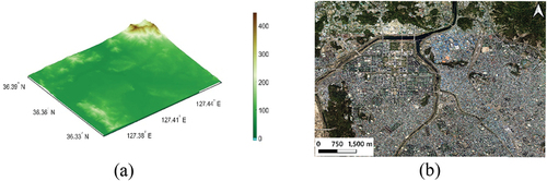
A digital elevation model (DEM) is required to generate ortho-rectified SAR images and error propagation maps. The quality of the DEM significantly affects the final ortho-rectified SAR images (Loew and Mauser 2007). The DEM with a 5 m spatial resolution is provided by the National Geographic Information Institute (NGII) of Korea. This is the best quality DEM that can be easily obtained; therefore, we utilized this in the experiments (Figure 2). High-resolution aerial orthoimages are also required to obtain accurate longitude and latitude coordinates of GCPs and independent check points (ICPs) for SAR image geometric correction. An aerial orthoimage with a 25 cm spatial resolution provided by NGII of Korea was utilized in the experiments (Figure 2). According to the digital map work regulations of Korea, the horizontal accuracy of an orthoimage is approximately 3.5 m.

Figure 2. DEM and aerial orthoimage of the study area: (a) DEM and (b) Aerial orthoimage.

3.3 Ground control points (GCPs) and independent check points (ICPs)

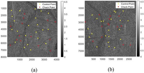
GCPs are required for geometric correction of SAR images. The role of ICPs is to evaluate geometric correction performance. The GCPs and ICPs were manually acquired using DEM and high-resolution aerial orthoimage. 22 GCPs and 14 ICPs were obtained for each SAR image. Figure 3 shows that GCPs and ICPs were evenly distributed throughout the study area.

Figure 3. GCPs and ICPs: (a) SAR image #1 and (b) SAR image #2.

3.4 Values of the random errors for generating error propagation maps

In this study, the random error values for generating error propagation maps were predetermined, as listed in Table 3, based on the results of previous studies on KOMPSAT-5 and TerraSAR-X, which are SAR satellites that use the X-band. (Ager and Bresnahan 2009; Breit et al. 2009; Choi, Hong, and Sohn 2019; Eineder et al. 2001, 2010; Hong et al. 2013; Hwang et al. 2011; Jehle et al. 2008; Schubert et al. 2009, 2012).

Table 3. Simulated values of the random errors affecting SAR geocoding accuracy. Simulated values were predetermined based on the results of previous studies.

Main error sources		Random errors
Orbit information	Satellite position Satellite velocity	$e_{sp\left(X\right)},e_{sp\left(Y\right)},e_{sp\left(Z\right)}=\pm 20cm$ $e_{sv\left(X\right)},e_{sv\left(Y\right)},e_{sv\left(Z\right)}=\pm 0.03cm/s$
Sensor information	Clock drift Electronic delay	$e_t=\pm 100\mu sec$ $e_{ED}=\pm 10nsec$
System external variables	Atmospheric effect	$e_R=\pm 1m$
	Earth movement	$e_{R_T\left(X\right)},e_{R_T\left(Y\right)}=\pm 0.1m$, $e_{R_T\left(Z\right)}=\pm 0.3m$

4. Results and discussions

4.1 Correlation analysis of main error sources

A correlation analysis of the main error sources can be performed using the geometric correction model with the 12 error parameters defined in Section 2.6. However, the geometric correction model with the 12 error parameters did not function normally because parameters with a correlation coefficient of 1 are present, prohibiting the values of these parameters from being estimated. Therefore, a step is required to combine parameters with a correlation coefficient of 1 into one parameter.

The correlation coefficient between the atmospheric effect error parameter ($p_R$) and electronic delay error parameter ($p_{ED}$) becomes 1. Additionally, the correlation coefficient between the satellite position error parameters ($p_{sp\left(X\right)},p_{sp\left(Y\right)},p_{sp\left(Z\right)}$) and earth movement error parameters ($p_{R_T\left(X\right)},p_{R_T\left(Y\right)},p_{R_T\left(Z\right)}$) also becomes 1. Both pairs of errors are parameterized at the same location with only different signs and scales within Equation (15)(15) $\begin{array}{rl}& i=f_{i\mathrm{\_}e\mathrm{\_}p12}(X_T,Y_T,Z_T,p_{sp(X)},p_{sp(Y)},p_{sp(Z)},p_{sv(X)},\\ & p_{sv(Y)},p_{sv(Z)},p_t,p_{ED},p_R,p_{R_T(X)},p_{R_T(Y)},p_{R_T(Z)})\\ & j=f_{j\mathrm{\_}e\mathrm{\_}p12}(X_T,Y_T,Z_T,p_{sp(X)},p_{sp(Y)},p_{sp(Z)},p_{sv(X)},\\ & p_{sv(Y)},p_{sv(Z)},p_t,p_{ED},p_R,p_{R_T(X)},p_{R_T(Y)},p_{R_T(Z)})\end{array}$(15) . When a pair of parameters is located in the same location with different scales and signs in the equations, that pair has a linear relationship. Therefore, their correlation coefficient is 1; hence, estimating the parameters using the least squares method is unreliable. A pair of parameters with a correlation coefficient of 1 must be combined into one parameter.

Equation (16)(16) $\begin{array}{cc}\hspace{0.17em}& i=f_{i\mathrm{\_}e\mathrm{\_}p8}(X_T,Y_T,Z_T,p_{sp,R_T\left(X\right)},p_{sp,R_T\left(Y\right)},p_{sp,R_T\left(Z\right)},\\ \hspace{0.17em}& p_{sv\left(X\right)},p_{sv\left(Y\right)},p_{sv\left(Z\right)},p_t,p_{ED,R})\\ \hspace{0.17em}& j=f_{j\mathrm{\_}e\mathrm{\_}p8}(X_T,Y_T,Z_T,p_{sp,R_T\left(X\right)},p_{sp,R_T\left(Y\right)},p_{sp,R_T\left(Z\right)},\\ \hspace{0.17em}& p_{sv\left(X\right)},p_{sv\left(Y\right)},p_{sv\left(Z\right)},p_t,p_{ED,R})\end{array}$(16) was defined by replacing “$p_R-\mathrm{c}\times p_{ED}/2$” with atmospheric and electronic delay error parameter ($p_{ED,R}$), replacing “${\left[\begin{array}{ccc}{p}_{sp\left(X\right)}& p_{sp\left(Y\right)}& p_{sp\left(Z\right)}\end{array}\right]}^T-{\left[\begin{array}{ccc}{p}_{R_T\left(X\right)}& p_{R_T\left(Y\right)}& p_{R_T\left(Z\right)}\end{array}\right]}^T$” with the satellite position and earth movement error parameters (${\left[\begin{array}{ccc}{p}_{sp,R_T\left(X\right)}& p_{sp,R_T\left(Y\right)}& p_{sp,R_T\left(Z\right)}\end{array}\right]}^T$). The geometric correction model can be redefined into eight error parameters using Equation (16)(16) $\begin{array}{cc}\hspace{0.17em}& i=f_{i\mathrm{\_}e\mathrm{\_}p8}(X_T,Y_T,Z_T,p_{sp,R_T\left(X\right)},p_{sp,R_T\left(Y\right)},p_{sp,R_T\left(Z\right)},\\ \hspace{0.17em}& p_{sv\left(X\right)},p_{sv\left(Y\right)},p_{sv\left(Z\right)},p_t,p_{ED,R})\\ \hspace{0.17em}& j=f_{j\mathrm{\_}e\mathrm{\_}p8}(X_T,Y_T,Z_T,p_{sp,R_T\left(X\right)},p_{sp,R_T\left(Y\right)},p_{sp,R_T\left(Z\right)},\\ \hspace{0.17em}& p_{sv\left(X\right)},p_{sv\left(Y\right)},p_{sv\left(Z\right)},p_t,p_{ED,R})\end{array}$(16) .

(16) $\begin{array}{cc}\hspace{0.17em}& i=f_{i\mathrm{\_}e\mathrm{\_}p8}(X_T,Y_T,Z_T,p_{sp,R_T\left(X\right)},p_{sp,R_T\left(Y\right)},p_{sp,R_T\left(Z\right)},\\ \hspace{0.17em}& p_{sv\left(X\right)},p_{sv\left(Y\right)},p_{sv\left(Z\right)},p_t,p_{ED,R})\\ \hspace{0.17em}& j=f_{j\mathrm{\_}e\mathrm{\_}p8}(X_T,Y_T,Z_T,p_{sp,R_T\left(X\right)},p_{sp,R_T\left(Y\right)},p_{sp,R_T\left(Z\right)},\\ \hspace{0.17em}& p_{sv\left(X\right)},p_{sv\left(Y\right)},p_{sv\left(Z\right)},p_t,p_{ED,R})\end{array}$(16)

The correlations among the eight error parameters can be analyzed by deriving the dispersion matrix using Equation (17)(17) $D\left\{\xi \right\}={{\sigma }_0}^2(A^{T}PA{)}^{-1}$(17) . ${{\sigma }_0}^2$ is the reference variance that can be calculated using Equation (18)(18) ${{\sigma }_o}^2\approx {{\hat{\sigma }}_o}^2=\frac{{\tilde{e}}^{T}P\tilde{e}}{2n-rkA}$(18) , where $\hat{\xi }$ and $\tilde{e}$ can be calculated using Equation (19)(20) $\tilde{e}=Y-f({\hat{\xi }}_{final})$(20) and (20(20) $\tilde{e}=Y-f({\hat{\xi }}_{final})$(20) ). The initial value of $\hat{\xi }$ is set to a zero vector. $n$ is number of GCPs. $Y$ is the column vector of observations, which are the pixel coordinates of the GCPs in the SAR image. $\xi$ is the column vector of eight error parameters. $A$ is a Jacobian matrix obtained by partial differentiation of Equation (16)(16) $\begin{array}{cc}\hspace{0.17em}& i=f_{i\mathrm{\_}e\mathrm{\_}p8}(X_T,Y_T,Z_T,p_{sp,R_T\left(X\right)},p_{sp,R_T\left(Y\right)},p_{sp,R_T\left(Z\right)},\\ \hspace{0.17em}& p_{sv\left(X\right)},p_{sv\left(Y\right)},p_{sv\left(Z\right)},p_t,p_{ED,R})\\ \hspace{0.17em}& j=f_{j\mathrm{\_}e\mathrm{\_}p8}(X_T,Y_T,Z_T,p_{sp,R_T\left(X\right)},p_{sp,R_T\left(Y\right)},p_{sp,R_T\left(Z\right)},\\ \hspace{0.17em}& p_{sv\left(X\right)},p_{sv\left(Y\right)},p_{sv\left(Z\right)},p_t,p_{ED,R})\end{array}$(16) with respect to the eight error parameters, and $P$ is the weight matrix of the observations. When acquiring GCPs manually, it was assumed that the probability of error occurrence in the GCPs of the SAR image was the same every time in the row and column directions; therefore, the same weight was assigned to all observations. Hence, the weight matrix is an identity matrix. The covariance and variance of the parameters can be found in the dispersion matrix, and the correlation coefficients of the parameters can be calculated by substituting the covariance and variance of the parameters into Equation (21)(21) ${\rho }_{XY}=\frac{cov(X,Y)}{{\sigma }_X{\sigma }_Y}$(21) . Figure 4 shows the absolute values of the correlation coefficients of the eight error parameters for SAR images #1 and #2 rounded to the fourth decimal place.

Figure 4. Correlation coefficients of the eight error parameters. Except for $p_t$, the correlations between the other parameters were calculated to be very high. Multicollinearity should be removed: (a) SAR image #1 and (b) SAR image #2.

(17) $D\left\{\xi \right\}={{\sigma }_0}^2(A^{T}PA{)}^{-1}$(17)

(18) ${{\sigma }_o}^2\approx {{\hat{\sigma }}_o}^2=\frac{{\tilde{e}}^{T}P\tilde{e}}{2n-rkA}$(18)

${\hat{\xi }}_n={\hat{\xi }}_{n-1}+\mathrm{\Delta }{\hat{\xi }}_{n}iterateuntil\mathrm{\Delta }\hat{\xi }\ll 0,$$\mathrm{\Delta }{\hat{\xi }}_n=(A^{T}PA{)}^{-1}{A}^{T}P(Y-f({\hat{\xi }}_{n-1}))$(19)

(20) $\tilde{e}=Y-f({\hat{\xi }}_{final})$(20)

(21) ${\rho }_{XY}=\frac{cov(X,Y)}{{\sigma }_X{\sigma }_Y}$(21)

Using the correlation analysis results of the error sources has the following advantages. A more accurate error budget can be calculated by the law of variance propagation using the results of the correlation analysis between various error sources. It is possible to generate error propagation maps using the law of variance propagation, which allows the error budget to be identified throughout the SAR image. In addition, multicollinearity can be removed by parameter combination and feature selection in the geometric correction model based on the analysis results of the correlations of error sources.

4.2 First step: setting error budget and checking the quality of SAR geocoding

We used the results of the correlation analysis of the main error sources analyzed in Section 4.1 to generate error propagation maps considering correlations among error sources. Table 4 and Figure 5 present the results of generating the error propagation maps using the law of variance propagation.

Figure 5. Error propagation maps: (a) Row direction error propagation map of SAR image #1, (b) Column direction error propagation map of SAR image #1, (c) Row direction error propagation map of SAR image #2, (d) Column direction error propagation map of SAR image #2.

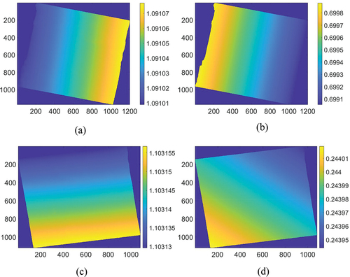
Table 4. Average of errors in error propagation maps using the law of variance propagation.

		SAR image #1	SAR image #2
Average of errors	Row ($i$)	1.1 Pixels	1.1 Pixels
	Column ($j$)	0.7 Pixels	0.2 Pixels
Time cost		2043.5 s	1844.2 s

A Monte Carlo simulation was used to verify the results of the error propagation maps (Zhen et al. 2022). During the simulation, random errors were set to be randomly generated by considering the correlations between them. The number of samples was set to 10,000 (Muthén and Muthén 2002), and the simulation results are summarized in Table 5. There was no difference between the propagated error values in Tables 4 and 5. However, the time cost when calculating the error budgets using the law of variance propagation was much smaller than that when using the Monte Carlo simulation. Regardless, error propagation maps were correctly generated. This result confirms that it is more efficient to calculate propagated errors using the law of variance propagation approach than using Monte Carlo simulation.

Table 5. Average of errors calculated using Monte Carlo simulation.

		SAR image #1	SAR image #2
Average of errors	Row ($i$)	1.1 Pixels	1.1 Pixels
	Column ($j$)	0.7 Pixels	0.2 Pixels
Time cost		346,136.6 s	298,642.6 s

The error propagation results were used to calculate the average propagated errors of SAR geocoding in pixel units. Because there is little difference between the maximum and minimum values of the propagated errors in each error propagation map, the average of the propagated errors can be set as the error budget. The random error follows a normal distribution with an expectation of zero, and the value of the error is the standard deviation. Therefore, the error budget can be set according to the confidence level listed in Table 6.

Table 6. Error budget set for each confidence level.

Confidence level		SAR image #1	SAR image #2
68.27%	Row ($i$)	1.1 Pixels	1.1 Pixels
	Column ($j$)	0.7 Pixels	0.2 Pixels
95.47%	Row ($i$)	2.2 Pixels	2.2 Pixels
	Column ($j$)	1.4 Pixels	0.5 Pixels
99.73%	Row ($i$)	3.3 Pixels	3.3 Pixels
	Column ($j$)	2.1 Pixels	0.7 Pixels

Root mean square errors (RMSEs) were calculated using the ICPs of each SAR image to verify the quality of the geocoding accuracy of the SAR images. RMSEs in the row (azimuth) and column (range) directions of ICPs in pixel units were calculated using SAR satellite imaging geometry based on range-Doppler equations. Table 7 lists the RMSEs of SAR images #1 and #2 before the geometric correction.

Table 7. RMSEs of the ICPs before geometric correction.

	SAR image #1	SAR image #2
Row ($i$)	4.4 Pixels	2.3 Pixels
Column ($j$)	5.8 Pixels	2.5 Pixels

The KOMPSAT-5 SAR images utilized in the experiments were Level 1A products with internal calibration of the RAW data by the vendor. SAR image #2 lies within an error budget of a 99.73% confidence level in the row direction. However, the geocoding accuracy of SAR images #1 and #2, except for the row direction of SAR image #2, exceeded the error budgets of all confidence levels, despite the vendor’s internal calibration. Therefore, an additional procedure to improve the geocoding accuracy is required. Geocoding accuracy can be improved by applying a GCP-based geometric correction model.

4.3 Second step: geometric correction

4.3.1 Removing multicollinearity

Section 4.1 presented the geometric correction model with eight error parameters. However, when analyzing the correlations among the eight error parameters, the correlations were very high for both SAR images. This indicates that multicollinearity exists in the model, which can be removed using feature selection. Feature selection is the process of reducing the number of parameters when developing a model, and can be performed by analyzing the variance inflation factors (VIFs) and correlation coefficients (Hair 2009; Mudereri et al. 2020). Finally, feature selection was verified by checking the increase in the RMSEs of the ICPs before and after feature selection using the GMM. If the feature selection is incorrect, the RMSEs will increase significantly, and if the feature selection is correct, the RMSEs will hardly change.

The VIFs are diagonal elements of the inverse of the correlation matrix (Belsley, Kuh, and Welsch 2005). Generally, multicollinear parameters have VIF values greater than 10 (Aggarwal and Kosian 2011). Table 8 lists the VIFs for the eight error parameters. However, feature selection using VIFs is not straightforward because all VIF values are high. In this case, a correlation coefficient analysis is performed instead of a VIFs analysis.

Table 8. VIFs of the eight error parameters. Because the VIFs of all parameters are high, feature selection can not be performed with VIFs analysis.

	$p_{sp,R_T\left(X\right)}$	$p_{sp,R_T\left(Y\right)}$	$p_{sp,R_T\left(Z\right)}$	$p_{sv(X)}$	$p_{sv(Y)}$	$p_{sv(Z)}$	$p_t$	$p_{ED,R}$
SAR Image #1	1.34 × 10^11	2.49 × 10^10	5.79 × 10^10	5.71 × 10^9	1.33 × 10^10	3.40 × 10^10	4.46 × 10^9	3.91 × 10^11
SAR Image #2	4.63 × 10^11	5.45 × 10^12	8.40 × 10^11	4.32 × 10^11	2.48 × 10^12	8.56 × 10^11	4.12 × 10^9	4.15 × 10^12

In Figure 4, the correlation coefficients between $p_{sp,R_T\left(X\right)}$, $p_{sp,R_T\left(Y\right)}$, $p_{sp,R_T\left(Z\right)}$, and $p_{ED,R}$ are almost 1 for both SAR images. Accordingly, only one of these parameters must be selected, which is determined as follows. The atmospheric and electronic delay error parameter ($p_{ED,R}$) directly affects the value of the slant range in the range equation, and the value of the slant range is determined by the satellite position and ground target position. Therefore, the atmospheric and electronic delay error parameter ($p_{ED,R}$) is expected to sufficiently reflect the satellite position and earth movement error parameters ($p_{sp,R_T\left(X\right)}$, $p_{sp,R_T\left(Y\right)}$, $p_{sp,R_T\left(Z\right)}$). After the removal of the satellite position and earth movement error parameters ($p_{sp,R_T\left(X\right)}$, $p_{sp,R_T\left(Y\right)}$, $p_{sp,R_T\left(Z\right)}$), there was almost no change in the RMSEs of the ICPs (Table 9). This result verifies that feature selection was performed correctly. After the feature selection, equations for the remaining five error parameters can be obtained, as shown in Equation (22)(22) $\begin{array}{cc}\hspace{0.17em}& i=f_{i\mathrm{\_}e\mathrm{\_}pa5}\left(X_T,Y_T,Z_T,p_{sv\left(X\right)},p_{sv\left(Y\right)},p_{sv\left(Z\right)},p_t,p_{ED,R}\right)\\ \hspace{0.17em}& j=f_{j\mathrm{\_}e\mathrm{\_}pa5}\left(X_T,Y_T,Z_T,p_{sv\left(X\right)},p_{sv\left(Y\right)},p_{sv\left(Z\right)},p_t,p_{ED,R}\right)\end{array}$(22) . A geometric correction model with five error parameters can be provided by applying the nonlinear case of GMM to Equation (22)(22) $\begin{array}{cc}\hspace{0.17em}& i=f_{i\mathrm{\_}e\mathrm{\_}pa5}\left(X_T,Y_T,Z_T,p_{sv\left(X\right)},p_{sv\left(Y\right)},p_{sv\left(Z\right)},p_t,p_{ED,R}\right)\\ \hspace{0.17em}& j=f_{j\mathrm{\_}e\mathrm{\_}pa5}\left(X_T,Y_T,Z_T,p_{sv\left(X\right)},p_{sv\left(Y\right)},p_{sv\left(Z\right)},p_t,p_{ED,R}\right)\end{array}$(22) .

(22) $\begin{array}{cc}\hspace{0.17em}& i=f_{i\mathrm{\_}e\mathrm{\_}pa5}\left(X_T,Y_T,Z_T,p_{sv\left(X\right)},p_{sv\left(Y\right)},p_{sv\left(Z\right)},p_t,p_{ED,R}\right)\\ \hspace{0.17em}& j=f_{j\mathrm{\_}e\mathrm{\_}pa5}\left(X_T,Y_T,Z_T,p_{sv\left(X\right)},p_{sv\left(Y\right)},p_{sv\left(Z\right)},p_t,p_{ED,R}\right)\end{array}$(22)

Table 9. Amount of RMSEs increase of ICPs after feature selection. Feature selection was performed correctly because the increases in RMSEs were very small or absent.

		8 parameters → 5 parameters	5 parameters → 2 parameters
SAR Image #1	Row ($i$)	0.0 Pixel (0.4 → 0.4)	0.0 Pixel (0.4 → 0.4)
	Column ($j$)	0.0 Pixel (0.6 → 0.6)	0.0 Pixel (0.6 → 0.6)
SAR Image #2	Row ($i$)	0.0 Pixel (0.4 → 0.4)	0.0 Pixel (0.4 → 0.4)
	Column ($j$)	− 0.1 Pixel (0.7 → 0.6)	0.0 Pixel (0.6 → 0.6)

A further step for multicollinearity analysis of the geometric correction model with the five error parameters was performed. Figure 6 and Table 10 present the correlation coefficients and VIFs of the five error parameters, respectively. It is confirmed by analyzing the values of VIF that $p_{sv\left(X\right)}$, $p_{sv\left(Y\right)}$, $p_{sv\left(Z\right)}$, and $p_t$ cause multicollinearity and are significantly correlated. Based on this result, only one of these parameters must be selected. The process of determining proceeds as follows. Time directly affects the satellite velocity in satellite orbit models. Therefore, the clock drift error parameter ($p_t$) is expected to sufficiently reflect the satellite velocity error parameters ($p_{sv\left(X\right)}$, $p_{sv\left(Y\right)}$, $p_{sv\left(Z\right)}$). After removing the satellite velocity error parameters ($p_{sv\left(X\right)}$, $p_{sv\left(Y\right)}$, $p_{sv\left(Z\right)}$), there was no change in the RMSEs of the ICPs (Table 9). Therefore, it can be concluded that the feature selection was performed correctly. Finally, equations for two error parameters can be obtained as shown in Equation (23)(23) $\begin{array}{cc}\hspace{0.17em}& i=f_{i\mathrm{\_}e\mathrm{\_}p2}\left(X_T,Y_T,Z_T,p_t,p_{ED,R}\right)\\ \hspace{0.17em}& j=f_{j\mathrm{\_}e\mathrm{\_}p2}\left(X_T,Y_T,Z_T,p_t,p_{ED,R}\right)\end{array}$(23) , and a geometric correction model with two error parameters can be provided by applying the nonlinear case of GMM. Figure 7 and Table 11 present the results of the analysis of the correlation coefficients and VIFs for the two error parameters. The correlation coefficient between the two error parameters was calculated as 0, and the VIFs were 1, confirming that there was no multicollinearity.

Figure 6. Correlation coefficients of the five error parameters. Except for $p_{ED,R}$, the correlations between the other parameters were calculated to be very high. Multicollinearity should be still removed: (a) SAR image #1 and (b) SAR image #2.

(23) $\begin{array}{cc}\hspace{0.17em}& i=f_{i\mathrm{\_}e\mathrm{\_}p2}\left(X_T,Y_T,Z_T,p_t,p_{ED,R}\right)\\ \hspace{0.17em}& j=f_{j\mathrm{\_}e\mathrm{\_}p2}\left(X_T,Y_T,Z_T,p_t,p_{ED,R}\right)\end{array}$(23)

Figure 7. Correlation coefficients of the two error parameters. There is no correlation between the two parameters: (a) SAR image #1 and (b) SAR image #2.

Table 10. VIFs of the five error parameters. Multicollinearity exists among $p_{sv\left(X\right),\hspace{0.17em}}\hspace{0.17em}{p}_{sv\left(Y\right),\hspace{0.17em}}\hspace{0.17em}{p}_{sv\left(Z\right),}{p}_t$.

	$p_{sv(X)}$	$p_{sv(Y)}$	$p_{sv(Z)}$	$p_t$	$p_{ED,R}$
SAR Image #1	6.38 × 10^8	3.64 × 10^8	3.90 × 10^8	4.08 × 10^9	1
SAR Image #2	4.17 × 10^8	5.95 × 10^9	4.71 × 10^8	6.14 × 10^9	1

Table 11. VIFs of the two error parameters. There is no multicollinearity between the two parameters.

	$p_t$	$p_{ED,R}$
SAR image #1	1	1
SAR image #2	1	1

4.3.2 Results of geometric correction

We named the geometric correction model with the two error parameters the non-multicollinearity (N-MC) model. Table 12 compares the RMSEs of the ICPs before and after geometric correction. The geometric correction results of the conventional orbit-based model and the N-MC model were almost identical when using 22 GCPs. As a result of geometric corrections with 22 GCPs using both models, the geocoding accuracy of the two SAR images was improved by approximately two to five pixels in the row and column directions. The results of the geometric correction with 22 GCPs using the N-MC model were analyzed as follows. The geocoding accuracy of SAR image #1 met error budgets of 68.27% confidence level in both row and column directions. The geocoding accuracy of SAR image #2 met an error budget of 68.27% confidence level in the row direction and an error budget of 99.73% confidence level in the column direction. After geometric correction, the geocoding accuracy of SAR image #2 in the column direction did not meet the 68.27% confidence level error budget. However, considering the errors in the GCPs, the result that the geocoding accuracy was improved within one pixel is reasonable. Figure 8 shows ortho-rectified SAR images generated by rectification with improved geocoding accuracy by applying the N-MC model.

Figure 8. Ortho-rectified SAR images with improved geocoding accuracy by applying the N-MC model overlaid on the aerial orthoimage: (a) SAR image #1 and (b) SAR image #2.

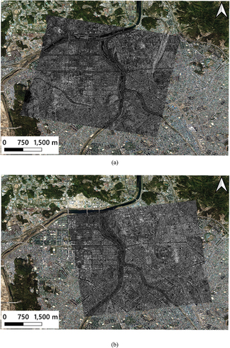
Table 12. RMSEs of ICPs before and after geometric correction. When 22 GCPs were used, the two models showed similar performance reaching subpixel accuracy.

			SAR image #1	SAR image #2
Before Geometric Correction		Row ($i$)	4.4 Pixels	2.3 Pixels
		Column ($j$)	5.8 Pixels	2.5 Pixels
After Geometric Correction using 22 GCPs	Orbit-based model (Conventional method)	Row ($i$)	0.5 Pixels	0.4 Pixels
		Column ($j$)	0.6 Pixels	0.6 Pixels
	N-MC model	Row ($i$)	0.4 Pixels	0.4 Pixels
		Column ($j$)	0.6 Pixels	0.6 Pixels
After Geometric Correction using 5 GCPs	Orbit-based model (Conventional method)	Row ($i$)	1.8 Pixels	1.3 Pixels
		Column ($j$)	1.3 Pixels	0.6 Pixels
After Geometric Correction using 1 GCP	N-MC model	Row ($i$)	0.4 Pixels	0.4 Pixels
		Column ($j$)	0.6 Pixels	0.6 Pixels

In GCP-based geometric correction, the theoretical minimum number of GCPs is determined by the number of parameters used in the geometric correction model. The orbit-based model, which is a conventional SAR geometric correction model, requires at least five GCPs because it uses nine orbital coefficients as parameters, whereas the N-MC model requires at least one GCP because it uses only two parameters. The obit-based model has high correlations between the parameters, indicating that multicollinearity exists among the parameters. Therefore, the values of the parameters estimated by applying GMM are unreliable. Multicollinearity does not exist in the N-MC model because no correlation exists between the two parameters. Therefore, the values of the parameters estimated using the N-MC model were reliable. Table 12 lists the results of geometric correction with the orbit-based model using five GCPs and 22 GCPs, and the results of geometric correction with the N-MC model using one GCP and 22 GCPs. The N-MC model showed the same results when using one GCP and 22 GCPs. However, the orbit-based model did not show the same results; geometric corrections using five GCPs were not as good as those using 22 GCPs. This is because some of the five GCPs had low accuracy even though only GCPs likely to be of relatively high accuracy were selected among the 22 GCPs. Nevertheless, the experiments demonstrated that the orbit-based model could perform geometric corrections with five GCPs, whereas the N-MC model could perform geometric corrections with only one GCP.

The quality of the GCPs is an important factor in GCP-based geometric correction. In general, accurate GCPs in SAR images can be obtained using corner reflectors. However, no such GCPs are available in the study area. All GCPs were manually picked. During manual collection of GCPs using artificial or natural objects, errors may occur in the GCPs. Therefore, we increased the redundancy by using a relatively large number of GCPs to compensate for the errors that may exist in the manually acquired GCPs. The experiments demonstrated that a relatively large number of GCPs evenly distributed in the SAR image can compensate for the errors in GCPs if there are insufficient high-quality and accurate GCPs. Further studies are required to obtain high-quality GCPs corresponding to the accuracy of corner reflectors to effectively perform GCP-based geometric corrections, even in the absence of GCPs acquired by corner reflectors.

5. Conclusions

In this study, we have proposed a framework to improve the geocoding accuracy by setting the error budget of the SAR image geocoding accuracy and applying a geometric correction model if the quality is lower than the predefined threshold. We first analyzed the correlations among the error sources affecting the geocoding accuracy of SAR images. This result made it possible to set the error budget accurately and develop the N-MC model, which is a geometric correction model without multicollinearity. The error budget was set by generating error propagation maps considering the correlation of the error sources. The error propagation map makes it easy for anyone to confirm the error budget at a glance throughout the SAR image. Furthermore, because the N-MC model uses only two parameters without multicollinearity, geometric correction can be performed with one accurate GCP, and the estimated values of the parameters are reliable. Our study shows that the geometric correction results of the conventional orbit-based model and the N-MC model are almost identical. Therefore, the N-MC model has a similar geometric correction performance to the conventional orbit-based model but has the advantage that it requires fewer GCPs and that the estimated values of the parameters are reliable.

Disclosure statement

No potential conflict of interest was reported by the author(s).

Data availability statement

The data are not publicly available because they are only accessible to Korean citizens owing to legal restrictions.

Additional information

Funding

This research was supported by a grant [20009742] of Ministry-Cooperation R&D program of Disaster-Safety, funded by Ministry of the Interior and Safety (MOIS, Korea; Ministry of the Interior and Safety).

References

- Ager, T. P., and P. C. Bresnahan. 2009. “Geometric Precision in Space Radar Imaging: Results from TerraSAR-X.” NGA CCAP Report.
- Aggarwal, V., and S. Kosian. 2011. “Feature Selection and Dimension Reduction Techniques in SAS.” EXL Service: New York, NY, USA.
- Alvarez, J., and B. Walls. 2016. “Constellations, Clusters, and Communication Technology: Expanding Small Satellite Access to Space.” In 2016 IEEE Aerospace Conference, Big Sky, MT, USA, 1–11. IEEE.
- Belsley, D. A., E. Kuh, and R. E. Welsch. 2005. Regression Diagnostics: Identifying Influential Data and Sources of Collinearity. New York: John Wiley & Sons.
- Breit, H., T. Fritz, U. Balss, M. Lachaise, A. Niedermeier, and M. Vonavka. 2009. “TerraSAR-X SAR Processing and Products.” IEEE Transactions on Geoscience and Remote Sensing 48 (2): 727–740. IEEE. doi:10.1109/TGRS.2009.2035497.
- Chen, P.-H., and I. J. Dowman. 2001. “A Weighted Least Squares Solution for Space Intersection of Spaceborne Stereo SAR Data.” IEEE Transactions on Geoscience and Remote Sensing 39 (2): 233–240. IEEE.
- Chen F., H. Xu, W. Zhou, W. Zheng, Y. Deng and I. Parcharidis. 2021.“ Three-dimensional deformation monitoring and simulations for the preventive conservation of architectural heritage: a case study of the Angkor Wat Temple, Cambodia.“ GIScience & Remote Sensing 58 (2): 217–234. Taylor & Francis. doi:10.1080/15481603.2020.1871188
- Choi, Y. J., S. H. Hong, and H. G. Sohn. 2019. “Geolocation Error Analysis of KOMPSAT-5 SAR Imagery Using Monte-Carlo Simulation Method.” Journal of the Korean Society of Surveying, Geodesy, Photogrammetry and Cartography 37 (2): 71–79. Korean Society of Surveying, Geodesy, Photogrammetry and Cartography.
- Covello, F., F. Battazza, A. Coletta, E. Lopinto, C. Fiorentino, L. Pietranera, G. Valentini, and S. Zoffoli. 2010. “COSMO-SkyMed an Existing Opportunity for Observing the Earth.” Journal of Geodynamics 49 (3–4): 171–180. Elsevier. doi:10.1016/j.jog.2010.01.001.
- Cumming, I. G., and F. H. Wong. 2005. “Digital Processing of Synthetic Aperture Radar Data.” Artech House 1 (3): 111–231. Boston.
- Curlander, J. C., and R. N. McDonough. 1991. Synthetic Aperture Radar. Vol. 11. New York: Wiley.
- Dunham, W. 1990. Journey through Genius: The Great Theorems of Mathematics. New York: Wiley.
- Eineder, M., H. Breit, N. Adam, J. Holzner, S. Suchandt, and B. Rabus. 2001. “Srtm X-SAR Calibration Results.” In IGARSS 2001. Scanning the Present and Resolving the Future. Proceedings. IEEE 2001 International Geoscience and Remote Sensing Symposium (Cat. No. 01CH37217), Sydney, Australia, 2: 748–750. IEEE.
- Eineder, M., C. Minet, P. Steigenberger, X. Cong, and T. Fritz. 2010. “Imaging Geodesy—Toward Centimeter-Level Ranging Accuracy with TerraSAR-X.” IEEE Transactions on Geoscience and Remote Sensing 49 (2): 661–671. IEEE. doi:10.1109/TGRS.2010.2060264.
- Frey, O., E. Meier, D. Nüesch, and A. Roth. 2004. “Geometric Error Budget Analysis for TerraSAR-X.” In Proceedings of the 5th European Conference on Synthetic Aperture Radar EUSAR, Ulm, Germany, 513–516.
- Ghilani, C. D. 2017. Adjustment Computations: Spatial Data Analysis. New Jersey: John Wiley & Sons.
- Hair, J. F. 2009. “Multivariate Data Analysis.”
- Han H., J. Kim, C. Hyun, S. H. Kim, J. Park, Y. Kwon, S. Lee, S. Lee and H. Kim. 2020. “Surface roughness signatures of summer arctic snow-covered sea ice in X-band dual-polarimetric SAR.“ GIScience & Remote Sensing 57 (5): 650–669. Taylor & Francis. doi:10.1080/15481603.2020.1767857
- Hong, S., Y. Choi, I. Park, and H.-G. Sohn. 2017. “Comparison of Orbit-Based and Time-Offset-Based Geometric Correction Models for SAR Satellite Imagery Based on Error Simulation.” Sensors 17 (1): 170. Multidisciplinary Digital Publishing Institute. doi:10.3390/s17010170.
- Hong, S. H., H. G. Sohn, S. P. Kim, and H. S. Jang. 2013. “Error Budget Analysis for Geolocation Accuracy of High Resolution SAR Satellite Imagery.” Journal of the Korean Society of Surveying, Geodesy, Photogrammetry and Cartography 31 (6_1): 447–454. Korean Society of Surveying, Geodesy, Photogrammetry and Cartography. doi:10.7848/ksgpc.2013.31.6-1.447.
- Hwang, Y., B. Lee, Y. Kim, K. Roh, O. Jung, and H. Kim. 2011. “GPS‐Based Orbit Determination for KOMPSAT‐5 Satellite.” ETRI Journal 33 (4): 487–496. Wiley Online Library. doi:10.4218/etrij.11.1610.0048.
- Ignatenko, V., P. Laurila, A. Radius, L. Lamentowski, O. Antropov, and D. Muff. 2020. “ICEYE Microsatellite SAR Constellation Status Update: Evaluation of First Commercial Imaging Modes.” In IGARSS 2020-2020 IEEE International Geoscience and Remote Sensing Symposium, Waikoloa, HI, USA, 3581–3584. IEEE.
- Jafarzadeh H., M. Mahdianpari, S. Homayouni, F. Mohammadimanesh and M. Dabboor. 2021. “Oil spill detection from Synthetic Aperture Radar Earth observations: a meta-analysis and comprehensive review.“ GIScience & Remote Sensing 58 (7): 1022–1051. Taylor & Francis. doi:10.1080/15481603.2021.1952542
- Jehle, M., D. Perler, D. Small, A. Schubert, and E. Meier. 2008. “Estimation of Atmospheric Path Delays in TerraSAR-X Data Using Models Vs. Measurements.” Sensors 8 (12): 8479–8491. Molecular Diversity Preservation International. doi:10.3390/s8128479.
- Jiao, N., F. Wang, H. You, J. Liu, and X. Qiu. 2020. “A Generic Framework for Improving the Geopositioning Accuracy of Multi-Source Optical and SAR Imagery.” ISPRS Journal of Photogrammetry and Remote Sensing 169: 377–388. Elsevier. doi:10.1016/j.isprsjprs.2020.09.017.
- Kim N., Y. Choi, J. Bae and H. Sohn. 2020. “Estimation and improvement in the geolocation accuracy of rational polynomial coefficients with minimum GCPs using KOMPSAT-3A.“ GIScience & Remote Sensing 57 (6): 719–734. Taylor & Francis. doi:10.1080/15481603.2020.1791499
- Koch, K.-R. 1999. Parameter Estimation and Hypothesis Testing in Linear Models. Berlin: Springer Science & Business Media.
- Lee, S.-R. 2010. “Overview of KOMPSAT-5 Program, Mission, and System.” In 2010 IEEE International Geoscience and Remote Sensing Symposium, Honolulu, HI, USA, 797–800. IEEE.
- Liang, W., Y. Wu, M. Li, and Y. Cao. 2022. “Adaptive Multiple Kernel Fusion Model Using Spatial-Statistical Information for High Resolution SAR Image Classification.” Neurocomputing 492: 382–395. Elsevier. doi:10.1016/j.neucom.2022.03.062.
- Loew, A., and W. Mauser. 2007. “Generation of Geometrically and Radiometrically Terrain Corrected SAR Image Products.” Remote Sensing of Environment 106 (3): 337–349. Elsevier. doi:10.1016/j.rse.2006.09.002.
- Montenbruck, O., E. Gill, and F. Lutze. 2002. “Satellite Orbits: Models, Methods, and Applications.” Applied Mechanics Reviews 55 (2): B27–28. doi:10.1115/1.1451162.
- Mudereri B. T., E. M. Abdel-Rahman, T. Dube, T. Landmann, Z. Khan, E. Kimathi, R. Owino and S. Niassy. 2020. “Multi-source spatial data-based invasion risk modeling of Striga (Striga asiatica) in Zimbabwe.“ GIScience & Remote Sensing 57 (4): 553–571. Taylor & Francis. doi:10.1080/15481603.2020.1744250
- Muthén, L. K., and B. O. Muthén. 2002. “How to Use a Monte Carlo Study to Decide on Sample Size and Determine Power.” Structural Equation Modeling 9 (4): 599–620. Taylor & Francis. doi:10.1207/S15328007SEM0904_8.
- Naftaly, U., and R. Levy-Nathansohn. 2008. “Overview of the TECSAR Satellite Hardware and Mosaic Mode.” IEEE Geoscience and Remote Sensing Letters 5 (3): 423–426. IEEE. doi:10.1109/LGRS.2008.915926.
- Oliver, C., and S. Quegan. 2004. Understanding Synthetic Aperture Radar Images. Chennai, India: SciTech Publishing.
- Qin, Y., D. Perissin, and L. Lei. 2013. “The Design and Experiments on Corner Reflectors for Urban Ground Deformation Monitoring in Hong Kong.” International Journal of Antennas and Propagation 2013: 1–8. Hindawi. doi:10.1155/2013/191685.
- Schubert, A., M. Jehle, D. Small, and E. Meier. 2009. “Influence of Atmospheric Path Delay on the Absolute Geolocation Accuracy of TerraSAR-X High-Resolution Products.” IEEE Transactions on Geoscience and Remote Sensing 48 (2): 751–758. IEEE. doi:10.1109/TGRS.2009.2036252.
- Schubert, A., M. Jehle, D. Small, and E. Meier. 2012. “Mitigation of Atmospheric Perturbations and Solid Earth Movements in a TerraSAR-X Time-Series.” Journal of Geodesy 86 (4): 257–270. Springer. doi:10.1007/s00190-011-0515-6.
- Schubert, A., D. Small, M. Jehle, and E. Meier. 2012. “COSMO-Skymed, TerraSAR-X, and RADARSAT-2 Geolocation Accuracy after Compensation for Earth-System Effects.” In International Geoscience and Remote Sensing Symposium (IGARSS), Munich, Germany, 3301–3304. IEEE. doi:10.1109/IGARSS.2012.6350598.
- Shafizadeh-Moghadam H., Q. Weng, H. Liu and R. Valavi. 2020. “Modeling the spatial variation of urban land surface temperature in relation to environmental and anthropogenic factors: a case study of Tehran, Iran.“ GIScience & Remote Sensing 57 (4): 483–496. Taylor & Francis. doi:10.1080/15481603.2020.1736857
- Shimada, M. 2018. Imaging from Spaceborne and Airborne SARs, Calibration, and Applications. Boca Raton, FL, USA: CRC press.
- Soumekh, M. 1999. Synthetic Aperture Radar Signal Processing. Vol. 7. New York: Wiley.
- Spinetti C., M. Bisson, C. Tolomei, L. Colini, A. Galvani, M. Moro, M. Saroli and V. Sepe. 2019. “Landslide susceptibility mapping by remote sensing and geomorphological data: case studies on the Sorrentina Peninsula (Southern Italy).“ GIScience & Remote Sensing 56 (6): 940–965. Taylor & Francis. doi:10.1080/15481603.2019.1587891
- Taylor, J. 1997. Introduction to Error Analysis, the Study of Uncertainties in Physical Measurements. Sausalito, California: University Science Books.
- Toutin, T. 2004. “Geometric Processing of Remote Sensing Images: Models, Algorithms and Methods.” International Journal of Remote Sensing 25 (10): 1893–1924. Taylor & Francis. doi:10.1080/0143116031000101611.
- Wermuth, M., A. Hauschild, O. Montenbruck, and R. Kahle. 2012. “TerraSAR-X Precise Orbit Determination with Real-Time GPS Ephemerides.” Advances in Space Research 50 (5): 549–559. Elsevier. doi:10.1016/j.asr.2012.03.014.
- Werninghaus, R., and S. Buckreuss. 2009. “The TerraSAR-X Mission and System Design.” IEEE Transactions on Geoscience and Remote Sensing 48 (2): 606–614. IEEE. doi:10.1109/TGRS.2009.2031062.
- Yang, J., C. Liu, and Y. Wang. 2014. “Detection and Imaging of Ground Moving Targets with Real SAR Data.” IEEE Transactions on Geoscience and Remote Sensing 53 (2): 920–932. IEEE. doi:10.1109/TGRS.2014.2330456.
- Zhang, L., T. Balz, and M. Liao. 2012. “Satellite SAR Geocoding with Refined RPC Model.” ISPRS Journal of Photogrammetry and Remote Sensing 69: 37–49. Elsevier. doi:10.1016/j.isprsjprs.2012.02.004.
- Zhen Z., L. Yang, Y. Ma, Q. Wei, H II. Jin and Y. Zhao. 2022. “Upscaling aboveground biomass of larch (Larix olgensis Henry) plantations from field to satellite measurements: a comparison of individual tree-based and area-based approaches.“ GIScience & Remote Sensing 59 (1): 722–743. Taylor & Francis. doi:10.1080/15481603.2022.2055381