Satellite flood detection integrating hydrogeomorphic and spectral indices

ABSTRACT

Satellite remote sensing is a highly valuable data source useful in the monitoring of surface water dynamics and an essential tool in flood risk management although several factors can interfere with the detection of water features. This study explores an approach that integrates satellite optical images and DEM-based hydrogeomorphic features to enhance real‐time identification of river flooding. Spectral indices, namely MNDWI and the combination of NDWI/NDTI, were taken from Sentinel-2 images and used to detect flooded areas, while DEMs were used to identify areas more exposed to river flooding using the Geomorphic Flood Index. The integration/overlapping of these layers allowed us to refine the final map with a significant detection improvement compared to those based exclusively on the segmentation of a spectral index. The proposed integrated approach was tested in five areas of the Piave river (Northern Italy) where a flooding event caused by the Vaia storm took place in October 2018. Results have been evaluated against reference maps produced manually in five selected areas, demonstrating good capabilities of the proposed procedure (mean accuracy 0.90), significantly reducing false alarms (Matthews Correlation Coefficient improvements among 0.02–0.43 in 4 out of 5 areas). The key advantages of such a procedure are the rapid application and the free and easy availability of the data that, in turn, allow for the investigation of large areas in the aftermath of an event.

KEYWORDS:

• Flood mapping
• remote sensing
• sentinel-2
• geomorphic flood index
• digital elevation models (DEM)
• vaia storm

1. Introduction

Storms and floods represent the most common type of natural disaster worldwide and the most significant in terms of economic damage. Between 2000 and 2019, floods represented 44% of all recorded disasters (EM-DAT the most comprehensive global database on natural and technological disasters) affecting about 1.6 billion people and a global loss of 651 billion US$ (UN Office for Disaster Risk Reduction (UNDRR) and UN Office for Disaster Risk Reduction (UNDRR), and Centre for Research on the Epidemiology of Disasters (CRED) 2020), losses that are expected to continue to increase due to climate change, economic growth, and urbanization (Albertini et al. 2022). According to the JRC PESETA IV final report on climate change impacts and adaptation in the EU and UK (Feyen et al. 2020), more than 170,000 people are exposed to the effects of river flooding every year, this number could triple by 2100 without the adoption of further measures. Catastrophic worldwide flooding in 2021 (Western Europe (Else 2021), China, and India (Pandey et al. 2021)) is an indication of the severity of the situation.

Flood responses require preparation and communication and are usually organized under emergency conditions, where a clear picture of the event characteristics is essential to support an intervention plan. Unfortunately, the flood extent determined through collecting in situ data (for instance, point-based flood perimeter observations from citizens) can be inaccurate, impractical, time-consuming, and costly (Anusha and Bharathi 2020). Moreover, these data are usually limited in spatial coverage and acquisition frequency. Consequently, remote sensing (RS) data are invaluable, providing continuous/uninterrupted, up-to-date, and historical satellite data and synoptic views of large areas. The availability of multi-source (instruments operating at visible, thermal, and microwave wavelengths of the electromagnetic spectrum), multi-scale, and multi-resolution RS data is invaluable in the estimation of the extent of flooded areas (Goffi et al. 2020).

SAR (Synthetic Aperture Radar) data, for instance, is proving to be a reliable source of information thanks to its operational capability in any weather and light conditions (D’Addabbo et al. 2016; Shen et al. 2019; Riyanto et al. 2022; Scarpino et al. 2018). The two-satellite Sentinel-1 constellation, which has become the main SAR data source, is largely used for flood detection analysis (Wu et al. 2019; Helleis et al. 2022) as it offers a free 12-day cycle of data to all its global users (6 days, except higher latitudes, combining Sentinel-1A and Sentinel-1B orbits). In some cases, the revisit times of Sentinel 1 data and other satellite SAR platforms can be too long for effective flood detection as SAR methodologies are mainly based on change detection and at least two images close to the flood event are required.

Retrieving information from optical data is usually more straightforward (Schumann 2015) and its ability to detect flood patterns is widely recognized and often used in the validation of more complex techniques. In fact, the use of optical imagery for the validation of SAR water extraction has become common practice (e.g. D’Addabbo et al. 2016; Clement, Kilsby, and Moore 2018; Yang et al. 2021). The two-satellite Sentinel-2 constellation is one of the mainstream noncommercial optical sensors with a high revisit frequency (5 days at the equator and 2–3 days at mid-latitudes) from the combination of Sentinel-2A and Sentinel-2B orbits, which makes it suitable for flood mapping. However, the presence of dense clouds can limit the use of optical sensors, which are valuable only when images free of clouds in the areas of interest are available. Sentinel-2 imagery is currently inserted in data source portfolios organized to tackle emergencies. For instance, the Copernicus Emergency Management Service (CEMS; https://emergency.copernicus.eu/) uses optical and/or SAR data based on the availability to provide timely and accurate information for emergency response and disaster risk management. Unlike SAR data, optical data do not necessarily require change detection and one single image can be sufficient for flood identification. In addition, geometrical and spectral characteristics make Sentinel-2 data unique when compared to other active and antecedent multispectral optical – satellite missions that are openly and freely accessible to all users.

The drawbacks of optical observations can limit the accuracy of flood detection due to the lack of full surface information leading to misdetection of water (see, e.g., Donchyts et al. 2016). Some of them, such as the presence of clouds, snow, ice, and shadows, can be reduced by using elevation data, such as Digital Elevation Models (DEMs) (Huang et al. 2018). Elevation data have been used to help identify floods underneath vegetation, since it is usually hard to detect water hidden under forest canopies in optical images, especially in bottomland forests and hardwood swamps (Wang, Colby, and Mulcahy 2002; Lang and McCarty 2009). Elevation data can also be used to downscale satellite flood maps by distributing the flooded area of the original coarse pixels among finer-resolution pixels. In some studies (Li et al. 2013; Huang, Chen, and Wu 2014; Fluet-Chouinard et al. 2015), the spatial allocation of water subpixels was improved by ranking the elevation or identifying drainage pixels from DEMs, or by producing inundation probability maps to downscale the extent of floods from satellites. The goal of such studies was to achieve subpixel scale water mapping consistent with the terrain and therefore more reasonable than traditional subpixel mapping algorithms merely based on spatial contiguity. Finally, DEMs can help to discern flooding from wet areas or low-depth flooded areas, which are not critical, especially during an emergency (Mueller et al. 2016; Huang et al. 2017). This can be achieved by calculating terrain indices (e.g. Geomorphic Flood Index (Samela, Troy, and Manfreda 2017), Height Above Nearest Drainage (Rennó et al. 2008), and Multi-resolution Valley Bottom Flatness (Gallant and Dowling 2003) that have been proposed in the literature to identify areas with higher probability of flooding.

Several studies have explored the use of topographic information to support flood detection strategies using optical data. However, official recommendations regarding the best approach for the use of elevation data to detect water bodies are still lacking and some do not provide sufficient details on how elevation data are used to support water mapping; others specify the chosen topographic parameter without providing the criteria for use (e.g. the criterion for thresholding the topographic feature, see, e.g., Chen et al. 2013; Donchyts et al. 2016; Cian, Marconcini, and Ceccato 2018), making these procedures hard to reproduce even for comparison purposes.

Based on these premises, this study aims to explore a pioneering approach integrating spectral indices from optical images and the Geomorphic Flood Index (GFI) to retrieve a realistic picture of areas flooded by rivers. The GFI has been chosen for its reliability, since it was specifically formulated to identify flood susceptibility and emerged as the best performing index out of several other morphological descriptors tested in comparative analyses carried out in different regions all over the world, varying in terms of topography, climate, extent, and degree of anthropization (see e.g., Manfreda et al. 2015; Samela et al. 2016; Samela, Manfreda, and Troy 2017; Albano et al. 2020). Its performances have been validated in the continental USA and in Europe (Samela, Troy, and Manfreda 2017; Tavares da Costa et al. 2019). It also assures reproducibility and replicability, since it can be easily obtained from a DEM and is used to perform a supervised threshold binary classification. The most recent contributors on this topic have also identified the GFI as the most informative univariate morphometric index for floodplain delineation (e.g. Magnini et al. 2022).

In the first phase of our study, different spectral indices from Sentinel-2 images were investigated both in isolation and combined for successful integration with the GFI. The extraction of water surfaces from optical data is commonly performed by using single spectral indices (Acharya et al. 2016). However, intensive transport processes in rivers occur during the passage of a flood wave (De Sutter, Verhoeven, and Krein 2001) and the high sediment load/turbidity, as well as the possible concurrence of debris flows/mud flows, could limit the ability of water indices to identify flooded pixels. Hence, a combination of appropriately selected indices could lead to better results by fine tuning suited thresholds. The integration of hydrogeomorphic analyses and pattern classifications can finally refine the detection to achieve more robust mapping compared to traditional approaches based exclusively on the segmentation of single water spectral indices.

All the procedural steps (selection of satellite indices, thresholding, and integration) were developed and evaluated for the case study of the 2018 Piave River flooding caused by the Vaia storm, which significantly impacted the Northeast regions of Italy. This is the typical event for which our method is intended, as the impacted area is large, morphologically heterogeneous, and embedded in different landscapes. In such complex contexts, it is particularly crucial to estimate the extent of flooded areas as soon as possible to coordinate the first field interventions and to provide a first estimate of the damage. The basin complexity enables us to select various sub-basin scenes that can act as different test sites to validate the procedure and evaluate the detection performance in different environmental scenarios.

Our final goal is to propose a reliable flood detection method that can offer as its main advantages the use of free and easily available data and the speed of assessment, thus allowing for the investigation of large areas.

2. Case study and data set: flooding of the Piave river (Italy) in October, 2018

2.1. Case study

A prolonged rain event hit Northern Italy between October 27 and 30, 2018, with strong winds and intense thunderstorms. The Vaia cyclone (as named by the Berlin, Freia University, FUB and Meteo, France) passed over the Alps, uprooting trees and causing the rapid increase in the water levels of the Livenza, Piave, Tagliamento, and Adige rivers. All four rivers reached the highest warning level, many areas were flooded, and an extensive amount of mud and debris flow occurred. These violent storms battered Italy for days and caused 29 casualties across all affected regions.

Among the impacted areas, the Piave basin in Veneto, which was the Italian region that paid the highest costs, was affected by a complex combination of sparse flood events, landslides, mudflows, and debris flows, with an estimated damage of 1 billion, 769 million EUR. The high topographic complexity of the basin and the variety of the phenomena makes it a particularly interesting location to test our flood mapping strategy.

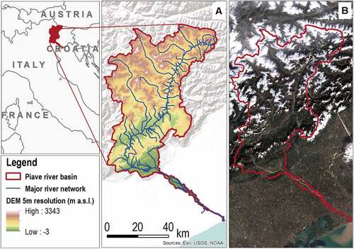
The Piave basin is located in the eastern Italian Alps, the river is 231 km long and flows into the Adriatic Sea, northeast of Venice. The watershed has a drainage basin of about 4100 km² and is characterized by a marked topography from high mountains to coastal areas below the sea level, with an average slope of 0.004 m m⁻¹. Figure 1 displays the geographical and topographical setting of the Piave basin. The river has been strongly influenced by several anthropogenic activities, such as the construction of dams, water diversions, gravel mining, and bank protections, as well as the occurrence of phases of deforestation and reforestation. As a result, the river has been exposed to considerable widening and incision phases (up to 2–3 m) (Ravazzolo et al. 2015). Comiti et al. (2011) reported a progressive shift from a dominant braided (multichannel) to a wandering morphology. However, more recently, this tendency appears to be changing, probably due to the abandonment of gravel mining. The climate is temperate-humid with an average annual precipitation of about 1350 mm. During the extreme weather event, the total rainfall reached about 715 mm in four days (data from Soffranco – Longarone, meteorological station, https://www.arpa.veneto.it/bollettini/storico/evento1/Mappa_PREC.htm (last accessed: 1/12/2021).

Figure 1. Geographical and topographical setting of the Piave river basin in Northern Italy. Panel A: 5-m resolution digital terrain model used for the study; Panel B: Satellite image acquired by Sentinel-2 on 31 October 2018 (after the extreme weather event).

2.2. Data set characteristics

The data set used for this case study:

• Digital Terrain Model (DTM) at 5 m resolution provided by the Veneto Region cartographic service (https://idt2.regione.veneto.it/idt/downloader/download, last accessed: 02/08/2022) (see Figure 1A). This product was released in 2007 and is based on elevation data (contours lines and elevations points) derived from the regional technical cartography (C.T.R.) at the 1:5,000 scale. The DTM is divided into tiles, distributed in ascii format, that correspond to those of the C.T.R (Terzariol 2014);

• Flood Hazard maps for three return periods with high, medium, and low probability of occurrence (T_R 30, 100 and 300 years) updated to 2019, kindly provided upon request by the Eastern Alps District Basin Authority. These maps were produced through a hydrologic analysis and a hydrodynamic modeling (mainly using 1D- hydraulic models) based on the measurements of the height of precipitation recorded on all the active rain-gauge stations existing in the area, historical time series of maximum annual values of precipitation, hydrometric levels recorded on gauged sections along the river, and related flow rates, where available (Distretto Idrografico delle Alpi Orientali 2016);

• Sentinel-2 optical images (tiles T32TQR and T32TQS) acquired on 31 October 2018 (after the storm passed) retrieved at no cost from the public European Space Agency’s (ESA) Scientific Data Hub (https://scihub.copernicus.eu/). All data acquired by the Multispectral Instrument (MSI) from the Sentinel-2 constellation were systematically processed up to Level 1C, a standard product of TOA (Top of Atmosphere) reflectance, composed of granules, also called tiles, of about 110 km × 110 km (10,980 × 10,980 pixels at 10 m of spatial resolution) ortho-images in UTM/WGS84 (Universal Transverse Mercator/World Geodetic System 1984) projection (Coluzzi et al. 2018). They are suitable for estimating spectral indices (Ko, Kim, and Nam 2015; Du et al. 2016) since the distributed data are radiometrically corrected.

The post-flood image is shown in Figure 1B.

3. Methods

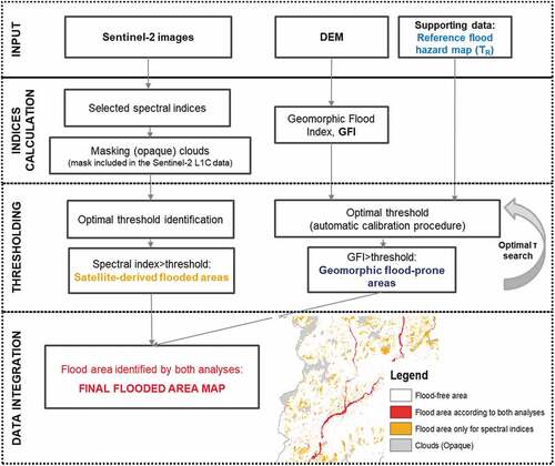
The methodology is based on a parsimonious integrated approach for the identification of areas flooded by rivers. The workflow of our analyses is shown in Figure 2, and the primary source of information is represented by Sentinel-2 optical data. The use of different water spectral indices is explored in this study by separately applying the general processing chain in Figure 2: the most appropriate thresholds to discriminate water areas are selected to produce flood/no-flood binary maps, which are combined with a hydrogeomorphic flood index (the GFI) able to discriminate the areas topographically susceptible to river flooding for a given return time, T_R (chosen according to the considered event). A performance analysis is then performed for each selected index (or combination of indices). This integration is aimed at producing a final flood map where false alarms (e.g. caused by shadows, clouds, snow, etc.) can be significantly reduced.

Figure 2. Workflow of the proposed integrated spectral/hydrogeomorphic approach to flood detection.

3.1. Detection of flooded areas using spectral indices from optical satellite images

The quantity of good-quality, high-frequency satellite products available to evaluate flooding effects has increased significantly over the last few years. The Sentinel series of satellites is a prime example of these remote data sources. Specifically, Sentinel‐2 is part of the European Space Agency Copernicus programme and consists of two twin satellites launched on 23 June 2015 and 7 March 2017. They provide freely available optical images for land services (e.g. imagery of vegetation, soil and water cover, inland waterways and coastal areas, and information for emergency services) with high spatial and temporal resolutions (Coluzzi et al. 2020; Ciancia et al. 2020; Greco et al. 2018). Free of clouds, Sentinel-2 images usually display the flooded areas very well (e.g. by an RGB composition) within the limits of the sensor resolution (see the UN-SPIDER recommended practice for flood mapping at https://www.un-spider.org/advisory-support/recommended-practices/recommended-practice-flood-mapping-and-damage-assessment).

We selected and processed the first available post-event Sentinel-2 Level 1C image with a low percentage of cloud cover. In order to include the whole Piave basin, two images (Section 2.2) were retrieved from ESA Copernicus Open Access Hub and mosaicked. Table 1 shows the Sentinel-2 bands used for this study:

Table 1. Main features of the Sentinel-2 bands adopted in this study.

Satellite name	Band information	Spectral resolution (center – $\mu m$)	Spatial resolution(m)
Sentinel-2	Band 3 (B3) – Green	0.560	10
	Band 4 (B4) – Red	0.665	10
	Band 8 (B8) – NIR	0.842	10
	Band 11 (B11) – SWIR	1.610	20
	Band 12 (B12) – SWIR	2.190	20

Methods used to detect water with multi- and hyperspectral (satellite) imagery are mainly based on the peculiar features of the spectral signature of water, which significantly absorbs more radiation at short-wave infrared (SWIR) than at Near Infrared (NIR) wavelengths. Several spectral indices have been formulated to identify water bodies by strengthening water-related information while, at the same time, reducing the non-water signal. In this study, we started from two of the most popular indices that are discussed significantly in the literature:

• the Normalized Difference Water Index (NDWI, Gao 1996; McFeeters 1996), representing the slope of the water spectral curve (Donchyts et al. 2016), defined as

(1) $NDWI={\frac{{\rho }_{GREEN}-{\rho }_{NIR}}{{\rho }_{GREEN}+{\rho }_{NIR}}}_{\hspace{0.17em}}$(1)

where ${\rho }_{GREEN}$ and ${\rho }_{NIR}$ are the reflectance of Green and NIR bands, respectively. The NDWI is the earliest water index, which has proven to be able to separate water from soil and vegetated surfaces but is less able to separate built-up areas whose spectral response results in relatively high NDWI values.

The Modified Normalized Difference Water Index (Xu 2006) is defined as

(2) $MNDWI={\frac{{\rho }_{GREEN}-{\rho }_{SWIR}}{{\rho }_{GREEN}+{\rho }_{SWIR}}}_{\hspace{0.17em}}$(2)

where ${\rho }_{GREEN}$ and ${\rho }_{SWIR}$ are the reflectance of Green and SWIR bands, respectively. This index can efficiently distinguish built areas and turbid water. The only disadvantage in this case is the coarser resolution (20 m) of the SWIR band that does not allow for the detection of water areas at full sensor resolution.

Considering that in the rising phase of the flood peak, especially after a rainstorm, water has a higher concentration of suspended particles, this specific extreme weather event also produced debris flow processes, and a significant increase in the turbidity of water was expected. As a result, the Normalized Difference Turbidity Index (NDTI; Lacaux et al. 2007) was also evaluated, possibly in combination with the previous indices, and is defined as follows:

(3) $NDTI={\frac{{\rho }_{RED}-{\rho }_{GREEN}}{{\rho }_{RED}+{\rho }_{GREEN}}}_{\hspace{0.17em}}$(3)

where ${\rho }_{RED}$ and ${\rho }_{GREEN}$ are the reflectance of green and NIR bands, respectively.

After computing the spectral indices, thresholds were imposed to segment and obtain the most reliable flood masks. Three strategies are reported in the literature (Wen et al. 2021): i) when ground reference data are available, local optimal thresholds can be determined (or trained) from the reference data; however, timely data in highly dynamic water landscapes (e.g. during flood events) are difficult to obtain. In this case, ii) predefined thresholds suggested by the original water indices inventors can be used, although these cannot guarantee satisfying results due to the complex water-land environments in the real world, or iii) locally adaptive thresholds, variable for different images, can be determined directly from the spectral index maps. All three ways of setting the threshold are suitable alternatives for the application of the proposed integrated approach.

For this specific case study, we decided to determine optimal local thresholds using the traditional manual method, as this can be a good solution to easily account for spatial information when the intensity contrast between different surface features is very low. A visual interpretation method was adopted, based on the comparison between the provisional maps obtained with different thresholds and the flood areas observed both with the Sentinel-2 natural color composite B4B3B2 and the false color composite B12B8B4 (Goffi et al. 2020). Once a suitable threshold is defined (best overlap), each final spectral map was segmented into a binary map, background was set to zero (all values below the threshold), and foreground was set to one (all values above the threshold).

All the processing steps were carried out using GIS tools and SNAP (Sentinel Application Platform).

3.2. Identification of locations geomorphologically prone to flooding

Identifying areas prone to potential flooding using hydrogeomorphic approaches is a consolidated procedure based on robust theories. The assumption is that fluvial morphology and floodplains are defined as distinguished landscape features historically shaped by the accumulated effects of floods (Manfreda, Di Leo, and Sole 2011; Nardi et al. 2019; Di Baldassarre et al. 2020). With the recent development of near-global coverage DEMs (e.g. SRTM, ASTER GDEM, and ALOS PALSAR), floodplains can be quickly identified for a variety of large scale environmental and socio-economic analyses (Marchesini et al. 2021). (Topography-based) hydrogeomorphic maps do not provide event-based flood extents and do not take into account flood dynamics, thus are not entirely comparable to flood hazard maps obtained from hydrologic/hydrodynamic analyses. Therefore, in accordance with the reference literature, hereinafter, they are referred to as flood-susceptibility maps or flood-prone areas map (see, e.g., Lindersson et al. 2021).

The flood-prone areas have been delineated in this study using a topographic descriptor (Geomorphic Flood Index (GFI)) (Samela, Troy, and Manfreda 2017) defined in Eq. 4(4) $GFI=ln\left(\frac{h_r}{H}\right)$(4) ,

(4) $GFI=ln\left(\frac{h_r}{H}\right)$(4)

In each basin location (each pixel), the GFI is computed by comparing two terms, both estimated from the DEM by tracing the flow directions downstream. The first terms consists of an empirically derived water level (h_r) calculated in each drainage network pixel using the following hydraulic scaling relation of bankfull depth $h_r=b{A}_r^n$ (Leopold and Maddock 1953; Nardi, Vivoni, and Grimaldi 2006; B. Dodov and Foufoula-Georgiou 2005; Dodov and Foufola-Georgiou 2006; Samela, Troy, and Manfreda 2017),

(5) $h_r=b{A}_r^n$(5)

where A_r is the contributing area in the cross river section, b is a scale factor, and n is a dimensionless exponent. b and n can be calibrated using paired values of $h_r$ and $\hspace{0.17em}{A}_r$ from streamflow observations (see, e.g., Nardi, Vivoni, and Grimaldi 2006; Samela, Troy, and Manfreda 2017) or estimated from the literature. In this study, the power law exponent n was assigned as the average among values found in the literature, equal to n = 0.3544, similar to what was described in Samela et al. (2018). The parameter b, instead, was assumed to be equal to one since it does not affect subsequent elaborations (as shown in Manfreda and Samela (2019)).

The second term of the GFI is the difference in elevation H (also named by Rennó et al. 2008 as Height Above Nearest Drainage, HAND) between each basin pixel and the nearest connected stream channel cell. From the computational point of view, the following steps are carried out: (i) in each river network pixel, the variable water depth $h_r$ is estimated; (ii) in each basin pixel, it is assumed that the potential source of flood hazard is represented by the closest river pixel, which is identified following the steepest hydrological paths; (iii) $h_r$ in the latter point is assigned to the basin pixel under examination; (iv) the difference in elevation H between these two points is computed; and (v) Eq (4)(4) $GFI=ln\left(\frac{h_r}{H}\right)$(4) is applied in the examined basin pixel to compute the GFI value.

The GFI can be used to identify flood-prone areas (hereafter named Geomorphic Flood Areas (GFA) by performing a supervised threshold binary classification calibrated using a reliable preexisting flood hazard map (a map that covers 2% of the basin of interest is sufficient, as shown by Samela, Troy, and Manfreda (2017)). The EU Floods Directive 2007/60/EC requires the basin authorities to provide flood hazard maps for three full scenarios with high, medium, and low probability of occurrence. Generally, these are detailed maps derived by a hydrologic/hydraulic modeling, yet incomplete at the basin level (often referred to the main river and major tributaries), and are costly to produce. They can serve as a training data set to identify the optimal discrimination threshold able to minimize the total misclassification error (sum of false-positive rate and false-negative rate calculated by comparison with the hydraulic flood hazard map). After the classifier has been trained, it is used to detect flood-prone areas over unstudied portions of the basin for the same return period (changing the return period of the hazard map used for calibration, the GFA changes accordingly). If no detailed hydraulic studies are available, Tavares da Costa et al. (2020) proposed a procedure that relaxes the dependence on hydraulic flood maps and instead uses geomorphic and climatic-hydrologic characteristics of the basin of interest.

In this processing chain, we suggest that the GFA map is determined in relation to the return period of the event. If no information relating to the estimation of the return time of the event is available, for the sake of safety, we suggest a precautionary approach to determining the GFA for the maximum return time available (typically 300–500-yr flood). Nonetheless, the use of a GFA map larger than necessary cannot introduce new false positives since it is used to confirm (or not) the flooded pixels already identified from the optical image. Pixels not identified as flooded by the optical image will never be considered flooded for the studied event, even if they are geomorphologically prone to flooding for a higher return time.

As regards our case study, Giovannini et al. (2021) investigated the main characteristics of the Vaia storm and reported that the 72 h accumulated precipitations had return periods higher than 200 years in most of the eastern Italian Alps. Among the official flood hazard maps available for calibration, we carefully determined the GFA map for the highest recurrence interval available (300-year return time), in order to capture as many areas that could be affected by a fluvial flooding. The resulting training area represented 14% of the Piave basin.

During the DTM terrain analysis, we noticed that the flat areas in the final portion of the basin produced a simulated river network that did not match the real network, shown on Google Earth and in Open Street Map. By analyzing some altimetric profiles on Google Earth, we also identified the presence of an embankment in the final meanders (with a width comparable with the cell size of our DTM and an elevation 4–5 m higher than the surrounding areas) that we believe to be artificial and built after the acquisition of the elevation data used to generate the DTM. These issues impacted hydro-topographic derivatives (e.g. flow directions, stream channels, and basin boundaries), and consequently, the embankment was introduced and two well-known pre-processing methods for treating flat areas/depressions in DTM were applied: i) a stream-burning algorithm in the final portion of the Piave river (3 m carving through the r.carve GRASS function (Mitasova et al. 1999) and using the river vector extracted from OpenStreetMap as auxiliary data; ii) a depression filling algorithm (based on the algorithm developed by (Jenson and Domingue 1988). As regards the flow direction determination, the eight-direction (D8) flow algorithm (O’Callaghan and Mark 1984) was used. These allowed for consistency with the correct stream network and hydrographic basin boundary.

GIS tools were used for data preparation and the calculation of hydrological parameters extracted from the DTM. The hydro-geomorphic analysis, the supervised linear binary classification, and performance measure evaluations were carried out using MATLAB.

3.3. Data integration

The final flood map was produced by overlapping the satellite and GFA maps, retaining only those pixels identified as flooded by both. This final integration of layers was carried out in a GIS environment. All data sets were georeferenced in the Roma 1940 Gauss Boaga Ovest projection system, resampled to the same 5 m pixel size. In fact, the spatial resolution of the DTM used for this study is higher than the resolution of the satellite images and a GFA map was also used to downscale the satellite flood map and the final product was provided at 5 m.

3.4. Performance evaluation

Emergency flood mapping and its performance evaluation cannot typically benefit from the support of extensive and timely independent information (orthophotos, field surveys, etc.). The performance of the procedure we aim to develop was evaluated by comparing our final flood maps with visual reference maps produced by manual mapping. Five frames (5 x 5 km each) were selected considering the areas of highest interest for flood emergency management purposes and placed along the course of the main river from north to south, leaving out high-mountain headwater catchments. Our five validation frames are representative of quite different contexts, enabling us to verify the versatility of the approach for detecting floods within challenging scenarios. The selected areas are highly heterogeneous both in terms of morphology and land cover composition, which are the main features that can limit detection success. They are also characterized by different soil texture within the first 50 cm of soil depth, a diverse lithology, and different types of soil permeability, as shown by some selected layers in Figures S5-S9 and Table S1 in supplementary materials.

Reference maps of the flooded areas were created from a direct visual inspection of the Sentinel-2 images using different band combinations and geomorphological criteria. Two experts contributed to the development of the reference maps and the performance evaluation. This process is largely time-consuming and requires operators with significant experience in remote sensing, geomorphology, and flood dynamics (Notti et al. 2018) and is difficult to carry out quickly and homogeneously in vast areas.

Both the produced flooded maps and the reference maps have a binary raster format (1-flooded, 0-not flooded). Each map was overlaid, and each pixel was labeled according to four possible entries: true positive (TP) for pixels correctly classified as flooded, true negative (TN) for pixels correctly classified as not flooded, false negative (FN) for undetected flooded areas, and false positive (FP) for flood-free areas erroneously classified as flooded. From the confusion matrix reporting the number of TP, FN, FP, and TN, several metrics for evaluating classification performances were determined, including some of the standard metrics most widely used and, in addition, two metrics considered more reliable for unbalanced class problems (specifically, F-score and Matthews Correlation Coefficient). In our case, the number of flood-free pixels in the reference map is much higher than the number of flooded pixels. The selected metrics are listed below:

True-positive rate (sensitivity, recall, and hit rate) defines how many correct predicted positive values occur among all positive samples of the benchmarking data set,

(6) $R_{TP}=\frac{TP}{\left(TP+FN\right)}$(6)

False-negative rate (Error Type II, underestimation) defines how many incorrect negative results occur among all positive samples of the benchmarking data set,

(7) $R_{FN}=\frac{FN}{\left(TP+FN\right)}=1-R_{TP}$(7)

True-negative rate (or Specificity) defines how many correct negative results occur among all negative samples of the benchmarking data set,

(8) $R{ }_{TN}=\frac{TN}{\left(TN+FP\right)}$(8)

False-positive rate (Error Type I, overestimation) defines how many incorrect positive results occur among all negative samples of the benchmarking data set,

(9) $R_{FP}=\frac{FP}{\left(TN+FP\right)}=1-R_{TN}$(9)

Accuracy defines the number of correct assessments among all the samples of the benchmarking data set,

(10) $ACC=\frac{\left(TN+TP\right)}{\left(TN+TP+FN+FP\right)}$(10)

Precision or positive predictive value (PPV) summarizes the fraction of samples assigned to the positive class that belongs to this class,

(11) $Precision=TP/\left(TP+FP\right)$(11)

F-score or the F-measure combines Precision and Recall (TPR) into a single score that seeks to balance both concerns. This is a popular metric for imbalanced classification and ranges between 0, if either the precision or the recall is zero, and 1.0, indicating perfect precision and recall,

(12) $F-score=\left(2\ast Precision\ast R_{TP}\right)/\left(Precision+TPR\right)$(12)

The Matthews Correlation Coefficient (MCC) is a measure of correlation between the binary classifications and is generally regarded as a more informative and true score if the class sizes vary (Chicco and Jurman 2020). The MCC produces a high score only if the prediction provides good results in all the four confusion matrix categories (true positives, false negatives, true negatives, and false positives), proportionally for both the size of positive elements and the size of negative elements in the data set.

(13) $MCC=\frac{TP\cdot TN-FP\cdot FN}{\sqrt{\left(TP+FP\right)\left(TP+FN\right)\left(TN+FP\right)\left(TN+FN\right)}}$(13)

MCC spans between −1 (total disagreement between prediction and benchmark model) and +1 (perfect match between prediction and benchmark model); a value of MCC equal to 0 suggests that results are no better than a random prediction.

4. Results

4.1. Detection of inundated areas using spectral indices from optical satellite images

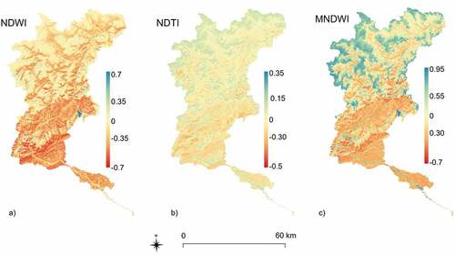
The water indices NDWI, NDTI, and MNDWI (Section 3.1) were calculated from the Sentinel-2 images, producing maps in Figure 3.

Figure 3. Results of the spectral water indices calculated from the Sentinel-2 images: a) Normalized Difference Water Index (NDWI); b) Normalized Difference Turbidity Index (NDTI); and c) Modified Normalized Difference Water Index (MNDWI).

The optimal thresholds were selected on the basis of on-screen visual comparisons between the binary maps with different thresholds and Sentinel-2 band combinations (the classical natural color composite B4B3B2 and the B12B8B4 color composite), as stated in Section 3.1.

Several threshold values within the range [−1;1] were evaluated starting from 0, which is the value commonly used to separate water from non-water pixels for spectral indices such as those selected in this study. In our fine-tuning process, the thresholds were repeatedly lowered or increased to obtain the best match and the best overlap between the binary maps and the flooded areas in the Sentinel-2 images.

The presence of sediments, shadows, and snow was the major problem in the thresholding of the NDWI (Figure 3a), whereas bare soil, buildings, and unshaded snow mixed with clouds were the main source of errors in the case of the NDTI (Figure 3b). To detect whole flooded areas, we opted for the integration of the NDTI and NDWI maps and an initial binary map was produced by combining the pixels flagged as flooded according to the NDTI map (NDTI>0) with those obtained for NDWI>0.30.

The main drawbacks of using the MNDWI index (Figure 3c) were the coarser resolution (20 m) and the presence of areas upstream covered by snow and shadows that show MNDWI values similar to those of water. Inefficient thresholding can imply the misclassification of cultivated areas in the southern part of the basin, which are confused with water areas or, on the contrary, can determine the presence of holes inside the major river. The final map was produced by selecting a threshold value (MNDWI>0) that significantly reduces both the number of pixels incorrectly labeled as water and the presence of artificial holes inside the major river.

The issue of cloudiness, which affects all the indices analyzed, could be reduced by integrating elevation data. In addition, the cloud mask provided with the Sentinel-2 image was applied to remove opaque clouds. The pixels within the polygons delimitating opaque clouds eventually detected as water were consequently neglected.

Both strategies here examined (NDTI/NDWI and MNDWI binary maps) seemed to be good candidates for the scope and were evaluated in the second phase for integration with geomorphological information.

Results of the segmentation of the NDWI, NDTI, and MNDWI maps using different threshold values are described in the supplementary material.

4.2. Identification of locations geomorphologically prone to flooding

The satellite maps in Section 4.1 are expected to be disturbed by a series of errors, which can be reduced by coupling a hydrogeomorphic analysis with the DTM.

Using the GFI map from the DTM and the hydraulic flood hazard map from the District Basin Authority, the binary classification introduced in Section 3.2 was performed and the flood susceptible areas were identified (Figure 4, on the right). Performances obtained during calibration are summarized in Table 2 and the Receiver Operating Characteristic (ROC) curve in Figure 4, on the left. The ROC curve illustrates the ability of a binary classifier system and is created by plotting the true-positive rate (RTP) against the false-positive rate (RFP) as the discrimination threshold is varied. Its area under the curve (AUC) provides an aggregate measure of performance across all possible classification thresholds and ranges in value from 0 to 1. The diagonal line from the bottom left to the top right corners, the line of no discrimination (red line In Figure 4a), represents a random classifier and has an AUC equal to 0.5. An AUC of 1 corresponds to a perfect classifier.

Figure 4. Receiver operating characteristics (ROC) curve obtained calibrating the geomorphic flood index (GFI) in the Piave river basin. the 300- years flood hazard map produced by the Eastern Alps district basin authority using hydraulic models was used for calibration. on the right, the resulting geomorphic flood-prone areas map.

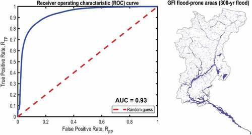
Table 2. Value of the optimal classification threshold and relative performance measures obtained by calibrating the threshold binary classification based on the GFI for the Piave river basin for the 300-year return period. The AUC value that aggregates the performance of the classifier at all threshold values is also reported.

Piave River Basin
DTM resolution (m)	GFI Optimal Threshold	True Positive Rate RTP	False Negative Rate RFN	True Negative Rate RTN	False Positive Rate RFP	Area Under the ROC curve AUC
5	−0.684	84%	16%	88%	12%	0.928

4.3. Data integration and performance evaluation

Finally, the (binary) flood maps from spectral indices (NDTI/NDWI and MNDWI) and the GFI map were overlaid. At this stage, a pixel-to-pixel comparison was performed, as explained in Section 3.3, confirming only the pixels identified by both the spectral and hydrogeomorphic indices as flooded.

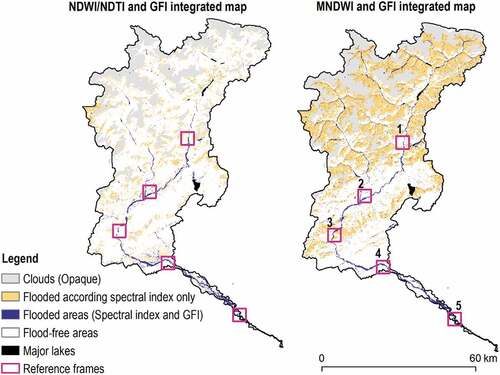
Figure 5 depicts the pixels flooded according to both analyses in dark blue, while the pixels flooded only according to the spectral indices are in Orange. These last will be neglected from now on. Flood-free areas (white) and opaque cloud coverage (gray) are also shown. Five reference frames (purple polygons in Figure 5) were selected in the high-risk areas and placed along the course of the main river, as described in Section 3.4

Figure 5. This image summarizes the results of the steps of the proposed approach: the dark blue pixels represent the areas identified both as flooded and flood-prone to river inundation by the spectral and hydrogeomorphic indices. these pixels were considered as the flooded area in the final map. the areas identified as flooded only according to the spectral indices are depicted in Orange and will be neglected. flood-free areas (white) and opaque cloud coverage (gray) provided along the Sentinel-2 image are also shown. Purple frames indicate the areas selected for the performance evaluation.

4.4. Performance evaluation results

Different contingency maps were obtained by comparing the reference flood maps with the NDTI/NDWI and MNDWI flood maps, pre- and post-integration with the GFI. They are shown in Figure 6 and 7, respectively, while Table 3 and Table 4 report the performance measures.

Figure 6. Contingency maps for 5 selected areas (each area is 5 × 5 km) by comparing the reference flood inundation maps (produced manually by experts through visual interpretation) and the flooded areas identified using NDTI and NDWI. In particular, the panels show the results before (1a to 5a) and after (1b to 5b) the correction with the GFI. Green, black and red colors indicate agreement, underestimation and overestimation, in this order.

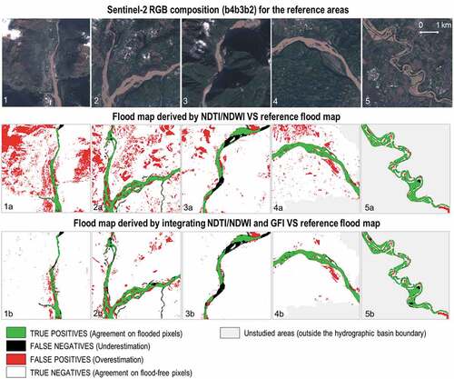
Figure 7. Contingency maps for 5 selected areas by comparing the reference flood inundation maps (produced manually by experts through visual interpretation) and the flooded areas identified using the MNDWI. in particular, the panels show the results before (1a to 5a) and after (1b to 5b) the correction with the GFI. Green, black and red colors indicate agreement, underestimation and overestimation, in this order.

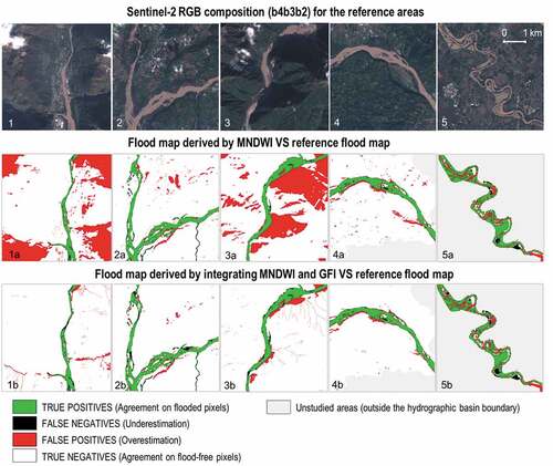
Table 3. Summary of performance measures calculated over 5 selected areas. Area 1a to area 5a report the results of the comparison between the reference map and the NDTI/NDWI flood map; area 1b to area 5 b report the results of the comparison between the reference map and the NDTI/NDWI flood map corrected with the integration with the GFI.

	RTP	RFN	RTN	RFP	ACC	Precision	F-score	MCC
Flood map derived by NDTI/NDWI VS reference flood map
Area 1a	0.89	0.11	0.78	0.22	0.79	0.12	0.21	0.28
Area 2a	0.91	0.09	0.83	0.17	0.83	0.35	0.51	0.50
Area 3a	0.61	0.39	0.94	0.06	0.92	0.42	0.50	0.46
Area 4a	0.97	0.03	0.92	0.08	0.92	0.51	0.67	0.67
Area 5a	0.93	0.07	0.76	0.24	0.86	0.84	0.88	0.70
Flood map derived by integrating NDTI/NDWI and GFI VS reference flood map
Area 1b	0.81	0.19	0.98	0.02	0.98	0.61	0.70	0.69
Area 2b	0.84	0.16	0.95	0.05	0.94	0.61	0.71	0.69
Area 3b	0.57	0.43	0.98	0.02	0.96	0.73	0.64	0.62
Area 4b	0.96	0.04	0.97	0.03	0.97	0.74	0.84	0.83
Area 5b	0.90	0.10	0.77	0.23	0.84	0.84	0.87	0.68

Table 4. Summary of performance measures calculated over 5 selected areas. Area 1a to area 5a report the results of the comparison between the reference map and the MNDWI flood map; area 1b to area 5 b report the results of the comparison between the reference map and the MNDWI flood map corrected with the integration of the GFI.

	RTP	RFN	RTN	RFP	ACC	Precision	F-score	MCC
Flood map derived by MNDWI VS reference flood map
Area 1a	0.89	0.11	0.74	0.26	0.74	0.10	0.18	0.25
Area 2a	0.89	0.11	0.97	0.03	0.96	0.73	0.80	0.78
Area 3a	0.95	0.05	0.72	0.28	0.74	0.20	0.32	0.36
Area 4a	0.96	0.04	0.96	0.04	0.96	0.67	0.79	0.78
Area 5a	0.92	0.08	0.44	0.56	0.72	0.69	0.79	0.42
Flood map derived by integrating MNDWI and GFI VS reference flood map
Area 1b	0.81	0.19	0.98	0.02	0.98	0.60	0.69	0.68
Area 2b	0.83	0.17	0.98	0.02	0.97	0.81	0.82	0.80
Area 3b	0.90	0.10	0.97	0.03	0.96	0.65	0.76	0.75
Area 4b	0.95	0.05	0.97	0.03	0.97	0.77	0.85	0.84
Area 5b	0.89	0.11	0.46	0.54	0.71	0.69	0.78	0.40

By comparing the panels in Figure 6 and Figure 7, we notice that the maps exclusively from the spectral indices (from 1a to 5a) are affected by significant errors, whereas a combined analysis using the hydrogeomorphic index (from 1b to 5b) largely reduces overestimation errors (red pixels) with a slight increase in underestimation errors (black pixels).

According to Table 3 and Table 4, the RFP decreases, while the RFN increases. In this regard, we recall that the flood-free pixels (total negative samples at the denominator of the RFP in Eq. 9)(9) $R_{FP}=\frac{FP}{\left(TN+FP\right)}=1-R_{TN}$(9) are significantly more than flooded pixels (total positives in the denominator of the RFN in Eq. 7(7) $R_{FN}=\frac{FN}{\left(TP+FN\right)}=1-R_{TP}$(7) ); hence, even a slight increase of the FN can produce a notable increase in the RFN, while a consistent reduction in FP still produces a small reduction in the RFP. The F-score and the MCC overcome this imbalanced data set issue and give us a clearer picture of the method performance. Both the metrics account for an improvement by combining spectral and hydrogeomorphic information. For example, frames 1, 2, and 3 of Figure 6 show that the spectral water indices incorrectly classify residual clouds as water (clouds such as cirrus have a signature similar to water, Coluzzi et al. 2018), while the integration with the GFI certainly reduces this error: before correction using the GFI, the undetected clouds in these scenes are classified as false positives (1a to 3a); after correction using the GFI, they are classified as true negatives (1b to 3b) (for instance, Area 1 for the NDTI/NDWI map goes from an MCC of 0.28 to 0.69; Area 1 for the MNDWI map goes from an MCC of 0.25 to 0.68). The accuracy ranges from 94% and 98% for both combinations, with the exclusion of frame 5, where the integration with the GFI does not improve the final F-score and MCC values.

The comparison of the performance measures for the flood map by integrating NDTI/NDWI and GFI and MNDWI and GFI (Table 3 and Table 4 from 1b to 5b) shows values fairly comparable for areas 1, 2, and 4. However, the values are significantly different for the remaining two frames. In frame 3, the final flood map from MNDWI and GFI shows a very low RFN value (0.10) and a very high RTP (0.90) compared to the 0.57 RTP value and the 0.43 RFN value of the flood map from using NDTI/NDWI and GFI. A detailed visual inspection reveals that the majority of the flooded areas that are underestimated by the integration of NDTI/NDWI and GFI are located under shadow zones. This result shows that the integration of MNDWI and GFI can better detect shaded flooded areas; this is probably due to its spectral characteristics (mainly the inclusion of the SWIR band). In the case of the frame 5, the integration of MNDWI and GFI produces a flood map with an RFP value of 0.54, higher than the RFP value of the NDTI/NDWI plus GFI flood map (0.23). The visual examination of the Sentinel-2 band combinations shows that the overestimated flooded areas of the integration of MNDWI and GFI flood map include parts of roads and sloped areas covered with dense vegetation located in proximity to the river.

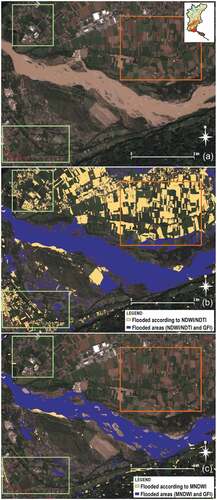
A paradigmatic example of the crucial role played by the GFI in the reliability of the flood detection is presented in Figure 8: the orange polygon in panel (b) shows misclassified rural fields largely eliminated after integration with the GFI; the green polygons (panel b) delimit urbanized areas with rooftops erroneously labeled as flooded by the NDTI/NDWI, which were removed after integration with the GFI. Panel (c) depicts the same study area, mapped by integrating MNDWI and GFI.

Figure 8. (a) RGB composition (R: Band 4, G: Band 3, B: Band 2) of a portion of the study area and (b) corresponding map produced by combining NDTI/NDWI with the GFI. Examples of areas misclassified as flooded are in the boxes: green for urban areas (mainly buildings), Orange for cultivated fields. We can distinguish rooftops and ground features detected as flooded by the spectral indices. Some of them were removed after the introduction of the GFI, while others that remained in the final map in accordance with the GFI, were also found to be overestimations. (c) same study areas mapped by integrating MNDWI and GFI.

5. Discussion

The drawbacks and potential of extracting inundated areas from optical sensors emerged using several spectral indices from Sentinel-2 images. These indices were combined with the Geomorphic Flood Index demonstrating the improvements by using an integrated spectral-hydrogeomorphic analysis.

The main detection limits to our approach were due to the complexity of the landscapes in the background of water, which makes it difficult to find one single optimal threshold on the basis of the trade-off between over and under estimation over the whole area: 1) the spectral indices NDTI/NDWI failed to detect water in many minor order streams, especially in the headwater catchments in the north of the basin, probably due to the inability of the turbidity index NDTI to detect clean water and the high threshold applied to the NDWI to avoid over detection in wet vegetated areas; 2) overestimation errors appear in the floodplains along the valley and approaching the outlet of the river, with several agricultural areas/fields that were erroneously indicated as flooded. The introduction of the GFI reduced this misclassification, thereby improving the detection performance significantly.

MNDWI performance showed that the segmented map (20 m) accurately depicted the whole river network, the permanent water bodies, and the flooded areas. When investigated at a more local scale, it was possible to distinguish the bars inside the river in the alluvial plain area, indicating a good level of detail in the discrimination between flooded and non-flooded pixels, also at a 20-m resolution. The main issues with the MNDWI-based flood map were due to hilly shadows, clouds, and cloud shadows, which were widespread in the upper part of the basin.

A quantitative measure of performance was made for five selected areas (purple frames shown in Figure 5) using reference maps produced for this scope. To summarize, we can make some general considerations:

1. The use of the GFI significantly reduced the errors that are intrinsic to the use of optical information, such as residual clouds, for both the two combinations of indices.

2. Looking at the performance measures in the five selected frames, which focus on areas along the river, the two combinations of indices provided comparable values and behaved as valid alternatives. Slight accuracy differences and error types were determined by the specific spectral information included in the indices.

3. The optimal binary map combining NDTI/NDWI performed well in detecting water along the main watercourse but failed in identifying water in minor order streams. The use of the NDTI, which was precious for discriminating turbid water, was not just as effective in discriminating clear water. The contextual difficulty in setting a threshold to the NDWI to separate water from wet vegetation and wet bare soil caused a worse result that, however, was confined to high-elevation areas not affected by the flood. The overall misclassification errors, although fewer compared to the MNDWI optimal binary map, could not always be removed with the introduction of the GFI.

4. The integration of MNDWI and GFI achieved better results especially in shaded areas likely because of the presence of the SWIR band in the MNDWI.

5. The MNDWI map had more benefits from integration with the GFI because the error types produced by this spectral index mainly involve overestimation that was ideal for removal by the GFI and efficiently to detect the minor order streams.

Among the advantages of this combined approach, we expect that the accuracy of the final flood map is less dependent on the choices of the spectral indices thresholds. Therefore, we expect that the performance of the integrated spectral/hydrogeomorphic approach is less sensitive to the uncertainty characterizing the use of spectral indices alone, in particular for threshold values causing excessive overprediction of flooded pixels. In our future studies on the development and improvement of flood detection strategies, we aim to further investigate this aspect, e.g. by performing sensitivity analyses of the thresholding.

We highlight that the GFI strongly depends on the quality of the DEM/DTM and the supporting data (flood hazard maps) used for calibration. In particular, DEM reliability is a crucial point in detection success: using high-resolution, high-accuracy (e.g. LiDAR DEM) and, hopefully, up-to-date DEMs are essential to reduce possible misclassifications. In fact, the acquisition time of the topographic data used to generate the DEM can be different from the acquisition time of satellite images. In that time window, land use and land cover changes can develop modified landscape and terrain elevations, altering the flow directions. The position of the river’s main watercourse can also change over time and, while satellite images can see the active channel pathways, DEM-derived flow paths can no longer be coherent to current paths. Relying on incorrect DEM-derived flow paths may result in the erroneous exclusion of some flooded areas. Unfortunately, it is common that local elevation minima (pits or closed depressions) and flat areas exist in a grid DEM and that hydro-topographic derivatives (e.g. flow directions and accumulations, stream channels, and basin boundaries) are impacted by this issue. Therefore, pre-processing conditioning procedures, are traditionally applied to deal with it. We are aware that this might unrealistically change DEM elevations, introduce differences in the calculation of the H (HAND) required for the GFI equation, and change subsequent depth estimates in later analyses. However, hydrologic conditioning might be necessary to obtain consistency with the real stream network, which is essential, and we believe that this does not affect the overall result of our analysis. We recall, in fact, that the proposed procedure aims to derive the extent of the flooded area, not the inundation depths, and that the water depths h_r used to derive the GFI are approximate estimates not used to identify flood-prone pixels (a supervised linear binary classification identifies them). The estimates of h_r values could be improved by calibrating the hydraulic scaling relationship of Eq. 5(5) $h_r=b{A}_r^n$(5) over the specific basin. However, it must be taken into account that calibrating the scaling law requires additional data collection and computational effort and there is the possibility that the gain obtained in terms of better estimates of h_r is reduced and not paid off due to several other sources of uncertainty associated with i) the H calculation, which depends on the terrain model quality, accuracy, and resolution; ii) the calibration of the threshold, which depends on the standard flood hazard map used to train the binary classification (its quality, its extent over the basin); iii) all the potential error sources related to the optical image characteristics and their processing.

It is important to underline that we aim to propose a flood mapping procedure that can be generalized, reproduced and replicated in any context. For this reason, we intentionally did not include in the proposed workflow other kinds of information typically available only in data-rich environments (e.g. continuous and real-time data from gauging stations or other in-situ data), although they are extremely useful for describing post-event scenarios. It is implied that in case of availability of valuable information/additional analysis for an occurred flood event, they can always complement the flood detection method here presented.

Surface complexity and atmospheric conditions are the main source of uncertainty related to the use of Sentinel-2 images. Improvements can be achieved through i) the use of additional higher resolution optical images; ii) the introduction of methods specifically proposed for removing clouds (Hagolle et al. 2010; Qiu, Zhu, and He 2019; Zhu, Wang, and Woodcock 2015) and shadows (Magno et al. 2021; Li, Sun, and Yu 2013; Sheng, Su, and Xiao 1998) in Sentinel-2 data; iii) attempting to solve problems related to the choice of a single threshold of the spectral indices, e.g. by establishing local variable thresholds that could be determined automatically (Otsu 1979; Donchyts et al. 2016). All these solutions can be introduced in the proposed integrated approach without distorting its logic and benefits.

6. Conclusion

The extraction of water surfaces from optical data is rather straightforward in theory; however, in practice, it is extremely challenging to develop standard procedures suited to complex areas. Applications for flood detection require specific strategies; in fact, the spectral response of flooded areas may be much more complex than the clear water response. Other surface features, particularly in the wet vegetated zones that are typically present in post-flood images, can be easily mistaken for floods leading both to false-positive and false-negative detection.

We have discussed the application of an integrated approach to detect flooded areas using Sentinel-2 optical images and a DTM. Spectral indices (i.e. NDWI and NDTI together; MNDWI alone) were calculated and segmented to distinguish flooded and flood-free pixels, and the resulting maps were combined with a flood susceptibility map from the GFI hydrogeomorphic index to improve classification.

The results of the application of our method on the Piave event revealed that there are significant possibilities with some limits for spectral indices and with their integration with the GFI. Results show good identification capabilities of areas affected by flooding, proving the ability of an integrated approach in improving results by largely reducing the false alarms due to shadows, cloud contamination, and wet vegetation, which can deceive the spectral indices (False-Positive Rates decreased in all cases, and Matthews Correlation Coefficients improved between 0.02 and 0.43 in 4 out of 5 areas).

The hydrogeomorphic analysis depends on the site structure and is independent of the specific flood event. Therefore, GFI susceptibility maps can be produced in advance by emergency management agencies, ready in the case of extreme weather events. The full procedure could also be repeated over time to provide an insight into the flood extent change over specific periods, providing valuable information on flood dynamics. For the replication of the procedure in cases with similar complexity levels (large-scale analysis with the presence of heterogenous landscapes and different morphological areas), improved performance is expected from the combination of MNDWI and the GFI.

The key advantage of the proposed procedure is its speedy implementation, across large and complex geographical areas and the ready availability of free data on a global scale, such as remotely sensed images and remotely sensed DEMs (e.g. SRTM DEM). Data that could be used to provide a timely and accurate representation of post-flood conditions in order to support flood-response efforts and damage assessment inform mitigation decision-making and advise the general public.

Author contributions

Caterina Samela and Rosa Coluzzi contributed to conceptualization and methodology; Rosa Coluzzi contributed to analysis of satellite data; Caterina Samela contributed to hydrogeomorphic analysis, data integration, and performance evaluation; Caterina Samela, Rosa Coluzzi, and Maria Lanfredi contributed to writing—original draft preparation; Caterina Samela, Rosa Coluzzi, Vito Imbrenda, Salvatore Manfreda, and Maria Lanfredi contributed to writing—review and editing; Maria Lanfredi contributed to funding acquisition. All authors have read and agreed the published version of the manuscript.

Acknowledgements

We would like to thank Paula Preston, Grad. CIPD, for proofreading the English in this paper.

Disclosure statement

The authors declare that they have no known competing financial interests or personal relationships that could have appeared to influence the work reported in this paper.

Data availability statement

The authors confirm that the data supporting the findings of this study is available within the article and its supplementary materials. The datasets generated during this study are available in the following link: https://drive.google.com/drive/ folders/1pyD_3pDilaUb-DuawCubhiHlb526UZyj?usp=sharing. Anyway,they are available on request from the corresponding author.

Supplementary material

Supplemental data for this article can be accessed online at https://doi.org/10.1080/15481603.2022.2143670

Additional information

Funding

This work was supported by the MIUR (Italian Ministry of Education, University and Research), OT4CLIMA PON project.

References

- Acharya, T. D., D.H. Lee, I.T. Yang, and J.K. Lee. 2016. “Identification of Water Bodies in a Landsat 8 OLI Image Using a J48 Decision Tree.” Sensors 16 (7): 1075. doi:10.3390/s16071075.
- Albano, R., C. Samela, I. Crăciun, S. Manfreda, J. Adamowski, A. Sole, Å. Sivertun, and A. Ozunu. 2020. “Large Scale Flood Risk Mapping in Data Scarce Environments: An Application for Romania.” Water 12 (6): 1834. doi:10.3390/w12061834.
- Albertini, C., D. Miglino, V. Iacobellis, F. De Paola, and S. Manfreda. 2022. “Delineation of Flood-Prone Areas in Cliffed Coastal Regions through a Procedure Based on the Geomorphic Flood Index.” Journal of Flood Risk Management 15 (1): e12766. doi:10.1111/jfr3.12766.
- Anusha, N., and B. Bharathi. 2020. “Flood Detection and Flood Mapping Using Multi-Temporal Synthetic Aperture Radar and Optical Data.” The Egyptian Journal of Remote Sensing and Space Science 23 (2): 207–219. doi:10.1016/j.ejrs.2019.01.001.
- Chen, Y., C. Huang, C. Ticehurst, L. Merrin, and P. Thew. 2013. “An Evaluation of MODIS Daily and 8-Day Composite Products for Floodplain and Wetland Inundation Mapping.” Wetlands 33 (5): 823–835. doi:10.1007/s13157-013-0439-4.
- Chicco, D., and G. Jurman. 2020. “The Advantages of the Matthews Correlation Coefficient (MCC) over F1 Score and Accuracy in Binary Classification Evaluation.” BMC Genomics 21 (1): 6. doi:10.1186/s12864-019-6413-7.
- Ciancia, E., A. Campanelli, T. Lacava, A. Palombo, S. Pascucci, N. Pergola, S. Pignatti, V. Satriano, and V. Tramutoli. 2020. “Modeling and Multi-Temporal Characterization of Total Suspended Matter by the Combined Use of Sentinel 2-MSI and Landsat 8-OLI Data: The Pertusillo Lake Case Study (Italy).” Remote Sensing 12 (13): 2147. doi:10.3390/rs12132147.
- Cian, F., M. Marconcini, and P. Ceccato. 2018. “Normalized Difference Flood Index for Rapid Flood Mapping: Taking Advantage of EO Big Data.” Remote Sensing of Environment 209 (May): 712–730. doi:10.1016/j.rse.2018.03.006.
- Clement, M. A., C. G. Kilsby, and P. Moore. 2018. “Multi-Temporal Synthetic Aperture Radar Flood Mapping Using Change Detection.” Journal of Flood Risk Management 11 (2): 152–168. doi:10.1111/jfr3.12303.
- Coluzzi, R., S. Fascetti, V. Imbrenda, S.S.P. Italiano, F. Ripullone, and M. Lanfredi. 2020. “Exploring the Use of Sentinel-2 Data to Monitor Heterogeneous Effects of Contextual Drought and Heatwaves on Mediterranean Forests.” Land 9 (9): 325. doi:10.3390/land9090325.
- Coluzzi, R., V. Imbrenda, M. Lanfredi, and T. Simoniello. 2018. “A First Assessment of the Sentinel-2 Level 1-C Cloud Mask Product to Support Informed Surface Analyses.” Remote Sensing of Environment 217 (November): 426–443. doi:10.1016/j.rse.2018.08.009.
- Comiti, F., M. Da Canal, N. Surian, L. Mao, L. Picco, and M. A. Lenzi. 2011. “Channel Adjustments and Vegetation Cover Dynamics in a Large Gravel Bed River over the Last 200years.” Geomorphology 125 (1): 147–159. doi:10.1016/j.geomorph.2010.09.011.
- D’Addabbo, A., A. Refice, G. Pasquariello, F. P. Lovergine, D. Capolongo, and S. Manfreda. 2016. “A Bayesian Network for Flood Detection Combining SAR Imagery and Ancillary Data.” IEEE Transactions on Geoscience and Remote Sensing 54 (6): 3612–3625. doi:10.1109/TGRS.2016.2520487.
- De Sutter, R., R. Verhoeven, and A. Krein. 2001. “Simulation of Sediment Transport during Flood Events: Laboratory Work and Field Experiments.” Hydrological Sciences Journal 46 (4): 599–610. doi:10.1080/02626660109492853.
- DiBaldassarre, G., F. Nardi, A. Annis, V. Odongo, M. Rusca, and S. Grimaldi. 2020. “Brief Communication: Comparing Hydrological and Hydrogeomorphic Paradigms for Global Flood Hazard Mapping.” Natural Hazards and Earth System Sciences 20 (5): 1415–1419. doi:10.5194/nhess-20-1415-2020.
- Distretto Idrografico delle Alpi Orientali. 2016. “Flood Risk Management Plan (Piano Di Gestione Del Rischio Alluvioni), Plan Report and Attachments”. http://www.alpiorientali.it/dati/direttive/alluvioni/fd_20160309/ALLEGATI_VII_VIII_IX_PGRA_15_02_16.pdf.
- Dodov, B.A., and E. Foufoula-Georgiou. 2005. “Fluvial Processes and Streamflow Variability: Interplay in the Scale-Frequency Continuum and Implications for Scaling.” Water Resources Research 41 (5): 5. doi:10.1029/2004WR003408.
- Dodov, B. A., and E. Foufoula-Georgiou. 2006. “Floodplain Morphometry Extraction from A High-Resolution Digital Elevation Model: A Simple Algorithm for Regional Analysis Studies.” IEEE Geoscience and Remote Sensing Letters 3 (3): 410–413. doi:10.1109/LGRS.2006.874161.
- Donchyts, G., J. Schellekens, H. Winsemius, E. Eisemann, and N. VandeGiesen. 2016. “A 30 M Resolution Surface Water Mask Including Estimation of Positional and Thematic Differences Using Landsat 8, SRTM and OpenStreetMap: A Case Study in the Murray-Darling Basin, Australia.” Remote Sensing 8 (5): 386. doi:10.3390/rs8050386.
- Du, D., Y. Zhang, F. Ling, Q. Wang, W. Li, and X. Li. 2016. “Water Bodies’ Mapping from Sentinel-2 Imagery with Modified Normalized Difference Water Index at 10-m Spatial Resolution Produced by Sharpening the SWIR Band.” Remote Sensing 8 (4): 354. doi:10.3390/rs8040354.
- Else, H. 2021.“Climate Change Implicated in Germany’s Deadly Floods.” Nature August. doi:10.1038/d41586-021-02330-y.
- Feyen, L., J. Carlos Ciscar Martinez, S. Gosling, D. Ibarreta Ruiz, A. Soria Ramirez, A. Dosio, G. Naumann, et al. 2020. “Climate Change Impacts and Adaptation in Europe. JRC PESETA IV Final Report”. JRC Research Reports JRC119178. Joint Research Centre (Seville site). https://econpapers.repec.org/paper/iptiptwpa/jrc119178.htm.
- Fluet-Chouinard, E., B. Lehner, L.-M. Rebelo, F. Papa, and S. K. Hamilton. 2015. “Development of a Global Inundation Map at High Spatial Resolution from Topographic Downscaling of Coarse-Scale Remote Sensing Data.” Remote Sensing of Environment 158 (March): 348–361. doi:10.1016/j.rse.2014.10.015.
- Gallant, J. C., and T. I. Dowling. 2003. “A Multiresolution Index of Valley Bottom Flatness for Mapping Depositional Areas.” Water Resources Research 39 (12): 12. doi:10.1029/2002WR001426.
- Gao, B.-C. 1996. “NDWI—A Normalized Difference Water Index for Remote Sensing of Vegetation Liquid Water from Space.” Remote Sensing of Environment 58 (3): 257–266. doi:10.1016/S0034-4257(96)00067-3.
- Giovannini, L., S. Davolio, M. Zaramella, D. Zardi, and M. Borga. 2021. “Multi-Model Convection-Resolving Simulations of the October 2018 Vaia Storm over Northeastern Italy.” Atmospheric Research 253 (May): 105455. doi:10.1016/j.atmosres.2021.105455.
- Goffi, A., D. Stroppiana, P. A. Brivio, G. Bordogna, and M. Boschetti. 2020. “Towards an Automated Approach to Map Flooded Areas from Sentinel-2 MSI Data and Soft Integration of Water Spectral Features.” International Journal of Applied Earth Observation and Geoinformation 84 (February): 101951. doi:10.1016/j.jag.2019.101951.
- Greco, S., M. Infusino, C. De Donato, R. Coluzzi, V. Imbrenda, M. Lanfredi, T. Simoniello, and S. Scalercio. 2018. “Late Spring Frost in Mediterranean Beech Forests: Extended Crown Dieback and Short-Term Effects on Moth Communities.” Forests 9 (7): 388. doi:10.3390/f9070388.
- Hagolle, O., M. Huc, D. Villa Pascual, and G. Dedieu. 2010. “A Multi-Temporal Method for Cloud Detection, Applied to FORMOSAT-2, Venµs, LANDSAT and SENTINEL-2 Images.” Remote Sensing of Environment 114 (8): 1747–1755. doi:10.1016/j.rse.2010.03.002.
- Helleis, M., M. Wieland, C. Krullikowski, S. Martinis, and S. Plank. 2022. “Sentinel-1-Based Water and Flood Mapping: Benchmarking Convolutional Neural Networks Against an Operational Rule-Based Processing Chain.” IEEE Journal of Selected Topics in Applied Earth Observations and Remote Sensing 15: 2023–2036. doi:10.1109/JSTARS.2022.3152127.
- Huang, C., Y. Chen, and J. Wu. 2014. “DEM-Based Modification of Pixel-Swapping Algorithm for Enhancing Floodplain Inundation Mapping.” International Journal of Remote Sensing 35 (1): 365–381. doi:10.1080/01431161.2013.871084.
- Huang, C., Y. Chen, S. Zhang, and W. Jianping. 2018. “Detecting, Extracting, and Monitoring Surface Water from Space Using Optical Sensors: A Review.” Reviews of Geophysics 56 (2): 333–360. doi:10.1029/2018RG000598.
- Huang, C., B. Duy Nguyen, S. Zhang, S. Cao, and W. Wagner. 2017. “A Comparison of Terrain Indices toward Their Ability in Assisting Surface Water Mapping from Sentinel-1 Data.” ISPRS International Journal of Geo-Information 6 (5): 140. doi:10.3390/ijgi6050140.
- Jenson, S. K., and J. O. Domingue. 1988. “Extracting Topographic Structure from Digital Elevation Data for Geographic Information-System Analysis.” Photogrammetric Engineering and Remote Sensing 54 (11): 1593–1600.
- Ko, B.C., H.H. Kim, and J.Y. Nam. 2015. “Classification of Potential Water Bodies Using Landsat 8 OLI and a Combination of Two Boosted Random Forest Classifiers.” Sensors (Basel, Switzerland) 15 (6): 13763–13777. doi:10.3390/s150613763.
- Lacaux, J. P., Y. M. Tourre, C. Vignolles, J. A. Ndione, and M. Lafaye. 2007. “Classification of Ponds from High-Spatial Resolution Remote Sensing: Application to Rift Valley Fever Epidemics in Senegal.” Remote Sensing of Environment 106 (1): 66–74. doi:10.1016/j.rse.2006.07.012.
- Lang, M. W., and G. W. McCarty. 2009. “Lidar Intensity for Improved Detection of Inundation below the Forest Canopy.” Wetlands 29 (4): 1166–1178. doi:10.1672/08-197.1.
- Leopold, L. B., and T. Maddock. 1953. The Hydraulic Geometry of Stream Channels and Some Physiographic Implications. Vol. 252. Washington: U.S. Government Printing Office.
- Lindersson, S., L. Brandimarte, J. Mård, and G. Di Baldassarre. 2021. “Global Riverine Flood Risk – How Do Hydrogeomorphic Floodplain Maps Compare to Flood Hazard Maps?” Natural Hazards and Earth System Sciences 21 (10): 2921–2948. doi:10.5194/nhess-21-2921-2021.
- Li, S., D. Sun, M. Goldberg, and A. Stefanidis. 2013. “Derivation of 30-m-Resolution Water Maps from TERRA/MODIS and SRTM.” Remote Sensing of Environment 134 (July): 417–430. doi:10.1016/j.rse.2013.03.015.
- Li, S., D. Sun, and Y. Yu. 2013. “Automatic Cloud-Shadow Removal from Flood/Standing Water Maps Using MSG/SEVIRI Imagery.” International Journal of Remote Sensing 34 (15): 5487–5502. doi:10.1080/01431161.2013.792969.
- Magnini, A., M. Lombardi, S. Persiano, A. Tirri, F. Lo Conti, and A. Castellarin. 2022. “Machine-Learning Blends of Geomorphic Descriptors: Value and Limitations for Flood Hazard Assessment across Large Floodplains.” Natural Hazards and Earth System Sciences 22 (4): 1469–1486. doi:10.5194/nhess-22-1469-2022.
- Magno, R., L. Rocchi, R. Dainelli, A. Matese, S. Filippo Di Gennaro, C.-F. Chen, N.-T. Son, and P. Toscano. 2021. “AgroShadow: A New Sentinel-2 Cloud Shadow Detection Tool for Precision Agriculture.” Remote Sensing 13 (6): 1219. doi:10.3390/rs13061219.
- Manfreda, S., M. Di Leo, and A. Sole. 2011. “Detection of Flood-Prone Areas Using Digital Elevation Models.” Journal of Hydrologic Engineering 16 (10): 781–790. doi:10.1061/(ASCE)HE.1943-5584.0000367.
- Manfreda, S., and C. Samela. 2019. “A Digital Elevation Model Based Method for A Rapid Estimation of Flood Inundation Depth.” Journal of Flood Risk Management 12 (S1): e12541. doi:10.1111/jfr3.12541.
- Manfreda, S., C. Samela, A. Gioia, G.G. Consoli, V. Iacobellis, L. Giuzio, A. Cantisani, and A. Sole. 2015. “Flood-Prone Areas Assessment Using Linear Binary Classifiers Based on Flood Maps Obtained from 1D and 2D Hydraulic Models.” Natural Hazards 79 (2): 735–754. doi:10.1007/s11069-015-1869-5.
- Marchesini, I., P. Salvati, M. Rossi, M. Donnini, S. Sterlacchini, and F. Guzzetti. 2021. “Data-Driven Flood Hazard Zonation of Italy.” Journal of Environmental Management 294 (September): 112986. doi:10.1016/j.jenvman.2021.112986.
- McFeeters, S. K. 1996. “The Use of the Normalized Difference Water Index (NDWI) in the Delineation of Open Water Features.” International Journal of Remote Sensing 17 (7): 1425–1432. doi:10.1080/01431169608948714.
- Mitasova, H., L. Mitas, W. M. Brown, and D. Johnston. 1999. “Terrain Modeling and Soil Erosion Simulations for Fort Hood and Fort Polk Test Areas.’ Annual Report”. University of Illinois at Urbana-Champaign: Geographic Modeling and Systems Laboratory.
- Mueller, N., A. Lewis, D. Roberts, S. Ring, R. Melrose, J. Sixsmith, L. Lymburner, et al. 2016. “Water Observations from Space: Mapping Surface Water from 25 Years of Landsat Imagery across Australia”. Remote Sensing of Environment 174: 341–352. 10.1016/j.rse.2015.11.003.
- Nardi, F., A. Annis, G. Di Baldassarre, E. R. Vivoni, and S. Grimaldi. 2019. “GFPLAIN250m, a Global High-Resolution Dataset of Earth’s Floodplains.” Scientific Data 6 (January): 180309. doi:10.1038/sdata.2018.309.
- Nardi, F., E. R. Vivoni, and S. Grimaldi. 2006. “Investigating a Floodplain Scaling Relation Using a Hydrogeomorphic Delineation Method.” Water Resources Research 42 (9). doi:10.1029/2005WR004155.
- Notti, D., D. Giordan, F. Caló, A. Pepe, F. Zucca, and J. Pedro Galve. 2018. “Potential and Limitations of Open Satellite Data for Flood Mapping.” Remote Sensing 10 (11): 1673. doi:10.3390/rs10111673.
- O’Callaghan, J. F., and D. M. Mark. 1984. “The Extraction of Drainage Networks from Digital Elevation Data.” Computer Vision, Graphics, and Image Processing 28 (3): 323–344. doi:10.1016/S0734-189X(84)80011-0.
- Otsu, N. 1979. “‘A Threshold Selection Method from Gray-Level Histograms.’” IEEE Transactions on Systems, Man, and Cybernetics January. 1979.
- Pandey, P., C. M. B. Prakash Chauhan, P. K. Thakur, S. Kannaujia, P. R. Dhote, A. Roy, A. Roy, et al. 2021. “Cause and Process Mechanism of Rockslide Triggered Flood Event in Rishiganga and Dhauliganga River Valleys, Chamoli, Uttarakhand, India Using Satellite Remote Sensing and in Situ Observations.” Journal of the Indian Society of Remote Sensing 49 (5): 1011–1024. doi:10.1007/s12524-021-01360-3.
- Qiu, S., Z. Zhu, and B. He. 2019. “Fmask 4.0: Improved Cloud and Cloud Shadow Detection in Landsats 4–8 and Sentinel-2 Imagery.” Remote Sensing of Environment 231 (September): 111205. doi:10.1016/j.rse.2019.05.024.
- Ravazzolo, D., L. Mao, L. Picco, T. Sitzia, and M. A. Lenzi. 2015. “Geomorphic Effects of Wood Quantity and Characteristics in Three Italian Gravel-Bed Rivers.” Geomorphology 246 (October): 79–89. doi:10.1016/j.geomorph.2015.06.012.
- Rennó, C. D., A.D. Nobre, L. Adriana Cuartas, J. Vianei Soares, M. G. Hodnett, J. Tomasella, and M. J. Waterloo. 2008. “HAND, a New Terrain Descriptor Using SRTM-DEM: Mapping Terra-Firme Rainforest Environments in Amazonia.” Remote Sensing of Environment 112 (9): 3469–3481. doi:10.1016/j.rse.2008.03.018.
- Riyanto, I., M. Rizkinia, R. Arief, and D. Sudiana. 2022. “Three-Dimensional Convolutional Neural Network on Multi-Temporal Synthetic Aperture Radar Images for Urban Flood Potential Mapping in Jakarta.” Applied Sciences 12 (3): 1679. doi:10.3390/app12031679.
- Samela, C., R. Albano, A. Sole, and S. Manfreda. 2018. “A GIS Tool for Cost-Effective Delineation of Flood-Prone Areas.” Computers, Environment and Urban Systems 70 (July): 43–52. doi:10.1016/j.compenvurbsys.2018.01.013.
- Samela, C., S. Manfreda, F. De Paola, M. Giugni, A. Sole, and M. Fiorentino. 2016. “DEM-Based Approaches for the Delineation of Flood-Prone Areas in an Ungauged Basin in Africa.” Journal of Hydrologic Engineering 21 (2): 06015010. doi:10.1061/(ASCE)HE.1943-5584.0001272.
- Samela, C., S. Manfreda, and T. J. Troy. 2017. “Dataset of 100-Year Flood Susceptibility Maps for the Continental U.S. Derived with a Geomorphic Method.” Data in Brief 12 (June): 203–207. doi:10.1016/j.dib.2017.03.044.
- Samela, C., T. J. Troy, and S. Manfreda. 2017. “Geomorphic Classifiers for Flood-Prone Areas Delineation for Data-Scarce Environments.” Advances in Water Resources 102 (April): 13–28. doi:10.1016/j.advwatres.2017.01.007.
- Scarpino, S., R. Albano, A. Cantisani, L. Mancusi, A. Sole, and G. Milillo. 2018. “Multitemporal SAR Data and 2D Hydrodynamic Model Flood Scenario Dynamics Assessment.” ISPRS International Journal of Geo-Information 7 (3): 105. doi:10.3390/ijgi7030105.
- Schumann, G. J.-P. 2015. “Preface: Remote Sensing in Flood Monitoring and Management.” Remote Sensing 7 (12): 17013–17015. doi:10.3390/rs71215871.
- Sheng, Y., Y. Su, and Q. Xiao. 1998. “Challenging the Cloud-Contamination Problem in Flood Monitoring with NOAA/AVHRR Imagery.” Challenging the Cloud-Contamination Problem in Flood Monitoring with NOAA/AVHRR Imagery 64 (3): 191–198.
- Shen, X., D. Wang, K. Mao, E. Anagnostou, and Y. Hong. 2019. “Inundation Extent Mapping by Synthetic Aperture Radar: A Review.” Remote Sensing 11 (7): 879. doi:10.3390/rs11070879.
- Tavares da Costa, R., S. Manfreda, V. Luzzi, C. Samela, P. Mazzoli, A. Castellarin, and S. Bagli. 2019. “A Web Application for Hydrogeomorphic Flood Hazard Mapping.” Environmental Modelling and Software 118 (August): 172–186. doi:10.1016/j.envsoft.2019.04.010.
- Tavares da Costa, R., Z. Stefano, S. Bagli, A. G. Hilberts, S. Manfreda, C. Samela, and A. Castellarin. 2020. “Predictive Modeling of Envelope Flood Extents Using Geomorphic and Climatic-Hydrologic Catchment Characteristics.” Water Resources Research 56 (9): e2019WR026453. doi:10.1029/2019WR026453.
- Terzariol, L. 2014. “On Flood Risk Mitigation of Piave River: Effects of Falzè Di Piave’s Reservoir and Ciano Del Montello’s Retention Basins’”. Master’s degree dissertation, Padua: University of Padua
- UN Office for Disaster Risk Reduction (UNDRR), and Centre for Research on the Epidemiology of Disasters (CRED). 2020. Human Cost of Disasters: An Overview of the Last 20 Years (2000-2019). CRED: Brussels, Belgium: UNDRR: Geneva, Switzerland. https://www.undrr.org/publication/human-cost-disasters-overview-last-20-years-2000-2019.
- Wang, Y., J. D. Colby, and K. A. Mulcahy. 2002. “An Efficient Method for Mapping Flood Extent in a Coastal Floodplain Using Landsat TM and DEM Data.” International Journal of Remote Sensing 23 (18): 3681–3696. doi:10.1080/01431160110114484.
- Wen, Z., C. Zhang, G. Shao, S. Wu, and P. M. Atkinson. 2021. “Ensembles of Multiple Spectral Water Indices for Improving Surface Water Classification.” International Journal of Applied Earth Observation and Geoinformation 96 (April): 102278. doi:10.1016/j.jag.2020.102278.
- Wu, H., J. S. Kimball, N. Zhou, L. Alfieri, L. Luo, D. Jinyang, and Z. Huang. 2019. “Evaluation of Real-Time Global Flood Modeling with Satellite Surface Inundation Observations from SMAP.” Remote Sensing of Environment 233 (November): 111360. doi:10.1016/j.rse.2019.111360.
- Xu, H. 2006. “Modification of Normalised Difference Water Index (NDWI) to Enhance Open Water Features in Remotely Sensed Imagery.” International Journal of Remote Sensing 27 (14): 3025–3033. doi:10.1080/01431160600589179.
- Yang, H., H. Wang, J. Lu, Z. Zhou, Q. Feng, and Y. Wu. 2021. “Full Lifecycle Monitoring on Drought-Converted Catastrophic Flood Using Sentinel-1 SAR: A Case Study of Poyang Lake Region during Summer 2020.” Remote Sensing 13 (17): 3485. doi:10.3390/rs13173485.
- Zhu, Z., S. Wang, and C. E. Woodcock. 2015. “Improvement and Expansion of the Fmask Algorithm: Cloud, Cloud Shadow, and Snow Detection for Landsats 4–7, 8, and Sentinel 2 Images.” Remote Sensing of Environment 159 (March): 269–277. doi:10.1016/j.rse.2014.12.014.