Near real-time mapping of burned area by synergizing multiple satellites remote-sensing data

ABSTRACT

Wildfires have significant impacts on human lives, critical infrastructures, and Earth’s ecosystems. Accurate and timely information on burned area (BA) affected by wildfires is vital to better understand the drivers of wildfire events, as well as its relevance for biogeochemical cycles, climate, and air quality, and to aid wildfire management. Single satellite data have been used to detect the characteristics of wildfires, retrospectively mapping BAs at a variety of spatial resolutions in previous studies. However, due to the trade-off between spatial and temporal resolutions, single-source satellite data are not sufficient to characterize the explicit dynamics of BAs at high resolutions in both space and time. Thus, a two-stage near real-time BA mapping method was developed in this study to take advantage of the high temporal frequency of coarse resolution sensors and the fine spatial resolution of medium resolution sensors in BA mapping by synergizing freely available coarse and medium spatial resolution (MSR) sensors. First, high temporal frequency sensors such as MODIS and VIIRS were used to identify wildfires and potential BAs. Then, multiple MSR sensors such as Sentinel-2A/2B, Landsat OLI, and Resourcesat AWiFS were synthesized for extracting the BAs with more spatial details in near real-time. We applied the method in California, USA, where wildfires occurred in northern and southern parts in 2017. The results showed that the proposed method is promising for BA mapping with an overall accuracy of 0.84 and 0.85 for wildfires in northern and southern California, respectively. Additionally, the proposed method greatly improved the frequency and reduced the latency, with an average interval of 3.5 days (3 days) and latency of 4 days (sub-daily) for wildfires in southern (northern) California. The extracted BAs illustrated accurate spatial details with MSR sensors. Our method can significantly take advantage of multi-source remote-sensing observations to accurately map the BAs of active wildfires in near real-time. More importantly, the method can be applied to other geographic regions where wildfires risk humans and ecosystems.

KEYWORDS:

• Wildfire
• burned area
• near real-time
• high spatiotemporal resolution
• multi-source satellite images

1. Introduction and literature Review

Wildfires have significant impacts on human lives, critical infrastructures, and Earth’s ecosystems (Rongbin et al. 2020). Over the past few decades, extreme weather conditions and climate events, such as extreme heat and droughts, have produced numerous wildfire events globally (AghaKouchak et al. 2018). Both natural and anthropogenic processes caused wildfires in many places around the world, especially in Canada, Australia, Brazil, and the USA (Ban et al. 2020). Quantifying the dynamics of burned area (BA) at high spatio-temporal resolution is vital to understanding the effects of wildfire events on the ecological environment and supporting timely response and emergency evacuation (McCarley et al. 2018; Bowman 2018; Chuvieco et al. 2019; Rongbin et al. 2020).

Satellite data afford unparalleled synoptic, consistent, and periodic observations that are vital to wildfire detection and monitoring at regional and global scales (Bowman 2018; Chuvieco et al. 2019). Single satellite data have been widely used to detect characteristics of wildfires, and retrospectively map BA at a variety of spatial resolutions. At the early stage of fire monitoring, satellite data from coarse spatial resolution sensors, such as AVHRR (Barbosa et al. 1999; Dwyer et al. 2000), Along Track Scanning Radiometer (ATSR) (Eva and Lambin 1998), VEGETATION (Fraser et al. 2004; Weber, Seefeldt, and Moffet 2009; Chéret and Denux 2011), MODIS (Weber et al. 2008; Giglio et al. 2018; Alonso-Canas and Chuvieco 2015; Briones-Herrera et al. 2020; Bar et al. 2021), and those on geostationary satellites such as the Geostationary Operational Environmental Satellite (GOES) (Prins and Paul Menzel 1994) and Meteosat (Boschetti, Brivio, and Gregoire 2003), were mainly used to analyze fire activities over large regions. Meanwhile, the burn-sensitive vegetation indices were developed based on the contrast between burned surfaces and unburned surfaces in the visible (0.4–0.7 μm), near-infrared (0.7–1.5 μm), or middle infrared (1.5–4 μm) portions of the electromagnetic spectrum for burned area mapping (Key and Benson 2006; Miller and Thode 2007; Miller et al. 2009; Mallinis, Mitsopoulos, and Chrysafi 2017; Mpakairi, Lynnet Kadzunge, and Ndaimani 2020). Nowadays, many global thermal anomaly or BA products based on coarse spatial resolution remote-sensing data have been developed (Fuller 2000; Giglio et al. 2018; Humber et al. 2019). For example, the MODIS MCD14DL and VIRSS VNP14IMGT global thermal anomaly products together (FIRMS, https://earthdata.nasa.gov/firms) provide geographic locations of fires every 3-hour at 500 and 375 m resolutions, respectively. Rather than detecting fires’ locations, the MODIS MCD45A1 product provides monthly global BA at 500 m spatial resolution (Roy et al. 2008). Similarly, the L3JRC BA product based on SPOT VEGETATION data distributes daily BA information at 1 km resolution (Tansey et al. 2008). The Globcarbon BA product derived from SPOT VEGETATION, ERS2-ATSR2, and ENVISAT AATSR data maps global BA monthly at a resolution of 1 km (Plummer et al. 2007). Himawari-8 satellite data have been used to extract wildfire spread rate with 10-min temporal resolution and 0.5–2 km spatial resolution at a regional scale (Liu et al. 2018a). These coarse resolution satellite-based products provide high temporal but low spatial resolution observations for wildfires and BAs. High temporal frequency enables timely identifying wildfires and targeting potential BAs with a short time lag, as well as monitoring the progression of fires. However, coarse spatial resolution (with pixel resolution larger than 250 m) remote-sensing data are not sufficient to provide the spatial details of fire extents (e.g. small and patchy fires: <100 ha; Roteta et al. 2019), which are crucial for fire managers (Roy et al. 2005). Therefore, researchers tried to map BA from sensors at decades of meters spatial resolution. For example, Landsat time series of the Normalized Burn Ratio (NBR) and the differenced Normalized Burn Ratio (dNBR) were used to detect stand-replacing fires in Canadian forested ecosystems annually (Key and Benson 2006; Miller and Thode 2007; Hermosilla et al. 2016; Schroeder et al. 2011; White et al. 2017; Frazier et al. 2018). Sentinel-2 images were used to map BA for the whole sub-Saharan Africa (Roteta et al. 2019), California, USA, and Australia (Florath and Keller 2022). Although the moderate resolution sensor-based BA products are more accurate than those from coarse resolution sensors, particularly for small burns, the data availability is limited due to the long revisit interval and the narrow swath of these sensors. As a result, a single moderate resolution sensor is insufficient to timely locate wildfires that may occur at any time and any place over the world. Moreover, the low temporal frequency of moderate resolution sensors would miss the detailed spatio-temporal dynamics of wildfire events.

Synthesizing multiple satellite data has shown great advantages in near real-time land surface change monitoring. For example, Hilker et al. (2009b) blended both MODIS and Landsat to detect forest disturbance in Canada with a high temporal frequency (16 days) and fine spatial resolution (30 m). Using both Landsat 5 and Landsat 7 image data, Zhe, Woodcock, and Olofsson (2012) developed a Continuous Forest Disturbance Monitoring Algorithm (CFDMA) to detect human-induced forest disturbance with the highest temporal frequency of 8 days at 30 m resolution. Instead of using two data sources, Crowley et al. (2019) monitored the dynamics of BAs for Elephant Hill in British Columbia in 2017 every 19 days by combining multiple sources of BA information derived from Landsat-8, Sentinel-2, and MODIS. Although impressive progress has been made to improve the temporal frequency of ecosystem disturbance monitoring using multiple sensors, rare efforts were made to coordinately take advantage of the high revisiting frequency of coarse resolution sensors and fine spatial resolution of moderate resolution sensors in BA mapping simultaneously by synergizing freely available coarse and medium spatial resolution (MSR) sensors.

Coarse-resolution satellites such as MODIS and the Visible Infrared Imaging Radiometer Suite (VIIRS) can provide two or more times observations for a specific site every day. Synthesizing those sensors enables identifying wildfires and targeting potential BAs with short latency. Meanwhile, moderate resolution sensors, such as Sentinel 2A/2B MSI and Landsat OLI (Mandanici and Bitelli 2016), have made great advances in spatial resolution, as well as consistency of spectral band configuration across them. Two twin Sentinel-2 satellites can offer global coverage of observations every 5 days at 10 or 20 m resolution (Navarro et al. 2017). Jian and Roy (2017) illustrated that the availability of new generation multispectral sensors of the Landsat 8, Sentinel 2A, and Sentinel 2B satellites together can provide a global median average revisit interval of 2.9 days with spatial resolution finer or equal to 30 m. Once the wildfires and the potential BAs were identified in time as the wildfire occurs by utilizing high temporal frequency and coarse-resolution satellite data, the data of moderate and high spatial resolution sensors (with pixel resolution finer than 10 m) over the identified areas could be efficiently collected. Thus, the BAs can be accurately mapped in a near real-time way by synergizing high temporal and moderate or even higher spatial resolution sensors. To this end, a novel two-stage near real-time BA mapping method was proposed, and two main objectives were fulfilled in this study: (1) to quickly identify wildfire points and target the potential BAs based on multiple high temporal frequency sensors; (2) to establish useful indices to accurately map the BAs based on multiple freely available moderate resolution sensors. To assess the effectiveness, this method was implemented in California, USA, where two big wildfires happened in October and December 2017, respectively.

The remainder of this paper is organized as follows. The study areas, the data, and the methods employed are described in section 2. The results are presented in section 3, and the discussions on the results are presented in section 4. The conclusions of this paper and the recommendations for further study are presented in section 5.

2. Materials and methods

2.1 Study areas

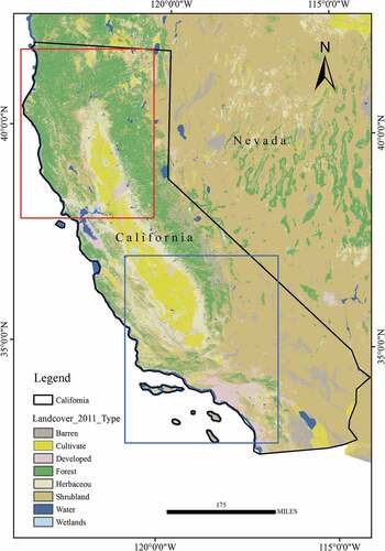
The study areas are located in California, USA (Figure 1), where wildfires frequently occurred in recent decades (Westerling et al. 2006). In 2017, two severe wildfire events happened in the study areas. The one located in northern California started on 8 October, and the other one called “Thomas” fire started on 4 December was mainly located in Ventura County in southern California. The study areas have a typical Mediterranean climate with a wide range of ecosystems including semiarid shrubland, conifer-dominated forests, annual grasslands, croplands, and wetlands. Due to global climate change, extremely dry and erratic rain coupled with the wind in winter make the vegetation ecosystem vulnerable to wildfires (Westerling et al. 2006). Furthermore, the study areas are the most populated regions in the USA, where regular wildfires induced by anthropogenic factors have caused heavy losses to the public and the ecosystems. Wildfires in the study areas usually occur in the dry season from November to February, while some wildfires may even occur in early October or late March and April (Gessner et al. 2015).

Figure 1. The location of the study areas and the land-cover types of California, where wildfires were reported during the 2017 fire season in northern California (red polygon) and in Southern California (blue polygon), respectively. The land-cover map is based on the National Land Cover Database (NLCD) in 2016 (Dewitz 2019). The land cover is grouped into eight general types including Barren, cultivate, Developed, Forest, Herbaceous, Shrubland, Water, and Wetlands.

2.2 Data

2.2.1 Satellite thermal anomaly products

The thermal anomaly products MCD14DL and VNP14IMGT were used to identify the potential BAs in this study. Those products were from the Fire Information for Resource Management System (FIRMS, https://firms.modaps.eosdis.nasa.gov/download/create.php) of Land, Atmosphere Near real-time Capability for EOS (LANCE) National Aeronautics and Space Administration (NASA). It distributes near real-time active fire data within 3 hours of satellite observations from MODIS aboard the Terra and Aqua sensors and VIIRS aboard the joint NASA/NOAA Suomi National Polar orbiting Partnership (Suomi NPP). A contextual algorithm based on the features of strong emission of mid-infrared radiation from fires was adopted to produce those products (Oliva and Schroeder 2015; Giglio et al. 2018). In addition, a confidence level (high, medium, and low) was designated for each active fire point for user’s convenience. The MCD14DL product at a resolution of 1 km derived from MODIS and VNP14IMGT at a resolution of 375 m based on VIIRS are released in shapefile point format with the same projection of WGS84. Both Terra- and Aqua-MODIS instruments observe the entire Earth’s surface 2 times per day. Terra (EOS AM) passes over the equator at approximately 10:30 am and 10:30 pm each day, and the Aqua (EOS PM) passes over the equator at approximately 1:30 pm and 1:30 am. There are at least four daily MODIS observations near the equator, with the number of overpasses increasing toward the poles. Suomi-NPP has a nominal (equator-crossing) overpass time at 1:30 pm and 1:30 am and observes the earth 2 times per day too. In this study, all MCD14DL and VNP14IMGT data in October and December were utilized. Theoretically, there are 6–8 observations per day in California by integrating the MCD14DL and VNP14IMGT thermal anomaly products.

2.2.2 Medium spatial resolution (MSR) satellite images

To accurately monitor the dynamics of BAs by wildfires in near real-time, multiple sources of MSR satellite images are required. Based on the spatial and temporal extents of potential BAs derived from the thermal anomaly products, all freely available MSR satellite images covering the spatial extents of those potential BAs before or on the same date would be collected. In this study, we collected all available cloud-free MSR images of the Advanced Wide Field Sensor (AWiFS) of Resourcesat satellite from the Indian Space Research Organization (ISRO), Landsat OLI, and Sentinel-2A/2B MSI from the Earth Resources Observation and Science (EROS) Center of United States Geological Service (USGS, http://glovis.usgs.gov/) archives. Table 1 shows the spectral band configurations and spatial resolution of these MSR satellite data. As shown in Table 1, Sentinel-2A/B satellites can offer global coverage of observation every 5 days with 10 and 20 m spatial resolution (Navarro et al. 2017). Landsat OLI can provide 30 m spatial resolution observations every 16 days for the same site on the earth, while the Resourcesat1 satellite revisits the same site with 56 m spatial resolution every 5 days. Thus, by integrating Sentinel-2A/B, Landsat, and Resourcesat1 satellite images, there is a great chance that the dynamics of wildfires can be monitored in a near real-time manner with a less than 5-day interval at a spatial resolution finer than 56 m. Table 2 shows the medium spatial resolution images used for extracting the BAs in this study. Table 2 illustrates that southern California wildfires can be monitored at 1-day interval at some specific point of time during their active phase by integrating Resourcesat1 AWIFS, Landsat OLI, and Sentinel-2A/2B MSI images. However, due to constraints of the short duration of wildfires, cloud contaminations, as well as the revisit interval and swath of the satellite images, wildfires in southern California can be monitored with an average 3-day interval.

Table 1. Specifications of the medium spatial resolution sensors used for BA mapping.

	Resourcesat /AWIFS		Landsat/OLI		Sentinel-2A/B
Satellite/Sensor	Bandwidth (µm)	Spatial resolution (m)	Bandwidth (µm)	Spatial resolution (m)	Central Wavelength (µm)	Spatial resolution (m)
Band 1			0.450–0.515 (blue)	30	0.490 (blue)	10
Band 2	0.52–0.59 (green)	56	0.525–0.600 (green)	30	0.560 (green)	10
Band 3	0.62–0.68 (red)	56	0.630–0.680 (red)	30	0.665 (red)	10
Band 4	0.77–0.86 (NIR)	56	0.845–0.885 (NIR)	30	0.842 (NIR)	10
Band 5	1.55–1.70 (SWIR)	56	1.560–1.660 (SWIR1)	30	1.610 (SWIR1)	20
Band 6			2.100–2.300 (SWIR2)	30	2.190 (SWIR2)	20
Number of Bands	4		6		6
Revisit Period (days)	5		16		10

Table 2. Summary of scenes used to detect BAs in California based on the spatial and temporal extensions of daily wildfire points.

	Northern California			Southern California
Wildfire-occurred regions	Satellite/sensor (image acquisition day)
	Resourcesat/AWIFS	Landsat/OLI	Resourcesat /AWIFS	Landsat/OLI	Sentinel-2A/B
Baseline image (pre-fire)	R2AWF_1007_2017244_042_L1T	LC08_044033_20171004_01 T1-SC	R2AWF_1204_2017246_043_L1T	LC08_042036_20171107_01 T1-SC	S2B_20171128_N0206_R070_T11SKU
				LC08_041036_20171202_01 T1-SC	S2A_20171130_N0206_R027_T11SLU
Monitoring image (immediate post-fire)	R2AWF_1012_2017245_043_L1T	LC08_045033_20171027_01 T1-SC	R2AWF_1205_2017251_046_L1T	LC08_041036_20171206_01 T1-SC	S2B_20171205_N0206_R027_T11SKU
	R2AWF_1022_2017247_044_L1T		R2AWF_1214_2017248_042_L1T	LC08_042036_20171209_01 T1-SC	S2B_20171205_N0206_R027_T11SLU
	R2AWF_1031_2017244_042_L1T		R2AWF_1219_2017249_043_L1T	LC08_042036_20171225_01 T1-SC	S2B_20171208_N0206_R070_T11SKU
				LC08_042036_20180126_01 T1-SC	S2B_20171208_N0206_R070_T11SLU

2.2.3 Land-cover map

The National Land Cover Database (NLCD) of 2016 (Dewitz 2019) was used as a land-cover reference to extract wildfire points falling within the vegetation-covered region on the premise that wildfires would burn in the vegetation-covered area. NLCD is an operational land cover monitoring program providing updated land cover and related information for the United States at ~5 year intervals. NLCD 2016 extends temporal coverage to 15 years (2001–2016) to provide nationwide data on land cover and land-cover change at the native 30-m spatial resolution of the Landsat Thematic Mapper (TM).

2.3 Data preprocessing

We merged the MCD14DL and VNP14IMGT thermal anomaly products into a higher temporal frequency fire location database to accurately and rapidly identify potential wildfire points. All Landsat surface reflectance images were obtained from the USGS and corrected from Level 1 T images using the methods described in Vermote et al. (2016). The acquired Level 1 T AWiFS images were converted into surface reflectance images by radiometric correction using ENVI FLAASH (ESRI 2009). Then, the AWiFS surface reflectance images were coregistrated to the Landsat OLI based on 30 ground control points. Moreover, the acquired Level 1C top-of-atmosphere (TOA) reflectance of Sentinel-2A images was transformed into surface reflectance images through atmospheric correction procedure using Sentinel to Correction (Sen2Cor) (Magdalena et al. 2017). As shown in Table 2, the Green, Red, Near-Infrared (NIR) and Short-Wave Infrared (SWIR) bands of OLI, MSI, and AWiFS are nearly consistent in spectral width and central wavelength. In addition, to harmonize the spatial resolution of sentinel-2A and 2B images’ Red, NIR, and SWIR bands into uniform resolution, we resampled images of those bands into 20 m spatial resolution using SNAP (ESA SNAP Homepage 2020).

2.4 Methods

To monitor the progression of BAs by wildfires at medium spatial resolution in near-real time, a two-stage wildfire BA mapping method was proposed in this paper by synergizing multiple high-temporal thermal anomaly products and multi-source MSR satellite images including Sentinel-2A/B MSI, Landsat OLI, and Resourcesat1 AWiFS. The overall workflow is illustrated in Figure 2.

Figure 2. Conceptual representation of the steps for mapping BAs in near real-time using multi-source satellite images.

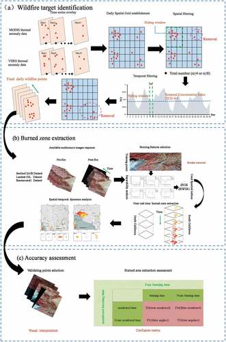
2.4.1 Target zone identification

A variety of thermal anomaly points, such as wildfires, volcanic eruptions, and flare emissions from gas wells, are included in MCD14DL and VNP14IMGT thermal anomaly products. To get actual wildfire points caused by wildfires, other types of thermal anomaly points need to be removed from these thermal anomaly products. In this study, the 30 m NLCD data in 2016 were first used to retain thermal anomaly points located in the vegetated area. Additionally, due to the aggregation in spatial extent and temporal coverage for biomass burning, spatial and temporal filtering procedures were then applied to the merged thermal anomaly product to identify actual wildfire points. The detailed procedures are as follows:

1. Spatial filtering. As wildfires evolve with time, wildfire points would distribute over relatively large spatial extents. The spatial aggregation feature of wildfires was adopted to differentiate wildfire points from other low spatial aggregation thermal anomaly points. To be specific, a 1 km grid was established for the merged thermal anomaly products to measure the spatial aggregation of the thermal anomaly points in each gridded cell. Taking the wind velocity and burning severity into consideration, a 3 km*3 km sliding window was applied to count the maximum number of thermal anomaly points falling in the spatial sliding windows. There are two conditions for the identification of wildfire candidates based on the merged daily thermal anomaly product. One is that the thermal anomaly points falling in the sliding window were observed both in the morning and in the afternoon of a day. The consecutive temporal coverage of those points indicates they are more likely real wildfire points, so the number of thermal anomaly points falling in a sliding window can be relatively small (e.g. a low threshold of n). While the other is that the thermal anomaly points falling in the sliding window were observed either in the morning or in the afternoon of a day. The short duration of those thermal anomaly points indicates they are less likely real wildfire points. To increase the reliability of those points as real wildfire points, the number of points falling in a sliding window should be relatively larger (e.g. a large threshold of n). Once the number of points falling in the sliding window is large enough, they can be recognized as real wildfire candidates. In order to reduce the omission error in identifying actual wildfire points, the thresholds were set as low as possible for both two conditions (i.e. n = 4 and n = 8). The formula is as follows:

(1) $Max\hspace{0.17em}\left\{n_1,n_2,\dots \dots ,n_m\right\}\ge 4\hspace{0.17em}or\hspace{0.17em}Max\hspace{0.17em}\left\{n_1,n_2,\dots \dots ,n_m\right\}\ge 8$(1)

where n₁,n₂, … …, n_m represents the number of thermal anomaly points falling within the spatial sliding window. If the maximum number of thermal anomaly points contained in the sliding window meets the criterion, these thermal anomaly points would be retained as wildfire candidates for further test.

1. Temporal filtering. Although the thresholds were set as low as possible in the spatial filtering procedure, short-duration thermal anomalies that are with high spatial aggregation could be misclassified as real wildfire points. To avoid this kind of misclassification, the temporal-concentration characteristic of biomass burning was utilized to remove the remaining short-term thermal anomaly points. As a result, a modified temporal concentration index (TCI) (shown in Equation(2)(2) $TCI=k\ast n$(2) ) was adopted to determine the temporal aggregation of candidate wildfire points (Liu et al., 2018b). Specifically, a temporal sliding window was set to measure the distribution of retained candidate wildfire points within it. If candidate wildfire points within a spatial sliding window were observed both in the morning and afternoon of a day, the temporal concentration coefficient k was set to 0.1. Otherwise, if candidate wildfire points within the spatial sliding window were observed either in the morning or afternoon of a day, the temporal concentration coefficient was set to 0.05. The TCI was then calculated as the number of candidate wildfire points within the spatial sliding window (n) multiplied by the coefficient. Thus, we applied a fixed threshold of TCI (i.e. TCI = 0.4) to remove the remaining short-duration thermal anomaly points (Figure 2(a)). The TCI is calculated as follows:

(2) $TCI=k\ast n$(2)

where coefficient k is 0.05 or 0.1, and n represents the number of candidate wildfire points within a spatial sliding window. Regarding the dynamic characteristics of wildfires, we ultimately developed a spatial-temporal filtering algorithm, which can rapidly identify actual wildfire points from the daily thermal anomaly product. Finally, 1 km buffer zones outside the filtered wildfire points were developed, and the merged regions of the buffer zones and the areas of wildfire points were set as the BA target zones for immediately collecting MSR images. The details of these filtering processes were shown in Figure 2(a).

2.4.2 Smoke-resistant features extraction for BA mapping

It is crucial to extract effective features for accurately mapping BAs by wildfires. Vegetation indices (VIs) incorporating Short-wave Infrared (SWIR) bands are sensitive to changes in leaf moisture content and shadowing, and VIs incorporating Near-Infrared (NIR) bands are sensitive to changes in plant vigor and canopy density (Moisen et al. 2016). Spectral indices developed by these bands are feasible for BA detection. For example, The Normalized Difference Vegetation Index (NDVI) and differential (pre- minus post-fire) NDVI values have shown a great potential for estimating fire burn severity (Díaz-Delgado, Lloret, and Pons 2003; Hudak et al. 2007; Escuin, Navarro, and Fernández 2008). Meanwhile, many studies reveal that the NBR and dNBR are the most effective spectral indices for mapping BAs of fires (Epting, Verbyla, and Sorbel 2005; Key and Benson 2006; Miller et al. 2009; Veraverbeke et al. 2010). In particular, dNBR is insensitive to atmospheric contamination and it can quantify vegetation removal, charcoal deposition, and reduction of the canopy moisture and canopy shadow, leading to lower NIR and higher SWIR reflectance values, compared to healthy vegetation (Key and Benson 2006).

However, smoke emitted during the active phase of wildfires would obscure the land surface (Smith et al. 2005; Giglio 2007; Roy et al. 2008) and induce much uncertainty in near real-time BA mapping. Spectral indices such as NIR, SWIR, NDVI, NBR, and the differential values of these indices were all selected in this study to test the ability of these indices in discriminating BAs from the unburned areas, nevertheless mitigating the effects of smoke (Table 3). Smoke emitted by wildfires may appear in both BAs and adjacent unburned areas. According to the thickness of smoke appearing within burned areas or outside the burned areas, five scenarios, including burned areas free of smoke (BA) (red dots in Figure 3), unburned areas covered by heavy smoke (HS1) (orange dots in Figure 3), burned areas covered by heavy smoke (HS2) (green dots in Figure 3), unburned areas covered by thin smoke (TS1) (blue dots in Figure 3), and burned areas covered by thin smoke (TS2) (yellow dots in Figure 3), were defined in this study (Figure 3). Training points for each of those scenarios were randomly collected by visual interpretation and the values of selected indices for those points were calculated. The most effective spectral indices were identified by analyzing the statistical differences of the candidate spectral features for the above-mentioned scenarios using the boxplots of the training points. In this study, by a few experiments, 30 training points were selected for each scenario. High spatial resolution images from Google Earth were visually interpreted to verify the land-cover type (vegetation, waterbody, bare ground, developed, and burned area) of those training points during the entire monitoring period (i.e. stable pixels or burned pixels). It is worth noting that, for the convenience of testing and illustrating the ability of those indices in discriminating BAs from other smoke-affected areas, before further analysis was conducted, the values of the selected spectral indices were first normalized to the fixed numerical interval from −1.0 to 1.0.

Figure 3. The spatial distribution of the training points for the “Thomas” wildfires occurred on 4 December in southern California (the Sentinel-2B image was acquired on 8 December, 2017 and is illustrated with band 8/4/3). The left panel with training points of different colors is the zoom-in area in the black rectangle of the top right panel. The training points for each class of burned area, heavy smoke2, heavy smoke1, thin smoke1, and thin smoke2 are rendered in red, green, orange, blue, and yellow colors, respectively.

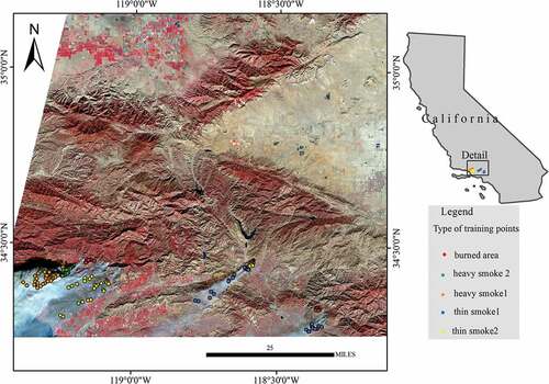
Table 3. Spectral indices used in this study (bands (B) (refer to OLI band order shown in Table 1).

Spectral band/index	Abbreviation	Formula	Notes
NIR Infrared	NIR	B4
Shortwave Infrared	SWIR1	B5	Sensitive to water content
	SWIR2	B6	Sensitive to water content
Normalized Burned Ratio	NBR	(B4-B6)/(B4+ B6)	Sensitive to wildfire effects toecosystems
Normalized Difference Vegetation Index	NDVI	(B4-B3)/(B4+ B3)	Sensitive to green (healthy)vegetation
NIR Difference	dNIR	B4pre-B4post
SWIR Difference	dSWIR1	B5pre-B5post
	dSWIR2	B6pre-B6post
NBR Difference	dNBR	NBRpre-NBRpost
NDVI Difference	dNDVI	NDVIpre-NDVIpost

The F1-score (Cyril and Gaussier 2005) was employed to determine the optimal thresholds of selected spectral indices for BA extraction. To precisely get thresholds for the most effective spectral indices across different sensors, 200 random sample points (100 points for the burned and unburned class, respectively) were generated by referring to the land-cover maps from NLCD as well as the very high spatial resolution images from the Google Earth. The sets of values with the highest F-score for each satellite were retained as the optimal threshold values and applied to BA extraction. The highest F-score could make great tradeoffs between false positives and false negatives for burned and unburned classes and derive great performance not only for overall accuracy but also for individual classes. The F-score is calculated as follows:

(3) $F1=\frac{TP}{TP+\frac{1}{2}\left(FP+FN\right)}$(3)

where TP, FN, and FP represent true positive (correctly classified burned points), false negative (burned points classified as unburned points), and false positive (unburned points misclassified as burned points), respectively.

2.4.3 Near real-time wildfire BA extraction

Once the spatial extents of daily wildfire points were identified, 1 km buffer zones were established for the spatial extents of wildfire points. Then, the spatial extents of daily wildfire points merged with the butter zones were taken as actual target zones. Based on the spatial extents of daily target zones, all available images from Sentinel 2A/B, Landsat OLI, and Resourcesat AWiFS were collected immediately on the same date. Simultaneously, all available pre-wildfire baseline images were also collected. Since the most smoke-resistant spectral indices were selected, as well as the optimal thresholds of these indices for each satellite were identified, all these indices would be calculated for the collected MSR images. As a result, the BAs can be extracted instantly and continuously as wildfires evolve. If MSR images are sufficient, the spatial and temporal dynamics of wildfires can be monitored with a daily frequency by the proposed two-stage method.

2.4.4 Accuracy assessment

In practice, there is no other independent BA product with the same temporal and spatial resolution for validating the performance of the proposed BA mapping method. In order to assess the performance of the two-stage near real-time wildfire BA mapping developed by Olofsson et al. method, we selected spatially random samples on each specific date by following the good practice (2014) and labeled the samples through visual interpretation based on the clear MSR images. Meanwhile, the burned dates detected by the two-stage near real-time BA mapping method for these validation samples were also recorded. A confusion matrix generated by the detected and labeled classes was applied to evaluate the accuracies of extracted BAs. Because the area of detected BA on each monitoring date is less than 1% of the area of the entire California, as suggested by Olofsson (2014), the sample size for each stratum (date) was set between 50 and 100. As a result, a total of 260 samples within BAs and 729 samples within unburned areas were selected for the northern California wildfires, and 460 samples within BAs and 484 samples within unburned areas were selected for southern California wildfires for accuracy assessment.

3. Results

3.1 Spatio-temporal dynamics of wildfire points

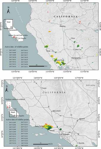
As is shown in Figure 4a, identified actual wildfire points in northern California continued burning from 7 through 19 October and from 29 through 31 October. The detected wildfire points were widely distributed over the whole study area. Among them, nine major BAs were located at the northwest and the edge of the central plain of California, where land-cover types of these BAs were dominated by cultivated land, forest, herbaceous, and shrubland. The spatial distribution of the identified actual wildfire points in southern California continuously burning from 5 through 25 December is presented in Figure 4b. Unlike the widely distributed wildfire points in northern California, wildfire points in southern California were more spatially concentrated. The major wildfire points were located in southwest California, which was reported as the “Thomas” wildfire.

Figure 4. Spatial and temporal distribution of the detected wildfire points in (a) northern and (b) southern California. Figure (a) and (b) are the zoom-in areas in the black rectangles of the entire California in the inset maps, respectively. Wildfire points detected on the different dates from 7to31 October are rendered in different colors from dark green to red. Wildfire points that are not illustrated by the current figure (a or b) are rendered in the red color in the inset maps of the entire California illustrated on the left side of each figure.

3.2 The effectiveness of spectral indices

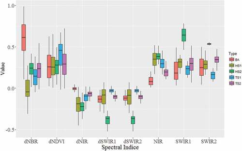
To test the ability of the indices in discriminating BAs from the unburned areas and mitigating the effects of smoke, the boxplots for the values of candidate spectral indices of the five scenarios are presented in Figure 5. In this study, the burned areas free from smoke (BA), burned areas covered by heavy smoke (HS2), and burned areas covered by thin smoke (TS2) need to be correctly extracted. Figure 5 shows that the NIR band can separate BAs free from smoke from other smoke-covered areas. SWIR1 and SWIR2 can discriminate BAs covered by heavy smoke from BAs free from smoke and other smoke-covered areas. Meanwhile, the dNIR and dNBR can also separate BAs free from smoke from other smoke-covered areas. The dSWIR1 and dSWIR2 also show great potential in distinguishing BAs covered by heavy smoke from BAs free from smoke and other smoke-related areas, but they cannot separate BAs covered by thin smoke (TS2) from other scenarios well. Due to the penetration capability of the SWIR band, the burned areas covered by thin smoke (TS2) can be partially extracted by using dSWIR1. To keep the spectral indices for extracting BA consistent across different sensors and improve computing efficiency, the dNBR and dSWIR1 were selected to extract the BAs of wildfires.

Figure 5. Boxplots of different spectral indices’ values under each scenario of the “Thomas” wildfire that occurred on 5 December based on Sentinel-2A/2B sensors. The spectral indices form roughly 3 groups and the differences within these groups are not particularly significant. The dNBR, dNIR, and NIR show great capability in distinguishing BA from other types, while dSWIR1, dSWIR2, SWIR1, and SWIR2 both exhibit great potential in discriminating HS2 from other classes. However, there is no spectral index that shows a prominent advantage in separating TS2 from other classes (1 represents samples falling outside BA, 2 represents samples falling within BA. BA, HS, and TS are the abbreviation of burned area, Heavy smoke area, and Thin smoke area, respectively).

3.3 Optimal Thresholds selection

By analyzing the boxplots shown in Figure 5, we can approximately determine the potential optimal thresholds for Sentinel-2A/B images in accurately identifying BAs, which are 0.42 and −0.2 for the dNBR and dSWIR1, respectively. When the value of dNBR is greater than 0.42 and the value of dSWIR1 is less than −0.2 simultaneously, the BAs can be extracted for Sentinel-2A/B images. However, these values may not be the optimal ones. Thus, to get the optimal thresholds, we performed a further test on the candidates of the optimal dNBR and dSWIR1 thresholds for the Sentinel-2A/B images. 0.39, 0.40, 0.41, 0.42, 0.43, 0.44, 0.45 for dNBR, −0.23, −0.22, −0.21, −0.20, −0.19, −0.18, −0.17 for dSWIR1 were tested on the 200 samples described in section 2.4.2 by calculating the F-score for each threshold combination. A total of 49 sets of thresholds were tested on the 200 samples (pixels) to specify the optimal threshold combination. As illustrated in Table 4, the optimal threshold values with the highest F-score (0.855) were 0.42 for dNBR and −0.23 for dSWIR1. Notably, we also performed a visual check on the change maps derived using different threshold combinations in addition to calculating the F1-score for those samples. Similarly, by checking a variety of typical unburned areas and burned areas, the optimal threshold combination also come up with the most satisfactory results when compared to those of other threshold combinations. Using the same method, the optimal threshold values of dNBR and dSWIR1 for Landsat OLI (0.44 and −0.22) and Resourcesat AWiFS (0.40 and −0.21) were also determined.

Table 4. F1-score of each set of candidate threshold values of dNBR and dSWIR for the 200 samples (100 unburned samples and 100 burned samples) for the “Thomas” wildfire occurred on 5 December based on the Sentinel-2B image.

	dSWIR1
dNBR	0.39	0.40	0.41	0.42	0.43	0.44	0.45
−0.23	0.806	0.828	0.841	0.855	0.825	0.832	0.849
−0.22	0.846	0.837	0.832	0.845	0.842	0.846	0.814
−0.21	0.828	0.828	0.834	0.825	0.821	0.835	0.816
−0.2	0.825	0.806	0.835	0.840	0.839	0.845	0.811
−0.19	0.829	0.811	0.843	0.843	0.830	0.830	0.829
−0.18	0.838	0.811	0.830	0.840	0.818	0.811	0.827
−0.17	0.828	0.847	0.835	0.821	0.807	0.832	0.827

3.4 Near real-time wildfire BAs extraction

3.4.1 Spatial dynamics of BAs

Figure 6a illustrates that major BAs were mainly distributed at the edge of the central agricultural area in northern California. Other small BAs were scattered in the north and the east of northern California. The BAs spreading from the southwest toward the northeast of northern California were extracted on 11, 12, 22, and 31 October, respectively. The detected BAs have been decreasing since 22 October and the biggest BA was extracted on 12 October. Meanwhile, there were only three small burned patches detected in northern California on 31 October. In general, the proposed method can identify the BAs only with a 3-day delay and consecutively monitor the dynamics of northern California wildfires with a less than 5-day interval. An exception is for the time interval between 12 and 19 October, when a 7-day delay appeared due to lacking clear MSR observations.

Figure 6. The spatial distribution and monitoring time of BAs in (a) northern and (b) southern California. (a) and (b) show the detected BAs of northern and southern California wildfires, respectively. The top panels display the zoom-in BAs in black rectangles in the insets for the entire California. The bottom panels display the zoom-in BAs in the green and yellow rectangles in the insets for the entire California shown in the top right of the top panels. The detected BAs at different times are rendered in different colors from yellow to red.

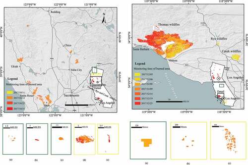
Figure 6b shows that the BAs in southern California were spatially concentrated. The available MSR images were mainly from the Landsat OLI and Sentinel-2A/B sensors, which can fully cover the main BAs (“Thomas” fire) in one or two scenes. Because one Resourcesat1 AWiFS image can cover the entire BAs of southern California, the dynamics of southern California wildfires were monitored with higher temporal frequency than that of northern California. The main wildfire event known as “Thomas” started in Ventura County on 4 December and moved toward the northwest of California. As shown in Figure 6b, our method can map BAs in southern California only with a 1-day delay. Better than the performance in northern California, our method can monitor the progression of BAs of wildfires with a 1-day interval at the early stage of the wildfires in southern California. Due to the limitation of available MSR images, the BAs were extracted with a 5-day and 6-day interval from 9 to 19 December and 19 to 25 December, respectively.

Figures 6 and Figure 4 show high consistency in the spatial extents of BAs, which to some extent indicates that the accuracy of identified wildfire points by spatial and temporal sliding windows is high. Because available images for northern California wildfires are mainly from Resourcesat1 AWiFS, available images for southern California wildfires are mainly from the Sentinel-2A/B MSI and Landsat OLI, the detected BAs for southern California wildfires (Figure 6b) exhibited more spatial details than those for northern California wildfires (Figure 6a). In addition, the BAs of northern California wildfires were more spatially scattered than those of southern California.

3.4.2 Temporal dynamics of BAs

Figure 7 illustrates that the BAs of wildfires that occurred in northern California increased with time and reached the largest extent on 12 October with an area of 502.22 km². Then, the BAs decreased with time and reached the smallest extent of the entire wildfire event on 31 October. The total BA of northern California wildfires was 540.75 km². In contrast, the BA at each monitoring time in southern California varied greatly over time, and the overall trend of BA was decreasing. Due to the limitation of available MSR images, only a small portion of BA besides the “Thomas” wildfire can be detected on 6 December. Thus, the BA of this date was extremely low. The BA of southern California wildfires was 846.65 km², which was greater than that of northern California. The BAs of the forest, herbaceous, and shrubland for wildfires in northern California were 281.23, 154.73 and 87.99 km², respectively, which were smaller than these in southern California. A total of 16.80 km² of cultivated land was burned in northern California wildfires, while there was no burned cultivated land for southern California wildfires (Table 5).

Figure 7. BA at each monitoring time in (a) northern and (b) southern California. Each bar in Figure 7 represents the BA (left axis) at each monitoring time, and the solid black line denotes the cumulative BA (right axis) at each monitoring date (solid square) as wildfires evolve.

Table 5. The total BA for each vegetation type in California.

	Burned land-cover type	Burned area (km^2)
		Northern California	Southern California	Total area (km^2)
	Forest	281.23	348.51	629.74
	Herbaceous	154.73	168.81	323.54
	Shrub	87.99	329.33	417.32
	Cultivated	16.80		16.80
Total area (km^2)		540.75	846.65	1387.4

3.5 Extraction accuracy of BA

As shown in Table 6, the Overall accuracy (OA) for detected BAs in southern California is 0.85, which is very close to that of northern California (0.84). However, the Producer’s accuracies (PAs) of BAs in southern California are almost all higher than these of northern California for the same satellite, which indicates that the omission errors of BAs of southern California are lower than these of northern California. The user’s accuracies (UA) of BAs at each monitoring time in northern California are 0.74 for Landsat OLI, and 0.70, 0.62, and 0.66 for Resourcesat AWiFS, respectively. In southern California, the UAs of BAs extracted by the Sentinel-2A/B are 0.90 and 0.87, respectively, while the UAs of BAs extracted by Landsat OLI are 0.83, 0.80, and 0.80, respectively. Both UAs of BAs extracted by Sentinel-2 and Landsat OLI are higher than those extracted by Resourcesat AWiFS. These results indicate that while the UA for each of the BAs in California is relatively high, satellite images with higher spatial resolution could achieve higher UAs for BAs.

Table 6. Classification accuracy of BAs by wildfire from our automated monitoring method.

Wildfires burned region	Error matrix									Accuracy
	Detected burning time/sensor	Real burning time/sensor
Northern California		1011/L	1012/R	1022/R	1031/R	unburned	Line total				PA	UA	OA
	1011/L	42				15	57				0.84	0.74	0.84
	1012/R		77			33	110				0.77	0.70
	1022/R			44		27	72				0.73	0.62
	1031/R				37	19	56				0.74	0.66
	unburned	8	23	16	13	635	695				0.87	0.91
	Column total	50	100	60	50	729
Southern California		1205/S	1206/L	1208/S	1209/L	1214/R	1219/R	1225/L	unburned	Line total	PA	UA	OA
	1205/S	78							8	86	0.91	0.90	0.85
	1206/L		43						9	52	0.86	0.83
	1208/S			71					11	82	0.89	0.87
	1209/L				54				13	67	0.83	0.80
	1214/R					56			15	71	0.80	0.79
	1219/R						49		12	61	0.82	0.80
	1225/L							43	9	52	0.86	0.80
	unburned	7	7	9	12	14	11	7	407	475	0.84	0.83
	Column total	85	50	80	65	70	60	50	484

aR, L, and S represent Resourcesat AWiFS, Landsat OLI, and Sentinel-2A/B image, respectively.

4. Discussion

Near real-time BA mapping is vital to timely wildfire response as wildfires have frequently occurred worldwide and threatened human life over the past years (Chuvieco et al. 2019). In this study, we proposed a two-stage near real-time BA mapping approach using multiple remote-sensing data. The thermal anomaly products derived from high revisiting period sensors including MODIS and VIIRS were first used to identify wildfires and potential BAs. Then, images from multiple MSR sensors such as Sentinel 2A/2B, Landsat OLI, and Resourcesat AWiFS were synergized for near real-time BA mapping at a fine spatial resolution. The method was applied in California where two wildfires occurred in northern and southern California in 2017. The results show that the proposed method is accurate for BA mapping with an overall accuracy of 0.84 and 0.85 for wildfires in northern and southern California, respectively. The extracted BAs depict the explicit spatial details and temporal dynamics of the two big wildfire events that occurred in California in 2017. The proposed method can monitor BAs with an average 3.5-day interval and 4-day latency for the wildfires in southern California, and an average 3-day interval and sub-daily latency for wildfires in northern California, respectively. It made a great advance in near real-time BA mapping in terms of spatial details, temporal frequency, and latency.

Specifically, due to the trade-off between spatial and temporal resolutions, single satellite data are insufficient to provide the spatio-temporal dynamics of BAs by wildfires. Although moderate sensors can capture explicit spatial details of BAs, due to the relatively long revisit interval and the narrow swath of these sensors, the capability and efficiency for timely finding wildfires and mapping BAs using only MSR sensors are extremely low. Thus, it is infeasible to timely locate where the burns are and when the burns start. However, satellite data with high-temporal resolution and wide spatial coverage such as MODIS and VIIRS can monitor the progression of wildfires with a sub-daily interval (less than 12 h) and hours delay (less than 3 h). Thus, it is possible to quickly target the potential BAs by using the spatial and temporal sliding-window-based method (the first stage of our two-stage method) only with hours of delay and continuously monitor the evolving dynamics of BAs by wildfires with a sub-daily interval. Furthermore, the subsequent BA mapping procedure (the second stage of our two-stage method) can quickly start by efficiently collecting all available MSR images pre- and post-wildfires only covering the spatial extents of the potential BAs. In conclusion, all merits mentioned above make the two-stage BA mapping method a quick and efficient way for near real-time BA mapping. Here, the meaning embedded in the “quickly” in this study lies in timely targeting the potential BAs by combining multiple high temporal resolution sensors, and the meaning of “efficient” lies in improving the monitoring temporal frequency and spatial resolution of BAs by synergizing all freely available MSR images for the targeted potential BAs

Even though the potential BAs can be detected with hours of delay and can be monitored at a sub-daily interval, the big challenge for achieving near real-time or even real-time BA mapping with the proposed two-stage method is the accessibility of clear, free MSR images. In practice, because of clouds and cloud shadows, the availability of clear MSR data is sometimes limited. As a result, the BA mapping frequency may be reduced. However, synergizing observations from more and more multiple MSR sensors can overcome this shortcoming and timely monitor the progression of wildfires (Hilker et al. 2009a; Wulder et al. 2010; Jian and Roy 2017; Wulder et al. 2018). As for wildfires in northern California (Figure 6a), there was only one Landsat-8 available at the early stage of the active fire in northern California and no available Sentinel-2 image during the active phase of wildfires. Using Landsat-8 alone, the BA mapping procedure will start 2 days after wildfires had started. If only relying on observations from Resourcesat AWiFS, we can trace the dynamics of BAs with 4 days delay. However, by synergizing observations from Resourcesat AWiFS and Landsat-8, the BAs of wildfires in northern California can be monitored with 2 days delay and an average 3.5-day interval. Wildfires in southern California were in a similar situation (Figure 6b). If relying on three observations from Landsat-8 alone, the BA mapping procedure could begin one day after the wildfires had started. Similarly, if only relying on Sentinel-2 data, the BA mapping procedure would start one day after the wildfires had started and be restricted to two discrete dates at the very early stage of the wildfires in southern California. If only using Resourcesat AWiFS data, the BAs of wildfires in southern California can be traced with 9 days delay and in the middle stage of them. However, by synergizing observations from Resourcesat AWiFS, Landsat-8, and Sentinel-2A/2B, the BAs of wildfires in southern California can be monitored with a 1-day delay and an average 3-day interval. Thus, using observations from multiple MSR sensors can greatly improve the monitoring frequency and reduce the response latency for mapping the dynamics of BAs by wildfires. Additionally, as is shown in Figure 6, the higher the spatial resolution of the images used for BA mapping, the more spatial details of the detected BAs. Using only observations from Resourcesat AWiFS would lead to higher omission and commission errors for BAs. This limitation can be avoided by using data from other high spatial resolution sensors (e.g. Landsat and Sentinel data).

Our method is not restricted to any satellite. More and more freely accessible satellite data helpful for creating denser time-series stacks can be employed for real-time mapping BAs of the evolving wildfires. At the first stage of our method, other coarse-resolution sensors such as GOES, Himawari-8, and Meteosat could also be combined with MODIS and VIIRS to identify the potential BAs with even minutes delay and interval. At the second stage of our method, high spatial resolution (HSR) sensors such as GF-1, GF-2, HJ-1/2, ZY3-02 from China, and commercial satellites such as worldview-3/4, GeoEye-1, QuikBird, and PlanetScope could also be coordinated with MSR images such as Landsat, Sentinel-2, and Resourcesat AWiFS to fulfill real-time BA mapping at the regional and global scales. Thus, the proposed near real-time BA mapping method can be applied to detect a wide range of abrupt change events with unprecedented temporal frequency and finer spatial resolution.

The proposed method shows prominent advantages in the following aspects. First, by synergizing sensors with high temporal frequency and large coverage, we can timely target wildfires at the regional or global scales. Then, as soon as potential BAs are identified, all freely available MSR sensors can be timely and efficiently collected at places covering these BAs. Finally, explicit spatial details of wildfires can be mapped by synergizing MSR sensors. However, the two-stage method also exposes some limitations. First, in the first stage of the method, we used the thermal anomaly products from MODIS and VIIRS to quickly target the potential BAs of wildfires without carefully considering the accuracies of these products. Due to the coarse spatial resolutions of these products, false alarms and undetected small or even medium wildfires lead to much uncertainty in the detection of BAs in the second stage of the two-stage method. Second, in the second stage of our method, as illustrated in Figure 5, BAs covered by thin smoke (TS2) cannot be clearly discriminated from other scenarios by dNBR and dSWIR1. Other useful spectral indices such as NBI (Mpakairi, Lynnet Kadzunge, and Ndaimani 2020) and RdNBR (Miller et al. 2009) that were not used in this study should be tested in further study to increase the possibility of these indices in distinguishing all burned scenarios from the unburned ones. In addition, we mapped the spatial extents of wildfires based on the absolute thresholds of selected spectral indices without considering their burn severity in the second stage of the method. Burn severity, which refers to the degree of identified changes from burning, somewhat denotes the uncertainty of the extents of BAs as quantified by scaled spectral indices, such as dNBR (Key and Benson 2006; Miller et al. 2009; Mallinis, Mitsopoulos, and Chrysafi 2017). Therefore, further study should consider incorporating the burn severity into the two-stage framework to get integrated information about BAs. Finally, due to lacking other independent BA products with the same time frequency and spatial resolution, validating the performance of the proposed method is also a challenge (Justice et al. 2000). Previous studies have mostly focused on accurately extracting BAs by wildfires based on post-wildfire images (Roy et al. 2002; Pérez-Cabello et al. 2012; Mitri and Gitas 2013), the evolving dynamics of BAs were seldom referred to. Thus, an intercomparison of accuracy for extracted BAs between the two-stage method and other independent reference data was not implemented in this study.

5. Conclusions and recommendations

We proposed a two-stage method based on multi-sensor remote-sensing data for near real-time BA mapping. Thermal anomaly products from high temporal resolution sensors including MODIS and VIIRS were first used to identify wildfires and potential BAs. Then, multiple MSR sensors including Sentinel-2A/2B, Landsat OLI, and Resourcesat AWiFS were synthesized for extracting BAs with more spatial details in near real-time. The proposed method was applied in California, USA where wildfires occurred in northern and southern California in 2017. The results showed that the proposed method was accurate for BA mapping with an overall accuracy of 0.84 and 0.85 for wildfires in northern and southern California, respectively. The proposed method can monitor BAs with an average 3.5-day interval and 4-day latency for the wildfires in southern California, and an average 3-day interval and sub-daily latency for wildfires in northern California, respectively. The proposed method overcomes the shortcomings in BA mapping based on only single satellite data, which are the sensors with short revisit periods fail to provide explicit spatial details of wildfires (e.g. small and patchy fires: <100 ha; Roteta et al. 2019), while the medium resolution sensors are not sufficient to timely locate wildfires that may occur at any time and any place over the world. Both groups of sensors cannot timely identify wildfires while accurately mapping BAs of wildfires. Our two-stage method can be taken as a vital advance for near real-time BA mapping by synergizing remote-sensing data from multiple high temporal frequency and all free MSR sensors. With more and more MSR and HSR satellite data freely open to the public, combining them to build denser time series for real-time detection of a variety of abrupt land surface change events at the regional and global scales is becoming more realizable than before. While the proposed two-stage method provides an effective way to continuously monitor BAs in near real-time, the performance of this method could be improved by incorporating the burn severity information in the BA detection. In addition, it is valuable to implement the proposed two-stage BA mapping method on the planetary-scale cloud platform such as Google Earth Engine (GEE) for more efficient near real-time mapping of BAs globally.

Acknowledgements

We are thankful for the freely accessible Landsat OLI, Sentinel-2A/2B, and Resourcesat AWiFS data by USGS and the thermal anomaly products MCD14DL and VNP14IMGT from FIRMS by NASA. We would like to thank the reviewers for their constructive comments during the revision of this paper.

Disclosure statement

No potential conflict of interest was reported by the author(s).

Additional information

Funding

This study was jointly supported by the National Natural Science Foundation of China (41871232) and the National Key Research and Development Program of China [2016YFB0501502].

References

- AghaKouchak, A., L. S. Huning, F. Chiang, M. Sadegh, F. Vahedifard, O. Mazdiyasni, H. Moftakhari, and I. Mallakpour. 2018. “How Do Natural Hazards Cascade to Cause Disasters?” Nature 561 (7724): 458–460. doi:10.1038/d41586-018-06783-6.
- Alonso-Canas, I., and E. Chuvieco. 2015. “Global Burned Area Mapping from ENVISAT-MERIS and MODIS Active Fire Data.” Remote Sensing of Environment 163 (June): 140–152. doi:10.1016/j.rse.2015.03.011.
- Ban, Y., P. Zhang, A. Nascetti, A. R. Bevington, and M. A. Wulder. 2020. “Near Real-Time Wildfire Progression Monitoring with Sentinel-1 SAR Time Series and Deep Learning.” Scientific Reports 10 (1): 1322. doi:10.1038/s41598-019-56967-x.
- Barbosa, P. M., D. Stroppiana, J.-M. Grégoire, and J. Miguel Cardoso Pereira. 1999. “An Assessment of Vegetation Fire in Africa (1981-1991): Burned Areas, Burned Biomass, and Atmospheric Emissions.” Global Biogeochemical Cycles 13 (4): 933–950. doi:10.1029/1999GB900042.
- Bar, S., B. Ranjan Parida, G. Roberts, A. Chandra Pandey, P. Acharya, and J. Dash. 2021. “Spatio-Temporal Characterization of Landscape Fire in Relation to Anthropogenic Activity and Climatic Variability over the Western Himalaya, India.” GIScience & Remote Sensing 58 (2): 281–299. doi:10.1080/15481603.2021.1879495.
- Boschetti, L., P. A. Brivio, and J. M. Gregoire. 2003. “The Use of Meteosat and GMS Imagery to Detect Burned Areas in Tropical Environments.” Remote Sensing of Environment 85 (1): 78–91. doi:10.1016/S0034-4257(02)00189-X.
- Bowman, D. 2018. “Wildfire Science Is at a Loss for Comprehensive Data.” Nature 560 (7716): 7. doi:10.1038/d41586-018-05840-4.
- Briones-Herrera, C. I., D. José Vega-Nieva, N. Angélica Monjarás-Vega, J. Briseño-Reyes, P. Marcelo López-Serrano, J. Javier Corral-Rivas, E. Alvarado-Celestino, et al. 2020. “Near Real-Time Automated Early Mapping of the Perimeter of Large Forest Fires from the Aggregation of VIIRS and MODIS Active Fires in Mexico.” Remote Sensing 12 (12): 2061. doi:10.3390/rs12122061.
- Chéret, V., and J. P. Denux. 2011. “Analysis of MODIS NDVI Time Series to Calculate Indicators of Mediterranean Forest Fire Susceptibility.” GIScience & Remote Sensing 48 (2): 171–194. doi:10.2747/1548-1603.48.2.171.
- Chuvieco, E., F. Mouillot, G. R. van der Werf, J. San Miguel, M. Tanasse, N. Koutsias, M. García, et al. 2019. “Historical Background and Current Developments for Mapping Burned Area from Satellite Earth Observation.” Remote Sensing of Environment 225 (May): 45–64. doi:10.1016/j.rse.2019.02.013.
- Crowley, M. A., J. A. Cardille, J. C. White, and M. A. Wulder. 2019. “Multi-Sensor, Multi-Scale, Bayesian Data Synthesis for Mapping within-Year Wildfire Progression.” Remote Sensing Letters 10 (3): 302–311. doi:10.1080/2150704X.2018.1536300.
- Cyril, G., and E. Gaussier. 2005. “A Probabilistic Interpretation of Precision, Recall and F-Score, with Implication for Evaluation.” In Advances in Information Retrieval, edited by D. E. Losada and J. M. Fernández-Luna, Vol. 3408 345–359. Lecture Notes in Computer Science. Berlin, Heidelberg: Springer Berlin Heidelberg. 10.1007/978-3-540-31865-1_25.
- Dewitz, J., 2019, “Data from U.S. Geological Survey .” National Land Cover Database (NLCD) 2016 Products (ver. 2.0, July 2020). Accessed 24 July 2020. 10.5066/P96HHBIE.
- Díaz-Delgado, R., F. Lloret, and X. Pons. 2003. “Influence of Fire Severity on Plant Regeneration by Means of Remote Sensing Imagery.” International Journal of Remote Sensing 24 (8): 1751–1763. doi:10.1080/01431160210144732.
- Dwyer, E., S. Pinnock, J. M. Gregoire, and J. M. C. Pereira. 2000. “Global Spatial and Temporal Distribution of Vegetation Fire as Determined from Satellite Observations.” International Journal of Remote Sensing 21 (6–7): 1289–1302. doi:10.1080/014311600210182.
- Epting, J., D. Verbyla, and B. Sorbel. 2005. “Evaluation of Remotely Sensed Indices for Assessing Burn Severity in Interior Alaska Using Landsat TM and ETM+.” Remote Sensing of Environment 96 (3–4): 328–339. doi:10.1016/j.rse.2005.03.002.
- ESA SNAP Homepage (2020). Accessed 08 september 2020. http://step.esa.int/main/toolboxes/snap
- Escuin, S., R. Navarro, and P. Fernández. 2008. “Fire Severity Assessment by Using NBR (Normalized Burn Ratio) and NDVI (Normalized Difference Vegetation Index) Derived from LANDSAT TM/ETM Images.” International Journal of Remote Sensing 29 (4): 1053–1073. doi:10.1080/01431160701281072.
- ESRI. 2009. “Atmospheric Correction Module” Accessed August 2009. http://www.rsinc.com/envi/flaash.asp
- Eva, H., and E. F. Lambin. 1998. “Burnt Area Mapping in Central Africa Using ATSR Data.” International Journal of Remote Sensing 19 (18): 3473–3497. doi:10.1080/014311698213768.
- Florath, J., and S. Keller. 2022. “Supervised Machine Learning Approaches on Multispectral Remote Sensing Data for a Combined Detection of Fire and Burned Area.” Remote Sensing 14 (3): 657. doi:10.3390/rs14030657.
- Fraser, R. H., R. J. Hall, R. Landry, T. Lynham, D. Raymond, B. Lee, and Z. Li. 2004. “Validation and Calibration of Canada-Wide Coarse-Resolution Satellite Burned-Area Maps.” Photogrammetric Engineering and Remote Sensing 70 (4): 451–460. doi:10.14358/PERS.70.4.451.
- Frazier, R. J., N. C. Coops, M. A. Wulder, T. Hermosilla, and J. C. White. 2018. “Analyzing Spatial and Temporal Variability in Short-Term Rates of Post-Fire Vegetation Return from Landsat Time Series.” Remote Sensing of Environment 205 (February): 32–45. doi:10.1016/j.rse.2017.11.007.
- Fuller, D. O. 2000. “Satellite Remote Sensing of Biomass Burning with Optical and Thermal Sensors.” Progress in Physical Geography 24 (4): 543–561. doi:10.1191/030913300701542787.
- Gessner, U., K. Knauer, C. Kuenzer, and S. Dech. 2015. “Land Surface Phenology in a West African Savanna: Impact of Land Use, Land Cover and Fire.” In Remote Sensing Time Series, edited by C. Kuenzer, S. Dech, and W. Wagner, Vol. 22 203–223. Remote Sensing and Digital Image Processing. Cham: Springer International Publishing. 10.1007/978-3-319-15967-6_10.
- Giglio, L. 2007. “Characterization of the Tropical Diurnal Fire Cycle Using VIRS and MODIS Observations.” Remote Sensing of Environment 108 (4): 407–421. doi:10.1016/j.rse.2006.11.018.
- Giglio, L., L. Boschetti, D. P. Roy, M. L. Humber, and C. O. Justice. 2018. “The Collection 6 MODIS Burned Area Mapping Algorithm and Product.” Remote Sensing of Environment 217 (October): 72–85. doi:10.1016/j.rse.2018.08.005.
- Hermosilla, T., M. A. Wulder, J. C. White, N. C. Coops, G. W. Hobart, and L. B. Campbell. 2016. “Mass Data Processing of Time Series Landsat Imagery: Pixels to Data Products for Forest Monitoring.” International Journal of Digital Earth 9 (11): 1035–1054. doi:10.1080/17538947.2016.1187673.
- Hilker, T., M. A. Wulder, N. C. Coops, J. Linke, G. McDermid, J. G. Masek, F. Gao, and J. C. White. 2009a. “A New Data Fusion Model for High Spatial- and Temporal-Resolution Mapping of Forest Disturbance Based on Landsat and MODIS.” Remote Sensing of Environment 113 (8): 1613–1627. doi:10.1016/j.rse.2009.03.007.
- Hilker, T., M. A. Wulder, N. C. Coops, N. Seitz, J. C. White, F. Gao, J. G. Masek, and G. Stenhouse. 2009b. “Generation of Dense Time Series Synthetic Landsat Data through Data Blending with MODIS Using a Spatial and Temporal Adaptive Reflectance Fusion Model.” Remote Sensing of Environment 113 (9): 1988–1999. doi:10.1016/j.rse.2009.05.011.
- Hudak, A. T., P. Morgan, M. J. Bobbitt, A. M. S. Smith, S. A. Lewis, L. B. Lentile, P. R. Robichaud, J. T. Clark, and R. A. McKinley. 2007. “The Relationship of Multispectral Satellite Imagery to Immediate Fire Effects.” Fire Ecology 3 (1): 64–90. doi:10.4996/fireecology.0301064.
- Humber, M. L., L. Boschetti, L. Giglio, and C. O. Justice. 2019. “Spatial and Temporal Intercomparison of Four Global Burned Area Products.” International Journal of Digital Earth 12 (4): 460–484. doi:10.1080/17538947.2018.1433727.
- Jian, L., and D. Roy. 2017. “A Global Analysis of Sentinel-2A, Sentinel-2B and Landsat-8 Data Revisit Intervals and Implications for Terrestrial Monitoring.” Remote Sensing 9 (9): 902. doi:10.3390/rs9090902.
- Justice, C., A. Belward, J. Morisette, P. Lewis, J. Privette, and F. Baret. 2000. “Developments in the ‘Validation’ of Satellite Sensor Products for the Study of the Land Surface.” International Journal of Remote Sensing 21 (17): 3383–3390. doi:10.1080/014311600750020000.
- Key, C., and N. Benson. 2006. “Landscape Assessment: Ground Measure of Severity, the Composite Burn Index; and Remote Sensing of Severity, the Normalized Burn Ratio.” In FIREMON: Fire Effects Monitoring and Inventory System, edited by D. Lutes, R. Keane, J. Caratti, C. Key, N. Benson, and L. Gangi, 219–279. Technical Report RMRS-GTR-164-CD. Fort Collins, CO: USDA Forest Service, Rocky Mountains Research Station General.
- Liu, X., H. Binbin, X. Quan, M. Yebra, S. Qiu, C. Yin, Z. Liao, and H. Zhang. 2018a. “Near Real-Time Extracting Wildfire Spread Rate from Himawari-8 Satellite Data.” Remote Sensing 10 (10): 1654. doi:10.3390/rs10101654.
- Liu, Y., H. Chuanmin, W. Zhan, C. Sun, B. Murch, and M. Lei. 2018b. “Identifying Industrial Heat Sources Using Time-Series of the VIIRS Nightfire Product with an Object-Oriented Approach.” Remote Sensing of Environment 204 (January): 347–365. doi:10.1016/j.rse.2017.10.019.
- Magdalena, M.-K., B. Pflug, J. Louis, V. Debaecker, U. Müller-Wilm, and F. Gascon. 2017. “Sen2Cor for Sentinel-2.” In Image and Signal Processing for Remote Sensing XXIII, edited by L. Bruzzone, F. Bovolo, and J. A. Benediktsson, 37–48. Bellingham, WA: SPIE. doi:10.1117/12.2278218.
- Mallinis, G., I. Mitsopoulos, and I. Chrysafi. 2017. “Evaluating and Comparing Sentinel 2A and Landsat-8 Operational Land Imager (OLI) Spectral Indices for Estimating Fire Severity in a Mediterranean Pine Ecosystem of Greece.” GIScience & Remote Sensing 55 (1): 1–18. doi:10.1080/15481603.2017.1354803.
- Mandanici, E., and G. Bitelli. 2016. “Preliminary Comparison of Sentinel-2 and Landsat 8 Imagery for a Combined Use.” Remote Sensing 8 (12): 1014. doi:10.3390/rs8121014.
- McCarley, T. R., A. M. S. Smith, C. A. Kolden, and J. Kreitler. 2018. “Evaluating the Mid-Infrared Bi-Spectral Index for Improved Assessment of Low-Severity Fire Effects in a Conifer Forest.” International Journal of Wildland Fire 27 (6): 407. doi:10.1071/WF17137.
- Miller, J. D., E. E. Knapp, C. H. Key, C. N. Skinner, C. J. Isbell, R. Max Creasy, and J. W. Sherlock. 2009. “Calibration and Validation of the Relative Differenced Normalized Burn Ratio (Rdnbr) to Three Measures of Fire Severity in the Sierra Nevada and Klamath Mountains, California, USA.” Remote Sensing of Environment 113 (3): 645–656. doi:10.1016/j.rse.2008.11.009.
- Miller, J. D., and A. E. Thode. 2007. “Quantifying Burn Severity in a Heterogeneous Landscape with a Relative Version of the Delta Normalized Burn Ratio (DNBR).” Remote Sensing of Environment 109 (1): 66–80. doi:10.1016/j.rse.2006.12.006.
- Mitri, G. H., and I. Z. Gitas. 2013. “Mapping Post-Fire Forest Regeneration and Vegetation Recovery Using a Combination of Very High Spatial Resolution and Hyperspectral Satellite Imagery.” International Journal of Applied Earth Observation and Geoinformation 20 (February): 60–66. doi:10.1016/j.jag.2011.09.001.
- Moisen, G. G., M. C. Meyer, T. A. Schroeder, X. Liao, K. G. Schleeweis, E. A. Freeman, and C. Toney. 2016. “Shape Selection in Landsat Time Series: A Tool for Monitoring Forest Dynamics.” Global Change Biology 22 (10): 3518–3528. doi:10.1111/gcb.13358.
- Mpakairi, K. S., S. Lynnet Kadzunge, and H. Ndaimani. 2020. “Testing the Utility of the Blue Spectral Region in Burned Area Mapping: Insights from Savanna Wildfires.” Remote Sensing Applications: Society and Environment 20 (November): 100365. doi:10.1016/j.rsase.2020.100365.
- Navarro, G., I. Caballero, G. Silva, P.-C. Parra, Á. Vázquez, and R. Caldeira. 2017. “Evaluation of Forest Fire on Madeira Island Using Sentinel-2A MSI Imagery.” International Journal of Applied Earth Observation and Geoinformation 58 (June): 97–106. doi:10.1016/j.jag.2017.02.003.
- Oliva, P., and W. Schroeder. 2015. “Assessment of VIIRS 375m Active Fire Detection Product for Direct Burned Area Mapping.” Remote Sensing of Environment 160 (April): 144–155. doi:10.1016/j.rse.2015.01.010.
- Olofsson, P., G. M. Foody, M. Herold, S. V. Stehman, C. E. Woodcock, and M. A. Wulder. 2014. “Good Practices for Estimating Area and Assessing Accuracy of Land Change.” Remote Sensing of Environment 148 (May): 42–57. doi:10.1016/j.rse.2014.02.015.
- Pérez-Cabello, F., A. Cerdà, J. de la Riva, M. T. Echeverría, A. García-Martín, P. Ibarra, T. Lasanta, R. Montorio, and V. Palacios. 2012. “Micro-Scale Post-Fire Surface Cover Changes Monitored Using High Spatial Resolution Photography in A Semiarid Environment: A Useful Tool in the Study of Post-Fire Soil Erosion Processes.” Journal of Arid Environments 76 (January): 88–96. doi:10.1016/j.jaridenv.2011.08.007.
- Plummer, S., O. Arino, F. Ranera, K. Tansey, J. Chen, G. Dedieu, H. Eva, et al. 2007. “The GLOBCARBON Initiative Global Biophysical Products for Terrestrial Carbon Studies.” In 2007 IEEE International Geoscience and Remote Sensing Symposium, Barcelona, Spain, 2408–2411. IEEE. doi:10.1109/IGARSS.2007.4423327.
- Prins, E. M., and W. Paul Menzel. 1994. “Trends in South American Biomass Burning Detected with the GOES Visible Infrared Spin Scan Radiometer Atmospheric Sounder from 1983 to 1991.” Journal of Geophysical Research 99 (D8): 16719. doi:10.1029/94JD01208.
- Rongbin, X., Y. Pei, M. J. Abramson, F. H. Johnston, J. M. Samet, M. L. Bell, A. Haines, K. L. Ebi, L. Shanshan, and Y. Guo. 2020. “Wildfires, Global Climate Change, and Human Health.” The New England Journal of Medicine 383 (22): 2173–2181. doi:10.1056/NEJMsr2028985.
- Roteta, E., A. Bastarrika, M. Padilla, T. Storm, and E. Chuvieco. 2019. “Development of a Sentinel-2 Burned Area Algorithm: Generation of a Small Fire Database for Sub-Saharan Africa.” Remote Sensing of Environment 222 (March): 1–17. doi:10.1016/j.rse.2018.12.011.
- Roy, D. P., J. S. Borak, S. Devadiga, R. E. Wolfe, M. Zheng, and J. Descloitres. 2002. “The MODIS Land Product Quality Assessment Approach.” Remote Sensing of Environment 83 (1–2): 62–76. doi:10.1016/S0034-4257(02)00087-1.
- Roy, D. P., L. Boschetti, C. O. Justice, and J. Ju. 2008. “The Collection 5 MODIS Burned Area Product — Global Evaluation by Comparison with the MODIS Active Fire Product.” Remote Sensing of Environment 112 (9): 3690–3707. doi:10.1016/j.rse.2008.05.013.
- Roy, D. P., Y. Jin, P. E. Lewis, and C. O. Justice. 2005. “Prototyping a Global Algorithm for Systematic Fire-Affected Area Mapping Using MODIS Time Series Data.” Remote Sensing of Environment 97 (2): 137–162. doi:10.1016/j.rse.2005.04.007.
- Schroeder, T. A., M. A. Wulder, S. P. Healey, and G. G. Moisen. 2011. “Mapping Wildfire and Clearcut Harvest Disturbances in Boreal Forests with Landsat Time Series Data.” Remote Sensing of Environment 115 (6): 1421–1433. doi:10.1016/j.rse.2011.01.022.
- Smith, A. M. S., M. J. Wooster, N. A. Drake, F. M. Dipotso, M. J. Falkowski, and A. T. Hudak. 2005. “Testing the Potential of Multi-Spectral Remote Sensing for Retrospectively Estimating Fire Severity in African Savannahs.” Remote Sensing of Environment 97 (1): 92–115. doi:10.1016/j.rse.2005.04.014.
- Tansey, K., J.-M. Grégoire, P. Defourny, R. Leigh, J.-F. Pekel, E. van Bogaert, and E. Bartholomé. 2008. “A New, Global, Multi-Annual (2000–2007) Burnt Area Product at 1 Km Resolution.” Geophysical Research Letters 35 (1). doi:10.1029/2007GL031567.
- Veraverbeke, S., W. W. Verstraeten, S. Lhermitte, and R. Goossens. 2010. “Evaluating Landsat Thematic Mapper Spectral Indices for Estimating Burn Severity of the 2007 Peloponnese Wildfires in Greece.” International Journal of Wildland Fire 19 (5): 558. doi:10.1071/WF09069.
- Vermote, E., C. Justice, M. Claverie, and B. Franch. 2016. “Preliminary Analysis of the Performance of the Landsat 8/OLI Land Surface Reflectance Product.” Remote Sensing of Environment 185 (2): 46–56. doi:10.1016/j.rse.2016.04.008.
- Weber, K. T., S. Seefeldt, and C. Moffet. 2009. “Fire Severity Model Accuracy Using Short-Term, Rapid Assessment versus Long-Term, Anniversary Date Assessment.” GIScience & Remote Sensing 46 (1): 24–38. doi:10.2747/1548-1603.46.1.24.
- Weber, K. T., S. Seefeldt, C. Moffet, and J. Norton. 2008. “Comparing Fire Severity Models from Post-Fire and Pre/Post-Fire Differenced Imagery.” GIScience & Remote Sensing 45 (4): 392–405. doi:10.2747/1548-1603.45.4.392.
- Westerling, A. L., H. G. Hidalgo, D. R. Cayan, and T. W. Swetnam. 2006. “Warming and Earlier Spring Increase Western U.S. Forest Wildfire Activity.” Science 313 (5789): 940–943. doi:10.1126/science.1128834.
- White, J. C., M. A. Wulder, T. Hermosilla, N. C. Coops, and G. W. Hobart. 2017. “A Nationwide Annual Characterization of 25 Years of Forest Disturbance and Recovery for Canada Using Landsat Time Series.” Remote Sensing of Environment 194 (June): 303–321. doi:10.1016/j.rse.2017.03.035.
- Wulder, M. A., N. C. Coops, D. P. Roy, J. C. White, and T. Hermosilla. 2018. “Land Cover 2.0.” International Journal of Remote Sensing 39 (12): 4254–4284. doi:10.1080/01431161.2018.1452075.
- Wulder, M. A., J. C. White, M. D. Gillis, N. Walsworth, M. C. Hansen, and P. Potapov. 2010. “Multiscale Satellite and Spatial Information and Analysis Framework in Support of a Large-Area Forest Monitoring and Inventory Update.” Environmental Monitoring and Assessment 170 (1–4): 417–433. doi:10.1007/s10661-009-1243-8.
- Zhe, Z., C. E. Woodcock, and P. Olofsson. 2012. “Continuous Monitoring of Forest Disturbance Using All Available Landsat Imagery.” Remote Sensing of Environment 122 (July): 75–91. doi:10.1016/j.rse.2011.10.030.