Quantifying understory vegetation density using multi-temporal Sentinel-2 and GEDI LiDAR data

ABSTRACT

Understory vegetation contributes considerably to biodiversity and total aboveground biomass of forest ecosystems. Whereas field inventories and LiDAR data are generally used to estimate understory vegetation density, methods for large-scale and spatially continuous estimation of understory vegetation density are still lacking. For an evergreen coniferous forest area in southern China, we developed and tested an effective and practical remote sensing-driven approach for mapping understory vegetation, based on phenological differences between over and understory vegetation. Specifically, we used plant area volume density (PAVD) calculations based on GEDI data to train a support vector regression model and subsequently estimated the understory vegetation density from Sentinel-2 derived metrics. We produced maps of PAVD for the growing and non-growing season respectively, both performing well compared against independent GEDI samples (R² = 0.89 and 0.93, p < 0.01). Understory vegetation density was derived from the differences in PAVD between the growing and non-growing season. The understory vegetation density map was validated against field samples from 86 plots showing an overall R² of 0.52 (p < 0.01), rRMSE = 21%. Our study developed a tangible approach to map spatially continuous understory vegetation density with the combination of GEDI LiDAR data and Sentinel-2 imagery, showing the potential to improve the estimation of terrestrial carbon storage and better understand forest ecosystem processes across larger areas.

KEYWORDS:

• Understory vegetation
• GEDI LiDAR data
• plant area volume density
• support vector regression

1. Introduction

Understory vegetation is composed of diverse species and is an important component of forest ecosystems. Understory vegetation provides habitats and forage for wildlife and also contributes to carbon sequestration, soil nutrient cycling, and reduced risk of erosion (Echiverri and Macdonald 2019). Furthermore, considering that forest ecosystems are sensitive to climate change, information on understory vegetation may also be relevant for estimating potential climate change impacts on future forest resources (Tuanmu et al. 2010). Thus, quantifying understory vegetation in forest ecosystems is essential to accurately assess the ecosystem functioning and services.

Generally, understory vegetation is being estimated by approaches based on field measurements and remote sensing techniques applicable for local-scale studies. Traditional sampling methods used in the field include ocular estimation, line-intercept sampling, and fixed plot sampling, but are often labor-intensive, time-consuming, and costly. Moreover, the measurements of understory vegetation implemented in such plot- or transect-based field campaigns limit the spatial extent of the survey. Remote sensing has been widely used to quantify forest-related parameters across large areas, such as tree cover (Tang et al. 2019; Xi et al. 2021), forest height (Li et al. 2020; Potapov et al. 2021) and forest aboveground biomass (Shen et al. 2018; Huang et al. 2019; Wang et al. 2020). Among the versatile remote sensing techniques, LiDAR sensors have been used extensively to estimate the three-dimensional vegetation structure of forests, which also allows to study understory vegetation (Crespo-Peremarch et al. 2018). This technique is based on the narrow beams of laser light emitted in rapid succession, which can exploit small open gaps in the forest canopy. The understory structure information is recorded by the returned time of emitted pulses, which interact with features in the understory (tree leaves, branches, and trunks, shrubs, grasses, and forbs) and reflect back to the sensor (Martinuzzi et al. 2009). However, the pulse energy cannot reach the understory under dense forest canopies. In the past decades, LiDAR sensors, data collection platforms (i.e. from ground-based and airborne LiDAR) and associated data processing capacities have rapidly advanced to contribute to the monitoring of understory vegetation. For example, Wing et al. (2012) developed a new airborne LiDAR metric (e.g. understory LiDAR cover density, understory point density, and effective plot coverage) to estimate understory vegetation cover. Crespo-Peremarch et al. (2018) have estimated a range of understory vegetation metrics including maximum and mean height, cover, and volume, using full-waveform airborne LiDAR. Campbell et al. (2018) quantified understory vegetation density using small-footprint airborne LiDAR data. Hancock et al. (2017) measured the fine-spatial-resolution 3D vegetation structure with airborne waveform LiDAR. These studies have developed efficient and reliable techniques for estimating understory vegetation structure using LiDAR that have advanced our knowledge on remotely detecting understory vegetation. However, the limited spatial and temporal extent of airborne LiDAR data restricts the applicability to local-scale assessments of understory vegetation, which calls alternative remotely sensed-based methods for estimating understory vegetation density at a large spatial scales.

From the combined use of different satellite sensor systems, it is, however, possible to overcome the limitations of airborne LiDAR systems, to produce large-scale and continuous estimates of understory vegetation. Optical remote sensing data are sensitive to upper vegetation canopy properties at a two-dimensional level, with limited capabilities of sensing vertical structures. Nonetheless, the spectral differences captured by optical data when the vegetation canopy layer changes from being a dense canopy toward being a mix of trees and shadows when the tree density gets sparser, enables us to estimate proxies of vegetation vertical structure to a certain extent (Lee et al. 2020). Using both temporal and spectral information from optical data also advances the characterization of vegetation structure, taking into consideration the difference in phenology between different types of trees (Tuanmu et al. 2010). The combined use of LiDAR and optical remote sensing have proven to be suited for large-scale estimations of forest heights (Li et al. 2020) and aboveground biomass (Chen et al. 2021). Optical multi-spectral imagery could also potentially be used to upscale LiDAR-based estimations of understory vegetation, but this has not yet been well studied. Upscaling is generally conducted with machine learning models (Bihamta Toosi et al. 2020; Xu et al. 2018), such as a support vector regression model or random forest (Huang et al. 2019; Li et al. 2020; Shen et al. 2018; Wang et al. 2020).

The NASA Global Ecosystem Dynamics Investigation (GEDI), a spaceborne LiDAR instrument operating on the International Space Station, has collected data since April 2019 (Kokalj and Mast 2021). GEDI is a full waveform LiDAR providing footprints averaging 25 m in diameter. The GEDI mission is specifically designed for measuring vegetation structure (Kokalj and Mast 2021) and provides an unprecedented sampling density and temporal feature of forest structural properties from space, which could be an ideal reference data set used for mapping understory vegetation (Stysley et al. 2015). However, the GEDI sampling design of data is conducted as footprints of discrete laser beams representing a point sample, that limits its applicability to capture vegetation structure continuously across large spatial extents, if not combined with other sources of information. Sentinel-2 offers the opportunity to separate understory and woody vegetation due to its high revisit frequency, rich spectral information, and relatively high spatial resolution (10 m) (Zhang et al. 2019). Therefore, integrating the GEDI LiDAR and Sentinel-2 may serve as a viable data combination to estimate understory vegetation continuously across large areas.

To verify this assumption, we examined to which extent the combination of GEDI LiDAR and Sentinel-2 can predict understory vegetation density for a selected evergreen coniferous forest at the regional scale. Extensive establishment of evergreen coniferous plantations has resulted in a simplified forest structure and losses in species biodiversity particularly in southern China. However, naturally growing understory vegetation can improve the stability of forest ecosystems and biodiversity (Wing et al. 2012). This causes a need to characterize the spatial distribution of understory vegetation density to accurately assess the full array of ecosystem services. In these coniferous forest areas, understory vegetation is mostly deciduous, which results in notable differences in the phenology between the forest canopy and the understory vegetation. These phenological differences potentially provide a way forward toward mapping understory vegetation. However, considering that understory vegetation cannot be measured directly from space, it is necessary to link the independent measurements of light interaction provided by remote sensing to field-based measures of specific biometrics, such as understory vegetation density.

In this study, we aim to map understory vegetation density in the coniferous forest areas for an area in China using field samples, GEDI LiDAR data and multi-temporal Sentinel-2 imagery. Specifically, we aim to: (1) select the most relevant Sentinel-2 based indices to estimate the plant area volume density index (PAVD) for the growing and non-growing season, and (2) develop a reproducible and robust approach for mapping understory density using GEDI LiDAR data and Sentinel-2 imagery.

2. Study area and data

2.1 Study area

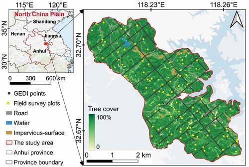
The study area is located in Mingguang County, Chuzhou City, Anhui Province, China (Figure 1), covering an area of nearly 1,650 ha with an average elevation of 32 m. The area belongs to the subtropical monsoon climate region with an annual average temperature of 15.4°C and precipitation between 700 and 1,400 mm. As part of the National Key Ecosystem Protection and Restoration Major Projects in China (NERPC), the masson pine forest vegetation in the study area was planted in the 1990s (Cui et al. 2021). Masson pine is an evergreen coniferous tree species having heights of 15 to 45 m. Branchlets usually grow twice per year. Each is colored yellowish brown, occasionally with a pale gray or bluish-green (glaucous) appearance. The tree species is fast-growing at in the beginning and growth gradually slows down in later years. Affected by climatic factors, understory vegetation is mainly composed of annual herbaceous vegetation and deciduous shrubs. The dominant species are Setaria viridis, Artemisia carvifolia, Dendranthema indicum, Duchesnea indica, Amaranthus spinosu, and Erigeron annuu. While masson pine is evergreen, the understory vegetation has no leaves during the non-growing season (October to April) but only during the growing season.

Figure 1. Location of the study area and surveyed plots superimposed on land use and cover information (Buchhorn et al. 2020; Nesha et al. 2021) for the measurements of the plant area index conducted in February and July 2020. The black dots indicate the GEDI footprints used in this study.

2.2 Field data collection

We conducted two field surveys covering the same plots (Figure 1) during the non-growing season (25 Feb 2020) and the growing season (15 Jul 2020) (Table 1). We sampled along a diagonal (Figure 2a) and we chose the sampling dates close to the Sentinel-2 satellite over-pass dates. In total, 86 plots each 10 × 10 m were randomly selected, being consistent with the pixel size of Sentinel-2 images (Figure 2b). In each plot, we used a LAI-2200C plant canopy analyzer (Li-Cor Biosciences, Lincoln, NE, USA) to measure the plant area index (PAI) (Rodríguez‐Ronderos et al. 2016). The PAI is the sum of leaf area index (LAI) and wood area index (WAI) (Kalacska et al. 2005; Sylvain and Leblanc 2001). We selected five positions of equal distance along the diagonal direction of each plot, and measured the PAI for all vegetative layers above the soil surface and at the height of the tree layer, defined as trees taller than 1.5 m (Figure 2b). The measured PAI for all-vegetative layers is a mixed signal from grasses, shrubs, and trees, whereas PAI for the tree layer only contains information from the coniferous forest canopy. Since the understory vegetation was not photosynthetically active during the non-growing season, only the tree layer was measured. We used the FV2200 software (Li-COR Biosciences) for field data post-processing. We also recorded GPS positions for the sampled sites and recorded basic vegetation information such as plant shape, leaf size, and moisture content. We implemented the same measurements for all vegetative layers and the tree layer for all plots during the growing season survey.

Figure 2. (a) Sampling positions (circles) along diagonals of a plot as part of the field measurements; (b) PAI observations; (c) two field photographs showing understory vegetation during the non-growing season and growing season.

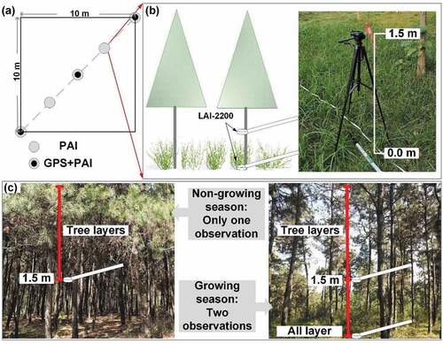
Table 1. Characteristics of data used in this study.

	Source	Level	Spatial resolution	Date acquired	Elements
Non-growing season	GEDI	L2B	25 m	5 December 2019, 15 January 2020	T00991, T03924
	Sentinel-2	L2A	10 m	28 December 2019	T024541
	Field data	-	10 m	28 February 2020	-
Growing season	GEDI	L2B	25 m	6 July 2020, 26 July 2020	T05260, T05500
	Sentinel-2	L2A	10 m	08 July 2020	T024549
	Field data	-	10 m	15 July 2020	-

2.3 GEDI LiDAR data

We downloaded GEDI LiDAR L2B data from the Land Processes Distributed Active Archive Center (LP DAAC) for January and July 2020, matching as closely as possible the dates of the field surveys and Sentinel-2 images (Table 1). The GEDI instrument records the amount of energy returned by various tree components at different heights above the ground and contains structural information, such as surface topography and metrics of canopy height, cover, and vertical profiles (Duncanson et al. 2020). Plant area volume density (PAVD) is a function of plant area per unit volume as a parameter obtained by the GEDI LiDAR instrument, which is often used to quantify the vertical structure of forests. PAI is defined as the one-sided area of plant material surface per unit ground surface area, which includes different constituents in the plant (e.g. stem, branches, and leaves). The two metrics are generated based on the directional gap probability profile derived from the wave-forms provided in the L1B products of GEDI LiDAR and locations of reflecting surfaces (Dubayah et al. 2020). Specifically, the canopy gap probability was firstly derived by the LiDAR waveform, and then the vegetation structure parameters were calculated using the cumulative laser energy return under the known canopy to ground reflectance ratio.

In our study, both the PAI and PAVD were extracted from 1,532 observations from GEDI L2B (Dubayah et al. 2020). GEDI has eight ground tracks, and the two metrics extracted from the four full-power beams relative to “coverage” beams were used (Silva et al. 2020). The sensitivity of a GEDI footprint indicates the maximum canopy cover that can be penetrated considering the signal-to-noise ratio of the waveform, and we thus excluded footprints with the sensitivity less than 0.9. After filtering out these invalid observations, 881 pairs of PAI and PAVD were used for further analysis.

2.4 Sentinel-2 data

Two tiles of Sentinel-2 Level 2A images were downloaded from the Copernicus Open Access (COA) Hub (scihub.copernicus.eu/), acquired on 28 December 2019 and 8 July 2020. The Sentinel-2 images were atmospherically corrected using the Sen2Cor plug-in provided by the ESA. The near-infrared (NIR) and short-wave infrared (SWIR) bands at 20 m spatial resolution were resampled to 10 m using the bicubic convolution interpolation method. In addition to these Sentinel-2 spectral bands, we calculated multiple vegetation indices that are widely used for classifying vegetation (Xi et al. 2021), canopy height (Li et al. 2020) and biomass (Chen et al. 2021). As a result, a total of 40 vegetation indices and 20 spectral band with a spatial resolution of 10 m were extracted. The details of the vegetation indices are displayed in Appendix A, Table A1.

3. Method

3.1 Selection of Sentinel-2 features

Advances in satellite technology offer a rich collection of spectral bands and associated vegetation indices that are often highly correlated. It is thus critical to reduce redundant features by assessing the variable collinearity that can improve the interpretability of the model and shorten data processing times (Erinjery, Singh, and Kent 2018; Grabska, Frantz, and Ostapowicz 2020). We conducted two steps to remove the redundant features: (1) We first removed candidate features with stronger collinearity (p < 0.05) by performing collinearity tests between all Sentinel-2 features (Table A2), (2) Recursive feature elimination (RFE) (Guyon and Barnhil S 2002) was then applied to identify the key features from 30 features comprising 10 bands and 20 metrics extracted from Sentinel-2. The key feature selection in RFE was conducted with a decision tree as the regression model and R-score stopping criteria. The selection of features is stopped when additional variables do not significantly (p < 0.05) improve the R-score.

3.2 Algorithms to map understory vegetation density

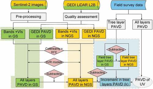
In this study, we conducted four main steps to quantify understory vegetation density. (1) the pre-processed GEDI data and Sentinel-2 images were divided into two groups of growing and non-growing season acquisitions in order to make use of the phenological difference to derive PAVD. (2) GEDI LiDAR data were used as dependent variables, and Sentinel-2-based features were used as independent variables for feature importance assessment and regression analysis. (3) We used the growing season PAVD subtracted by the non-growing season PAVD and the associated PAVD of increasing canopy to derive understory vegetation density. (4) The understory vegetation density was validated using field samples. The overall work-flow of PAVD mapping is presented in Figure 3.

Figure 3. Overall workflow of the understory vegetation estimation. The green and yellow shading indicates the estimation process of PAVD in the growing season and non-growing season respectively, while the blue shading involves the increment of PAVD in the forest canopy. GS: growing season, NGS: non-growing season, and UV: understory vegetation density.

3.2.1 Establishment of function between PAVD and PAI in GEDI LiDAR data

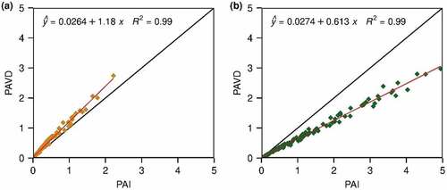
PAI is related to canopy foliage and crown structure, and has been widely used for assessing the structure and functions of forest ecosystems (Sylvain and Leblanc 2001; Tang et al. 2014). Accurate PAI values can be obtained from field observations, whereas from remotely sensed observations understory vegetation density is usually represented by PAVD indices, e.g. in studies based on LiDAR data (Campbell et al. 2018; Crespo-Peremarch et al. 2018). Based on the GEDI LiDAR data, we observed a strong correlation between PAI and PAVD for both the growing season and non-growing season (R² = 0.99, p < 0.01) (Figure 4). As a result, the field measured PAI has potential to characterize the understory vegetation density and will be converted to PAVD used as an independent data source to validate the satellite-derived understory vegetation density in this study.

Figure 4. Relationships between plant area index (PAI) and plant area volume density (PAVD) for (a) non-growing season; and (b) growing season.

3.2.2 Principle of understory vegetation density extraction

Understory vegetation is expected to predominantly contribute to the phenological differences in PAVD between the growing and non-growing season (see Section 2.2), and we thus used the growing season PAVD subtracted by the non-growing season PAVD to estimate understory vegetation density from GEDI LiDAR data. It should be noted that increment in woody foliage from non-growing season to growing season also contributes to the seasonal differences in PAVD. We thus used our field measured PAVD of the tree layers to calculate the increased PAVD by subtracting the averaged growing-season PAVD by the averaged non-growing-season PAVD using all plots. We applied this fixed PAVD increment to calibrate satellite derived PAVD. This approach is considered valid because the dominant tree species in this study area is masson pine characterized by the same stand age. Hence, we can approximately treat the seasonal increment of PAVD as a constant (Figure 5). Therefore, understory vegetation density (UV) can be calculated using the following equation:

Figure 5. Field measured PAVD of tree layers in the non-growing season and growing season. The green and yellow horizontal lines denote the average PAVD values of the tree layers for the growing season and non-growing season, respectively. PAVD were converted from PAI using the equations in Figure 4. The PAVD values from field survey are used to estimate k, which is a constant referring to the seasonal increment of PAVD required to compute understory vegetation density from PAVD of GEDI data. In this study, the k value was 0.39.

(1) $UV=PAV{D}_{GS}-PAV{D}_{NGS}-k$(1)

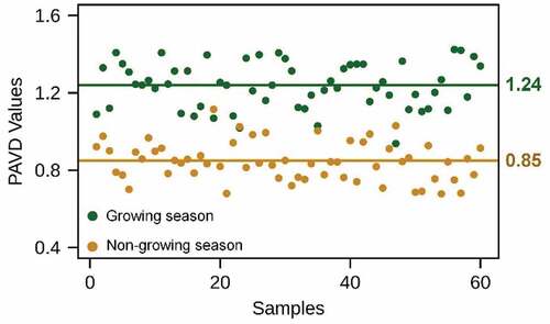
Where $PAV{D}_{GS}$ is the growing season PAVD, and $PAV{D}_{NGS}$ is the PAVD of non-growing season from GEDI LiDAR data. $k$ is a constant, which refers to the increment of PAVD in the forest canopy.

3.2.3 Mapping understory vegetation density

Given the limited number of training samples, we used a support vector regression (SVR) model to train the selected features from Sentinel-2 using 80% of the GEDI data observations. Multivariate SVR is a regression version of support vector machines that project the training dataset from a lower dimensional space into a higher dimensional space by using a kernel function, which is effective for the regression of complex, high-dimensional data providing multivariate, non-linear, and nonparametric regression. We used the radial basis function (RBF) in our study. Compared to other kernel functions, RBF compresses the training process and increases the calculation efficiency. Based on ten-fold cross-validation, the hyper-parameter sets as shown in Table 2 are tuned to obtain the best fit, including gamma, regularization parameter ($C$) and the kernel width ($\sigma$) for growing and non-growing season. The optimal models were run for the growing and non-growing season to derive PAVD maps covering the entire study area from Sentinel-2 imagery.

Table 2. Hyper-parameter setting of the SVR models in the growing season and non-growing season.

	Kernel	gamma	C	Epsilon
Growing season	rbf	1.6	120	0.1
Non-growing season	rbf	0.5	100	0.1

Note: “rbf” denotes radial basis function.

In addition, considering that the GEDI lidar beams have a 25 m footprint with a positional accuracy of 15 m (Coyle et al. 2015), we tested the GEDI LiDAR points with Sentinel pixels with pixel window-sizes of 2 × 2, 3 × 3, and 5 × 5 in the SVR model estimation. Our test results showed that applying the average values of four neighboring pixels (5 × 5) to match the GEDI LiDAR points produced the highest performance. As a result, we build training datasets and optimized SVR models to estimate vegetation density. Next, the understory vegetation density was calculated using the derived map and equation (1)(1) $UV=PAV{D}_{GS}-PAV{D}_{NGS}-k$(1) . k is converted from PAI using the linear regressions (see Figure 4).

3.3 Accuracy assessment

PAVD maps for the growing and non-growing seasons were validated using the remaining 20% of the GEDI-based PAVD samples. Additionally, the derived map of understory vegetation density was validated by independent field samples from the 86 plots. The coefficient of determination (R²), and the relative root mean square error (rRMSE) were used for the accuracy assessment.

4. Results

4.1 Sentinel-2 feature importance

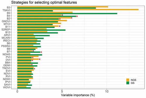
To find the optimal number of features, cross-validation was used with RFE to score different feature subsets and select the best scoring collection of features. In the growing season, we identified four spectral bands (B3, B5, B8, and B11) and seven vegetation indices (TSAVI, GNDVI, S2REP, ARVI, MCARI, NDI45, and PSSRA), which strongly explained the variations in PAVD (R score reaching 0.79) and from where additional variables did not increase the R score markedly (Figure 6a). In the non-growing season, a total of 12 variables were identified, namely B3, B5, B6, B8, B11, B12, TSAVI, GNDVI, MTCI, S2REP, PSSRA, and DVI, with an R score of 0.81 (Figure 6b). The detailed results of variable importance are displayed in Appendix A, Figure A1.

Figure 6. Feature contribution score and its standard deviation for (a) the growing season and (b) non-growing season. The vertical dashed red lines indicate the optimal number of features selected for the estimates of PAVD, corresponding to 11 features for the growing season and 12 for the non-growing season.

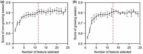
For Sentinel-2 spectral bands, red-edge, and NIR were closely related to PAVD for both the growing season and non-growing season. For VIs, the TSAVI, GNDVI, S2REP, ARVI, and NDI45 were identified as the most important metrics explaining the variations in PAVD during the growing season, while TSAVI, GNDVI, MTCI, S2REP, and PSSRA contributed the most to explained variation in PAVD for the non-growing season. The spectral band of B5 and the index of TSAVI were ranked the highest for the growing season and non-growing season, respectively.

4.2 Sentinel-2 derived PAVD estimation during the growing and non-growing season

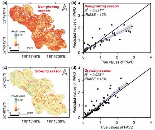
Based on GEDI LiDAR training data and the selected optimal features from Sentinel-2, PAVD was calculated using the SVR model for both the growing and non-growing season. The PAVD maps of the growing and non-growing season (Figure 7(a,c)), produced in a 10 m spatial resolution, reveal a considerable spatial heterogeneity of PAVD in the study area and notable differences in PAVD between growing and non-growing seasons. PAVD is generally lower in the non-growing season as compared to PAVD in the growing season, but some scattered areas show high PAVD, such as in the north-eastern and south-eastern part of the study area. Moreover, low PAVD values are observed along road and river courses during the growing season. Based on the independent GEDI samples, the accuracy of the PAVD maps for the growing and non-growing seasons are R² = 0.93(±0.01) and rRMSE = 15% (Figure 7b) and R² = 0.89(±0.03) and rRMSE = 13% (Figure 7d), respectively.

Figure 7. The PAVD 10-meter spatial resolution maps and accuracy for the non-growing season (a-b) and the growing season (c-d). ** denotes a significant relation at the 0.01 level and the shading indicates 95% confidence interval of the linear fitting.

4.3 Understory vegetation density mapping and validation

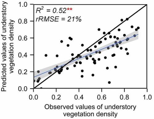
The understory vegetation density was derived based on equation (1)(1) $UV=PAV{D}_{GS}-PAV{D}_{NGS}-k$(1) (Section 3.2). From Figure 8a, the averaged understory vegetation density is 0.31 in the study area. Relatively high understory vegetation density is mainly observed in the northwest and central part of the study area, while a relatively low understory vegetation density is observed in the southern part. A small proportion (0.97%) of understory vegetation density values is marginally smaller than 0, mainly located in the southern and southeast of the study area. This can be attributed to the estimated error and is an inevitable consequence of using a regression-based approach, and such negative values can of course be reclassified into zero-values. We also show three different subsets of the predicted understory vegetation density and the corresponding Google Earth images for visual interpretation (Figure 8b-c). It clearly shows less understory vegetation density along built-up areas and roads (gray color), while there was a high understory vegetation density in densely forested areas. Compared with field data, our estimates of understory vegetation density show moderate correlations with R² = 0.52 and rRMSE = 21% (Figure 9). The highly significant relationship found (p < 0.01), however, clearly indicates this as a promising way forward to model understory vegetation density over large areas using GEDI LiDAR and Sentinel-2 data.

Figure 8. (a) Spatial distribution of modeled understory vegetation density with a histogram insert showing the distribution of the values, (b) three zoom-in illustrations of understory vegetation density, (c) corresponding Google Earth images.

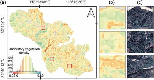
Figure 9. Validation of the understory vegetation density estimation using independent field-collected samples (n = 86). ** denotes a significant relation at the 0.01 level and the shading indicates 95% confidence interval of the linear fitting.

5. Discussion

5.1 Mapping understory vegetation density

We developed a new methodology to derive a continuous map of understory vegetation density in the Anhui Province, China using GEDI LiDAR and Sentinel-2. The correlation with field data was highly significant, yet not very high. This might partly be explained by the uncertainties of field observations due to small differences in the viewing angles and geolocation between field measurements and Sentinel-2 pixels (Hancock et al. 2017; Hill and Broughton 2009) as well as a general difference in the spatial scale of the footprint of observations between ground and satellite observations. A clear underestimation of high understory vegetation density is observed and vice versa for low values of understory vegetation density (Figure 8). This reflects the inability of the model to correctly predict the extreme values measured in the field, as these tends to be evened out from the use of satellite data for the above-mentioned reasons. The Airborne LiDAR-based studies of understory vegetation reports a similar range of R² values (Campbell et al. 2018; Hill and Broughton 2009), and our results underlines a solid potential of using freely available LiDAR and optical data in combination to estimate continuous understory vegetation density. The approach is expected to be adoptable over large areas given some preconditions are met (see below), which would improve the estimation of total forest carbon storage and dynamics to improve our understanding of terrestrial ecosystem processes (Duncanson et al. 2020).

5.2 Prospects of GEDI LiDAR and Sentinel-2 data

Previous studies have shown that a waveform LiDAR system with ~25 m horizontal resolution and ~1 m vertical accuracy can support accurate measurement of vertical canopy structure (± 10%) in presence of moderate slopes of terrain (Potapov et al. 2021). These requirements fit well into the current design of GEDI for estimating canopy cover (Kokalj and Mast 2021), LAI (Estévez et al. 2020) and foliage height diversity (Tang et al. 2019). We thus used the directional gap probability profile which is derived from the waveforms provided in the L1B product and locations of reflecting surfaces to extract vegetation density from each GEDI waveform used to generate the structural metrics of PAI and PAVD. The established relationship between PAVD and the optical spectral bands of Sentinel-2 are primarily dependent on the strong capacity of the multiple optical spectral bands of Sentinel-2 to capture the structural and functional characteristics of vegetation. In particular, the red-edge bands are highly related to vegetation leaf properties, such as leaf area index, biomass, and structural carbohydrates (Martin-Gallego et al., 2020), while NIR and SWIR bands are sensitive to the changes of water content, lignin, starch, and nitrogen (Fassnacht et al., 2016). These optical spectral bands have been successfully used to estimate forest biomass (Chen et al. 2021), canopy density (Qi and Dubayah 2016) and forest height (Henrik J and Roland 2016) in recent studies as well. We also rely on the close linear relationship between PAI and PAVD that enables the field measured PAI conversion to PAVD, which provides the independent samples to validate the resultant map of understory vegetation density.

5.3 Limitations of understory vegetation density mapping

There are several issues that may limit the applicability of our approach for mapping vegetation understory density. Firstly, in relation to the field survey, the masson pine in our study area was planted at the same time resulting in all trees having almost same height and crown sizes, thereby showing strong homogeneity of the forest canopy. This makes it possible to apply a constant value over the study areas to estimate the increment in the PAVD resulting from seasonal variations in the forest canopy between the growing season and non-growing season. Our approach applies to coniferous forest, however, other types of forests could have different responses resulting from species- or community-level differences in plant physiology, leading to variable seasonal increment in the PAVD for the forest canopy between non-growing season and growing season. In such case, the method developed in our study should be used with caution given the spatial variations of PAVD increment, and more research is needed to further advance the feasibility of the method developed here. Secondly, current GEDI LiDAR data using the laser energy distribution (near-infrared wavelengths) could have limitations when forest canopies are dense such as in the case of rainforest (Bauer, Knapp, and Fischer 2021). Under such conditions, the complementary use of L-band SAR data may advance the capacity for estimating understory vegetation density (Vittucci et al. 2021). Moreover, other machine learning approaches used for upscaling such as random forest, and extreme gradient boosting, should be considered to test if consistent results are obtained when estimating understory vegetation density. Thirdly, there are some inevitable systematic errors associated with the estimation process. For example, the residual geo-location error of the GEDI data (25 m per footprint) affects the calibration of the Sentinel-based (10 m per pixel) model and validation at foot-print level. The different acquisition time of GEDI LiDAR data, Sentinel-2 images may bring in uncertainty on the estimations of the related variables, however, the maximum 11-day time interval between field observations and remote sensing data acquisition ensured that vegetation structure did not change significantly between the acquisition of the different types of data. In the non-growing season, the acquisition dates of the three data sources were more distant in time, but as the vegetation structure remains unchanged during this period (evergreen coniferous forest without understory vegetation) this has no impact on the design of the analysis. Additionally, the bare soil background including the shading caused by tree canopy and topography could cause biases in the reflectance values of the Sentinel-2 data.

6. Conclusion

Based on the differences in vegetation phenology, our study proposes an effective and practical approach to quantify understory vegetation density using GEDI and Sentinel-2 data in a coniferous forest setting in China, characterized by a subtropical monsoon climate. We produce a map of understory vegetation density that performed well when compared against independent field samples (R² = 0.52 and rRMSE = 21%, p < 0.01). In particular, our approach has shown a promising potential for mapping understory vegetation density for a temperate conifer ecosystem (e.g. Carpathian, Da Hing-gan-Dzhagdy, and Siberia) with sparse trees, favoring the laser light penetrate forest canopy to detect understory vegetation. Such large-scale understory vegetation mapping provides a way toward quantifying missing information on the understory vegetation stratum for a complete assessment of forest biomass resources. However, the robustness and accuracy of estimations in different forest ecosystem types should be further tested, taking into consideration different characteristics of forest types, such as boreal and temperate forest, broadleaf and needles forest, and forests of various densities. In summary, with the combination of GEDI LiDAR data and Sentinel-2 imagery our study succeeded in mapping spatially continuous understory vegetation density, which holds promises for improving the estimation of terrestrial carbon storage and providing the basis for a better understanding of various forest ecosystem processes across larger areas.

Acknowledgements

This work was supported by National Natural Science Foundation of China (42101321), China Postdoctoral Science Foundation (2021M701653), W.M.Z. and M.B. are supported by ERC project TOFDRY (grant number: 947757). W.M.Z. also acknowledge funding from the National Natural Science Foundation of China (grant number: 42001349). Y.X. are supported by the China Scholarship Council (202106190083).

Disclosure statement

No potential conflict of interest was reported by the author(s).

Data availability statement

The data that support the findings of this study are available from the corresponding author, Q.T., upon reasonable request.

Correction Statement

This article has been corrected with minor changes. These changes do not impact the academic content of the article.

Additional information

Funding

This work was supported by the China Postdoctoral Science Foundation [2021M701653]; China Scholarship Council [202106190083]; National Natural Science Foundation of China [42001349]; National Natural Science Foundation of China [42101321].

Appendix A

Figure A1. Relative importance of each variable in estimating understory vegetation density. × means that the variables are removed by using collinearity.

Appendix B

Table A1. Vegetation indices applied and its characteristics.

Sensitive with	Vegetation indices	Equation	References
Soil background	Soil Adjusted Vegetation Index (SAVI)	1.5(B8-B4)/(B8+ B4 + 0.5)	Huete (1988)
	Transformed Soil Adjusted Vegetation Index (TSAVI)	s(B8-s*B4-a))/(a*B8+ B4-a*s + X*(1+ s^2)	Baret et al. (1989)
Atmospheric variations	Weighted Difference Vegetation Index (WDVI)	B8-g*B4	Clevers (1988)
	Perpendicular Vegetation Index (PVI)	Sin(a)*B8-cos(a)*B4	Richardson and Wiegand (1977)
	Global Environmental Monitoring Index (GEMI)	n(1–0.25 n)-(B4-0.125)/(1-B4)	Pinty and Verstraete (1991)
Water content of vegetation	Normalized Difference Water Index (NDWI)	(B8-B11)/(B8+ B11)	Gao (1996)
Low vegetation	Normalized Difference Vegetation Index (NDVI)	(B8-B4)/(B8+ B4)	Tucker (1979)
	Infrared Percentage Vegetation Index (IPVI)	B8/(B8+ B4)	Crippen (1990)
	Transformed Normalized Difference Vegetation Index (TNDVI)	Sqrt((B8-B4)/(B8+ B4)+0.5)	Sensema et al. (1996)
High vegetation	Ratio Vegetation Index (RVI)	B8/B4	Major, Baret, and Guyot (2007)
	Normalized Difference Index (NDI45)	(B5 – B4)/(B5 + B4)	Delegido et al. (2011)
	Enhanced Vegetation Index (EVI)	2.5((B8-B4)/(L+ B8+ CB4))	Matsushita et al. (2007)
Chlorophyll content	Green Normalized Difference Vegetation index (GNDVI)	(B7-B3)/(B7+ B3)	Lopes and Reynolds (2012)
	Normalized difference red-edge index (NDRE)	(B8-B6)/(B8+ B6)	Clevers and Gitelson (2013)
	Inverted Red-Edge Chlorophyll Index (IRECI)	(B7-B4)/(B5/B6)	Guyot and Baret (1988)
	MERIS Terrestrial Chlorophyll Index (MTCI)	(B6-B5)/(B5-B4)	Dash and Curran (2007)
	Modified Chlorophyll Absorption Ratio Index (MCARI)	((B5-B4)-0.2(B5-B3))/(B5/B4)	Yang et al. (2006)
Nitrogen content	Sentinel-2 Red-Edge Position (S2REP)	705 + 35*((B4 + B7)/2 – B5)/(B6 – B5)	Herrmann et al. (2010)
Canopy density	Pigment Specific Simple Ratio (PSSRA)	B7/B4	Blackburn (1999)
	Difference Vegetation Index (DVI)	B8-B4	Major, Baret, and Guyot (2007)

Appendix C

Table A2. The collinearity result of predictor variables derived from Sentinel-2 images. R-value is the correlation between the variable and PAVD **: Significant correlation (p < 0.01), *: Significant correlation (p < 0.05). Predictors are the ones chosen for the recursive feature elimination.

Related variables	Non-growing season			Growing Season
	R PAVD	Collinear with	Predictors	R PAVD	Collinear with	Predictors
B2	0.23**	B3, B4, GNDVI	No	0.28**	B3, B4	No
B3	0.27**	B2, B4, B5	Yes	0.34**	B2, B4, B5, NDVI	Yes
B4	0.25**	B2, B3, B5, B11, B12	No	0.30**	B5, NDVI	No
B5	0.28**	B2, B3, B4, B11	Yes	0.32**	B2, B4, B12	Yes
B6	0.11*	B7, B8, B8A	Yes	0.21**	B7, B8, B8A	Yes
B7	0.09*	B6, B8, B8A, GEMI	No	0.12*	B6, B8, B8A	No
B8	0.12*	B6, B7, B8A	Yes	0.17**	B7, B8A, GEMI	Yes
B8A	0.11*	B6, B7, B8	Yes	0.15*	GEMI, B8	Yes
B11	0.24**	B12	Yes	0.18**	/	Yes
B12	0.23**	B11	No	0.24**	B4	Yes
SAVI	0.06	NDVI, PVI	Yes	0.07*	/	Yes
TSAVI	0.16**	/	Yes	0.08*	/	Yes
WDVI	0.09*	TNDVI, PVI, ARVI, IRECI	Yes	0.10*	PVI, GEMI	Yes
PVI	0.06*	WDVI, GEMI	Yes	−0.02	WDVI, GEMI, DVI	No
GEMI	−0.00	IRECI, B6, B7, B8, B8A	No	−0.07*	PVI, WDVI	Yes
NDWI	0.14**	/	Yes	0.15**	/	Yes
NDVI	0.18**	B2, B3, B4, B5, DVI, RVI, PVI, IPVI, TNDVI	Yes	0.24**	B2, B3, B4, B5, DVI, RVI, IPVI, WDVI, TNDVI	Yes
IPVI	0.18**	RVI, NDVI, TNDVI, SAVI, GNDVI	Yes	0.24**	RVI, NDVI, TNDVI, GNDVI, ARVI	Yes
TNDVI	0.18**	NDVI, GNDVI, ARVI, NDI45, GEMI	Yes	0.23**	NDVI, GNDVI, ARVI	No
RVI	0.17**	NDVI, IPVI, WDVI, TNDVI, ARVI	Yes	0.25**	NDVI, DVI, IPVI, TDVI	Yes
NDI45	0.15**	PSSRA	Yes	0.20**	/	Yes
EVI	0.34**	RVI, NDVI, SAVI, ARVI, PSSRA	Yes	0.32**	RVI, NDVI, SAVI, ARVI, PSSRA	Yes
GNDVI	0.23**	NDVI, IPVI, TNDVI, ARVI, RVI, DVI	Yes	0.29**	NDVI, TNDVI, ARVI, RVI, DVI	Yes
NDRE	0.13**	/	Yes	0.12*	/	Yes
IRECI	0.11*	/	Yes	0.17**	/	Yes
MTCI	0.10*	/	Yes	0.13*	/	Yes
MCARI	0.07*	/	Yes	0.08*	/	Yes
S2REP	0.05*	/	Yes	0.23**	/	Yes
PSSRA	0.19**	EVI, NDVI, RVI, TNDVI, WDVI	Yes	0.29**	NDVI, RVI, IPVI, TNDVI, ARVI	Yes
DVI	0.03	B8, NDVI, SAVI	No	−0.02	PVI, WDVI, GEMI	No

References

- Baret F., G. Guyot and D. Major. 1989. “Crop biomass evaluation using radiometric measurements.“ Photogrammetria 43 (5): 241–256. doi:10.1016/0031-8663(89)90001-X
- Bauer, L., N. Knapp, and R. Fischer. 2021. “Mapping Amazon Forest Productivity by Fusing GEDI Lidar Waveforms with an Individual-Based Forest Model.” Remote Sensing 13 (22): 4540. doi:10.3390/rs13224540.
- Bihamta Toosi, N., A. R. Soffianian, S. Fakheran, S. Pourmanafi, C. Ginzler, and T. Waser, L. 2020. “Land Cover Classification in Mangrove Ecosystems Based on VHR Satellite Data and Machine learning—an Upscaling Approach.” Remote Sensing 12 (17): 2684. doi:10.3390/rs12172684.
- Blackburn, G. A. 1999. “Relationships between Spectral Reflectance and Pigment Concentrations in Stacks of Deciduous Broadleaves.” Remote Sensing of Environment 70 (2): 224–237. doi:10.1016/S0034-4257(99)00048-6.
- Buchhorn M., M. Lesiv, N. Tsendbazar, M. Herold, L. Bertels and B. Smets. 2020. “Copernicus Global Land Cover Layers—Collection 2.“ Remote Sensing 12 (6): 1044. doi:10.3390/rs12061044
- Campbell, M. J., P. E. Dennison, A. T. Hudak, L. M. Parham, and B. W. Butler. 2018. “Quantifying Understory Vegetation Density Using small-footprint Airborne Lidar.” Remote Sensing of Environment 215: 330–342. doi:10.1016/j.rse.2018.06.023.
- Chen, L., C. Ren, B. Zhang, Z. Wang, M. Liu, W. Man, and J. Liu. 2021. “Improved Estimation of Forest Stand Volume by the Integration of GEDI LiDAR Data and multi-sensor Imagery in the Changbai Mountains Mixed Forests Ecoregion (CMMFE), Northeast China.” International Journal of Applied Earth Observation and Geoinformation 100: 102326. doi:10.1016/j.jag.2021.102326.
- Clevers J. 1988. “The derivation of a simplified reflectance model for the estimation of leaf area index.“ Remote Sensing of Environment 25 (1): 53–69. doi:10.1016/0034-4257(88)90041-7
- Clevers, J. G. P. W., and A. A. Gitelson. 2013. “Remote Estimation of Crop and Grass Chlorophyll and Nitrogen Content Using red-edge Bands on Sentinel-2 and −3.” International Journal of Applied Earth Observation and Geoinformation 23: 344–351. doi:10.1016/j.jag.2012.10.008.
- Coyle, D. B., P. R. Stysley, D. Poulios, G. B. Clarke, and R. B. Kay. 2015. “Laser Transmitter Development for NASA’s Global Ecosystem Dynamics Investigation (GEDI) Lidar.” In Lidar Remote Sensing for Environmental Monitoring XV, 19–25. SPEI. Digital Library: SPIE. https://doi.org/10.1117/12.2191569
- Crespo-Peremarch, P., P. Tompalski, N. C. Coops, and L. Á. Ruiz. 2018. “Characterizing Understory Vegetation in Mediterranean Forests Using full-waveform Airborne Laser Scanning Data.” Remote Sensing of Environment 217: 400–413. doi:10.1016/j.rse.2018.08.033.
- Crippen, R. E. 1990. “Calculating the Vegetation Index Faster.” Remote Sensing of Environment 34: 71–73. doi:10.1016/0034-4257(90)90085-Z.
- Cui, W., J. Liu, J. Jia, and P. Wang. 2021. “Terrestrial Ecological Restoration in China: Identifying Advances and Gaps.” Environmental Sciences Europe 33 (1): 1–14. doi:10.1186/s12302-021-00563-2.
- Dash, J., and P. J. Curran. 2007. “Evaluation of the MERIS Terrestrial Chlorophyll Index (MTCI).” Advances in Space Research 39 (1): 100–104. doi:10.1016/j.asr.2006.02.034.
- Delegido J., J. Verrelst, L. Alonso and J. Moreno. 2011. “Evaluation of Sentinel-2 Red-Edge Bands for Empirical Estimation of Green LAI and Chlorophyll Content.“ Sensors 11 (7): 7063–7081. doi:10.3390/s110707063
- Dubayah, R., J. B. Blair, S. Goetz, L. Fatoyinbo, M. Hansen, S. Healey, M. Hofton, et al. 2020. “The Global Ecosystem Dynamics Investigation: High-resolution Laser Ranging of the Earth’s Forests and Topography.” Science of Remote Sensing 1: 100002. doi:10.1016/j.srs.2020.100002.
- Duncanson, L., A. Neuenschwander, S. Hancock, N. Thomas, T. Fatoyinbo, M. Simard, C. A. Silva, et al. 2020. “Biomass Estimation from Simulated GEDI, ICESat-2 and NISAR across Environmental Gradients in Sonoma County, California.” Remote Sensing of Environment 242: 111779. doi:10.1016/j.rse.2020.111779.
- Echiverri, L., and S. E. Macdonald. 2019. “Utilizing a Topographic Moisture Index to Characterize Understory Vegetation Patterns in the Boreal Forest.” Forest Ecology and Management 447: 35–52. doi:10.1016/j.foreco.2019.05.054.
- Erinjery, J. J., M. Singh, and R. Kent. 2018. “Mapping and Assessment of Vegetation Types in the Tropical Rainforests of the Western Ghats Using Multispectral Sentinel-2 and SAR Sentinel-1 Satellite Imagery.” Remote Sensing of Environment 216: 345–354. doi:10.1016/j.rse.2018.07.006.
- Estévez, J., J. Vicent, J. P. Rivera-Caicedo, P. Morcillo-Pallarés, F. Vuolo, N. Sabater, G. Camps-Valls, J. Moreno, and J. Verrelst. 2020. “Gaussian Processes Retrieval of LAI from Sentinel-2 top-of-atmosphere Radiance Data.” ISPRS Journal of Photogrammetry and Remote Sensing 167: 289–304. doi:10.1016/j.isprsjprs.2020.07.004.
- Fassnacht F. E., H. Latifi, K. Stereńczak, A. Modzelewska, M. Lefsky, L. T. Waser, C. Straub and A. Ghosh. 2016. “Review of studies on tree species classification from remotely sensed data.“ Remote Sensing of Environment 186: 64–87. doi:10.1016/j.rse.2016.08.013
- Gao, G., S.Ting-Toomey, and W. B. Gudykunst. 1996. “Chinese communication processes.“ In M. H. Bond (Ed.), The handbook of Chinese psychology (pp. 280–293). Oxford University Press.
- Grabska, E., D. Frantz, and K. Ostapowicz. 2020. “Evaluation of Machine Learning Algorithms for Forest Stand Species Mapping Using Sentinel-2 Imagery and Environmental Data in the Polish Carpathians.” Remote Sensing of Environment 251: 112103. doi:10.1016/j.rse.2020.112103.
- Guyon, I., and W. J. Barnhil S. 2002. “Gene Selection for Cancer Classification Using Support Vector Machines.” Machine Learning 46 (1): 389–422. https://doi.org/10.1023/A:1012487302797
- Guyot, G., and F. Baret. 1988. “Utilisation de la haute resolution spectrale pour suivre l'etat des couverts vegetaux.“ Spectral Signatures of Objects in Remote Sensing 287: 279.
- Hancock, S., K. Anderson, M. Disney, and K. J. Gaston. 2017. “Measurement of fine-spatial-resolution 3D Vegetation Structure with Airborne Waveform Lidar: Calibration and Validation with Voxelised Terrestrial Lidar.” Remote Sensing of Environment 188: 37–50. doi:10.1016/j.rse.2016.10.041.
- Herrmann, I., A. Pimstein, A. Karnieli, Y. Cohen, V. Alchanatis, and D. J. Bonfil, 2010. “Assessment of Leaf Area Index by the red-edge Inflection Point Derived from VENμS Bands.” InProceedings of the ESA hyperspectral workshop, Frascati, Italy 2010 March (Vol. 683, pp. 1–7).
- Hill R., and R. Broughton. 2009.“Mapping the understorey of deciduous woodland from leaf-on and leaf-off airborne LiDAR data: A case study in lowland Britain“ ISPRS Journal of Photogrammetry and Remote Sensing 64 (2): 223–233. doi:10.1016/j.isprsjprs.2008.12.004
- Huang, H., C. Liu, X. Wang, X. Zhou, and P. Gong. 2019. “Integration of multi-resource Remotely Sensed Data and Allometric Models for Forest Aboveground Biomass Estimation in China.” Remote Sensing of Environment 221: 225–234. doi:10.1016/j.rse.2018.11.017.
- Huete, A. R. 1988. “A Soil-Adjusted Vegetation Index (SAVI).” Remote Sensing of Environment 25 (3): 295–309. doi:10.1016/0034-4257(88)90106-X.
- Kalacska, M. E., G. A. Sánchez‐Azofeifa, J. C. Calvo‐Alvarado, B. Rivard, and M. Quesada. 2005. “Effects of Season and Successional Stage on Leaf Area Index and Spectral Vegetation Indices in Three Mesoamerican Tropical Dry Forests 1.” Biotropica: The Journal of Biology and Conservation 37 (4): 486–496. https://doi.org/10.1111/j.1744-7429.2005.00067.x
- Kokalj, Ž., and J. Mast. 2021. “Space Lidar for Archaeology? Reanalyzing GEDI Data for Detection of Ancient Maya Buildings.” Journal of Archaeological Science: Reports 36: 102811. https://doi.org/10.1016/j.jasrep.2021.102811
- Lee, Y. S., S. Lee, W. K. Baek, H. S. Jung, S. H. Park, and M. J. Lee. 2020. “Mapping Forest Vertical Structure in Jeju Island from Optical and Radar Satellite Images Using Artificial Neural Network.” Remote Sensing 12 (5): 797. https://doi.org/10.3390/rs12050797
- Li, W., Z. Niu, R. Shang, Y. Qin, L. Wang, and H. Chen. 2020. “High-resolution Mapping of Forest Canopy Height Using Machine Learning by Coupling ICESat-2 LiDAR with Sentinel-1, Sentinel-2 and Landsat-8 Data.” International Journal of Applied Earth Observation and Geoinformation 92: 102163. doi:10.1016/j.jag.2020.102163.
- Lopes, M. S., and M. P. Reynolds. 2012. “Stay-green in Spring Wheat Can Be Determined by Spectral Reflectance Measurements (Normalized Difference Vegetation Index) Independently from Phenology.” Journal of Experimental Botany 63 (10): 3789–3798. doi:10.1093/jxb/ers071.
- Major, D. J., F. Baret, and G. Guyot. 2007. “A Ratio Vegetation Index Adjusted for Soil Brightness.” International Journal of Remote Sensing 11: 727–740. https://doi.org/10.1080/01431169008955053
- Martin-Gallego P., P. Aplin, C. Marston, A. Altamirano and A. Pauchard. 2020. “Detecting and modelling alien tree presence using Sentinel-2 satellite imagery in Chile’s temperate forests“ Forest Ecology and Management 474: 118353. doi:10.1016/j.foreco.2020.118353
- Martinuzzi, S., L. A. Vierling, W. A. Gould, M. J. Falkowski, J. S. Evans, A. T. Hudak, and K. T. Vierling. 2009. “Mapping Snags and Understory Shrubs for a LiDAR-based Assessment of Wildlife Habitat Suitability.” Remote Sensing of Environment 113 (12): 2533–2546. doi:10.1016/j.rse.2009.07.002.
- Matsushita, B., W. Yang, J. Chen, Y. Onda, and G. J. S. Qiu. 2007. “Sensitivity of the Enhanced Vegetation Index (EVI) and Normalized Difference Vegetation Index (NDVI) to Topographic Effects: A Case Study in high-density Cypress Forest.” Sensors 7 (11): 2636–2651. doi:10.3390/s7112636.
- Nesha M. K., M. Herold, V. De Sy, A. E. Duchelle, C. Martius, A. Branthomme, M. Garzuglia, O. Jonsson and A. Pekkarinen. 2021.“An assessment of data sources, data quality and changes in national forest monitoring capacities in the Global Forest Resources Assessment 2005–2020.“Environmental Research Letters 16 (5): 054029. doi:10.1088/1748-9326/abd81b
- Persson H. J. and R. Perko. 2016. “Assessment of boreal forest height from WorldView-2 satellite stereo images.“ Remote Sensing Letters 7 (12): 1150–1159. doi:10.1080/2150704X.2016.1219424
- Pinty B. and M. M. Verstraete. 1991. “Extracting information on surface properties from bidirectional reflectance measurements.“ Journal of Geophysical Research: Atmosphere 96 (D2): 2865. doi:10.1029/90JD02239
- Potapov, P., X. Li, A. Hernandez-Serna, A. Tyukavina, M. C. Hansen, A. Kommareddy, A. Pickens, et al. 2021. “Mapping Global Forest Canopy Height through Integration of GEDI and Landsat Data.” Remote sensing of Environment 253: 112165. doi:10.1016/j.rse.2020.112165.
- Qi, W., and R. O. Dubayah. 2016. “Combining Tandem-X InSAR and Simulated GEDI Lidar Observations for Forest Structure Mapping.” Remote Sensing of Environment 187: 253–266. doi:10.1016/j.rse.2016.10.018.
- Richardson, A. J., and C. L. Wiegand 1977. ”Distinguishing vegetation from soil background information.” Photogrammetric engineering and remote sensing 43 (12): 1541–1552.
- Rodríguez‐Ronderos, M. E., G. Bohrer, A. Sanchez‐Azofeifa, J. S. Powers, and S. A. Schnitzer. 2016. “Contribution of Lianas to Plant Area Index and Canopy Structure in a Panamanian Forest.” Ecology 97 (12): 3271–3277. doi:10.1002/ecy.1597.
- Senseman G. M., C. F. Bagley and S. A. Tweddale. 1996. “Correlation of rangeland cover measures to satellite‐imagery‐derived vegetation indices.“ Geocarto International 11 (3): 29–38. doi:10.1080/10106049609354546
- Shen, W., M. Li, C. Huang, X. Tao, and A. Wei. 2018. “Annual Forest Aboveground Biomass Changes Mapped Using ICESat/GLAS Measurements, Historical Inventory Data, and time-series Optical and Radar Imagery for Guangdong Province, China.” Agricultural and Forest Meteorology 259: 23–38. doi:10.1016/j.agrformet.2018.04.005.
- Silva, C., C. Hamamura, R. Valbuena, S. Hancock, A. Cardil, E. Broadbent, D. Almeida, C. Silva-Junior, and C. Klauberg, 2020. “rGEDI: An R Package for NASA’s Global Ecosystem Dynamics Investigation (GEDI) Data Visualizing and Processing Version 0.1.8.” on October. 22 2020, available at 22 October 2020: https://CRAN.R-project.org/package=rGEDI
- Stysley, P. R., D. B. Coyle, R. B. Kay, R. Frederickson, D. Poulios, K. Cory, and G. Clarke. 2015. “Long Term Performance of the High Output Maximum Efficiency Resonator (HOMER) Laser for NASA׳s Global Ecosystem Dynamics Investigation (GEDI) Lidar.” Optics & Laser Technology 68: 67–72. doi:10.1016/j.optlastec.2014.11.001.
- Sylvain, G., and J. M. C. Leblanc. 2001. “A Practical Scheme for Correcting Multiple Scattering Effects on Optical LAI Measurements.” Agricultural and Forest Meteorology 110 (2): 125–139. doi:10.1016/S0168-1923(01)00284-2.
- Tang, H., J. Armston, S. Hancock, S. Marselis, S. Goetz, and R. Dubayah. 2019. “Characterizing Global Forest Canopy Cover Distribution Using Spaceborne Lidar.” Remote Sensing of Environment 231: 111262. doi:10.1016/j.rse.2019.111262.
- Tang, H., M. Brolly, F. Zhao, A. H. Strahler, C. L. Schaaf, S. Ganguly, G. Zhang, and R. Dubayah. 2014. “Deriving and Validating Leaf Area Index (LAI) at Multiple Spatial Scales through Lidar Remote Sensing: A Case Study in Sierra National Forest, CA.” Remote Sensing of Environment 143: 131–141. doi:10.1016/j.rse.2013.12.007.
- Tuanmu, M. N., A. Viña, S. Bearer, W. Xu, Z. Ouyang, H. Zhang, and J. Liu. 2010. “Mapping Understory Vegetation Using Phenological Characteristics Derived from Remotely Sensed Data.” Remote Sensing of Environment 114 (8): 1833–1844. https://doi.org/10.1016/j.rse.2010.03.008
- Tucker, C. J. 1979. “Red and Photographic Infrared Linear Combinations for Monitoring Vegetation.” Remote Sensing of Environment 8: 127–150. doi:10.1016/0034-4257(79)90013-0.
- Vittucci, C., L. Guerriero, P. Ferrazzoli, P. Richaume, and Y. H. Kerr. 2021. “SMOS L-VOD Retrieved by Level 2 Algorithm and Its Correlation with GEDI LIDAR Products.” IEEE Journal of Selected Topics in Applied Earth Observations and Remote Sensing 14: 11870–11878. doi:10.1109/JSTARS.2021.3128022.
- Wang, D., B. Wan, J. Liu, Y. Su, Q. Guo, P. Qiu, and X. J. Wu. 2020. “Estimating Aboveground Biomass of the Mangrove Forests on Northeast Hainan Island in China Using an Upscaling Method from Field Plots, UAV-LiDAR Data and Sentinel-2 Imagery.” International Journal of Applied Earth Observation and Geoinformation 85: 101986. doi:10.1016/j.jag.2019.101986.
- Wing, B. M., M. W. Ritchie, K. Boston, W. B. Cohen, A. Gitelman, and M. J. Olsen. 2012. “Prediction of Understory Vegetation Cover with Airborne Lidar in an Interior Ponderosa Pine Forest.” Remote Sensing of Environment 124: 730–741. doi:10.1016/j.rse.2012.06.024.
- Xi, Y., C. Ren, Q. Tian, Y. Ren, X. Dong, and Z. Zhang. 2021. “Exploitation of Time Series Sentinel-2 Data and Different Machine Learning Algorithms for Detailed Tree Species Classification.” IEEE Journal of Selected Topics in Applied Earth Observations and Remote Sensing 14: 7589–7603. doi:10.1109/JSTARS.2021.3098817.
- Xu, T., Z. Guo, S. Liu, X. He, Y. Meng, Z. Xu, and L. Song. 2018. “Evaluating Different Machine Learning Methods for Upscaling Evapotranspiration from Flux Towers to the Regional Scale.” Journal of Geophysical Research: Atmospheres 123 (16): 8674–8690. doi:10.1029/2018JD028447.
- Yang, X. H., J. F. Huang, F. M. Wang, X. Z. Wang, Q. X. Yi, and Y. Wang. 2006. “A Modified Chlorophyll Absorption Continuum Index for Chlorophyll Estimation.” Journal of Zhejiang University-SCIENCE A 7 (12): 2002–2006. https://doi.org/10.1631/jzus.2006.A2002
- Zhang, W., M. Brandt, Q. Wang, A. V. Prishchepov, C. J. Tucker, Y. Li, H. Lyu, and R. Fensholt. 2019. “From Woody Cover to Woody Canopies: How Sentinel-1 and Sentinel-2 Data Advance the Mapping of Woody Plants in Savannas.” Remote Sensing of Environment 234: 111465. doi:10.1016/j.rse.2019.111465.
- Zheng, G., and L. M. Moskal. 2009. “Retrieving Leaf Area Index (LAI) Using Remote Sensing: Theories, Methods, and Sensors.” Sensors (Basel) 9 (4): 2719–2745. https://doi.org/10.3390/s90402719