A framework for fine classification of urban wetlands based on random forest and knowledge rules: taking the wetland cities of Haikou and Yinchuan as examples

ABSTRACT

Urban wetlands play an important role in sustainable urban development. A wetland city recognized by the Ramsar Convention is a city with a remarkable ecological performance of urban wetlands and can provide an example for urban wetland protection. Therefore identifying the detailed characteristics of wetlands is of great value to the conservation of urban wetlands. However, there is no detailed wetland type extraction for wetland cities using multisource remote sensing data. This paper proposes a framework for fine- urban wetland extraction with multisource and multiperiod remote sensing data, which mainly includes Sentinel 1/2 and Landsat 8 data, and obtains the detailed wetland type data containing 14 wetland categories at a 10-m resolution. The classification methods of random forests were used to extract land cover types, and knowledge rules were used to classify detailed wetland types. The wetland cities, Yinchuan, and Haikou, located in southern and northern China, respectively, were chosen as case studies. The results indicate that the overall accuracy and wetland accuracy of the two cities in 2015 and 2020 were greater than 88% and 87%, respectively. The detailed wetland mapping results were more accurate and had a high resolution, and wetland categories were more diverse compared with other wetland-related products. According to the classification results, the wetland area in Haikou was 326.86 km² (13.43%) in 2015 and 308.58 km² (12.66%) in 2020. The wetland area in Yinchuan was 80.39 km² (4.46%) in 2015 and 74.15 km² (4.12%) in 2020. The fine urban wetland classification framework we propose and the detailed wetland results could serve for the creation of wetland cities and support the protection and rational use of urban wetlands.

KEYWORDS:

• Wetland city
• fine classification
• detailed urban wetland types
• multisource remote sensing

1. Introduction

With the development of cities, the relationship between wetlands and cities has been focus of attention. The wetland city concept recognized by the Ramsar Convention was developed with the idea that the relationship between wetlands and cities has gradually become a hot issue. The Wetland City Accreditation scheme also introduced by the Ramsar Convention may increase public awareness of wetlands and promote the conservation and wise use of urban wetlands (www.ramsar.org/activity/wetland-city-accreditation). Forty-three cities around the world have obtained the Wetland City Certificate (www.ramsar.org/activity/wetland-city-accreditation), which represents the city’s ecological achievements and a high-level and important honor in the world in terms of urban wetland ecological protection. Therefore, it is important to recognize the wetlands in these cities to protect them and foster the rational use of the wetland resources of the city.

Recognizing the detailed wetland characteristics and monitoring the wetland environment in real time for a wetland city are of great significance for urban development and wetland protection. Therefore, it is particularly important to obtain real-time and detailed urban wetland datasets. There are already many land cover datasets that include wetland categories. However, the existing land cover datasets generally do not have a detailed type for wetlands because most of them are large-scale datasets at the global or national levels. Some datasets, including GlobeLand30 (Chen et al. 2015), GLC_FCS30 (Zhang et al., 2021b), and CLCD (Yang and Huang 2021), with a spatial resolution of 30 m only have two types of land classes related to wetland type: water and wetland. The global near real-time 10-m land cover dataset produced by Brown et al. (2022) only includes water and flooded vegetation. There are three wetland types, including permanent water bodies, herbaceous wetlands, and mangroves, in the ESA WorldCover 10 m 2020 v100 product (Zanaga et al. 2021). Therefore, identifying the detailed wetland characteristics to consider a city as a wetland city is still difficult. However, due to the complexity of wetlands, higher-level classification schemes are required to disentangle the different subtypes of vegetation communities inside this kind of ecosystem.

In recent years, with the continuous enrichment of remote sensing data, some studies have attempted to carry out more detailed wetland classification. Mao et al. (2020) created a wetland product for China in 2015 based on Landsat 8 OLI images that included 14 wetland types, which is one of the most detailed wetland datasets at present. It provides support and a reference for us to determine wetland types. In addition, several studies have also attempted to extract specific wetland vegetation types using remote sensing data. Zhang et al. (2021a) and Zhao and Qin (2020) produced mangrove data for China at 2-m and 10-m spatial resolutions, respectively. There have also been tidal wetlands datasets of East Asia produced by Zhang et al. (2022) that included three types: mangroves, salt marshes, and tidal flats. These datasets provide great support for most wetland studies, but they are still limited to monitoring the detailed wetland characteristics of urban wetlands. Therefore, obtaining reliable urban wetland data at higher spatial resolution and with finer wetland types is urgent for wetland city definition and protection.

With the abundance of remote sensing data, research on wetland classification methods based on remote sensing is also deepening. Traditional supervised classification and unsupervised classification are the main wetland classification methods. Mabwoga and Thukral (2014) extracted the wetland of a Ramsar site in India based on unsupervised classification. Jamali et al. (2021) and Mahdianpari et al. (2019) performed wetland mapping by supervised classification based on one machine learning classifier, such as random forests and decision trees, obtaining notable results. These methods can extract wetland categories with significant spectral differences, such as water, swamps, and beaches. However, different wetland types have different effects on the ecological environment and human beings. For example, rivers and reservoirs have completely different ecological values and functions. However, we found that traditional supervised classification could hardly distinguish between rivers and reservoirs. The method for extracting water bodies solely relying on features such as spectrum and texture cannot meet the requirements for the extraction of detailed wetland categories. Therefore, it is necessary to combine prior knowledge to improve the original wetland classification framework to achieve the possibility of more refined wetland classification. Therefore, proposing a framework for fine urban wetland extraction of wetland cities remains one of the important tasks to carry out in regard to the urban wetland monitoring.

To date, remote sensing technology has offered a wealth of radar and optical data for facilitating the extraction and monitoring of urban wetlands. For example, Landsat and Sentinel have been used in wetland extraction (Jamali et al. 2021; Mahdianpari et al. 2020). There are also examples of wetland mapping using radar and optical data (Mahdianpari et al. 2019a). Moreover, a combination of Sentinel-1/2 with higher spatial and temporal resolution remote sensing data, i.e. the GEE platform, provides a powerful tool to create a detailed wetland classification of a wetland city.

The purpose of this research is to obtain fine urban wetland data with higher spatial resolution, more detailed wetland types, and more accurate classification results. In this study, the wetland extraction method combining random forest and knowledge rules is used to construct a detailed wetland map of wetland cities, including Haikou and Yinchuan, in 2015 and 2020, respectively. This research can provide good support for monitoring and protecting urban wetlands and contributes to the sustainable development of wetland cities.

2. Study area and data

2.1 Study area

The term wetland city refers to a city nominated by the governments of various countries that received the Wetland City Accreditation according to the procedures and requirements of the Wetland City Accreditation of the Ramsar Convention. The purpose is to raise public awareness of wetlands in urban planning and emphasize the rational planning and utilization of urban wetlands. In 2017, the global Wetland City Accreditation was launched for the first time. To date, 43 cities have been accredited. In China, thirteen cities have been awarded the Wetland City Accreditation. Changde, Changshu, Dongying, Haerbin, Haikou, and Yinchuan were included in the first batch of the wetland cities. Liangping, Wuhan, Hanchang, Hefei, Yancheng, Jining and Panjin were included in the second batch of wetland cities. Therefore, this research selected two unique wetland cities, Haikou and Yinchuan, as study areas (Figure 1).

Figure 1. Map of the study over a false color composite based on R: Band 12, G: Band 8, B: Band 4 from the Sentinel 2 type of sensor data.

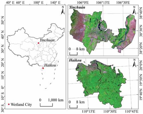
Yinchuan is the capital of the Ningxia Hui Autonomous Region. It is located in the north temperate zone, which has a the temperate continental climate. The population is 1.9 million people and the GDP was 196.44 billion yuan in 2020. The average annual rainfall is 185 mm and the average annual temperature is 8.5°C. As an inland, arid to semiarid city, Yinchuan has relatively rich wetland resources due to the Yellow River.

Haikou is the capital of Hainan Province. It is located on the northern edge of the low-latitude tropics i.e. 19°31′~20°04′N, and has a tropical monsoon climate. The population is 2.87 million people, and the GDP was 179.16 billion yuan in 2020. The average annual rainfall is 1600 mm, and the average annual temperature is 24°C. As a coastal city in a tropical region, it has abundant wetland resources. The coastal area is defined with a buffer zone 15 km inward from the coastline and a water depth of less than 25 m beyond the coastline (Mao et al. 2020).

The area of the municipal district in Yinchuan is 1805 km². The land area of Haikou is 2232 km², and the area including the seaside extension is 2745 km². The study area of Haikou includes the coastal expansion part with a seawater depth is less than 25 m because Haikou is a coastal city. The purpose for this is to ensure that coastal wetland types are not missed in wetland extraction. Haikou and Yinchuan have the same magnitude of area, population, and GDP, but their temperature and rainfall are significantly different. These two study areas with large environmental differences are conducive to demonstrating that the fine wetland extraction framework has better applicability.

2.2. Data

2.2.1. Satellite images and data preprocessing

The Sentinel series of satellite data from the European Space Agency has improved the spatial and temporal resolution, which has created new opportunities for wetland and land monitoring (Jia et al. 2021; Mahdianpari et al. 2019b). Sentinel-1 offers SAR data with a pixel spacing of 10 m, which is more sensitive to wetlands and is of great significance for wetland monitoring in areas covered by almost permanent cloud cover (Mahdianpari et al. 2019b). Sentinel-2 has optical remote sensing data, including 13 bands. Sentinel-2A and Sentinel-2B launched in 2015 and 2017, respectively, and can supply data with a revisit period of 2–5 days and with a 10-m spatial resolution (Jia et al. 2021). Therefore, we added Landsat-8 as supplemental data for wetland extraction for 2015. To mitigate the limitations that arise due to cloud cover, we applied selection criteria to cloud percentage (<20%) when producing a cloud-free composite from Sentinel-2 and Landsat-8 images (Mahdianpari et al. 2019b). On the Google Earth Engine (GEE) platform, the QA60 bitmask band (a quality flag band), which was provided in the metadata from Sentinel-2, was used to detect and mask out clouds and cirrus (Mahdianpari et al. 2019b). The BQA bitmask band, which was provided in the metadata from Landsat-8, was also used to select and mask out terrain occlusion and clouds.

2.2.2. Wetland and auxiliary data

Various wetland and land cover datasets used in this study are presented in Tables 1 and 2. These data were used to produce sample points, wetland classification, and validation results. There were some auxiliary datasets in this study, as Table 2 shows, used for wetland classification.

Table 1. The wetland datasets in this paper (“–” refers to data without spatial resolution or a specific year).

Product name	Wetland type	Time	Spatial resolution	References
1. Wetland type dataset
JRC Global Surface Water (JRC_GSW)	Water	1980 ~ 2020	30 m	Pekel et al. (2016)
HydroLAKES	Lake, Reservoir	–	1:100,000 ~ 1:250,000	Messager et al. (2016)
Global River Widths from Landsat (GRWL)	River	–	30 m	Allen and Pavelsky (2018)
Global Intertidal Change	Tidal flat	2015	30 m	Murray et al. (2019)
Global Saltmarsh	Coastal marsh	2015	1:10,000 ~ 1:4,000,000	Mcowen et al. (2017)
Mangrove map of China 2018 (MC2018)	Mangrove	2018	2 m	Zhang et al., (2021)
The POI data of the reservoir	Reservoir	–	–	Data download using the EasyPoi tool from Autonavi Map
Tidal Wetlands in East Asia (TWEA)	Mangrove, Coastal marsh, Tidal flat	2020	10 m	Zhang et al. (2022)
Mangroves of coastal China in 2020 (MC2020)	Mangrove	2020	30 m	National Geographic Resource Science SubCenter, National Earth System Science Data Center, National Science & Technology Infrastructure of China (http://gre.geodata.cn)
China’s surface water bodies, Large Dams, Reservoirs, and Lakes dataset(China-LDRL)	Lake, Reservoir	–	30 m	Wang et al. (2022)
2. Land cover dataset with wetland categories
ESA WorldCover (ESA_WC10)	Water, Marsh, Mangrove	2020	10 m	https://viewer.esa-worldcover.org/worldcover
Dynamic World (DW10)	Water, Flooded Vegetation	2015 ~ 2020	10 m	Brown et al. (2022)
GlobeLand 30	Wetland, Water	2020	30 m	http://www.globallandcover.com/home.html?type=data (Chen et al. (2015))
Global Land Cover with Fine Classification System at 30 m (GLC_FCS30)	Wetland, Water	2015, 2020	30 m	Zhang et al., (2021b);
Finer Resolution Observation and Monitoring-Global Land Cover(FROM_GLC30)	Water, Wetland	2015	30 m	http://data.ess.tsinghua.edu.cn/fromglc2015_v1.html

Table 2. Auxiliary data in this study.

Product name	References	Usage
Global Self-consistent, Hierarchical, High Geography Database-World Vector Shoreline (GSHHG-WVS)	https://www.soest.hawaii.edu/pwessel/gshhg/	identifying coastal areas
Global Relief Model ETOPO1 (ETOPO1)	https://www.ngdc.noaa.gov/mgg/global/	delimiting coastal expansion parts of coastal cities and identifying shallow marine waters
Global Reservoir and Dam Database (GRanD)	http://globaldamwatch.org/data/#core_global	delimiting coastal expansion identifying reservoirs
NASA SRTM Digital Elevation 30 m (SRTM-DEM)	Farr et al. (2007)	calculating features for wetland classification

2.3. Urban wetland classification system

The Ramsar definition of wetlands is widely accepted because it includes most wetland features (Mao et al. 2020). The wetland classification system used in this study is presented in Table 3 and follows the Chinese wetland classification national standard (GB/T 24708–2009) (Mao et al. 2020). This classification scheme contains 14 subcategories of wetland and 6 types for nonwetland.

Table 3. Urban wetland classification system for remote sensing (legend for the extracted example is show in Table A3).

3. Methodology

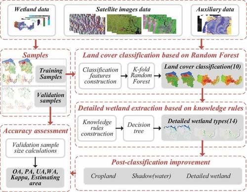
The framework of the fine wetland extraction method is shown in Figure 2, which mainly includes 5 parts, namely, 3.1. Training and validation sample construction; 3.2. Land cover classification based on random forest; 3.3. Detailed wetland type extraction based on knowledge rules; 3.4. Postclassification improvement; and 3.5. Accuracy assessment.

Figure 2. The framework of the fine wetland extraction method.

3.1. Training and validation sample construction

To balance the sample accuracy and the workload of sample collection and consider the difficulty of collecting different samples, we adopted different collection methods for wetland and nonwetland samples, as indicated in Figure 3. For the wetland samples, water and nonwater samples, we used different methods. For example, the water inundation frequency (WIF) data of JRC-GSW covering more than 80% were used as samples of stable water. Samples of water for Category II were identified by visual interpretation. Other nonwater samples for swamp, marsh, and beaches were generally difficult to collect. Therefore, we used a variety of methods to obtain these samples. First, we obtained the potentially nonwater wetland regions in which the WIF was more than 5% and less than 40% from 1980 to 2020 based on the JRC-GSW data. Then, the annual variation in the NDVI from the Collect Earth tool was used to determine the type of samples. The NDVI fluctuated between 0 and 0.8, the color in the growing season was green or turquoise, and in the nongrowing season, it was brown or reddish-brown, and the texture was rough and grainy, which can be regarded as swamp (Peng et al., 2021a). The NDVI of marsh fluctuated between 0 and 0.5, but some marsh was between 0 and 0.8, the color in the growing season was cyan or light cyan, and in the non-growing season was gray or reddish-brown, and the texture was relatively homogeneous (Peng et al., 2021a). Second, wetland data such as Global Intertidal Change, Global Saltmarsh, MC2018, TWEA, and ESA_WC10 wetland data could be used to collect wetland samples. At the same time, we also examined these wetland samples by visual interpretation based on Google Earth images or Sentinel-2 images. Finally, samples of nonwater wetlands for Category II were identified based on coastal areas.

Figure 3. Process of sample collection.

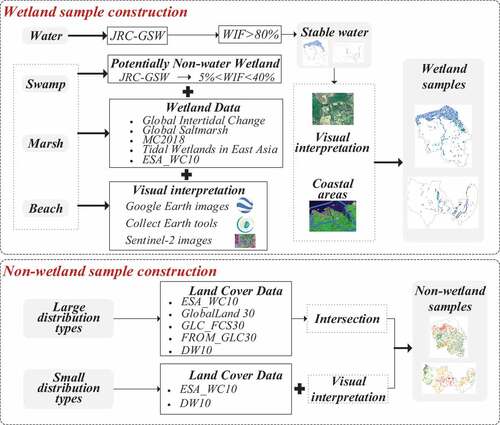
When a city is in the study area, there are some categories that exhibit a large distribution range and are concentrated, such as farmland and built area. Some categories display a small distribution scope and are scattered, such as bare land. For the nonwetland samples, we also used two methods to collect sample points for different types to increase the sample accuracy. A sample of large distribution types was collected by the intersection of multiple land cover data, such as ESA_WC10, DW10, GlobeLand 30, GLC_FCS30 and FROM_GLC30. The sample of small distribution types was collected by visual interpretation and the ESA WC10 and DW10 datasets.

We used the following constraints to determine the number of different types of samples. First, we determined the samples based on stratified random sampling. Second, to obtain more accurate wetlands, we ensured that the number of wetland and nonwetland samples were more balanced due to the study area being wetland city. Third, the number of training samples was not less than 100, and the verification samples were not less than 50 for one category. The calculation method of the number of verification samples is explained in Subsection 3.5 Accuracy assessment in detail. The samples used for 2020 wetland mapping were obtained through the above methods, but for the 2015 mapping, samples were transferred based on the relevant land cover data in 2020. Then, the sample was obtained based on the method described in Figure 3, when a large number of samples were needed. The wetland and nonwetland samples of Haikou and Yinchuan in 2015 and 2020 were obtained as indicated in Table 4.

Table 4. Training and validation sample size used for supervised classification in Haikou and Yinchuan.

		Haikou			Yinchuan
		Wetland	Nonwetland	Total	Wetland	Nonwetland	Total
2020	Training	3709	4080	7789	1117	1311	2428
	Validation	700	435	1135	448	749	1197
2015	Training	3427	3567	6994	1117	1386	2503
	Validation	661	453	1114	470	735	1205

3.2. Land cover classification based on random forest

3.2.1. Classification feature construction

There were four sets of features selected for wetland extraction, namely images, indices, texture, and topographic features, as indicated in Table 5. The image features mainly included the wettest, greenest, and median images. The wettest image and greenest image refer to the image synthesized at the moment when the modified Normalized Difference Water Index was the largest and the normalized difference vegetation index was the largest in one year, which was realized by qualityMosaic in the GEE (Jia et al. 2020). To ensure the consistency of the bands for OLI and MSI images, the band of MSI images only considered B2, B3, B4, B8, B11, and B12 in 2015 due to the OLI images not including red edge bands, i.e. B5, B6, B7 and B8A of MSI images. This was consistent with the OLI images. The median image captured the median value of the VV and VH bands of SAR images. The index features calculated the percentile and statistical composites of the normalized difference vegetation index (NDVI), enhanced vegetation index (EVI), normalized difference water index (NDWI), modified normalized difference water index (mNDWI), and automated water extraction index (AWEI_nsh) (Feyisa et al. 2014). The texture features were represented by a gray level co-occurrence matrix and the metrics of inverse difference moment, dissimilarity, contrast, entropy, angular second moment, sum average, variance, and correlation were calculated based on the NDVI. The topographic features of elevation, slope, and aspect were calculated based on SRTM data. The preprocessing tasks of all remote sensing images and building the collection of features were conducted on the GEE platform.

Table 5. Selected features for wetland extraction.

Feature I	Feature II	Description
Images features	Wettest image	The bands of MSI (Sentinel-2) images were calculated for the wettest image. (B2, B3, B4, B5, B6, B7, B8, B8A, B11, and B12 were used in 2020 and B2, B3, B4, B8, B11, and B12 were used in 2015)
	Greenest image	The bands of MSI (Sentinel-2) images were calculated for the greenest image. (B2, B3, B4, B5, B6, B7, B8, B8A, B11, and B12 were used in 2020 and B2, B3, B4, B8, B11, and B12 were used in 2015)
	Median image	The VV and VH bands of SAR (Sentinel-1) images were calculated for the median images in one year.
Index features	NDVI	Percentile composites (10%, 20%, 30, 40%, 50%, 60%, 70%, 80%, and 90%) Statistical composites (median, maximum, minimum, and standard deviation)
	EVI
	NDWI
	mNDWI
	AWEInsh
Texture features	Gray Level Co-occurrence matrix	Inverse difference moment, Dissimilarity, Contrast, Entropy, Angular second moment, Sum average, Variance, and Correlation
Topographic features	Elevation	Topographic features from SRTM-DEM data.
	Slope
	Aspect

3.2.2. K-fold random forest

The term k-fold random forest indicates that the training samples were trained k times based on the random forest (RF) method, and the most likely type of the k times results were used as the final classification results. This was to achieve a stable and robust wetland classification considering the complexity and diversity of wetlands. The RF is an enabled algorithm that can address multicollinearity well and avoid accuracy decrease due to feature redundancy, and, it is without assumptions of independence and normal distribution (Schulz et al. 2021; Peng et al., 2021b). In this study, for the RF classifier, we set the number of trees to 100 (nTree = 100), and the number of features in each tree was split into the square root of the total number of features (mTry = 11). Meanwhile, the training samples were trained 10 times (i.e. k = 10). Ten land cover classes including water, swamp, marsh, beach land, tree, grass, built area, dry land, paddy land, and bare ground were included in the analysis.

3.3. Detailed wetland type extraction based on knowledge rules

Knowledge rules can be understood as a series of rules based on existing expert knowledge or prior experience, which can be used to identify certain classes, e.g. land cover classes (Fitoka et al. 2020). The idea of decision trees has often been applied to remote sensing classification (Fitoka et al. 2020; Mao et al. 2020). Wetlands were subdivided based on the first rationale of classification, i.e. water, swamp, marsh, and beach land, and the determination rules can be seen in Table 6. Water bodies were classified using a decision tree, and the geometric features, i.e. compactness ratio/CR, elongation ratio/ER and related circumscribing circle /RCC) will also be used. The details of these geometric features are available at https://bit.ly/3Tor8J2 and can be calculated by the WhiteboxTools-ArcGIS tool (Lindsay 2016). The CR is defined as the polygon area divided by its perimeter and is an indicator of polygon shape complexity. The ER is 1 minus the short-axis length divided by the long-axis length, which is a linearity index of polygon features. The RCC is 1 minus the polygon’s area divided by the area of the smallest circumscribing circle, and if the index is closer to 0, the polygon feature is closer to the circle. We counted the distribution frequency of geometric features of linear water (as a river) and patchy water (as a lake) based on Chinese water system data. If 90% of linear water was larger than a certain value, such a value was used as the threshold for distinguishing between linear and patchy water. For canal/channels and agriculture ponds, the geometric features were analyzed in the same way, and the data were obtained visually to determine the rules as indicated in Table 6. The decision tree for the detailed classification of water is shown in Figure 4.

Figure 4. Decision tree for detailed classification of water.

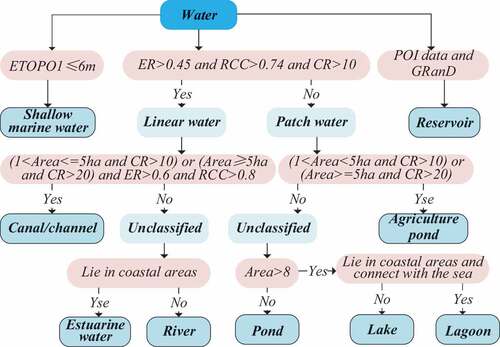
Table 6. Knowledge rules used for wetland classification.

Category of wetlands	Knowledge rules
Coastal swamp/Inland swamp	Swamp is located in coastal areas/ Swamp is located in noncoastal areas
Coastal marsh/Inland marsh	Marsh is located in coastal areas/ Marsh is located in noncoastal areas
Tidal flat/Inland beach	Beach is located in coastal areas/ Beach is located in non-coastal areas
Shallow marine water	The water areas are located in coastal areas and water depth of less than 6 m based on ETOPO1 data
Reservoir	Identified by the POI data of reservoir and GRanD
Linear water	ER>0.45 and RCC>0.74 and CR>10
Canal/channel	(1< Area≤5 ha and CR>10) OR (Area≥5 ha and CR>20)and ER>0.6 and RCC>0.8
River	Other unclassified areas and is located in noncoastal areas
Estuarine water	Other unclassified areas and is located in coastal areas
Patchy water	ER≤0.45 and RCC≤0.74 and CR≤10
Agriculture pond	(1< Area<5 ha and CR>10) OR (Area≥5 ha and CR>20)
Lagoon	Other unclassified areas and (Area >8 ha and is located in coastal areas and connected with the sea)
Lake	Other unclassified areas and Area >8 ha
Pond	Other unclassified areas and Area ≤8 ha

3.4. Postclassification improvement

Due to the complexity of wetlands, spectral information cannot accurately identify various wetland types. We needed to revise the classified data to improve the accuracy of wetland extraction. First, for urban wetlands, we considered that the urban cores i.e. the main built-up area of the city, generally have no cropland; therefore, we ensured the absence of both cropland and grassland in the urban cores. Urban shadows are easily misclassified as water, and we used built-up areas to mask them. In addition, when inaccuracies in the detailed classification of wetlands still remained, they were manually labeled.

3.5. Accuracy assessment

Based on stratified random sampling, we calculated the verification sample size using the following formula to ensure the rationality of the accuracy evaluation, and the sample size for each category was determined according to the area ratio for different categories(Olofsson et al. 2014).

(1) $N={\left(\frac{\sum W_i\times S_i}{S\left(\hat{O}\right)}\right)}^2$(1)

where N is the number of verification samples in one city, $S\left(\hat{O}\right)$ is the standard error of the estimated overall accuracy that we would like to achieve and is equal to 0.01, $W_i$ is the mapped proportion of the area of class i, $S_i$ is the standard deviation of stratum i, $S_i=\sqrt{U_i\left(1-U_i\right)}$, and $U_i$ is the user’s accuracy of class i that we would like to achieve. There are different accuracies due to the different difficulties of distinguishing different classes. In this paper, the $U_i$ value of different classes shown in Table A1 was determined based on existing research.

We used overall accuracy (OA), user’s accuracy (UA) and producer’s accuracy (PA) in the context of the error matrix to assess the accuracy (Olofsson et al. 2014). In this sense, the wetland accuracy (WA) was also calculated based on the error matrix which is the number of correctly classified pixels for the wetland class divided by the total number of pixels for the wetland class. The Kappa coefficient was used to measure the reliability of classification accuracy (Mao et al. 2020). In addition, we used the validation data of this study to verify the accuracy of other land cover datasets such as ESA_WC10, DW10, GlobalLand30, GLC_FCS30 and FROM_GLC30 in Haikou and Yinchuan.

4. Results

4.1. Classification accuracy and estimating area

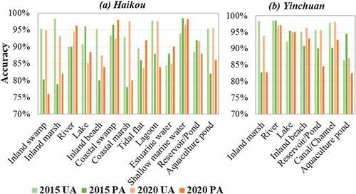
The wetland mapping results of Haikou and Yinchuan in 2015 and 2020 using the fine wetland extraction method were validated (Table A2). The OA and WA were greater than 88% and 87%, respectively, and the Kappa coefficient was above 87%. The OA for Haikou was 88.44% and 89.14% in 2015 and 2020, respectively, and the WA was 87.29% and 88.05%, respectively. The Kappa coefficient for Haikou was above 87%. The UA and PA for each wetland category were above 84% and 76% in Haikou (Figure 5 (a)). The accuracies for rivers, coastal swamp and shallow marine water were classified at higher accuracies and higher than 90%. The classification accuracy for marsh and inland swamp was low, which was primarily attributed to omission error. The OA for Yinchuan in 2015 and 2020 was 94.27% and 94.64%, respectively, and the WA was 91.91% and 89.93%, respectively. The Kappa coefficient for Yinchuan was above 93%.The UA and PA for each wetland category were above 86% and 82%, respectively, in Yinchuan (Figure 5 (b)). The accuracies for rivers, lakes, inland beaches, and canals/channels were classified at higher accuracies and higher than 90%. The accuracy for inland marsh was low due to omission error. Aquaculture ponds were classified at the lowest UA, in which they were misclassified as lakes or reservoirs/ponds in Yinchuan. The wetland classification accuracy of the two cities was generally better. The accuracy for Yinchuan was higher than that for Haikou, in which the types of wetlands in Haikou were more complex.

Figure 5. User’s accuracy (UA) and producer’s accuracy (PA) of different wetland categories in Haikou and Yinchuan.

The estimated area was calculated by the sample data, and a confidence level of 95% was presented for the area of each category (Table 7). The estimated wetland area in Haikou was 535.30 ± 198.78 km² in 2015 and 466.47 ± 153.75 km² in 2020. Coastal wetlands had the highest proportion for the wetlands of Haikou, and the estimated areas were 290.71 ± 79.84 km² and 246.16 ± 36.93 km² in 2015 and 2020, respectively. The estimated wetland area in Yinchuan was 114.54 ± 39.16 km² in 2015 and 133.77 ± 53.89 km² in 2020. Inland wetlands had the highest proportion among the wetlands in Yinchuan, and the estimated areas were 83.90 ± 23.62 km² and 84.64 ± 23.87 km² in 2015 and 2020, respectively. In addition, we found that the accuracy was higher, and the error range of the estimated area was smaller, which was mainly because the estimating area was calculated according to the sample.

Table 7. The estimated area (km²) in Haikou and Yinchuan in 2015 and 2020 (“–” indicates without the category in this city).

	Category	Haikou		Yinchuan
		2015	2020	2015	2020
Inland wetland	Inland swamp	59.48 ± 39.87	87.99 ± 51.84	–
	Inland marsh	64.37 ± 32.92	38.52 ± 27.04	31.35 ± 11.59	37.89 ± 16.03
	River	34.89 ± 24.01	24.96 ± 18.10	14.24 ± 0.47	13.99 ± 0.66
	Lake	9.40 ± 1.70	8.73 ± 1.49	20.51 ± 1.34	22.08 ± 1.26
	Inland beach	7.70 ± 6.18	8.87 ± 7.54	17.81 ± 10.23	10.68 ± 5.93
	Total	175.83 ± 104.67	169.06 ± 106.00	83.90 ± 23.62	84.64 ± 23.87
Coastal wetland	Coastal swamp	34.88 ± 22.33	26.09 ± 2.16	–
	Coastal marsh	56.74 ± 34.61	26.82 ± 15.43
	Tidal flat	18.31 ± 7.04	17.73 ± 2.32
	Lagoon	4.45 ± 1.11	4.60 ± 1.78
	Estuarine water	23.27 ± 5.44	21.96 ± 7.80
	Shallow marine water	153.06 ± 9.30	148.96 ± 7.44
	Total	290.71 ± 79.84	246.16 ± 36.93	–
Human-made wetland	Reservoir/Pond	37.54 ± 4.17	27.75 ± 2.53	7.62 ± 5.21	15.3 ± 10.94
	Canal/Channel	–		11.32 ± 9.07	12.6 ± 8.99
	Aquaculture pond	31.21 ± 10.09	23.5 ± 8.30	11.69 ± 1.26	21.22 ± 10.09
	Total	68.75 ± 14.26	51.24 ± 10.83	30.64 ± 15.54	49.13 ± 30.02
Summary		535.30 ± 198.78	466.47 ± 153.75	114.54 ± 39.16	133.77 ± 53.89

4.2 Comparison with other datasets

The example area for the detailed wetland mapping results in this study was compared with other wetland or land cover datasets (Figures 6 and 7). The detailed wetland mapping results were accurate and had a high resolution, and wetland types were more detailed compared with those in other datasets. The typical areas of mangroves (coastal swamp) and reservoirs in Haikou were selected for comparison with other mangroves and water datasets (Figure 6). The extraction range of mangroves was consistent with MC2020, TWEA2020 and MC2018 and more accurately distinguished the MSI image. The range and type of reservoir were more accurate than those of China-LDRL, HydroLAKES and JRC_GSW. The typical area of the detailed wetland in Haikou and Yinchuan was selected for comparison with other land cover datasets, and the detailed wetland mapping results were more accurate and wetland types more diverse (Figure 7). There were six wetland categories extracted in the typical areas of Yinchuan, while ESA_WC10 only had one category for water, and DW10 had two categories for flood vegetation and water. The aquaculture pond in the Haikou typical area was more accurate compared with ESA_WC10 and DW10. The validation data in this study verified the accuracy for other land cover datasets and obtained the OA for Haikou and Yinchuan in 2015 and 2020, as indicated in Table 8. We found that the accuracy of the detailed wetland mapping results was higher than that of the other land cover datasets, and it was more accurate, had a high resolution, and wetland categories more diverse.

Figure 6. Comparison between mangroves and reservoirs of detailed wetland types with other datasets in the example areas in Haikou in 2020.

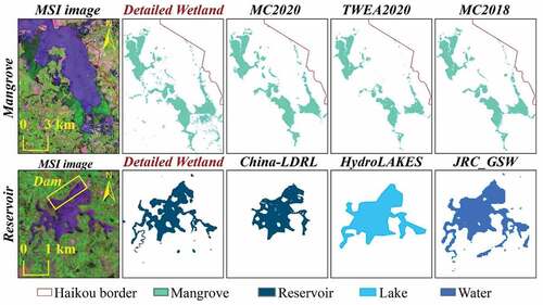
Figure 7. Comparison between detailed wetland mapping results with the land cover datasets for ESA_WC10 and WD10 in the example areas in Haikou and Yinchuan in 2020.

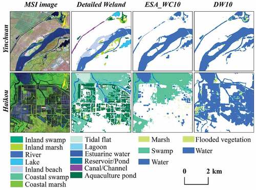
Table 8. OA for the detailed wetland datasets and other land cover datasets in Haikou and Yinchuan in 2015 and 2020 (“–” indicates without the dataset in this year).

Data	OA				Scale (m)	Wetland categories
	2020		2015
	Haikou	Yinchuan	Haikou	Yinchuan
Detailed Wetland	0.89	0.95	0.88	0.94	10	14
ESA_WC10	0.80	0.90	–	–	10	3
DW10	0.69	0.74	–	0.80	10	2
GLC_FCS30	0.58	0.76	0.61	0.69	30	2
GlobalLand30	0.61	0.76	–	–	30	2
FROM_GLC30	–	–	0.57	0.72	30	2

4.3 Detailed wetland type maps and analysis

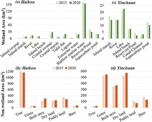
The detailed wetland results for Yinchuan and Haikou in 2015 and 2020 were mapped, as indicated in Figure 8. Wetlands in Haikou were mainly concentrated in coastal areas, and coastal wetlands were distributed widely. Yinchuan’s wetlands were concentrated in the center of the city, mainly lakes and rivers. The areas of wetlands and nonwetlands in the two cities in 2015 and 2020 were calculated (Figure 9). The wetland area in Haikou was 326.86 km² (13.43%) in 2015 and 308.58 km² (12.66%) in 2020. Yinchuan’s wetland area was 80.39 km² (4.46%) in 2015 and 74.15 km² (4.12%) in 2020. Of the 14 categories of wetlands, the shallow marine water had the largest area in Haikou, and lake area was largest in Yinchuan. The area for most wetland categories in 2020 was slightly lower than that in 2015 in the two cities, and the coastal swamp (mangrove) in Haikou increased significantly. This may be related to the development of artificial protection and restoration projects of mangroves (Jia et al. 2018). For the nonwetland areas, tree area was the largest in Haikou and cropland (dry land and paddy land) was the largest in Yinchuan. The built area in nonwetland areas increased, which may be the reason for the slight decrease in wetlands.

Figure 8. Detailed wetland type maps of Haikou and Yinchuan in 2015 and 2020.

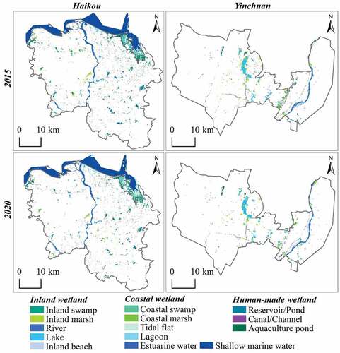
Figure 9. Areas of different categories of wetlands (a, c) and nonwetlands (b, d) in Haikou and Yinchuan.

5. Discussion

5.1. Advantages and feasibility of the fine wetland extraction framework

The fine wetland extraction framework based on random forest and knowledge rules in this paper not only ensured the extraction accuracy of urban wetlands but also obtained more detailed wetland-related land cover classes. The fine wetland extraction framework considered the complexity of wetland categories and the limitations of remote sensing data. First, the wetland categories with large spectral differences were obtained based on the random forest method, such as water, swamps, marshes, and beaches. Then, the detailed wetland categories such as rivers, lakes, reservoirs, estuary waters, and aquaculture ponds, were obtained based on the knowledge rules which considered the distribution area and shape characteristics. Compared with traditional visual interpretation, this method greatly improved the efficiency of wetland extraction. That is, the combined method could obtain more abundant data on wetland types compared with the single wetland extraction method (Amani et al. 2019; Ludwig et al. 2019). In addition, the sample and classification features provided better feasibility for the extraction of wetlands. The stable sample came from the intersection of multiple datasets, which ensured the accuracy of samples and reduced the workload in the field, which seems to be a good foundation for wetland extraction. The classification features considered the image features, index features, texture features and topographic features to extract wetlands, and both optical and radar images were used to better identify wetland features. Abundant remote sensing data also provided great feasibility for wetland mapping. Sentinel data have higher spatial resolution and shorter temporal resolution. In space, clearer data can be obtained, and in time, dense time series remote sensing data can more easily highlight wetland characteristics and realize wetland extraction. In addition, the GEE platform provides good support for the preprocessing of these remote sensing data, which greatly reduces the data processing work.

5.2. Uncertainties

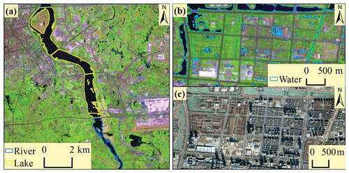
This framework is very helpful for extracting fine wetland categories, there are still some issues that need to be considered in wetland extraction. There are many uncertainties in the wetland extraction process, mainly due to the complexity and diversity of wetland types. For example, building shadows in cities were easily misclassified as water bodies (Figure 10b,). Although the building shadows in this study were corrected in the postclassification process, it is still necessary to research how to remove building shadows automatically. Second, since the classification of rivers and lakes was based on geometric features, they were certainly affected by the complexity of the urban environment. For example, the integrity of rivers was affected by bridges (Figure 10a). In this case, we also made a manual revision in the postclassification. We realize that such factors did have an impact on the fine extraction of wetlands; therefore, they deserve further attention.

Figure 10. Uncertainty example. (a) MSI image (R: Band12, G: Band8, B: Band4) and classification results based on geometric features in Haikou. (b) MSI image (R: Band12, G: Band8, B: Band4) and water bodies in Yinchuan. (c) Google Earth image of the same location as (b) in Yinchuan.

5.3. Potential application

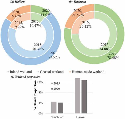
This method can be widely used for mapping wetland cities with higher spatial resolution and detailed types. This method can monitor the status of urban wetlands in real time and is a support for urban development and wetland protection. At the same time, from the perspective of remote sensing, this approach can be used to support the proposal accompanying the creation of a new wetland city. We calculated the proportions of coastal, inland and human-made wetlands, and the corresponding wetland rates in the two studied cities. Figure 11 shows that more than 70% of the wetlands in Haikou were coastal wetlands, of which shallow marine waters accounted for the most. For the changes from 2015 to 2020, the proportion of coastal and inland wetlands increased, while the human-made wetlands decreased. More than 70% of the wetlands in Yinchuan were inland wetlands. It was also found that the proportion of inland wetlands increased, and human-made wetlands decreased from 2015 to 2020. For the wetland rates in the two cities, the wetland rates in 2020 were slightly lower than those in 2015, but the wetland rates were always greater than 4% in Yinchuan and greater than 12% in Haikou (Figure 11c). We found that the wetland rates of the two cities decreased, but the proportion of natural wetlands increased. This shows that the development of wetlands in Haikou and Yinchuan is better. These indicators are important for wetland city certification, and the method can also provide significant support for Wetland City Accreditation work.

Figure 11. The proportion of inland, coastal and human-made wetlands in wetlands (a, b) and the wetland proportion in (c) Haikou and Yinchuan.

6. Conclusions

Rich wetland types and high wetland data are very important for understanding urban wetland status and monitoring urban wetland environments. This study proposed a new framework for fine wetland extraction that mainly used random forests and knowledge rules, and mapped the wetlands in Haikou and Yinchuan in 2015 and 2020. The obtained dataset contained 14 wetland types at a 10-m spatial resolution.

The overall accuracy and Kappa values of wetland extraction were higher than 88% and 87%, respectively. The UA and PA for each wetland category were above 84% and 76%, respectively, in Haikou and Yinchuan. The extraction accuracy of wetland categories such as rivers, lakes, estuarine waters, shallow marine water, and coastal swamps was high. Compared with other wetland-related datasets, our dataset of detailed wetland types has a higher spatial resolution, better accuracy, and more classes of wetland types.

The wetland area in Haikou was greater than 300 km², and wetlands accounted for more than 12%. The wetland area in Yinchuan was greater than 70 km², accounting for more than 4%. By comparing the wetlands in 2015 and 2020, it was found that most wetland types in the two cities in 2020 declined slightly, but the coastal woody swamps (mangroves) in Haikou increased significantly.

The fine wetland extraction framework was applied well to the two cities and will be applied to fine wetland extraction and real-time wetland environmental monitoring in more wetland cities in the future. This will play an important role in supporting the protection and development of urban wetlands.

Credit author statement

Wang Xiaoya: Conceptualization, software, and writing - original draft

Jiang Weiguo: Funding acquisition, Supervision

Peng Kaifeng: Methodology

Li Zhuo: Writing - Review & Editing

Rao Pinzeng: Writing - Review & Editing

Acknowledgements

The researchers would like to thank anonymous reviewers for their suggestions for improving the language and structure of the article.

Disclosure statement

No potential conflict of interest was reported by the author(s).

Data availability statement

The detailed wetland data of Yinchuan and Haikou in 2015 and 2020 are available in Zenodo (https://doi.org/10.5281/zenodo.7006663).

Additional information

Funding

This work was supported by the National Natural Science Foundation of China Grant U21A2022, Grant U1901219, Grant42071393 under Grants U21A2022, U1901219 and 42071393.

Appendix

Table A1. The $U_i$ value of different classes.

Classes	$U_i$	Classes	$U_i$
Inland swamp	0.80	Shallow marine water	0.90
Inland marsh	0.80	Reservoir/Pond	0.80
River	0.90	Canal/Channel	0.80
Lake	0.85	Aquaculture pond	0.80
Inland beach	0.85	Trees	0.90
Coastal swamp	0.90	Grass	0.85
Coastal marsh	0.85	Built area	0.90
Tidal flat	0.85	Dry land	0.85
Lagoon	0.80	Paddy land	0.85
Estuarine water	0.90	Bare	0.9

Table A2. Classification accuracy of different categories for Haikou and Yinchuan (“–” refers to without the category in this city).

	Category	Haikou				Yinchuan
		2015		2020		2015		2020
		UA	PA	UA	PA	UA	PA	UA	PA
Inland wetland	Inland swamp	95.35%	80.39%	95.00%	76.00%	–
	Inland marsh	98.36%	78.95%	93.18%	82.00%	98.41%	82.67%	93.94%	82.67%
	River	90.00%	90.00%	94.44%	96.23%	98.55%	98.55%	97.18%	97.18%
	Lake	90.74%	96.08%	85.19%	88.46%	92.13%	95.35%	95.00%	95.00%
	Inland beach	95.24%	80.00%	87.50%	84.00%	95.16%	90.77%	96.36%	92.98%
Coastal wetland	Coastal swamp	93.33%	96.55%	92.45%	98.00%	–
	Coastal marsh	92.86%	78.00%	97.56%	80.00%
	Tidal flat	89.58%	86.00%	83.64%	92.00%
	Lagoon	97.78%	88.00%	97.67%	84.00%
	Estuarine water	84.62%	88.00%	84.91%	90.00%
	Shallow marine water	94.03%	98.44%	96.49%	98.21%
Human-made wetland	Reservoir/Pond	88.46%	92.00%	91.67%	88.00%	95.74%	90.00%	95.65%	84.64%
	Canal/Channel	–				97.87%	90.20%	98.08%	92.73%
	Aquaculture pond	95.35%	82.00%	95.56%	86.00%	86.42%	94.59%	87.04%	82.46%
Non-wetland	Tree	82.55%	93.18%	84.44%	95.00%	98.31%	98.31%	98.28%	95.00%
	Grass	80.36%	90.00%	87.04%	82.46%	96.50%	96.50%	96.48%	98.46%
	Built area	92.77%	95.06%	89.04%	98.48%	91.73%	97.60%	90.00%	99.31%
	Dry land	71.43%	80.00%	80.77%	84.00%	95.41%	93.97%	94.24%	96.26%
	Paddy land	77.50%	88.57%	83.72%	96.00%	90.12%	92.41%	92.86%	98.73%
	Bare	88.00%	88.00%	94.34%	83.33%	91.03%	97.26%	98.70%	95.00%
	WA	87.29%		88.05%		91.91%		89.93%
	OA	88.44%		89.14%		94.27%		94.64%
	Kappa	87.71%		87.52%		93.65%		94.04%

Table A3. Legend for different categories about the extracted example.

References

- Allen, G. H., and T. M. Pavelsky. 2018. “Global Extent of Rivers and Streams.” Science 361 (6402): 585–588. doi:10.1126/science.aat0636.
- Amani, M., S. Mahdavi, M. Afshar, B. Brisco, W. Huang, S. Mohammad Javad Mirzadeh, L. White, S. Banks, J. Montgomery, and C. Hopkinson. 2019. “Canadian Wetland Inventory Using Google Earth Engine: The First Map and Preliminary Results.” Remote Sensing 11 (7): 842. doi:10.3390/rs11070842.
- Brown, C. F., S. P. Brumby, B. Guzder-Williams, T. Birch, S. B. Hyde, J. Mazzariello, W. Czerwinski, et al. 2022. “Dynamic World, near real-time Global 10 M Land Use Land Cover Mapping.” Scientific Data 9 (1): 251. doi:10.1038/s41597-022-01307-4.
- Chen, J., J. Chen, A. Liao, X. Cao, L. Chen, X. Chen, C. He, et al. 2015. “Global Land Cover Mapping at 30m Resolution: A POK-based Operational Approach.” ISPRS Journal of Photogrammetry and Remote Sensing 103 7–27. doi:10.1016/j.isprsjprs.2014.09.002.
- Farr, T. G., P. A. Rosen, E. Caro, R. Crippen, R. Duren, S. Hensley, M. Kobrick, et al. 2007. “The Shuttle Radar Topography Mission.” Reviews of Geophysics 45 (2). doi:10.1029/2005RG000183.
- Feyisa, G. L., H. Meilby, R. Fensholt, and S. R. Proud. 2014. “Automated Water Extraction Index: A New Technique for Surface Water Mapping Using Landsat Imagery.” Remote Sensing of Environment 140: 23–35. doi:10.1016/j.rse.2013.08.029.
- Fitoka, E., M. Tompoulidou, L. Hatziiordanou, A. Apostolakis, R. Höfer, K. Weise, and C. Ververis. 2020. “Water-related Ecosystems’ Mapping and Assessment Based on Remote Sensing Techniques and Geospatial Analysis: The SWOS National Service Case of the Greek Ramsar Sites and Their Catchments.” Remote Sensing of Environment 245: 111795. doi:10.1016/j.rse.2020.111795.
- Jamali, A., M. Mahdianpari, B. Brisco, J. Granger, F. Mohammadimanesh, and B. Salehi. 2021. “Deep Forest Classifier for Wetland Mapping Using the Combination of Sentinel-1 and Sentinel-2 Data.” GIScience & Remote Sensing 58 (7): 1072–1089. doi:10.1080/15481603.2021.1965399.
- Jia, M., D. Mao, Z. Wang, C. Ren, Q. Zhu, X. Li, and Y. Zhang. 2020. “Tracking long-term Floodplain Wetland Changes: A Case Study in the China Side of the Amur River Basin.” International Journal of Applied Earth Observation and Geoinformation 92: 102185. doi:10.1016/j.jag.2020.102185.
- Jia, M., Z. Wang, D. Mao, C. Ren, C. Wang, and Y. Wang. 2021. “Rapid, Robust, and Automated Mapping of Tidal Flats in China Using Time Series Sentinel-2 Images and Google Earth Engine.” Remote Sensing of Environment 255: 112285. doi:10.1016/j.rse.2021.112285.
- Jia, M., Z. Wang, Y. Zhang, D. Mao, and C. Wang. 2018. “Monitoring Loss and Recovery of Mangrove Forests during 42 Years: The Achievements of Mangrove Conservation in China.” International Journal of Applied Earth Observation and Geoinformation 73: 535–545. doi:10.1016/j.jag.2018.07.025.
- Lindsay, J. B. 2016. “Whitebox GAT: A Case Study in Geomorphometric Analysis.” Computers & Geosciences 95: 75–84. doi:10.1016/j.cageo.2016.07.003.
- Ludwig, C., A. Walli, C. Schleicher, J. Weichselbaum, and M. Riffler. 2019. “A Highly Automated Algorithm for Wetland Detection Using multi-temporal Optical Satellite Data.” Remote Sensing of Environment 224: 333–351. doi:10.1016/j.rse.2019.01.017.
- Mabwoga, S. O., and A. K. Thukral. 2014. “Characterization of Change in the Harike Wetland, a Ramsar Site in India, Using Landsat Satellite Data.” SpringerPlus 3 (1): 576. doi:10.1186/2193-1801-3-576.
- Mahdianpari, M., H. Jafarzadeh, J. E. Granger, F. Mohammadimanesh, B. Brisco, B. Salehi, S. Homayouni, et al. 2020. “A large-scale Change Monitoring of Wetlands Using Time Series Landsat Imagery on Google Earth Engine: A Case Study in Newfoundland.” GIScience & Remote Sensing 57 (8): 1102–1124. doi:10.1080/15481603.2020.1846948.
- Mahdianpari, M., B. Salehi, F. Mohammadimanesh, S. Homayouni, and E. Gill. 2019. “The First Wetland Inventory Map of Newfoundland at a Spatial Resolution of 10 M Using Sentinel-1 and Sentinel-2 Data on the Google Earth Engine Cloud Computing Platform.” Remote Sensing 11 (1): 43. doi:10.3390/rs11010043.
- Mao, D., Z. Wang, B. Du, L. Li, Y. Tian, M. Jia, Y. Zeng, et al. 2020. “National Wetland Mapping in China: A New Product Resulting from object-based and Hierarchical Classification of Landsat 8 OLI Images.” ISPRS Journal of Photogrammetry and Remote Sensing 164 11–25. doi:10.1016/j.isprsjprs.2020.03.020.
- Mcowen, C. J., L. V. Weatherdon, J.-W. Van Bochove, E. Sullivan, S. Blyth, C. Zockler, D. Stanwell-Smith, et al. 2017. “A Global Map of Saltmarshes.” Biodiversity Data Journal 5 e11764. doi:10.3897/BDJ.5.e11764.
- Messager, M. L., B. Lehner, G. Grill, I. Nedeva, and O. Schmitt. 2016. “Estimating the Volume and Age of Water Stored in Global Lakes Using a geo-statistical Approach.” Nature Communications 7 (1): 13603. doi:10.1038/ncomms13603.
- Murray, N. J., S. R. Phinn, M. DeWitt, R. Ferrari, R. Johnston, M. B. Lyons, N. Clinton, et al. 2019. “The Global Distribution and Trajectory of Tidal Flats.” Nature 565 (7738): 222–225. doi:10.1038/s41586-018-0805-8.
- Olofsson, P., G. M. Foody, M. Herold, S. V. Stehman, C. E. Woodcock, and M. A. Wulder. 2014. “Good Practices for Estimating Area and Assessing Accuracy of Land Change.” Remote Sensing of Environment 148: 42–57. doi:10.1016/j.rse.2014.02.015.
- Pekel, J.-F., A. Cottam, N. Gorelick, and A. S. Belward. 2016. “High Mapping of Global Surface Water and Its long-term Changes.” Nature 540 (7633): 418–422. doi:10.1038/nature20584.
- Peng, K., W. Jiang, P. Hou, Z. Ling, Z. Niu, D. Mao, and Z. Huang. 2021a. “Dense Wetland Sample Production at Large Scale by Combining multi-source Thematic Datasets and Visual Interpretation.” National Remote Sensing Bulletin 1–13. doi:10.11834/jrs.20211152.
- Peng, K., W. Jiang, Z. Ling, P. Hou, and Y. Deng. 2021b. “Evaluating the Potential Impacts of Land Use Changes on Ecosystem Service Value under Multiple Scenarios in Support of SDG Reporting: A Case Study of the Wuhan Urban Agglomeration.” Journal of Cleaner Production 307: 127321. doi:10.1016/j.jclepro.2021.127321.
- Schulz, D., H. Yin, B. Tischbein, S. Verleysdonk, R. Adamou, and N. Kumar. 2021. “Land Use Mapping Using Sentinel-1 and Sentinel-2 Time Series in a Heterogeneous Landscape in Niger, Sahel.” ISPRS Journal of Photogrammetry and Remote Sensing 178: 97–111. doi:10.1016/j.isprsjprs.2021.06.005.
- Wang, X., X. Xiao, Y. Qin, J. Dong, J. Wu, and B. Li. 2022. “Improved Maps of Surface Water Bodies, Large Dams, Reservoirs, and Lakes in China.” Earth System Science Data Discussions 1–44. doi:10.5194/essd-2021-400.
- Yang, J., and X. Huang. 2021. “The 30 M Annual Land Cover Dataset and Its Dynamics in China from 1990 to 2019.” Earth System Science Data 13 (8): 3907–3925. doi:10.5194/essd-13-3907-2021.
- Zanaga, D., R. Van De Kerchove, W. De Keersmaecker, N. Souverijns, C. Brockmann, R. Quast, J. Wevers, et al. 2021. “ESA WorldCover 10 M 2020 v100.” Nature Communications 12 (1). doi:10.5281/zenodo.5571936.
- Zhang, T., S. Hu, Y. He, S. You, X. Yang, Y. Gan, and A. Liu. 2021a. “A Fine-Scale Mangrove Map of China Derived from 2-Meter Resolution Satellite Observations and Field Data.” ISPRS International Journal of Geo-Information 10 (2): 92. doi:10.3390/ijgi10020092.
- Zhang, X., L. Liu, X. Chen, Y. Gao, S. Xie, and J. Mi. 2021b. “GLC_FCS30: Global land-cover Product with Fine Classification System at 30 m Using time-series Landsat Imagery.” Earth System Science Data 13 (6): 2753–2776. doi:10.5194/essd-13-2753-2021.
- Zhang, Z., N. Xu, L. Yangfan, and Y. Li. 2022. “Sub-continental-scale Mapping of Tidal Wetland Composition for East Asia: A Novel Algorithm Integrating Satellite tide-level and Phenological Features.” Remote Sensing of Environment 269: 112799. doi:10.1016/j.rse.2021.112799.
- Zhao, C., and C.-Z. Qin. 2020. “10-m Mangrove Maps of China Derived from multi-source and multi-temporal Satellite Observations.” ISPRS Journal of Photogrammetry and Remote Sensing 169: 389–405. doi:10.1016/j.isprsjprs.2020.10.001.
Appendix
Table A1. The value of different classes.