Can time-series Sentinel images be used to properly identify wetland plant communities?

ABSTRACT

Understanding the distribution of wetland plant communities is critical to biodiversity conservation and wetland habitat sustainable management, especially for migratory birds. However, limited road accessibility and low spectral discriminability make the mapping of wetland plant communities inadequate for wetland health assessment, necessitating the improvement of classification methods. In this study, we proposed a random forest classifier that combined multi-source remote sensing features for wetland plant community classification and evaluated this method for the Momoge Ramsar wetland site (MRWS) in China. The major result of this work was that the phenological and time-series features based on Sentinel-2 images were the most valuable discriminators for wetland plant community classification in the MRWS. The SAR_sum extracted from Sentinel-1 images also had high importance for classification. Moreover, the spatial pattern of different wetland plant communities was revealed, and the resultant classification map had a high overall accuracy (91.3%) and Kappa coefficient (0.90). And the six important features prompted the classification accuracy to reach 84.8%. In 2020, the total coverage area of natural wetland plant communities in MRWS reached 628.5 km² (42.1%), of which Carex meyeriana distributed the most widely, followed by Suaeda glauca, Phragmites australis, Typha orientalis, and Scirpus triquater. The findings of this study can provide scientific decision-making support for the protection and management of migratory birds and plants in the MRWS. The proposed method employed freely available Sentinel 1/2 satellite images and fully automated programs on Google Earth Engine, and has guiding significance for large-scale and long-time-series wetland classification.

KEYWORDS:

• Wetland plant community
• Google Earth Engine
• random forest classifier
• phenological feature
• Sentinel time-series image

1. Introduction

Plant communities are considered the basic unit of wetlands, which provide ecosystem functions and services such as water quality purification and biological diversity conservation (Mao et al. 2022; Mitsch 1996; Rodwell, Evans, and Schaminée 2018). Accurate spatial distribution information of plant communities is thus essential for the health assessment and sustainable habitat management of wetlands (Mao et al. 2020; Rapinel et al. 2019). However, the dynamicity and complexity of the wetland environment make it very difficult for the fine classification of wetland plant communities based on remote sensing technology (Mahdavi et al. 2018; Zhang et al. 2011), which has become a restricting factor affecting the scientific management of wetlands. Therefore, it is urgent to develop an effective wetland plant community classification method.

Due to spectral similarity, it is difficult to obtain satisfactory wetland plant communities classification accuracy using multispectral images (Martínez-López et al. 2014; Zhang et al. 2011). Previous studies indicated that hyperspectral images have a unique advantage in spectral resolution for wetland plant communities classification (Belluco et al. 2006; Du et al. 2021; Schmidt and Skidmore 2003; Yang et al. 2022). However, cloudy conditions and high costs limit the application of hyperspectral images in large-scale research (Kumar and Sinha 2014; Pengra, Johnston, and Loveland 2007). Synthetic-aperture radar (SAR) data is considered an important data source for wetland classification. SAR sensors can observe wetlands under various weather conditions (Henderson and Lewis 2008; Wang et al. 2023) and obtain valuable information about the water and ground conditions under vegetation canopies (Li, Chen, and Touzi 2007). Another way to minimize weather effects and research costs is to use time-series data, which are considered to have application potential for wetland plant community classification (Mao et al. 2018; Sun et al. 2021; Mahdianpari et al. 2020; Zhou et al. 2022). For example, some studies have used the life history information of different plant species for wetland classification (Luo et al. 2017). Other studies have added digital elevation model (DEM) data to wetland classification procedures to improve the accuracy of the resultant map (Hladik, Schalles, and Alber 2013; Kloiber et al. 2015; Li and Chen 2005; Rummell et al. 2022). Therefore, fine wetland classification based on multi-source remote sensing images and time-series data has become the mainstream trend of current research.

In recent years, the rapid development of remotely sensed big data and cloud computing has provided technical support for the processing of multi-source data and the calculation of time-series features (Gorelick et al. 2017). It is well known that Google Earth Engine (GEE) has been widely used in numerous wetland classification studies (Chen et al. 2017; Dong et al. 2020; Mahdianpari et al. 2018). On the one hand, users can directly access free Landsat, Sentinel-1, and Sentinel-2 satellite images on GEE (Amani et al. 2019a), and there is no need to download large satellite images or allocate expensive computers for the extraction of time-series features. On the other hand, many predefined algorithms are easy to call and modify for cloud-based image processing and classification. Among the various algorithms, supervised machine learning methods are often used in wetland classification, such as support vector machines (SVMs), decision trees (DTs), and random forests (RFs) (Sanchez-Hernandez, Boyd, and Foody 2007). When solving multiple-category classification problems, the algorithm of the tree structure is more advantageous than that of SVM. As a collection of multiple DTs, the RF model is more stable than the DT model, so the performance of the RF model is often better than the DT model in auto classification (Correll et al. 2019; Mahdianpari et al. 2017). The use of an RF model can be divided into two categories: object-based and pixel-based. At present, the object-based image analysis (OBIA) of plant community scale still faces challenges on GEE. In order to accurately distinguish plant community types in complex wetlands, a smaller segmentation scale is often required, which means a considerable amount of calculation (Dronova 2015). However, many mature pixel-based methods are generally simple and run faster than OBIA. Moreover, they can clearly indicate the contribution degree of each feature to the classification.

The Wetlands of International Importance are essential for the biological diversity protection of global migratory birds. Different birds rely on different plant communities in the processes of foraging, resting, and breeding (Zhang et al. 2011). For example, the Phragmites australis, Carex meyeriana, Scirpus triquater, Suaeda glauca, and Typha orientalis communities provide habitat and food sources for many migratory birds such as Cygnus columbianus, Grus leucogeranus, Grus monachal, and Grus japonensis in the Momoge Ramsar wetland site (MRWS), located in the East Asian-Australasian Flyway (Wen et al. 2020). In this study, we used the MRWS as the study area. Based on the Sentinel time-series and DEM data, a novel classification method was proposed to achieve wetland plant classification at community scale. The specific goals were as follows: (i) to analyze the separability of plant communities characterized by different features; (ii) to perform RF classification and analyze the importance of different features; and (iii) to reveal the distribution patterns of different wetland plant communities based on post-processing classification results. We also provided scientific suggestions for the protection and management of migratory birds and plants in the MRWS.

2. Materials and methods

2.1. Study area

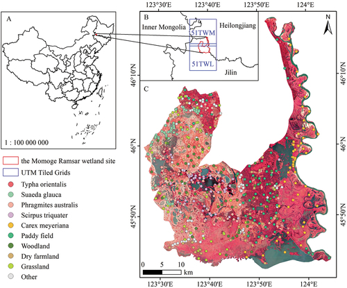
The Momoge Nature Reserve, established in 1981, was designated as Wetlands of International Importance (No. 2188) in 2013, covering an area of 1492 km² and spanning 45°42′33″ to 46°17′59″ N and from 123°27′09″ to 124°04′32″ E (Figure 1). The MRWS is a very important site for the foraging and perching of the water birds in the East Asian-Australasian Flyway. At the same time, it is essential for the ecological environment of the western Songnen Plain. The rich wetland plants and migratory bird resources make MRWS has an international importance in studies of wetland ecology and protection. Grus leucogeranus, which was identified as “Critically Endangered” by the International Union for Conservation of Nature Red List of Threatened Species (Jiang et al. 2016), is the key protected migratory bird of the MRWS. Plant communities in the MRWS such as Typha orientalis (TO), Suaeda glauca (SG), and Scirpus triquater (ST) are the places where Grus leucogeranus often live and forage (He et al. 2002). The Anatidae waterbirds, represented by Cygnus columbianus, mainly eat the tender leaves of Carex meyeriana (CM) and the rhizomes of Phragmites australis (PA). Except for fish, the scions of PA and the seeds of SG and ST are all food sources of Grus japonensis (Liu et al. 2016; Wang et al. 2020).

Figure 1. General situation of the study area. (A) geographic location of the MRWS in China; (B) the Sentinel-2 coverage for the MRWS; (C) sample distribution pattern with a background of a Sentinel-2 MSI standard false-color image (R: 8, G: 4, B: 3).

2.2. Dataset

2.2.1. Remote sensing images

Considering their high spatial, temporal, and spectral resolutions, the Sentinel-2 Multispectral Instrument (MSI) Level-2A images on GEE were employed in this study. A total of 290 scenes of Sentinel-2 images covering the study area during 2020 were collected. The growing season of vegetation in this region is from May to October, while the other months are regularly covered by snow. Therefore, total 26 scenes of Sentinel-1 Level-1 ground range detected (GRD) SAR images in Interferometric Wide swath mode with 10-meter resolution and VV-VH polarization covering the study area from May to October 2020 on GEE were employed. In addition, the PIE-Engine Cloud Platform shared the 12.5-meter resolution DEM data obtained by the phased-array L-band SAR of the Advanced Land Observing Satellite (ALOS) in 2011. In this paper, we downloaded the DEM data from PIE-Engine locally and then uploaded it to GEE to participate in wetland classification.

2.2.2. Sample data

We conducted field investigations on the MRWS from 23 to 27 July 2020. We used a portable handheld Global Positioning System (GPS) device with sub-meter accuracy to locate the distribution of wetland plant types in shallow water areas. We also took aerial photography of some wetlands in deep water areas using an unmanned aerial vehicle (UAV) and then interpreted the obtained images to expand the number of wetland plant samples. In addition, we directly selected the sample points of other surface coverage types such as woodland, grassland, farmland, buildings, and bare land by comparing images of Sentinel-2 and Google Earth. Finally, we formulated a classification system (Table 1) that contains five wetland plant community types (TO, SG, PA, ST, and CM) and five other types (Paddy field, Woodland, Dry farmland, Grassland, and Other). It should be noted that the class of “Other” includes buildings, roads, and bare land.

Table 1. Number of training and validation samples for each class in the classification system.

Class	Training Samples Pixels	Validation Samples Pixels	Total Samples Pixels
Typha orientalis	37	21	58
Suaeda glauca	34	25	59
Phragmites australis	37	23	60
Scirpus triquater	33	24	57
Carex meyeriana	26	27	53
Paddy field	32	26	58
Woodland	37	23	60
Dry farmland	34	26	60
Grassland	39	20	59
Other	36	25	61

2.3. Methods

Firstly, we preprocessed the three kinds of acquired satellite images, and the phenological, time-series, polarization, and terrain features were extracted to analyze the separability of different plant communities. Secondly, an RF model based on sample data and feature variables was used for plant community classification and accuracy assessment of the MRWS. Finally, the post-processed classification results were used to analyze the spatial pattern of different wetland plant communities. The overall classification workflow is shown in Figure 2.

Figure 2. The general framework of wetland plant community classification.

2.3.1. The methods to analyze the separability of plant communities

Remote sensing images preprocess

The same-period Sentinel-2 images from the 51TWM and 51TWL tiles seen in Figure 1B had the same time attribute, which was used as a basis for a batch mosaic (Figure 2). Then, the “ee.image.clip()” function was used to clip the mosaiced Sentinel-2 image collection. Afterward, an open-source code of GEE was used to remove cloud pixels of Sentinel-2 images because numerous cloud pixels are the main challenge for wetland classification using time-series methods (Sun et al. 2021). In addition, we also masked the water body of the study area because this study focused on the classification of the wetland plant community. Specifically, to ensure all plant cover pixels can be retained as much as possible when we extracted the water mask using the threshold method, the Sentinel-2 Normalized Difference Water Index (NDWI) images from 20 July to 20 August 2020 were composited with a median value function because the plant cover range reached the maximum during this period. Here, we tested a range of cutoff values and determined that −0.23 best correlated with reality. The formula to calculate NDWI is as follows:

(1) $NDWI=\frac{B8-B3}{B8+B3},$(1)

The Sentinel-1 GRD SAR data stored in GEE were all preprocessed, which included thermal noise removal, orbit file correction, filtering, radiometric calibration, and Doppler terrain correction. In addition, speckle reduction is a necessary preprocessing step for the use of SAR imagery (Li, Chen, and Touzi 2007). In this study, the speckle of Sentinel-1 images was reduced by a 7 × 7 refined Lee filter, which was implemented by Guido Lemoine and has been widely used in previous studies (Amani et al. 2019a). Finally, the DEM data were resampled to 10-meter resolution using a bilinear interpolation function and were reprojected to the “World Geodetic System 1984 (EPSG:4326)” to ensure that all remote sensing data could be used together.

Multi-source features extraction

Based on the preprocessed Sentinel-2 images, pixel-based Normalized Difference Vegetation Index (NDVI), Inverted Red-Edge Chlorophyll Index (IRECI), and NDWI time-series stacks were constructed. NDVI is the best indicator for spatial distribution density and biomass of plants but also can reflect the background information of the plant canopy. Studies have shown that NDVI time-series can be used to determine wetland plant phenology or to classify plant types (Petus, Lewis, and White 2013). Due to the ability to reflect the canopy chlorophyll content and health condition of plants, IRECI is widely used for vegetation monitoring. In addition, the red-edge bands in IRECI can reduce the saturation effect of high canopy chlorophyll content, which overcomes the defects of NDVI (Frampton et al. 2013). Therefore, we chose these two vegetation indices when building time-series data. We also used the NDWI because it is helpful for distinguishing vegetation in drought and moist areas. The formulas used to calculate NDVI and IRECI are as follows:

(2) $NDVI=\frac{B8-B4}{B8+B4},$(2)

(3) $IRECI=\frac{B7-B4}{B5/B6},$(3)

Previous studies showed that seasonality parameters obtained from satellite-derived time-series data are often affected by noise, which can be effectively suppressed by a curve fitting method based on mathematical functions (Granero-Belinchon et al. 2020; Sun et al. 2020). Some scholars have pointed out that compared with other functions (e.g. asymmetric Gaussian and double logistic), a two-term Fourier function shows better performance and only requires six coefficients (Sun et al. 2021).

Taking NDVI as an example, we fitted its time-series stack using a two-term Fourier function (Figure 3).

Figure 3. Illustration of the two-term Fourier function used to extract NDVI phenological parameters of a pixel. Points (a), (b), (c), and (d) mark, respectively, the start, end, median, and length of the season. Point (e) marks the point with the base value, and point (f) marks the seasonal amplitude. Finally, tan(g) and tan(h) are the increase and decrease rates at the beginning and end of the season.

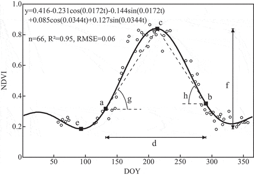
Equation (4) is an expression of the two-term Fourier function, where w is the angular frequency (w = 2π/366 ≈ 0.0172), t denotes the day of year (DOY), e_t is the random error, and β₀ through β₄ are the coefficients:

(4) $y_t={\beta }_0+{\beta }_1\cos \left(wt\right)+{\beta }_2\sin \left(wt\right)+{\beta }_3\cos \left(2wt\right)+{\beta }_{4}sin\left(2wt\right)+e_t,$(4)

According to Sun et al. (2021), β₀ measures the overall vegetation phenology, β₁ and β₂ represent general changes in vegetation phenology, and β₃ and β₄ represent minor fluctuations in vegetation phenology. In our study, the method based on the linear least-squares on GEE was used to obtain optimal fit coefficients because it can balance performance and time efficiency in tasks that need to process millions of pixels (Zhu, Woodcock, and Olofsson 2012).

Eight phenological parameters were determined from the fitted curve using a cutoff method (Table 2). The same phenological features as NDVI were extracted from the time-series data of IRECI, but different strategies were adopted when extracting the features of NDWI time-series data. This is because the time-series data of NDVI and IRECI are consistent with vegetation growth changes, whereas the NDWI of wetland vegetation tend to show a trough in summer and two peaks in spring and autumn. Therefore, some important inflection points were extracted as the time-series features of the fitted NDWI curve, including the maximum value of the function (MV) and the corresponding time (MOS); the minimum value of the function (BV) and the corresponding time (BVD); the maximum value in spring (MVL) and the corresponding time (MVLD); the maximum value in autumn (MVR) and the corresponding time (MVRD); and the seasonal amplitude (SA).

Table 2. The abbreviation and description of the eight phenological parameters.

Parameter abbreviation	Description
SOS	Start of the season: the DOY for which the left edge has increased to 20% of the seasonal amplitude measured from the left minimum level.
EOS	End of the season: the DOY for which the right edge has decreased to 20% of the seasonal amplitude measured from the right minimum level.
MOS	Medium of the season: the DOY for which the fitted function reaches the maximum value during the season.
LOS	Length of the season: the time from the start to the end of the season.
BV	Base value: the minimum value of the fitted function.
SA	Seasonal amplitude: the difference between the maximum and the base value of the fitted function.
IRS	Increase rate at the beginning of the season: the ratio of the difference between the left 20% and maximum value and the corresponding time difference.
DRS	Decrease rate at the end of the season: the absolute value of the ratio of the difference between the right 20% and maximum value and the corresponding time difference.

In addition to the VV and VH of the Sentinel-1 SAR data, SAR_sum, SAR_diff, and SAR_NDVI time-series data were constructed and composited with a median value function to extract the polarization features. The formulas used to calculate SAR_sum, SAR_diff, and SAR_NDVI are as follows:

(5) $SAR\_sum=VH+VV,$(5)

(6) $SAR\_diff=VH-VV,$(6)

(7) $SAR\_NDVI=SAR\_diff/SAR\_sum.$(7)

Due to their high similarity, a single polarization band cannot separate different wetland vegetations, but the offset between different vegetations increases under the extension of SAR_sum (Hu et al. 2021). SAR_diff may be able to reflect the biomass information of vegetation and contain smaller systematic errors. SAR_NDVI can quantitatively describe the normalized differences of different plants by imitating the method of calculating the optical NDVI. The slope is a commonly used terrain factor derived from DEM, which, in this paper, was used together with elevation for wetland plant classification. Ultimately, we extracted a total of 16 phenological features, 9 time-series features, 5 polarization features, and 2 terrain factors.

The method of analyzing features separability

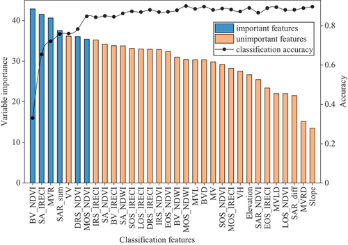
All the extracted classification features were used in the training of the RF model, but not every feature had a significant contribution to the classification accuracy. To effectively analyze the feature differences of different plant communities while reducing unnecessary tasks, we needed to select some critical features. First, the “ee.Classifier.explain()” function was called to output variable importance measures computed by the RF model on GEE. We sorted the measured results in descending order. Simply selecting top-ranked features was not advisable, as the contribution of related features was overestimated. Therefore, we sequentially input the front n (n from 1 to 32) features into the RF model for training and classification and then recorded the overall accuracy of each combination. This process was repeated five times. Then, the average overall accuracy for each scheme was calculated and plotted as a line graph. Finally, based on the results of the variable importance measures and the line graph, some important features were selected and used to analyze the separability of plant communities.

2.3.2. The methods of classification and accuracy assessment

We constructed an RF model containing 100 DTs for plant community classification. The number of variables for each split was a key parameter for the RF classifier; we set it to five, which is the square root of the number of features. To ensure that the proportion of features participating in training and validation was the same for each category, the method of stratified random sampling was used to divide all samples into two parts, of which 60% were training samples and 40% were validation samples. Then, the previously extracted features and training samples were entered into the RF model to learn classification rules and to classify different plant communities. Finally, a confusion matrix based on the validation samples was used to assess the accuracy of the classification results.

2.3.3. The methods of analyzing the spatial pattern of different wetland plant communities

Pixel-based classification results have an obvious “salt and pepper” phenomenon, showing many discrete and broken patches. To eliminate the impact of this phenomenon on the analysis of the spatial pattern, the classification results were post-processed using a series of generalization tools provided by the ArcGIS Spatial Analyst extension module. Firstly, the isolated pixels or noise were removed from the classified output using the Majority Filter tool. Then, the Boundary Clean tool was used to smooth the irregular class boundaries and clump the classes. Finally, the Region Group, Set Null, and Nibble tools were used in turn to reclassify smaller isolated pixel regions into the closest classes. The post-processed result was used to mapping the distribution of different plant communities by ArcGIS 10.2 software. In addition, we also used statistical methods to quantitatively analyze the area and proportion of different plant communities.

3. Results

3.1. Separability of plant communities characterized by different features

Figure 4 displays the variable importance measures of the RF model and the average overall accuracy of different feature combinations. The results showed that as the number of features involved in classification increased, so did the accuracy. However, after the seven features that had the highest variable importance increased the classification accuracy to 85%, the further addition of functions yielded limited improvements to accuracy. At the same time, we found that after VV participated in the classification, the accuracy did not improve compared to the previous combination. This is because SAR_sum and VV have a very strong correlation. Finally, we defined BV_NDVI, SA_IRECI, MVR, SAR_sum, DRS_NDVI, and MOS_NDVI as important features and used them to analyze the divisibility of different wetland plant communities.

Figure 4. The variable importance measures in descending order and the average overall accuracy of different feature combinations.

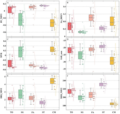
Figure 5 presents the important features distribution of wetland plant communities based on the training samples. Different wetland plant communities showed both a similarity of characteristics and obvious distinguishability. Specifically, TO and PA exhibited high similarity of features, as shown in Figure 5A&C-F, whereas the seasonal amplitude of TO (0.55 ± 0.19) characterized by IRECI was significantly lower than that of PA (1.01 ± 0.16) in Figure 5B. SG and CM could be clearly distinguished from the other three plant communities by MVR (Figure 5C), and then they could be perfectly separated by the rate of decrease at the end of the season described by NDVI (SG: 2.74 ± 0.56, CS: 4.44 ± 0.34), as shown in Figure 5E. DRS_NDVI revealed that CM had a greater rate of withering during the yellowing period than all other wetland plant communities. Additionally, ST (230.50 ± 3.50) significantly lagged behind the other communities in reaching the DOY for which the fitted function reaches the maximum value during the season characterized by NDVI, whereas CM (184.50 ± 2.50) was earlier than the other communities (Figure 5F). Through comparative analysis, it was found that the combination of SA_IRECI, MVR, and MOS_NDVI could accurately distinguish all wetland plant communities.

Figure 5. Boxplots of important features for the wetland plant communities.

TO = Typha orientalis, SG = Suaeda glauca, PA = Phragmites australis, ST = Scirpus triquater, and CM = Carex meyeriana.

3.2. Accuracy assessment of classification results

The visual verification demonstrated that the classification maps based on the RF classifier combining phenological, time-series, polarization, and terrain features reliably depicted the distribution of the plant communities in the MRWS and were proven to be highly consistent with field surveys and high-spatial-resolution images. The confusion matrix analysis indicated that the overall accuracy for the classification was 91.3%, and the Kappa coefficient was 0.90 (Table 3). To overcome the limitation of few samples and also to effectively assess the accuracy of the classification results, ten-fold cross-validation was used for accuracy evaluation. The results showed that the average overall accuracy was 88.0%, and the average Kappa coefficient was 0.87. Except for the producer’s accuracy of PA (78.3%), the user’s and producer’s accuracies of other plant communities were never smaller 80.0%, which was a satisfactory result for community-scale plant classification. The user’s and producer’s accuracies for TO were similar (~83.8%), and the omission errors were mainly derived from the PA. Although SG had a high producer’s accuracy of 92.0%, a series of commission errors from PA, Grassland, and Other resulted in a relatively low user’s accuracy of 85.2%. Benefitting from the high separability of MOS_NDVI for ST and CM, their user’s and producer’s accuracies were all very high.

Table 3. Accuracy assessment of plant community classification using the confusion matrix.

	TO	SG	PA	ST	CM	PF	WL	DF	GL	Other	UA (%)
TO	18	2	1	0	0	0	0	1	0	0	81.8
SG	0	23	1	0	0	0	0	0	2	1	85.2
PA	3	0	18	0	0	0	0	0	1	0	81.8
ST	0	0	0	23	0	0	0	0	0	0	100
CM	0	0	1	0	27	0	0	0	0	0	96.4
PF	0	0	1	0	0	25	0	1	0	0	92.6
WL	0	0	0	0	0	0	22	0	0	0	100
DF	0	0	1	0	0	1	0	23	0	0	92.0
GL	0	0	0	1	0	0	1	1	16	0	84.2
Other	0	0	0	0	0	0	0	0	1	24	96.0
PA (%)	85.7	92.0	78.3	95.8	100	96.2	95.7	88.5	80.0	96.0

TO = Typha orientalis, SG = Suaeda glauca, PA = Phragmites australis, ST = Scirpus triquater, CM = Carex meyeriana, PF = Paddy field, WL = Woodland, DF = Dry farmland, GL = Grassland, UA = user’s accuracy, and PA = producer’s accuracy. Overall accuracy = 91.3% Kappa coefficient = 0.90

3.3. Spatial pattern of different wetland plant communities

The classification map revealed the unique wetland landscape of the MRWS (Figure 6A). The total area of various natural wetland communities was 628.5 km², accounting for 42.1% of the entire MRWS (Figure 6B). There were 85.5 km² of TO community (5.7%), 182.2 km² of SG community (12.2%), 94.5 km² of PA community (6.3%), 25.2 km² of ST community (1.8%), and 241.1 km² of CM community (16.2%). Defining paddy fields and water bodies as wetlands, the total wetland area of MRWS reached 1054 km², accounting for 70.6% of the entire MRWS.

Figure 6. Classification map and area statistics of plant communities. (A) Distribution pattern of different plant communities in the MRWS. (B) Percentage of the area of different plant communities in the MRWS showed by a rose plot. (C) The distribution points of Grus leucogeranus recorded in 2020.

TO = Typha orientalis, SG = Suaeda glauca, PA = Phragmites australis, ST = Scirpus triquater, CM = Carex meyeriana, PF = Paddy field, WL = Woodland, DF = Dry farmland, GL = Grassland, and WB = Water body.

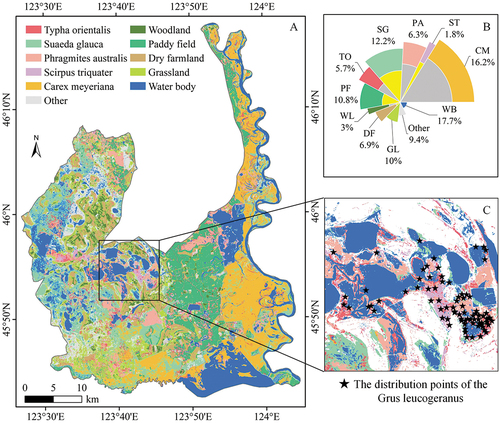
The west of the MRWS comprised large areas of typical inland salt marshes. Due to the severe land salinization, many plant communities with a certain degree of saline resistance grew in that area, such as SG, ST, PA, and TO. The Nenjiang River Basin to the east of the MRWS bred typical freshwater marsh wetlands with high peat content and low salinization degree. Numerous CM communities covered the vast floodplains. With the changes in the water level of the surface in the transition area of the water and land, the distribution of different wetland plant communities showed obvious strip-shaped characteristics. Taking Baihe Lake as an example, the main wetland plant community type gradually transitioned from TO to PA, then to ST, and then to SG with the decline in the surface water level (Figure 6C).

4. Discussion

4.1. Insights into the time-series features of different plant communities

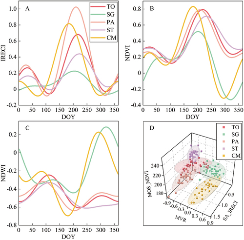
This study fully proved the capability of time-series features in classifying wetland plant communities. The two-term Fourier function was used to reconstruct the time-series curve of the representative pixels of different wetland plant communities, and significant discrepancies in phenology for different plant communities were observed (Figure 7). The IRECI time-series curve could depict the changes of plant canopy chlorophyll content and leaf area index (LAI) in a complete growth cycle (Frampton et al. 2013). Different wetland plant communities had almost the same BV, but the maximum IRECI value that they could reach was obviously different (Figure 7A). Therefore, the SA of varying plant communities was significantly different. PA had the largest SA (Figure 7A), which may be related to the greater density, higher plants, and larger LAI of the PA community. However, more water and soil information were included in the spectrum due to the lowness and sparseness of the SG and ST communities. This led to their SA being lower than that of other plant communities (Figure 7A). In addition, the SA of CM was only second to that of PA due to the unique leaf structure, and the SA of TO was smaller than that of CM (Figure 7A). Affected by the seasonal precipitation from July to September, the SG and CM communities were gradually drowned by water. As a result, they have lower NDVI (Figure 7B) and higher NDWI (Figure 7C) values at the end of the season. It was obvious that the flower and fruit period of CM (from June to July) occurred earlier than those of other plant communities, so the MOS value of CM was the smallest in the NDVI time-series curve (Figure 7B). ST had the largest MOS value (Figure 7B) because its growing period lasted until November (Xu and Tong 2018). In the three-dimensional feature space composed of SA_IRECI, MVR, and MOS_NDVI, the samples of different wetland plant communities formed five clusters, which were distributed in different areas of space (Figure 7D). This also showed that the features based on time-series data could effectively distinguish different wetland plant communities.

Figure 7. The typical time-series model of five wetland plant communities (A, B, and C) and the three-dimensional feature space of representative parameters (D).

TO = Typha orientalis, SG = Suaeda glauca, PA = Phragmites australis, ST = Scirpus triquater, CM = Carex meyeriana.

4.2. The advantages and limitations of the methods

The wetland plant community classification method proposed in this study has the following advantages: Firstly, this method integrates multi-source remote sensing images that can be obtained for free and have high resolution, including those of Sentinel-1 SAR, Sentinel-2 MSI, and DEM. This image combination is considered a more promising approach for wetland classification (Amani et al. 2019b). Secondly, the automatic classification process based on GEE makes this method extremely efficient. GEE can not only directly call various functions to deal with online remote sensing images but also upload the classification task to the cloud for rapid calculation. Finally, this method extracts multi-source characteristics, including the phenological features from the time-series data, to classify the wetland plant communities, overcoming the impact of wetland dynamicity on the classification accuracy. In addition, there are some shortcomings that need to be improved in this method. A pixel-based RF classification model, which is generally considered to have lower classification accuracy than an object-based model (Amani et al. 2019a), was used in this study. Therefore, it is recommended to explore the potential of object-based methods in wetland plant community classification in future studies. It should be noted, meanwhile, that only simple segmentation algorithms can be performed on GEE currently. To give full play to the advantages of object-based methods, it is necessary to further develop algorithms that are convenient to call by GEE. Moreover, both pixel-based and object-based methods belong to hard classification techniques, which cannot scientifically delineate the boundaries between different wetland plant communities. In contrast, probability-based fuzzy classification technology has been considered to be able to effectively solve the complex mapping problem in mixed vegetation areas (Sha et al. 2008) and is therefore suggested to be applied in future studies on MRWS wetland classification.

During the process of wetland vegetation community classification proposed in this study, the Sentinel images are free-access data sources that can be obtained for a long time worldwide, and the methods of feature extraction and classification are mature. Although the same plant community distributed at different latitudes and altitudes may have different phenological and time-series characteristics, every stage of the framework model proposed in this article is replicable. Moreover, the method could be used for classifying other vegetation types based on the selected features characterized in Sentinel images.

4.3. The enlightenment of the distribution of wetland plant communities and Grus leucogeranus to the protection of MRWS

The distribution pattern of plant communities is the result of long-term adaptation and selection of environmental conditions; it also affects the choices of migratory birds for foraging and habitats. ST is most suitable for growing in shallow-water areas with a water level below 30 cm. In the MRWS, due to the long-term water diversion of the Qianhang Station, the water level of Baihe Lake is often maintained at a high level. Therefore, the ST community is mainly distributed closer to the road by the Baihe Lake, and Grus leucogeranus is also mainly distributed here (Figure 6C). However, under the interference of pedestrians and vehicles, these areas are not conducive to the foraging and resting of Grus leucogeranus (Jiang et al. 2016). Consequently, it is necessary to dynamically adjust the water diversion strategy of Baihe Lake to increase the shallow-water area and then perform artificial supplementation of ST, thereby increasing the distribution of ST communities and providing a better habitat environment for Grus leucogeranus. The west of the MRWS is considered the most suitable habitat for Grus leucogeranus (Wang et al. 2022). Simultaneously, SG is abundant (Figure 6A), which has important ecological value such as increasing soil organic matter and reducing soil salinity. Therefore, by bolstering the monitoring of SG communities, the health of the wetland can be understood in a timely manner. Consequently, administrators can adjust wetland protection policies to prevent their further degradation and better protect Grus leucogeranus. The CM communities distributed on the floodplain of the Nenjiang River are nonrenewable natural wetlands (Wei et al. 2019), and increasing the water level fluctuation helps to increase the material yield and nutrient preservation of CM (Zhang et al. 2020). Therefore, it is necessary to formulate seasonal water resources management policies according to the growth rhythm of the CM to ensure that enough foods can be provided to waterbirds such as Otis tarda.

5. Conclusion

This study developed a novel wetland plant community classification method that extracted multi-source features from free high-resolution time-series images and performed cloud-based RF classification on GEE. This method was used in the wetland plant community classification of the MRWS using data from 2020. The results described the unique distribution pattern of different wetland plant communities with extremely high accuracy (the overall accuracy was 91.3%, and the Kappa coefficient was 0.90). This method can provide scientific decision-making support for the protection of migratory birds and plants in the MRWS, and help to improve the sustainable management measures of wetland habitats. In addition, except for sample collection, the almost fully automatic classification process gives this method strong generalization capabilities. Therefore, it is expected to play a role in large-scale and long-term wetland plant community classification.

Authors responsibilities

K. Feng designed the classification program and wrote this article. The concept of this research was initially developed by D. Mao, and he guided the writing and modification of the article. Z. Qiu and Y. Zhao participated in code writing and chart production. Z. Wang supervised the whole process.

Acknowledgements

First of all, I am very grateful to Google Earth Engine (https://earthengine.google.com/) for providing free services. I would like to thank Mr. Yu An for his help in the field survey. I also want to thank my parents for their full support and encouragement to me. Finally, we sincerely thank the editor and reviewers for their time and effort in providing detailed comments that helped improve the quality of this paper.

Disclosure statement

The authors declare that they have no known competing financial interests or personal relationships that could have appeared to influence the work reported in this paper.

Data availability statement

The data, models, or codes generated or used in this paper are available from Google Earth Engine upon reasonable request.

Correction Statement

This article has been corrected with minor changes. These changes do not impact the academic content of the article.

Additional information

Funding

This research was jointly funded by the National Natural Science Foundation of China [42222103, 42171379, and 42101379], the Science and Technology Development Program of Jilin Province, China [20210101396JC and 20200301014RQ], the Youth Innovation Promotion Association of Chinese Academy of Sciences [2017277 and 2021227], the Professional Association of the Alliance of International Science Organizations [ANSO-PA-2020-14], and the Young Scientist Group Project of Northeast Institute of Geography and Agroecology, Chinese Academy of Sciences [2022QNXZ03].

References

- Amani, M., B. Brisco, M. Afshar, S. M. Mirmazloumi, S. Mahdavi, S. M. J. Mirzadeh, W. Huang, and J. Granger. 2019a. “A Generalized Supervised Classification Scheme to Produce Provincial Wetland Inventory Maps: An Application of Google Earth Engine for Big Geo Data Processing.” Big Earth Data 3 (4): 378–394. doi:10.1080/20964471.2019.1690404.
- Amani, M., S. Mahdavi, M. Afshar, B. Brisco, W. Huang, S. M. J. Mirzadeh, L. White, S. Banks, J. Montgomery, and C. Hopkinson. 2019b. “Canadian Wetland Inventory Using Google Earth Engine: The First Map and Preliminary Results.” Remote Sensing 11 (7): 842. doi:10.3390/rs11070842.
- Belluco, E., M. Camuffo, S. Ferrari, L. Modenese, S. Silvestri, A. Marani, and M. Marani. 2006. “Mapping Salt-Marsh Vegetation by Multispectral and Hyperspectral Remote Sensing.” Remote Sensing of Environment 105 (1): 54–67. doi:10.1016/j.rse.2006.06.006.
- Chen, B., X. Xiao, X. Li, L. Pan, R. Doughty, J. Ma, J. Dong, et al. 2017. “A Mangrove Forest Map of China in 2015: Analysis of Time Series Landsat 7/8 and Sentinel-1A Imagery in Google Earth Engine Cloud Computing Platform.” ISPRS Journal of Photogrammetry and Remote Sensing 131:104–120. doi:10.1016/j.isprsjprs.2017.07.011
- Correll, M. D., W. Hantson, T. P. Hodgman, B. B. Cline, C. S. Elphick, W. G. Shriver, E. L. Tymkiw, and B. J. Olsen. 2019. “Fine-Scale Mapping of Coastal Plant Communities in the Northeastern USA.” Wetlands 39 (1): 17–28. doi:10.1007/s13157-018-1028-3.
- Dong, D., C. Wang, J. Yan, Q. He, J. Zeng, and Z. Wei. 2020. “Combing Sentinel-1 and Sentinel-2 Image Time Series for Invasive Spartina Alterniflora Mapping on Google Earth Engine: A Case Study in Zhangjiang Estuary.” Journal of Applied Remote Sensing 14 (4): 044504. doi:10.1117/1.JRS.14.044504.
- Dronova, I. 2015. “Object-Based Image Analysis in Wetland Research: A Review.” Remote Sensing 7 (5): 6380–6413. doi:10.3390/rs70506380.
- Du, B., D. Mao, Z. Wang, Z. Qiu, H. Yan, K. Feng, and Z. Zhang. 2021. “Mapping Wetland Plant Communities Using Unmanned Aerial Vehicle Hyperspectral Imagery by Comparing Object/Pixel-Based Classifications Combining Multiple Machine-Learning Algorithms.” IEEE Journal of Selected Topics in Applied Earth Observations and Remote Sensing 14: 8249–8258. doi:10.1109/JSTARS.2021.3100923.
- Frampton, W. J., J. Dash, G. Watmough, and E. J. Milton. 2013. “Evaluating the Capabilities of Sentinel-2 for Quantitative Estimation of Biophysical Variables in Vegetation.” ISPRS Journal of Photogrammetry and Remote Sensing 82: 83–92. doi:10.1016/j.isprsjprs.2013.04.007.
- Gorelick, N., M. Hancher, M. Dixon, S. Ilyushchenko, D. Thau, and R. Moore. 2017. “Google Earth Engine: Planetary-Scale Geospatial Analysis for Everyone.” Remote Sensing of Environment 202: 18–27. doi:10.1016/j.rse.2017.06.031.
- Granero-Belinchon, C., K. Adeline, A. Lemonsu, and X. Briottet. 2020. “Phenological Dynamics Characterization of Alignment Trees with Sentinel-2 Imagery: A Vegetation Indices Time Series Reconstruction Methodology Adapted to Urban Areas.” Remote Sensing 12 (4): 639. doi:10.3390/rs12040639.
- He, C., Y. Song, H. Lang, H. Li, and X. Sun. 2002. “Migratory Dynamics of Siberian Crane and Environmental Conditions at Its Stop-over Site.” Biodiversity Science 10 (3): 286–290. doi:10.17520/biods.2002039.
- Henderson, F. M., and A. J. Lewis. 2008. “Radar Detection of Wetland Ecosystems: A Review.” International Journal of Remote Sensing 29 (20): 5809–5835. doi:10.1080/01431160801958405.
- Hladik, C., J. Schalles, and M. Alber. 2013. “Salt Marsh Elevation and Habitat Mapping Using Hyperspectral and LIDAR Data.” Remote Sensing of Environment 139: 318–330. doi:10.1016/j.rse.2013.08.003.
- Hu, Y., B. Tian, L. Yuan, X. Li, Y. Huang, R. Shi, X. Jiang, L. Wang, and C. Sun. 2021. “Mapping Coastal Salt Marshes in China Using Time Series of Sentinel-1 SAR.” ISPRS Journal of Photogrammetry and Remote Sensing 173: 122–134. doi:10.1016/j.isprsjprs.2021.01.003.
- Jiang, H., Y. Wen, L. Zou, Z. Wang, C. He, and C. Zou. 2016. “The Effects of a Wetland Restoration Project on the Siberian Crane (Grus Leucogeranus) Population and Stopover Habitat in Momoge National Nature Reserve, China.” Ecological Engineering 96: 170–177. doi:10.1016/j.ecoleng.2016.01.016.
- Kloiber, S. M., R. D. Macleod, A. J. Smith, J. F. Knight, and B. J. Huberty. 2015. “A Semi-Automated, Multi-Source Data Fusion Update of A Wetland Inventory for East-Central Minnesota, USA.” Wetlands 35 (2): 335–348. doi:10.1007/s13157-014-0621-3.
- Kumar, L., and P. Sinha. 2014. “Mapping Salt-Marsh Land-Cover Vegetation Using High-Spatial and Hyperspectral Satellite Data to Assist Wetland Inventory.” GIScience & Remote Sensing 51 (5): 483–497. doi:10.1080/15481603.2014.947838.
- Li, J., and W. Chen. 2005. “A Rule-Based Method for Mapping Canada’s Wetlands Using Optical, Radar and DEM Data.” International Journal of Remote Sensing 26 (22): 5051–5069. doi:10.1080/01431160500166516.
- Li, J., W. Chen, and R. Touzi. 2007. “Optimum RADARSAT-1 Configurations for Wetlands Discrimination: A Case Study of the Mer Bleue Peat Bog.” Canadian Journal of Remote Sensing 33 (sup1): S46–S55. doi:10.5589/m07-046.
- Liu, D., H. Liu, H. Zhang, M. Cao, Y. Sun, W. Wu, and C. Lu. 2016. “Potential Natural Exposure of Endangered Red-Crowned Crane (Grus Japonensis) to Mycotoxins Aflatoxin B1, Deoxynivalenol, Zearalenone, T-2 Toxin, and Ochratoxin A.” Journal of Zhejiang University-SCIENCE B 17 (2): 158–168. doi:10.1631/jzus.B1500211.
- Luo, J., H. Duan, R. Ma, X. Jin, F. Li, W. Hu, K. Shi, and W. Huang. 2017. “Mapping Species of Submerged Aquatic Vegetation with Multi-Seasonal Satellite Images and considering Life History Information.” International Journal of Applied Earth Observation and Geoinformation 57 (May): 154–165. doi:10.1016/j.jag.2016.11.007.
- Mahdavi, S., B. Salehi, J. Granger, M. Amani, B. Brisco, and W. Huang. 2018. “Remote Sensing for Wetland Classification: A Comprehensive Review.” GIScience & Remote Sensing 55 (5): 623–658. doi:10.1080/15481603.2017.1419602.
- Mahdianpari, M., H. Jafarzadeh, J. E. Granger, F. Mohammadimanesh, B. Brisco, B. Salehi, S. Homayouni, and Q. Weng. 2020. “A Large-Scale Change Monitoring of Wetlands Using Time Series Landsat Imagery on Google Earth Engine: A Case Study in Newfoundland.” GIScience & Remote Sensing 57 (8): 1102–1124. doi:10.1080/15481603.2020.1846948.
- Mahdianpari, M., B. Salehi, F. Mohammadimanesh, S. Homayouni, and E. Gill. 2018. “The First Wetland Inventory Map of Newfoundland at a Spatial Resolution of 10 M Using Sentinel-1 and Sentinel-2 Data on the Google Earth Engine Cloud Computing Platform.” Remote Sensing 11 (1): 43. doi:10.3390/rs11010043.
- Mahdianpari, M., B. Salehi, F. Mohammadimanesh, and M. Motagh. 2017. “Random Forest Wetland Classification Using ALOS-2 L-Band, RADARSAT-2 C-Band, and TerraSAR-X Imagery.” ISPRS Journal of Photogrammetry and Remote Sensing 130: 13–31. doi:10.1016/j.isprsjprs.2017.05.010.
- Mao, D., L. Luo, Z. Wang, M. C. Wilson, Y. Zeng, B. Wu, and J. Wu. 2018. “Conversions between Natural Wetlands and Farmland in China: A Multiscale Geospatial Analysis.” Science of the Total Environment 634: 550–560. doi:10.1016/j.scitotenv.2018.04.009.
- Mao, D., Z. Wang, B. Du, L. Li, Y. Tian, M. Jia, Y. Zeng, K. Song, M. Jiang, and Y. Wang. 2020. “National Wetland Mapping in China_ A New Product Resulting from Object-Based and Hierarchical Classification of Landsat 8 OLI Images.” ISPRS Journal of Photogrammetry and Remote Sensing 164: 11–25. doi:10.1016/j.isprsjprs.2020.03.020.
- Mao, D., H. Yang, Z. Wang, K. Song, J. R. Thompson, and R. J. Flower. 2022. “Reverse the Hidden Loss of China’s Wetlands.” Science 376 (6597): 1061. doi:10.1126/science.adc8833.
- Martínez-López, J., M. F. Carreño, J. A. Palazón-Ferrando, J. Martínez-Fernández, and M. A. Esteve. 2014. “Remote Sensing of Plant Communities as a Tool for Assessing the Condition of Semiarid Mediterranean Saline Wetlands in Agricultural Catchments.” International Journal of Applied Earth Observation and Geoinformation 26: 193–204. doi:10.1016/j.jag.2013.07.005.
- Mitsch, W. J. 1996. “Managing the World’s Wetlands — Preserving and Enhancing Their Ecological Functions.” Internationale Vereinigung Für Theoretische Und Angewandte Limnologie: Verhandlungen 26 (1): 139–147. doi:10.1080/03680770.1995.11900698.
- Pengra, B. W., C. A. Johnston, and T. R. Loveland. 2007. “Mapping an Invasive Plant, Phragmites Australis, in Coastal Wetlands Using the EO-1 Hyperion Hyperspectral Sensor.” Remote Sensing of Environment 108 (1): 74–81. doi:10.1016/j.rse.2006.11.002.
- Petus, C., M. Lewis, and D. White. 2013. “Monitoring Temporal Dynamics of Great Artesian Basin Wetland Vegetation, Australia, Using MODIS NDVI.” Ecological Indicators 34 (November): 41–52. doi:10.1016/j.ecolind.2013.04.009.
- Rapinel, S., C. Mony, L. Lecoq, B. Clément, A. Thomas, and L. Hubert-Moy. 2019. “Evaluation of Sentinel-2 Time-Series for Mapping Floodplain Grassland Plant Communities.” Remote Sensing of Environment 223: 115–129. doi:10.1016/j.rse.2019.01.018.
- Rodwell, J. S., D. Evans, and J. H. J. Schaminée. 2018. “Phytosociological Relationships in European Union Policy-Related Habitat Classifications.” Rendiconti Lincei. Scienze Fisiche e Naturali 29 (2): 237–249. doi:10.1007/s12210-018-0690-y.
- Rummell, A. J., J. X. Leon, H. P. Borland, B. B. Elliott, B. L. Gilby, C. J. Henderson, and A. D. Olds. 2022. “Watching the Saltmarsh Grow: A High-Resolution Remote Sensing Approach to Quantify the Effects of Wetland Restoration.” Remote Sensing 14 (18): 4559. doi:10.3390/rs14184559.
- Sanchez-Hernandez, C., D. S. Boyd, and G. M. Foody. 2007. “Mapping Specific Habitats from Remotely Sensed Imagery: Support Vector Machine and Support Vector Data Description Based Classification of Coastal Saltmarsh Habitats.” Ecological Informatics 2 (2): 83–88. doi:10.1016/j.ecoinf.2007.04.003.
- Schmidt, K. S., and A. K. Skidmore. 2003. “Spectral Discrimination of Vegetation Types in a Coastal Wetland.” Remote Sensing of Environment 85 (1): 92–108. doi:10.1016/S0034-4257(02)00196-7.
- Sha, Z., Y. Bai, Y. Xie, M. Yu, and L. Zhang. 2008. “Using a Hybrid Fuzzy Classifier (HFC) to Map Typical Grassland Vegetation in Xilin River Basin, Inner Mongolia, China.” International Journal of Remote Sensing 29 (8): 2317–2337. doi:10.1080/01431160701408436.
- Sun, C., J. Li, L. Cao, Y. Liu, S. Jin, and B. Zhao. 2020. “Evaluation of Vegetation Index-Based Curve Fitting Models for Accurate Classification of Salt Marsh Vegetation Using Sentinel-2 Time-Series.” Sensors 20 (19): 5551. doi:10.3390/s20195551.
- Sun, C., J. Li, Y. Liu, Y. Liu, and R. Liu. 2021. “Plant Species Classification in Salt Marshes Using Phenological Parameters Derived from Sentinel-2 Pixel-Differential Time-Series.” Remote Sensing of Environment 256: 112320. doi:10.1016/j.rse.2021.112320.
- Wang, G., C. Wang, Z. Guo, L. Dai, Y. Wu, H. Liu, Y. Li, et al. 2020. “A Multiscale Approach to Identifying Spatiotemporal Pattern of Habitat Selection for Red-Crowned Cranes.” Science of the Total Environment 739:139980. doi:10.1016/j.scitotenv.2020.139980
- Wang, M., D. Mao, X. Xiao, K. Song, M. Jia, C. Ren, and Z. Wang. 2023. “Interannual Changes of Coastal Aquaculture Ponds in China at 10-m Spatial Resolution during 2016–2021.” Remote Sensing of Environment 284 (January): 113347. doi:10.1016/j.rse.2022.113347.
- Wang, Y., M. Gong, C. Zou, T. Zhou, W. Wen, G. Liu, H. Li, and W. Tao. 2022. “Habitat Selection by Siberian Cranes at Their Core Stopover Area during Migration in Northeast China.” Global Ecology and Conservation 33: e01993. doi:10.1016/j.gecco.2021.e01993.
- Wei, J., J. Gao, N. Wang, Y. Liu, Y. Wang, Z. Bai, X. Zhuang, and G. Zhuang. 2019. “Differences in Soil Microbial Response to Anthropogenic Disturbances in Sanjiang and Momoge Wetlands, China.” FEMS Microbiology Ecology 95 (8): fiz110. doi:10.1093/femsec/fiz110.
- Wen, D., Y. Hu, Z. Xiong, Y. Chang, Y. Li, Y. Wang, M. Liu, and J. Zhu. 2020. “Potential Suitable Habitat Distribution and Conservation Strategy for the Siberian Crane (Grus Leucogeranus) at Spring Stopover Sites in Northeastern China.” Polish Journal of Environmental Studies 29 (5): 3375–3384. doi:10.15244/pjoes/113453.
- Xu, Y., and C. Tong. 2018. “Biomass Allocation Characteristics of Scirpus Mariqueter and Corresponding Influencing Factors in Jiuduansha Shoals of the Yangtze Estuary.” Acta Ecologica Sinica 38 (19): 7034–7044. doi:10.5846/stxb201710241903.
- Yang, G., K. Huang, W. Sun, X. Meng, D. Mao, and Y. Ge. 2022. “Enhanced Mangrove Vegetation Index Based on Hyperspectral Images for Mapping Mangrove.” ISPRS Journal of Photogrammetry and Remote Sensing 189 (July): 236–254. doi:10.1016/j.isprsjprs.2022.05.003.
- Zhang, D., M. Zhang, S. Tong, Q. Qi, X. Wang, and X. Lu. 2020. “Growth and Physiological Responses of Carex Schmidtii to Water-Level Fluctuation.” Hydrobiologia 847 (3): 967–981. doi:10.1007/s10750-019-04159-z.
- Zhang, Y., D. Lu, B. Yang, C. Sun, and M. Sun. 2011. “Coastal Wetland Vegetation Classification with a Landsat Thematic Mapper Image.” International Journal of Remote Sensing 32 (2): 545–561. doi:10.1080/01431160903475241.
- Zhou, Q., Y. Ke, X. Wang, J. Bai, D. Zhou, and X. Li. 2022. “Developing Seagrass Index for Long Term Monitoring of Zostera Japonica Seagrass Bed: A Case Study in Yellow River Delta, China.” ISPRS Journal of Photogrammetry and Remote Sensing 194 (December): 286–301. doi:10.1016/j.isprsjprs.2022.10.011.
- Zhu, Z., C. E. Woodcock, and P. Olofsson. 2012. “Continuous Monitoring of Forest Disturbance Using All Available Landsat Imagery.” Remote Sensing of Environment 122: 75–91. doi:10.1016/j.rse.2011.10.030.