Evaluating the contribution of Sentinel-2 view and illumination geometry to the accuracy of retrieving essential crop parameters

ABSTRACT

Wide field-of-view (FOV) sensors such as Sentinel-2 exhibit per-pixel view and illumination geometry variation that may influence the retrieval accuracy of essential crop biophysical and biochemical variables (BVs) for precision agriculture. However, this aspect is rarely studied in the existing literature. Hence, the current study aimed to evaluate the contribution of view and illumination geometries to the accuracy of retrieving Leaf Chlorophyll a and b (LC_ab), Canopy Chlorophyll Content (CCC), and Leaf Area Index (LAI) using the Random Forest (RF). The experiments were performed on various input variable scenarios where per-pixel geometric covariates, i.e. View and Sun Zenith Angles (VZA and SZA, respectively), and Relative Azimuth Angle (RAA), are excluded and included in spectral bands (SB) and spectral vegetation indices (SVIs), respectively, in two semi-arid areas. The results showed that spectral bands or vegetation indices combined with geometric covariates improved the R² by 10–15% for LAI and 3–5% for CCC. In contrast, negligible improvements of 1–2% were achieved for LC_ab with cross-validation test data and independent held-out dataset, respectively. In agreement with previous studies, VZA and SZA were among the topmost influential variables in the RF models for estimating LAI, LC_ab, and CCC. Collectively, per-pixel geometric variables explained more than 30% of the variability in surface reflectance for all Sentinel-2 spectral bands (p < 2.2e-16). Overall, the results showed that incorporating geometric covariates improved the accuracy of retrieving BVs; thus, it provided additional information that improves the predictive power of SB and SVIs. The significant benefits of the geometric variables were mainly realized for canopy-level BVs (i.e. LAI and CCC) than for LC_ab. Therefore, it is recommended to incorporate per-pixel view and illumination geometry in estimating LAI and CCC, especially when using wide-view sensors such as Sentinel-2. However, further testing in different phenology, site and acquisition conditions is needed to confirm the contribution of the geometric covariates to facilitate reliable retrieval of BVs from remotely sensed data and aid better agronomic decisions.

KEYWORDS:

• Chlorophyll Content
• Leaf Area Index
• Sentinel-2
• Random Forest
• red-edge vegetation indices
• sun-sensor geometry

1. Introduction

Improving the estimation of crop biophysical and biochemical variables (BVs) is critical to support agricultural management practices, aid the optimization of farm inputs, and monitor agricultural production at landscape to regional level (Alexandridis, Ovakoglou, and Clevers 2020). Plant parameters such as the Leaf Chlorophyll a and b (LC_ab), Leaf Area Index (LAI), and Canopy Chlorophyll Content (CCC) are often used in as input to models monitoring the physiological status of plants and their health (Lu et al. 2018). The LAI is considered an essential parameter for quantitatively analyzing a series of biophysical processes which describe vegetation dynamics (Alexandridis, Ovakoglou, and Clevers 2020; Liu et al. 2017). LC_ab and CCC, on the other hand, are critical for characterizing the photosynthetic activity of crops. Because they are both related to Nitrogen (N) content (Clevers, Kooistra, and Van den Brande 2017), CCC and LC_ab are critical agronomic parameters to monitor N content at canopy and leaf scales. Moreover, the photosynthetic activities of crops hinge on water availability. Thus, crop stress caused by declining soil moisture can be detected rapidly by assessing the changes in chlorophyll content.

LAI and LC_ab are traditionally measured using destructive and lab-based methods (Liang et al. 2011), which entail prohibitive operational costs for vast areal and temporal coverages. Therefore, optical handheld LAI instruments, such as Accu-Par Ceptometer, digital hemispherical photography, SunScan, and LAI-2200C and chlorophyll meters such as MC-100 Chlorophyll Concentration Meter and SPAD-502, provide reasonably accurate measurements of effective LAI and LC_ab in a rapid and noninvasive manner. When coupled with satellite-based remotely sensed data, the detailed retrieval of crop BVs can be realized over vast areas at frequent intervals, thus suitable for precision agriculture needs.

For years, spectral vegetation indices (SVIs) have shaped the scientific advancements in the retrieval of BVs due to their high correlation with vegetation traits such as leaf pigments, nitrogen, and LAI (Lee et al. 2008; Clevers and Gitelson 2013; Clevers, Kooistra, and Van den Brande 2017; Haboudane et al. 2008). Such SVIs were developed using visible and near-infrared (VNIR) bands from earlier missions such as AVHRR (Advanced Very High-Resolution Radiometer), MODIS (Moderate Resolution Imaging Spectroradiometer), and Landsat. Hence, SVIs such as the NDVI (ROUSE 1973) and its variants – designed to overcome background effects, atmospheric interference, and saturation – are popular in agronomic and other vegetation applications. However, VNIR indices are known to suffer from underestimations at various (i.e. low or high) biomass, chlorophyll content and LAI. Recently, red-edge SVIs based on quasi-hyperspectral sensors, such as Worldview-2 and Multi-Spectral Instrument (MSI) on board Sentinel-2, were shown to enhance the accuracy of BVs and overcome challenges of VIS/NIR indices (Delegido et al., 2013; Dimitrov et al., 2019; Fitzgerald et al., 2010; Sibanda et al., 2019). Other studies have demonstrated the potential of Radiative Transfer Models (RTMs) (Jacquemoud et al. 2009). However, such models are beset with errors resulting from poor parameterization and complexity, which may result in considerable uncertainty in the retrieved BVs (Xu et al. 2019; Durbha, King, and Younan 2007).

Alternatively, MLRAs (Machine Learning Regression Algorithms) were tailored to learn complex relationships between measured BVs and reflectance data from satellite imagery (Karimi et al. 2018; Mao et al. 2019). The application of MLRAs for the retrieval of important crop BVs is considered ideal due to their high accuracy and flexibility to process multiple features and datasets (Apolo-Apolo et al., 2020). It is, therefore, essential to examine whether such approaches could improve future product development, aid informed agricultural management decisions, and accelerate precision agriculture, especially in developing regions such as Africa where operational use of Earth observation for precision agriculture is still in its infancy.

Vegetation canopy reflectance is affected by the biophysical and biochemical traits, phenological and environmental changes, signal attenuation by the atmosphere, topographic effects, and acquisition conditions, among others (Ollinger 2011). In particular, satellite-based radiometric measurements exhibit non-negligible effects from view and illumination geometry or Bidirectional Reflectance Distribution Function (BRDF) that may introduce ambiguity in retrieving BVs. BRDF refers to the ratio of the solar incident irradiance $E_i$ from a given direction on a target surface to its contribution to the reflected radiance $L_r$ from the same surface in another direction. Mathematically, it is expressed as $f_r\left({\theta }_i,{\varphi }_i;{\theta }_r,{\varphi }_r\right)=\frac{d{L}_r\left({\theta }_i,{\varphi }_i;{\theta }_r,{\varphi }_r;E_i\right)}{d{E}_i\left({\theta }_i,{\varphi }_i\right)}\left[s{r}^{-1}\right]$, where $\theta$ and $\varphi$ indicate a direction, $i$ and $r$ are the quantities associated with the incident and reflected radiant flux, respectively. $E_i$, $L_r$, and $d$ denote the incident irradiance, reflected radiance, and differential quantity, respectively (Nicodemus et al. 1977). Essentially, the BRDF refers to the surface reflectance variation with the varying view and illumination geometry (Nagol et al. 2015). Due to the different acquisition angles between sensors and orbits and the sun-angle variations across different seasons, latitudes, and terrains, previous studies dedicated considerable effort to reducing BRDF effects (Roy et al. 2017b; Roy, Li, and Zhang 2017a). The reduction of BRDF effects is particularly essential for obtaining temporally consistent data across different sensors to enhance the accuracy and temporal consistency of land cover maps (Nagol et al. 2015), canopy structural parameters (Sharma, Kajiwara, and Honda 2013), and BVs (Pocewicz et al. 2007).

In that regard, techniques such as the c-factor (Roy et al. 2017b; Roy, Li, and Zhang 2017a) – based on a semi-empirical Ross Thick/Li Sparse-Reciprocal BRDF model (Schaaf et al. 2002) – and integrated topographic and angular normalization (Yin et al. 2020)—based on the C-factor and Path Length Correction (PLC)—have been proposed for Landsat and Sentinel-2. Other techniques, such as the MODIS BRDF/Albedo algorithm, have been used to produce Nadir BRDF-Adjusted surface Reflectance (NBAR) for decades (Schaaf et al. 2002). For high-resolution sensors, e.g. Sentinel-2, atmospheric correction tools such as Sen2Cor provide an option to perform empirical BRDF corrections (Louis et al. 2016). However, the BRDF correction option is often left deactivated in validation studies to be consistent with other methods (Sola et al. 2018). So far, the radiometric variation introduced by the sensor view and illumination geometry has been regarded as a nuisance. However, such geometry-induced spectral variation may provide additional structural information content due to the dependence of reflected radiance on the geometric configurations (Kneubühler et al. 2008). This is especially highlighted by the studies utilizing multi-angular data (Verrelst et al. 2008; Duveiller, Lopez-Lozano, and Cescatti 2015; Vierling, Deering, and Eck 1997), showing its utility for characterizing structural variation of various layers of vegetation (e.g. foliage clumping) that affects LAI. However, high-resolution multi-angular data are costly and can only be acquired by commercial satellites (Roosjen et al. 2018). Other studies showed that view and illumination geometry have a considerable effect on vegetation indices and phenology metrics (Ranson, Daughtry, and Biehl 1986; Middleton 1991; Pocewicz et al. 2007; Verrelst et al. 2008; Ma et al. 2020).

Meanwhile, studies (Nagol et al. 2015; Roy et al. 2017b) also show that popular multispectral sensors (e.g. Landsat and Sentinel-2) exhibit within-scene angular effects. In particular, Sentinel-2’s wide Field-of-View (FOV), i.e. ~20.6° (~295 km), has been shown to exhibit considerable within-scene surface anisotropy due to varying per-pixel view and illumination geometry for each of its 12 detectors (Gascon et al. 2017; Roy et al. 2017b). Fortunately, Sentinel-2 data provides a pixel-wise and band-wise view and illumination geometry, thus providing some prospects to address the questions such as (1) How much variability in crop canopy reflectance is explained by the view and illumination geometry variations? (2) What is the contribution of incorporating per-pixel view and illumination geometry to the accuracy of retrieving crop BVs using MLRAs? (3) Are geometric variables influential in improving modeling accuracy when coupled with commonly used radiometric input variables, i.e. spectral bands and SVIs? These will clarify whether acquisition conditions (i.e. sun-view geometry) provide additional information or noise to the estimation of crop BVs. The operational Sentinel-2 Land bio-physical processor (SL2P) (available in Sentinel Application Platform, SNAP), based on pretrained ANN, uses per-pixel geometric information as input to the biophysical retrieval process (Weiss and Baret 2020). However, such complex, “black-box” (or opaque) models do not provide model agnostics, which would otherwise reveal the influence of per-pixel geometric variables on the estimations. Interpretable MLRAs such as RF are essential for obtaining new causal links and novel insights between predictor and response variables. Moreover, they enable the detection and diagnosis of biases in the MLRA models and associated input data, hence essential for improved satellite-based value-added products (Azodi et al., 2020).

In that context, this study evaluated the contribution of view and illumination geometries on crop biophysical and biochemical retrieval using the Random Forest (RF) regression algorithm and various combinations of Sentinel-2 covariates. The evaluated covariates consisted of spectral bands (SB), spectral vegetation indices (SVIs), SB combined with sensor view-illumination geometries (SB + Angles), and SVIs combined with sensor view and illumination geometries (SVIs + Angles), and all variables (Avar). The specific objectives were threefold: (1) To quantify the amount of spectral variability caused by the per-pixel view and illumination geometry in Sentinel-2 spectral bands; (2) To determine the contribution of per-pixel view and illumination geometry to the accuracy of retrieving LAI, LC_ab and CCC with RF; and (3) To identify the most important (i.e. influential) variables contributing to the model accuracy, considering different combinations of covariates. The study area is comprised of two semi-arid African agricultural sites, located in South Africa.

2. Study area

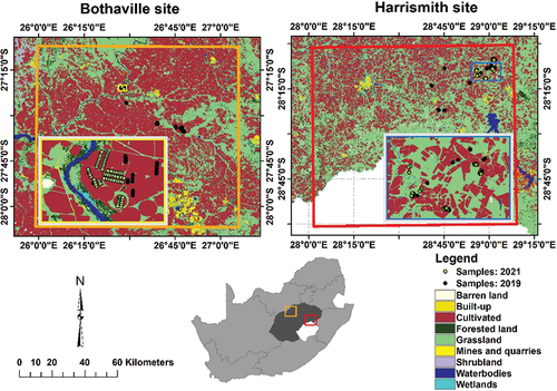
Bothaville and Harrismith sites are located in the Free State province, South Africa (see Figure 1). The sites are characterized by mainly commercial farming of crops and livestock takes place. The summer growing season, which constitutes most cropping activities in both sites, has mean annual temperatures of about 18°C and 19.2°C and mean annual rainfall of about 584 and 115 mm, respectively (Kganyago et al. 2020, 2020). The crops in the sites are generally similar, i.e. predominantly maize and beans, while sunflower and groundnuts are dominant in Bothaville only. Cropping takes place on flat slopes with sandy-loamy and sandy soils in Bothaville and undulating slopes with clay-loamy soils in Harrismith. The summer cropping calendar at both sites is from December to May or June.

Figure 1. Land cover distributions in Bothaville and Harrismith (orange and red squares), Free State province (dark grey), South Africa (adopted from Kganyago 2022). The insert maps are projected to UTM (Universal Transverse Mercator) with WGS-84 (World geodetic System 1984) Datum. The land cover dataset was obtained from the Department of Forestry, Fisheries and the Environment (https://egis.environment.gov.za/gis_data_downloads, accessed 20 March 2021).

3. Materials and methods

The summary of the methods followed in this study is given in Figure 2.

Figure 2. The schematic representation of the methods used in this study. Five experimental scenarios, i.e. Spectral bands (SB), SB and Angles (SB + Angles), Spectral vegetation indices (SVIs), SVIs and Angles (SVIs + Angles), and All variables (Avar) were used for crop biophysical and biochemical variable (BV) retrieval using two test datasets, i.e. cross-validation test dataset and an independent held-out test (i.e. unseen) dataset.

3.1. Data

3.1.1. In situ data

LAI and LC_ab in situ data were collected nondestructively in Harrismith and Bothaville between 15 and 26 March 2021 and between 11 and 23 April 2021, respectively. Similar sampling strategy was followed at the two sites, where the plots (each with 40 m × 40 m) were designed along transects chosen randomly within various crop fields. Six to eight random measurements were captured within each plot and averaged. Each plot’s centroids were Geo-tagged with a GPS coordinate and a picture using TDC600 handheld Data Collector (Trimble® Inc., Westminster, CO, USA) with 1.5 m GNSS accuracy. Plant Canopy Analyzer 2200c (Li-Cor, Inc., Lincoln, NE, USA), equipped with an 180° field-of-view (FOV) view cap, was used to measure LAI. The view cap ensured that any possible uncertainty caused by the operator’s influence and uneven sky conditions are avoided. On the other hand, MC-100 (Apogee Instruments, Inc., Logan, UT, USA) was used to acquire LC_ab measurements on sun-exposed leaves. The CCC was obtained as a product of plot-averaged LC_ab and LAI measurements (LC_ab × LAI) (Jacquemoud et al. 2009). Because our aim was to develop generic models, we combined the in situ data from each site, i.e. beans, maize, and peanuts and beans and maize found in Bothaville and Harrismith, respectively. Our approach is aligned with NGUY-Robertson et al. (2012) who note that crop types with different physiological pathways (i.e. C3 and C4), plant structures and architectures are representative many other crop types’ physiological and anatomical traits. Therefore, the developed models are likely widely applicable to multiple crops, critical for sub-Saharan Africa, where inter-cropping agricultural practices dominate.

3.1.2. Sentinel-2 data

Sentinel-2 Multi-Spectral Imager (MSI) images (granule: 35JMK and 35JPJ), acquired on 20 21 March 2022T07:46:11.024Z and 20 21 April 2014T07:56:01.024Z, over Harrismith (Sensing orbit number: 135) and Bothaville (Sensing orbit number: 35), respectively, were retrieved from Sentinel Hub (Sinergise Laboratory for geographical information systems, Ltd., Ljubljana, Slovenia) at processing Level-2A, i.e. surface reflectance. Sentinel-2A and 2B have the identical MSI sensors and provide a 5-day revisit period. The images used here were acquired by Sentinel-2A satellite in a descending orbit direction. Out of the 13 MSI spectral bands, which are provided in various spatial resolutions, we used only the 10 m and 20 m spectral bands which are designed for land applications: 490 nm (B2: blue), 560 nm (B3: green), 665 nm (B4: red), 705 nm (B5: red-edge), 740 nm (B6: red-edge), 783 nm (B7: red-edge), 865 nm (B8A: NIR), 842 nm (B8: NIR), 1610 nm (B11: SWIR-1), and 2190 nm (B11: SWIR-2). The details of the Sentinel-2 calibration are reported by Gascon et al. (2017). In addition to radiometric data, each tile, i.e. 100 km × 100 km, is packaged within various folders containing the ancillary, spectral data and band-wise and mean per-pixel view and illumination geometry, i.e. View and Sun Zenith Angle (VZA and SZA, respectively), View and Sun Azimuth Angle (VAA and SAA, respectively) on a 5-km grid (Gascon et al. 2017). The mean SZA, mean VZA, mean SAA, and mean VAA and spectral bands acquired by different detectors were resampled to a standard spatial resolution, i.e. 20 m, using the bilinear resampling technique.

Other land covers, i.e. other than croplands, were removed from the images by applying a crop mask generated from the National Crop Boundaries data (Cropestimatesconsortium 2017). To limit the analyses to the active croplands of 2021 summer growing season, we applied an NDVI-based vegetation mask, where non-vegetated pixels were considered as those with NDVI <0.2.

3.2. Multiple linear regression

As shown in Figure 3, the SZA, VZA, and RAA vary spatially within a single Sentinel-2 MSI tile. Gascon et al. (2017) indicate that Sentinel-2 acquisition geometries differ according to the 12 detectors for each spectral band due to the sensor’s push-broom design. This spatial variability is clear in Figures 3 and 4, where it is evident that the SZA, VZA, and RAA vary by pixel across the scene. Therefore, it is also expected that pixel-wise surface reflectance over crops would vary by sensor view and illumination geometry (Verrelst et al. 2008; Jay et al. 2017; Galvao et al. 2011; Biriukova et al. 2020).

Figure 3. Spatial (per-pixel) variation of Sentinel-2 illumination and view angles over the two study sites, i.e. Bothaville (a–c) and Harrismith (d–f). (a) and (d) show per-pixel Sun Zenith Angle (SZA), (b) and (e) show per-pixel mean View Zenith Angle (VZA), and (c) and (f) show per-pixel mean Relative Azimuth Angle (RAA).

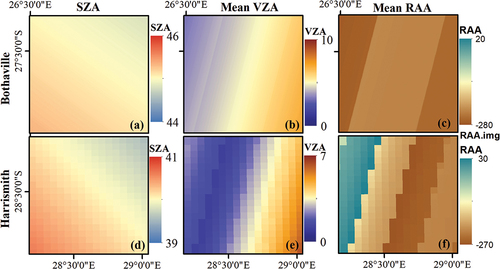
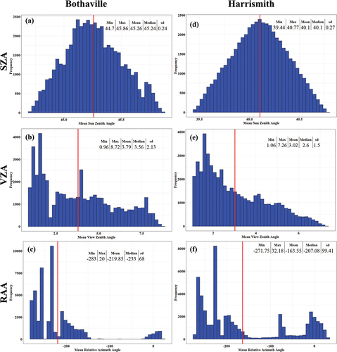
Figure 4. Summary statistics Sentinel-2 illumination and view angles in Bothaville (a–c) and Harrismith (d–f). The red line indicates the mean value for each geometric variable over 50,000 randomly sampled pixels.

In this study, multiple linear regression (Equation 1(1) $y=m_1{x}_1+m_2{x}_2+\dots +m_n{x}_n+b$(1) ) and coefficient of determination adjusted for the degree of freedom, adjusted R², were used to evaluate how much of the reflectance variation is explained by sensor view and illumination per-pixel variation using mean SZA, VZA, and RAA as predictor variables (x), and each spectral band as the response variable (y). RAA was calculated as a difference between SAA and VAA.

(1) $y=m_1{x}_1+m_2{x}_2+\dots +m_n{x}_n+b$(1)

where $y$ is the response variable (i.e. surface reflectance of each spectral band), and $x_{1\dots n}$ are predictor variables (SZA, VZA, RAA), $m_1$ represent regression coefficients, while $b$ is the intercept. The regression coefficient, i.e. the partial derivative of the response variable for each predictor variable, measures the linear sensitivity of $y$ to inputs $x_{i\dots n}$ (Mohanty and Codell 2002). Adjusted R² was used to assess the relationship between the response variable and predictor variables. In contrast, the F-statistic p-value was used to determine the significance of the relationships at α = 0.05.

3.3. Statistical analysis experiments

3.3.1. Random Forest regression algorithm

The retrieval of BVs considered here, i.e. LAI, LC_ab, and CCC, was performed using Random Forest (RF) (Breiman 2001) within the “randomForest” R-statistics package (Tierney 2012; Liaw and Wiener 2002). RF is a popular tree-based MLRA that utilizes bagging to repeatedly and independently build multiple decision trees using a subset of random training samples generated using resampling with replacement out of the original sample (Fawagreh, Gaber, and Elyan 2014; Breiman 2001). From all the training data (i.e. 70%), about 64% are kept for model building (i.e. in-bag samples), while model performance evaluation and variable importance are performed with the remaining 36% (i.e. out-of-bag or OOB samples) (Gislason, Benediktsson, and Sveinsson 2006). For each predictor, variable importance is computed by assessing the %IncMSE (Percent Increase in Mean Squared Error) when permuting OOB samples while keeping all other variables constant. The predictive power of the variables is assessed with %IncMSE, i.e. also used as a ranking measure for the various variables. For example, a variable is deemed significant if its exclusion from the model causes a considerable reduction in prediction accuracy. Essentially, a predictor with a high importance score strongly correlates with the response variable or predictive power (Mutanga, Adam, and Cho 2012). The tuning parameters, i.e. ntree (number of trees) and mtry (the number of variables for each split), were determined using the Grid-search approach using values from 100 to 500 with an interval of 10, and from 1 to p (i.e. number of predictors) with a single interval, respectively.

3.3.2. Input variables

The input variables to the Random Forest (RF) regression algorithm were divided into five (5) experimental scenarios (Table 1). The per-pixel view and illumination geometries, i.e. SZA, mean of VZA and RAA (i.e. calculated as the difference between SAA and VAA), were obtained as raster layers from the Sentinel-2 MSI product. At the same time, the MSI spectral bands were used to compute carefully selected red-edge spectral vegetation indices (SVIs, see Table 2) based on their previous empirical relationship with the BVs considered in the current study (Viña et al. 2011; Schlemmer et al., 2013; Pasqualotto et al., 2019; Delegido et al., 2011; Nguy-Robertson et al. 2012). All SVIs were calculated in the Sentinel-2 Toolbox within Sentinel Application Platform (SNAP) v8.0 software (http://step.esa.int, accessed 10 November 2020). Since the variables had varying values, they were normalized using scale and center approaches in the “mlr” R-package.

Table 1. The various experimental scenarios were designed by excluding and including view and illumination geometry from commonly used radiometric inputs (i.e. spectral bands and vegetation indices).

Scenario	Input variables	Description of input variables
SB (p = 10)	Spectral Bands	Only spectral bands (defined in Section 3.1.2) were used.
SB + Angles (p = 13)	Spectral Bands and Angles	Spectral bands combined with the cosine of view/illumination geometries (Angles), i.e. Sun Zenith Angle (SZA), mean View Azimuth Angle (VAA), and the Relative Azimuth Angle (RAA).
SVIs (p = 10)	Spectral Vegetation Indices	Only the spectral vegetation indices were used.
SVIs + Angles (p = 13)	SVIs and Angles	SVIs combined with the Angles, i.e. SZA, VAA, and mean RAA, were used.
Avar (p = 23)	All Variables	All input variables (described above) were used.

Table 2. The red-edge indices from Sentinel-2 MSI data.

Index	Equation	Reference
Normalized Difference Index	$NDI45=\frac{R_{705}-R_{665}}{R_{705}+R_{665}}$	Delegido et al. (2011)
Meris Terrestrial Chlorophyll Index	$MTCI=\frac{R_{740}-R_{705}}{R_{740}-R_{665}}$	Dash and Curran (2005)
Modified Chlorophyll Absorption Ratio Index	$MCARI=[(R_{705}-R_{665})-0.2\times \left(R_{705}-R_{560}\right)]\times \left(\frac{R_{705}}{R_{665}}\right)$	Daughtry et al., (2000)
Red-Edge Inflection Point Index	$REIP=700+40\times (\frac{(R_{665}-R_{783})/2-R_{705})}{(R_{740}+R_{705})}$	Guyot and Baret, (1988)
Sentinel-2 Red-Edge Position Index	$S2REIP=705+35\times (\frac{((R_{665}-R_{783})/2-R_{705})}{(R_{740}+R_{705})}$	Frampton et al., (2013)
Inverted Red-Edge Chlorophyll Index	$IRECI=\frac{R_{783}-R_{665}}{R_{705}+R_{740}}$	Frampton et al., (2013)
Red-edge Chlorophyll Index (CIrededge)	$C{I}_{red-edge}=\frac{R_{NIR}}{R_{RE}}-1$	Gitelson et al., (2003)
Red Edge Relative Indices (RERI) @ 705 nm	$RER{I}_{\left[705\right]}=\frac{R_{705}-R_{665}}{R_{865}}$	XU et al. (2019)
Red Edge Relative Indices (RERI) @ 783 nm	$RER{I}_{\left[783\right]}=\frac{R_{783}-R_{705}}{R_{865}}$	XU et al. (2019)
Simple Sentinel-2 LAI Index	$SeLI=\frac{R_{865}-R_{705}}{R_{865}+R_{705}}$	Pasqualotto et al., (2019)

3.3.3. Model calibration and testing

The in situ data from Harrismith data were split into 70% calibration (i.e. training) vs 30% testing (i.e. validation) using stratified-random sampling to represent all crops at the study site proportionally. Then, the 70% calibration data were combined with Bothaville data to form the calibration data for the study, while 30% was held-out for independent testing of the models. Using the pooled calibration data from the two sites, nested k-fold cross-validation (cv), where two nested k-fold cv resampling, were used for hyperparameter tuning (k = 10) and model calibration and testing (k = 5), respectively. k-fold cross-validation (cv) randomly divides the dataset into equal number of sub-datasets according to k. Then, k-1 sub-datasets constitute a training dataset, while one kth sub-dataset is the validation dataset. Using one of the k sub-datasets at each iteration, i.e. k times, the final estimation value is formed by aggregating all the validation steps. The nested k-fold cv resampling ensured that all pooled data from both study sites were used to calibrate and test the RF models (Shah et al. 2019; Verrelst et al. 2015). The cv resampling for model calibration and testing was performed with 100 iterations to reduce variability and increase the model’s predictive ability on unseen data.

3.3.4. Prediction accuracy metrics

The prediction accuracies for each Random Forest (RF) model, constructed using various experimental scenarios, were assessed with the recommended metrics by Richter et al. (2012). These metrics are R² (coefficient of determination), RMSE (root mean squared error), MAE (mean absolute error), and RRMSE (relative RMSE) (Equations 2(2) $R^2=\hspace{0.17em}\frac{\sum {(y_i^n-{\bar{y}}_i)}^2}{\sum {(y_i-{\bar{y}}_i)}^2}$(2) –6(6) $\%BIAS={\displaystyle {\sum }_{i=1}^n(x_i-y_i)}/{\displaystyle {\sum }_{i=1}^n(x_i)}$(6) ). The R² calculates the amount of the response variable (e.g. CCC) variance explained by the predictors (e.g. spectral bands). The RMSE and MAE, on the other hand, measure the degree of error between predictions and observations in the units of the BVs, i.e. m² m⁻² for LAI and µg cm⁻² for LC_ab and CCC. The RRMSE is used for comparing different variables or ranges. RRMSE values of ≤10% are indicative of Excellent predictions, and 10% < RRMSE ≤20% are Good predictions (Richter et al. 2012). Lastly, percentage Bias (%Bias) measures the model’s tendency to overestimate or underestimate a specific BV. A model is deemed accurate when the %Bias is close to 0% (Gara et al. 2019). Prediction accuracy assessment was assessed using R-statistics version 4.1.2 (Tierney 2012) packages “Metrics” (https://cran.r-project.org/web/packages/Metrics/index.html, accessed 18 July 2021) and “Fgmutils” (https://rdrr.io/cran/Fgmutils/, accessed 18 July 2021).

(2) $R^2=\hspace{0.17em}\frac{\sum {(y_i^n-{\bar{y}}_i)}^2}{\sum {(y_i-{\bar{y}}_i)}^2}$(2)

(3) $RMSE=\hspace{0.17em}\sqrt{\frac{1}{n}\hspace{0.17em}{\sum }_{i=1}^N{(x_{i\hspace{0.17em}}-\hspace{0.17em}{y}_i)}^2\hspace{0.17em}}$(3)

(4) $RRMSE=\frac{RMSE}{{\bar{x}}_i\hspace{0.17em}}$(4)

(5) $MAE=\hspace{0.17em}\frac{1}{n}{\sum }_{i=1}^n\left|x_i-\hspace{0.17em}{y}_i\right|$(5)

(6) $\%BIAS={\displaystyle {\sum }_{i=1}^n(x_i-y_i)}/{\displaystyle {\sum }_{i=1}^n(x_i)}$(6)

where x_i denotes the observed BV (e.g. CCC), and y_i denotes the predicted BV (e.g. CCC), ${\bar{x}}_i$ and ${\bar{y}}_i$ are the means of the observed (or measured) and predicted BV, respectively. N in Equation 3(3) $RMSE=\hspace{0.17em}\sqrt{\frac{1}{n}\hspace{0.17em}{\sum }_{i=1}^N{(x_{i\hspace{0.17em}}-\hspace{0.17em}{y}_i)}^2\hspace{0.17em}}$(3) is the number of errors and n is the sample size.

4. Results

4.1. Spectral variability explained by the view and illumination geometry

To determine the amount of spectral variability explained by the view and illumination geometry variables, we assessed the pixel-wise relationship of the geometries and each spectral band using multiple linear regression and coefficient of variation adjusted for the degree of freedom (adjusted R²). The results (Table 3) show that there is a significant relationship between view and illumination geometric covariates and Sentinel-2 spectral bands (p-value <2.2e-16). The adjusted R² values were between 0.30 and 0.43; therefore, view and illumination geometry covariates (i.e. SZA, VZA, RAA) explained 30% to 43% of spectral variability. B4, B2, and B7 had the lowest adjusted R² values of 0.30 ≤ 0.34, while B3, B5, B6, B8, B8AB8A, and B12 had adjusted R² values of 0.35 < 0.4, and B11 had adjusted R² value of >0.4. The same is observed in Harrismith for VIS bands B2, B3, and B4 and NIR band B8, but the geometric variables explained <30% of surface reflectance variability in B5, B6, B7B7, and B8A, while they explained >40% of surface reflectance variability in B11 and B12. In Harrismith, the significant geometric variables at α < 0.05were RAA in B2, RAA and VZA in B3, and SZA and VZA in B7, while all the other bands were influenced significantly by all geometric variables, i.e. SZA VZA, and RAA. Similarly, in Bothaville, all the geometric variables were significant at α < 0.05.

Table 3. The amount of spectral variability explained by the geometric variables based on multiple linear regression.

		B2	B3	B4	B5	B6	B7	B8	B8A	B11	B12
Bothaville	Adj. R^2	0.32	0.36	0.30	0.35	0.35	0.34	0.35	0.36	0.43	0.37
	p-Value	<2.2e-16	<2.2e-16	<2.2e-16	<2.2e-16	<2.2e-16	<2.2e-16	<2.2e-16	<2.2e-16	<2.2e-16	<2.2e-16
Harrismith	Adj. R^2	0.35	0.32	0.37	0.25	0.19	0.21	0.28	0.36	0.47	0.42
	p-Value	<2.2e-16	2.709e-15	<2.2e-16	9.297e-12	1.076e-08	1.624e-09	2.718e-13	<2.2e-16	<2.2e-16	<2.2e-16

Adj. R² denotes Adjusted R².

4.2. Predictive performance of Sentinel-2 covariates

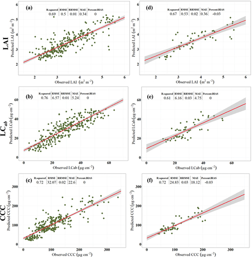
Five experimental scenarios, designed based on the different combinations of Sentinel-2 MSI co-variates, were assessed for their performance in retrieving LAI, LCab, and CCC using Random Forest (RF) regression algorithm. The results were confirmed by applying the calibrated models on two test datasets, i.e. one selected through five5-fold cross-validation (cv) using the pooled data from two study sites (hereafter, cross-validation test dataset) and an independent held-out (i.e. unseen) dataset from Harrismith (hereafter, independent held-out test dataset). Generally, the results (Table 4) indicate that, among the compared experimental scenarios, the SB + Angles and SVIs + Angles scenarios provided the most robust retrievals of all the BVs considered here, except for CCC, where SB + Angles and Avar provided better results than other scenarios. The LAI retrieval models using SB + Angles and SVIs + Angles yielded excellent predictive performance with RMSE of 0.50 and 0.43 m² m⁻². Moreover, they explained the most significant variability of LAI within the two test datasets, i.e. 69% and 67% for cross-validation test data and independent held-out (i.e. unseen) data, respectively. These performances were closer to Avar, which achieved RMSEs of 0.52 and 0.55 m² m⁻² and R² of 0.66 and 0.67, respectively. In contract, the predictive performance of input scenarios where the per-pixel view and illumination geometry covariates were excluded, i.e. SB and SVIs, were relatively inferior, achieving RMSE >0.60 m² m⁻² and R² <0.60) for both test datasets.

Table 4. The performance of various Sentinel-2 input variables in retrieving various crop parameters using Random Forest (RF) with two test datasets, i.e. cross-validation data pooled from the two sites and independent test data from Harrismith (in brackets).

		SB	SVIs	SB + Angles	SVIs + Angles	Avar
LAI	R^2	0.59 (0.49)	0.52 (0.58)	0.69 (0.66)	0.67 (0.67)	0.66 (0.67)
	RMSE	0.57 (0.65)	0.62 (0.62)	0.50 (0.55)	0.51 (0.53)	0.52 (0.55)
	RRMSE	0.01 (0.02)	0.01 (0.02)	0.01 (0.02)	0.01 (0.02)	0.01 (0.02)
	MAE	0.41 (0.48)	0.44 (0.44)	0.34 (0.37)	0.36 (0.36)	0.36 (0.37)
	%Bias	0.00 (−0.03)	0.00 (−0.04)	0.00 (−0.03)	0.00 (−0.03)	0.00 (−0.04)
LCab	R^2	0.71 (0.49)	0.74 (0.59)	0.72 (0.49)	0.76 (0.61)	0.74 (0.58)
	RMSE	7.16 (7.18)	6.75 (6.31)	7.01 (7.06)	6.57 (6.16)	6.69 (6.43)
	RRMSE	0.01 (0.03)	0.01 (0.03)	0.01 (0.03)	0.01 (0.03)	0.01 (0.03)
	MAE	5.68 (5.57)	5.30 (4.88)	5.56 (5.32)	5.24 (4.75)	5.57 (4.95)
	%Bias	− 0.01 (0.00)	−0.01 (−0.01)	0.00 (0.00)	0.00 (0.00)	0.00 (0.00)
CCC	R^2	0.69 (0.69)	0.67 (0.67)	0.72 (0.69)	0.72 (0.72)	0.72 (0.72)
	RMSE	33.48 (26.48)	34.52 (27.86)	32.07 (26.63)	32.37 (25.98)	32.36 (24.83)
	RRMSE	0.02 (0.04)	0.02 (0.04)	0.02 (0.04)	0.02 (0.04)	0.02 (0.03)
	MAE	23.31 (20.96)	23.88 (19.38)	22.60 (20.16)	22.39 (18.19)	22.68 (18.12)
	%Bias	0.00 (0.00)	−0.01 (−0.06)	0.00 (−0.02)	−0.01 (−0.04)	−0.01 (−0.03)

The bold values indicate the best (i.e. lowest) RMSE achieved by the input variable scenario for each biophysical/biochemical variable (BV).

Interestingly, the best predictive performance for LC_ab was achieved with SVIs + Angles with RMSE of 6.57 µg cm ⁻² (R²: 0.76) and 6.16 µg cm ⁻² (R²: 0.61), respectively. The next better predictive performance was achieved by SVIs and Avar, while SB + Angles and SB were slightly worse. Similar to LAI models, the CCC retrieval models built with input scenarios that incorporated per-pixel view and illumination geometry covariates, i.e. SB + Angles, SVIs + Angles, and Avar, were better than those that used scenarios which did not contain any geometric variables, i.e. SB and SVIs.

Overall, the predictive performance of the BV models was consistent between the two test datasets, demonstrating the contribution of per-pixel view and illumination geometry covariates in improving the robustness of BV retrievals. However, contrary to LAI results, the SVIs-LC_ab model outperformed the scenarios incorporating per-pixel view and illumination geometry covariates, i.e. SB + Angles and Avar. As demonstrated by SB + Angles, SVIs + Angles, and Avar results, incorporating pixel-wise geometric information led to robust LAI, LC_ab, and CCC predictions using Random Forest (RF). It can also be deduced that carefully chosen red-edge vegetation indices have high information content considering SVIs’ next better performance after SVIs + Angles in the retrieval of LC_ab. In contrast, spectral reflectance bands were relatively superior in retrieving LAI and CCC. All input variable scenarios achieved RRMSE of <5%, thus within the GCOS limit of 10% (GCOS, 2009).

As shown in Figure 5, all the experimental scenarios resulted in underestimations, to some extent, of all the BVs considered. The LAI seems to saturate at ~5 m² m⁻² with a %Bias of up to 4% with the independent test data. The retrievals of LC_ab saturate at ~50 µg cm⁻². Finally, using the cross-validation test dataset, the CCC saturates at ~250 µg cm⁻², while the same occurs at relatively lower values, i.e. ~200 µg cm⁻² with the independent held-out test dataset. It should be noted, however, that the range was lower in the latter test dataset. As shown in Table 4, the %Bias was slightly worse in models which did not incorporate per-pixel view and illumination geometry covariates, i.e. up to 6%, across all BVs. Overall, the results from the two test datasets indicate that incorporating pixel-wise sensor view and illumination geometries reduced the %Bias for LAI, LC_ab and CCC.

Figure 5. Scatterplots for the best Random Forest (RF) models for retrieving various BVs using various Sentinel-2 covariates, cross-validation test dataset pooled from Bothaville and Harrismith (i.e. a–c) and an independent held-out (i.e. 30%) dataset from Harrismith (i.e. d–f). SB + Angles achieved the best LAI and CCC predictive accuracy with cross-validation test datasets (i.e. a and c), while SVIs + Angles resulted in superior predictive accuracy for LC_ab with both test datasets (i.e. b and e), and for LAI with the Independent held-out (i.e. 30%) dataset (i.e. d). Avar achieved superior predictive accuracy for CCC with the independent held-out dataset (i.e. f).

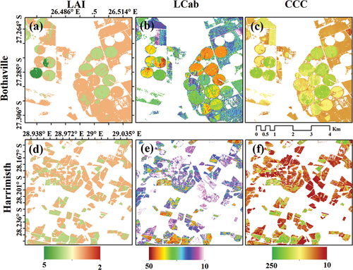
The spatial distribution maps of crop biophysical and biochemical variables are presented in Figure 6. The maps were derived with the best RF models, which incorporated geometric variables, i.e. SB + Angles and SVIs + Angles (see Table 4)

Figure 6. Spatial distribution of crop biophysical and biochemical variables for Bothaville (a–c) and Harrismith (d–f). The LAI and CCC maps in (a) and (c) were achieved with SB + Angles, while LC_ab in (b) and (e) SVIs + Angles. Avar was used to map CCC in (f).

4.3. Variable importance

We evaluated the contribution of each input variable to the BV retrieval models with the Random Forest (RF) variable importance measure, i.e. the Percentage Increase in Mean Squared Error (%IncMSE). For brevity, we exclude the results for SB and SVIs which did not incorporate sensor view and illumination geometries as covariates because our interest was on the contribution of geometric covariates. Nevertheless, the results for SB were reported in our previous work (Kganyago, Mhangara, and Adjorlolo 2021). Generally, all evaluated input variable scenarios (i.e. that incorporated geometric covariates in the modeling of BVs) show the considerable importance (or influence) of the per-pixel illumination and viewing geometries on crop BV retrieval (Figure 7). The RF variable importance results for LAI (Figure 7a,d,g) show that VZA and SZA were the topmost important input variables, consistently showing a high %IncMSE of >20% when using the SB + Angles and SVIs + Angles, while they had an average %IncMSE of ≥10%<20% when using Avar. The other geometric covariate, i.e. RAA, had an average %IncMSE (i.e. ≥10% <20%) in all the scenarios, along B3, B8A, and B5, and SWIR bands B11 and B12 when using SB + Angles, CI_{RE_740}, MTCI, NDI45, MCARI, IRECI, and RERI₇₀₅ when using SVIs + Angles, and CI_green, CI_{RE_740}, B3, MTCI, B8A, and B12 when using Avar. The visible bands, B2 and B4, were among the highly influential variables in the LAI model using SB + Angles (i.e. %IncMSE >20%), while B2 was among the top three influential variables in the LAI model using Avar.

Figure 7. Top 10 important variables (high to low) for retrieving LAI, LC_ab, and CCC using each experimental scenario identified with Random Forest (RF) and fivefold cross-validation with 100 iterations.

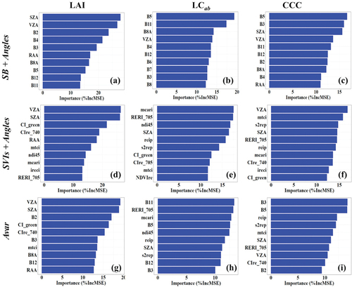
In Figure 7b,e,h, the contribution of geometric covariates is also evident, where when using SB + Angles as input variables, VZA was the only geometric variable featured in the top 10 most important variables. When using SVI + Angles and Avar, only SZA (among other geometric covariates) was the topmost influential variable. The radiometric variables, B5, B11, B8A, and B4, were relatively more influential in the SB + Angles-LC_ab models, while MCARI, RERI₇₀₅, NDI45, REIP, and S2REP were among the highly influential among the SVI + Angles variables. For Avar, B11, RERI₇₀₅, MCARI, B5, NDI45, and REIP had the most influence on the LC_ab model. Similar to LAI, the RF variable importance results (Figures 7c,f,i) show that VZA and SZA seem to play a pivotal role in the CCC retrieval, where they were consistently featured among the most important variables in all experimental scenarios, SB + Angles, SVI + Angles and Avar. In addition to these geometric covariates, B5, B3, B11, and B12 were the topmost variables when using SB + Angles. On the other hand, MTCI, S2REP, RERI₇₀₅, and REIP have ranked topmost in SVI + Angles, while B5, B3, S2REP, REIP, and MTCI were topmost in Avar.

5. Discussions

Understanding the contribution of view and illumination geometry to the accuracy of retrieving crop BVs is critical for reducing the retrieval uncertainty of these BVs by accounting for geometric sources of variability in the reflectance data. As Jacquemoud et al. (2009) note, the view and illumination geometry profoundly impact the canopy reflectance. Therefore, incorporating geometric variables provides an opportunity to exploit additional structural information content or to minimize their effects where it causes noise (Roy et al. 2017b; Verrelst et al. 2008). Previous studies focused on the effects of varying illumination conditions due to topography (Martín-Ortega, García-Montero, and Sibelet 2020; Matsushita et al. 2007), correction of surface anisotropy effects for inter-sensor comparisons (Roy et al. 2017b; Roy, Li, and Zhang 2017a) and global effect of either view or illumination geometry on vegetation reflectance (Pocewicz et al. 2007; Verrelst et al. 2008; Ranson, Daughtry, and Biehl 1986), without considering the within-scene, per-pixel view, and illumination geometry contribution to the retrieval of BVs.

To address this gap, we evaluated various input variable scenarios (see Table 2) for crop BVs retrieval using the Random Forest (RF) regression algorithm. These experimental scenarios were designed to elucidate the contribution of view and illumination geometries to the crop BVs retrieval accuracy. Since Sentinel-2 has a relatively wide field of view (FOV), i.e. ~20.6° (i.e. ~290 km), compared to relatively narrow FOV sensors such as Landsat-8 OLI, i.e. ~15° (~190 km), it is prone to within scene view and illumination geometry variations (see Figure 2), with potential to affect BVs retrieval. To highlight view and illumination geometry contribution to model performance practically, we assessed the predictive power of all input variables per experimental scenario using RF variable importance (%IncMSE). Furthermore, the adjusted R² of multiple linear regression was used to determine the amount of spectral reflectance variation explained by geometric covariates (see Table 4).

5.1. Contribution of geometric covariates to BVs retrieval accuracy

Generally, the results showed that the experimental scenarios incorporating per-pixel geometric covariates, i.e. SZA, VZA, and RAA, yielded robust retrievals of LAI, LC_ab, and CCC. For example, adding geometric covariates to the standard input variables for retrieval of LAI using cross-validation test data, i.e. spectral bands (SB) and spectral vegetation indices (SVIs), showed improvements in R² of 10% and 15%, respectively. At the same time, RMSEs improved by 0.07 m² m⁻² and 0.11 m² m⁻², respectively. These improvements also manifest in the derived spatial distribution maps, which show with-field and between-field spatial variations in LAI when geometric variables are excluded (i.e. SB and SVIs) and included (i.e. SB + Angles and SVIs + Angles) in the model (see Figure S1 and S2). The independent held-out test dataset showed improvements in R² by 17% and 9% and RMSEs by 0.1 and 0.09 m² m⁻². On the other hand, relatively lower improvements were realized for CCC, where SB + Angles achieved improvements of 3% in explained variability and RMSE improvements by only 1.41 µg cm ⁻² using a cross-validation test dataset. In contrast, the independent held-out dataset showed no improvements (instead, a decline in RMSE by 0.15 µg cm ⁻² was observed). Using SVIs + Angles, 5% improvements in explained variability were achieved using both test datasets, respectively, while RMSEs improved by 2.15 and 1.88 µg cm ⁻² for the cross-validation and independent held-out test datasets, respectively. For LC_ab, the improvements in R² and RMSE were marginal and possibly trivial. When the geometric covariates were added to SB (i.e. SB + Angles), only a 1% increase in R² and RMSE increase by 0.15 and 0.12 µg cm ⁻² were achieved with both test datasets, respectively. Similarly, SVIs + Angles led to a 2% improvement in explained variability and RMSE improvements by 0.18 and 0.15 µg cm ⁻² for the cross-validation and independent held-out test datasets, respectively. Generally, LC_ab (measured at the leaf level) is difficult to estimate from canopy reflectance, which contains the influence of the background, plant structural and biochemical traits. That is why the variability introduced by geometric covariates was not crucial for LC_ab estimation in this study. Consequently, spatial distribution maps derived with standard variables, i.e. SB and SVIs show no apparent differences (see Figures S1 and S2).

Indeed, the SVIs offer a simple and rapid assessment of crop health, with several studies showing their relationship with and accuracy in retrieving crop BVs (Jay et al. 2017; Main et al. 2011; Kooistra and Clevers 2016; Haboudane et al. 2008, 2004). In retrieving the LAI, CCC, and canopy nitrogen content of sugar beet crops, Jay et al. (2017) found that the SVIs perform equivalent or slightly better than PROSAIL inversion. It is, therefore, not surprising that the SVIs such as MTCI, S2REIP, REIP, NDI45, MCARI, and CI_{RE_740} were consistently ranked among the top variables when using Avar across all BVs. Also, the SVIs scenario was superior to SB, SB + Angles, and Avar in retrieving LC_ab. Vegetation indices such as MTCI, RVI and NDI45 were previously found to be highly correlated to LAI and chlorophyll content (Viña et al. 2011). In agreement, Shah et al. (2019) found that MTCI is one of the best-performing SVIs with an R² of 0.86 and an RMSE of 6.07 µg cm⁻² in estimating Wheat LC_ab due to its sensitivity to wide-ranging chlorophyll content. Similarly, CLEVERS and Gitelson (2013) observed that the MTCI is an accurate estimator of Canopy Chlorophyll Content (CCC) and nitrogen (N) content due to its linear relationship with these BVs. The results in this study are consistent with these previous studies and others (Main et al. 2011), using cross-validation and independent held-out test datasets. Moreover, SVIs selected in this study yielded comparative results to SB, except in exceptional cases, i.e. the SVIs-LC_ab model, where the former was superior. Their excellent performance can be attributed to their relatively low sensitivity to background soils, and residual atmospheric effects, which affect most VIS/NIR indices (Liu, Pattey, and Jégo 2012). However, their relatively low performance relative to SVIs + Angles signifies their sensitivity to per-pixel view and illumination geometry, as consistently reported previously (Verrelst et al. 2008; Jay et al. 2017). For example, Verrelst et al. (2008) found that broadband and narrowband greenness indices exhibit significant sensitivity to view geometry. In the current study, when per-pixel view and illumination geometric covariates were incorporated (i.e. SVIs + Angles), the variability explained improved from 52% (58%), 74% (59%) and 67% (67%) when using SVIs only to 67% (67%), 76% (61%), and 72% (72%) for LAI, LC_ab, and CCC, respectively, using cross-validation test (independent held-out test) datasets. Moreover, when per-pixel view and illumination geometric covariates were incorporated into SB (i.e. SB + Angles), the variability explained improved from 59% (49%), 71% (49%), and 69% (69%) to 69% (66%), 72% (49%), 72% (69%) for LAI, LC_ab, and CCC, respectively, using cross-validation test (independent held-out test) datasets. These results signify that the per-pixel view and illumination geometry affect the upwelling radiance from crop canopies as determined by the interaction of various leaf and canopy traits. Such effects were not accounted for during atmospheric correction and thus were propagated to surface reflectance.

Therefore, incorporating pixel-wise view and illumination geometry into the retrieval of BVs is reasonable since it is one of the factors influencing the canopy reflectance. In this study, its inclusion to SB and SVIs ensured that the variability in reflectance caused by the view and illumination geometry is accounted for, thus leading to improved predictive accuracy relative to using the SB or SVIs only. As shown by the multiple linear regression analysis (Table 3), more than 30% of the variability in all Sentinel-2 spectral bands was explained by the per-pixel variation in view and illumination geometries at a 5% significant level (p < 2.2e-16). A previous study (Verrelst et al. 2008) found that topographic and illumination geometry accounted for about 13% of SVIs’ variability. Similarly, Rahman et al. (1999) found that the canopy reflectance of rice and wheat varies significantly with view geometry, where the change in view geometry resulted in different spectral responses due to the exposed soils and vegetation for each geometry. Nagol et al. (2015) found that the effect of narrow VZA (i.e. ±7°) in Landsat data resulted in non-negligible variations in reflectance, i.e. 20%.

5.2. The predictive power of the geometric covariates

The additional predictive power provided by the geometric covariates was also shown by the Random Forest (RF) variable importance results, where one or more view and illumination geometry covariates were among highly informative variables in all biophysical and biochemical models (see Figure 7). Among the geometric covariates, VZA and SZA were the most influential in retrieving LAI and CCC. In particular, all scenarios showed the high influence (ranked by their %IncMSE) of SZA and VZA for the retrieval of LAI and CCC. Other scenarios, i.e. LC_ab retrieval with SB + Angles, showed that VZA was the only geometric variable featured in the top 10 important variables (see Figure 7). In contrast, the retrieval of LC_ab using SVIs + Angles and Avar showed SZA as the only geometric variable with a strong influence on the model. The findings in this study correspond to Verrelst et al. (2008) that the spectral response of plant canopies is significantly affected by the sensor view geometry, affecting the accuracy of retrieved BVs.

Moreover, the findings not only ascertain previous studies that demonstrated solar illumination effects on SVIs (Galvao et al. 2011) but also indicate that per-pixel SZA can contribute essential additional information that improves the predictive power of SVIs, thus reducing the uncertainty in BV retrieval. SZA contains per-pixel geometric information of the incident radiation. Critically, within-scene SZA changes with the crop growth stages (i.e. time of year); hence, ignoring its effects may lead to inconsistent BV retrieval and subsequent incorrect interpretations. For example, Galvao et al. (2011) found that intra-annual variability in enhanced vegetation index (EVI) from MODIS and nadir Hyperion was regulated by illumination effects than actual changes in LAI. In the context of precision agriculture and crop monitoring, such false alarms, i.e. caused by geometric variability, have profound implications. It may lead to incorrect crop condition diagnosis that can lead to wasteful use of scarce and expensive farm inputs (e.g. irrigation water, pesticides, and fertilizers) and poor yields as the stressed crops are not timely and adequately remedied. This can potentially lead to loss of trust in remotely sensed crop BVs for agronomic applications.

As one of the factors affecting reflectance variability (see Table 3), per-pixel geometric information has been ignored in retrieving BVs with optical satellite images. This may be a consequence of the absence of spatially explicit view and illumination information by heritage missions such as Landsat and AVHRR that largely drove BV retrieval techniques’ development. As the results in this study have shown, the per-pixel geometric variables explain a reasonable amount of variability in satellite-based canopy reflectance; hence it should be incorporated into MLRA models to improve the accuracy and reliability of crop BVs. Therefore, it is reasonable to deduce that spectral bands or vegetation indices combined with geometric covariates offer the most significant prospects of reliable prescription maps for precision agriculture technologies, such as variable rate application (VRA) of fertilizer and pesticides, and to aid agronomic decisions. Although SNAP biophysical processor, based on PROSAIL LUT and ANN incorporate these geometric variables (Weiss and Baret 2020), validation studies (Kganyago et al. 2020; Xie et al. 2019; Djamai et al. 2019) have shown that the product is associated with significant uncertainties which render its site-specific agronomic application questionable. Therefore, based on the results here and in line with Combal et al. (2003), it can be assumed that locally parameterizing the PROSAIL LUT (using prior information) may reduce high uncertainty in BV retrieval and show the contribution of the geometric covariates.

Therefore, models with SB or red-edge SVIs and pixel-wise geometric covariates are more promising for LAI and CCC retrieval (see Figures S1 and S2). This is attractive for precision agriculture applications since these geometric covariates come standard with Sentinel-2 products and can be conveniently incorporated into BV retrieval models to account for per-pixel view and illumination geometry effects and achieve unprecedented accuracies and temporal consistency for relatively wide FOV sensors such as Sentinel-2.

5.3. Limitations of the study

Despite the promising results, the main limitation of this study was that the applicability of MLRA models constructed with experimental data is limited by the representativeness of such data (Weiss, Jacob, and Duveiller 2020); thus, the results obtained here may be crop-type, region- and phenology-specific. Therefore, further experiments in different geographic locations and periods are required to ascertain the contribution of per-pixel geometric covariates. Moreover, simulated data using RTMs is recommended for future works to make the models widely applicable and assess the geometric variables’ influence on BVs. Nonetheless, the multiple linear regression analysis showed a non-negligible influence on surface reflectance of the considered crop types, while RF variable importance indicated that they are influential to the model performance and accuracy of retrieving LAI, LC_ab and CCC. Overall, this study found that per-pixel view and illumination geometric covariates improve MLRA crop BVs retrieval. Future studies should explore the optimization of Sentinel-2 feature space (including derived vegetation indices using feature selection to avoid potential collinearity of predictors and improve the practical prospects of combining geometric and radiometric variables in retrieving crop BVs.

6. Conclusion

This study evaluated the influence of Sentinel-2 pixel-wise sensor view and solar illumination geometry on the accuracy of estimating crop biophysical and biochemical variables relevant for precision agriculture and crop monitoring, i.e. LAI, LC_ab, and CCC. Generally, the results showed that the experimental scenarios incorporating per-pixel geometric covariates, i.e. SZA, VZA, and RAA, yielded robust retrievals of LAI and CCC, while there was a negligible improvement (i.e. R²: 1–2%) in LC_ab retrieval accuracy. In particular, standard input variables, such as spectral bands and spectral vegetation indices, to biophysical retrieval models, combined with geometric covariates resulted in the best (i.e. lowest) RMSE for all considered crop BVs owing to high information content in the spectral bands and red-edge indices, and residual variability explained by the pixel-wise view and illumination geometry. The results showed that this variability exceeded 30% in all Sentinel-2 bands and sites. Moreover, variable importance assessment showed that VZA and SZA were among the topmost influential variables in retrieving all BVs. The spatially explicit view and illumination information provided with Sentinel-2 can be used as additional information to account for variability resulting from sensor and sun geometries in BV retrieval with MLRAs. This study showed that ignoring the influence of sensor and sun geometry may lead to inconsistencies in BV retrieval as the SZA changes along the cropping season, and VZA varies across the scene. Moreover, their influence on reflectance is considerable, i.e. >30%; thus, estimated BVs can be incorrectly interpreted, as shown by Galvao et al. (2011). In precision agriculture, it may lead to an inaccurate crop health diagnosis, risking wasteful use of irrigation water, pesticides and fertilizers, poor yields, and loss of trust in remotely sensed BVs for agronomic applications. Based on this study’s results, we recommend incorporating per-pixel view and illumination geometry in estimating canopy-level BVs such as LAI and CCC, especially when using wide-view sensors such as Sentinel-2. However, further tests are required to reaffirm the contribution of view and illumination geometry toward improving the crop BVs that support precision agriculture and aid agronomic decisions.

Disclosure statement

No potential conflict of interest was reported by the author(s).

Data availability statement

The data that support the findings of this study are available from the corresponding author, MK, upon reasonable request.

Supplemental data

Supplemental data for this article can be accessed online at https://doi.org/10.1080/15481603.2022.2163046.

Additional information

Funding

The work was supported by the Horizon 2020 Framework Programme [774652]; ESA Network of Resources (NoR) [66518]; University of the Witwatersrand, Johannesburg [Merit Award].

References

- Alexandridis, T. K., G. Ovakoglou, and J. G. P. W. Clevers. 2020. “Relationship Between MODIS EVI and LAI Across Time and Space.” Geocarto international 35 (13): 1385–20. doi:10.1080/10106049.2019.1573928.
- Apolo-Apolo, O. E., M. Pérez-Ruiz, J. Martínez-Guanter, and G. Egea. 2020. “A Mixed Data-Based Deep Neural Network to Estimate Leaf Area Index in Wheat Breeding Trials.” Agronomy 10 (2). doi:10.3390/agronomy10020175.
- Azodi, C. B., J. Tang, and S. H. Shiu. 2020. “Opening the Black Box: Interpretable Machine Learning for Geneticists.” Trends in Genetics 36 (6): 442–455. doi:10.1016/j.tig.2020.03.005.
- Biriukova, K., M. Celesti, A. Evdokimov, J. Pacheco-Labrador, T. Julitta, M. Migliavacca, C. Giardino, et al. 2020. “Effects of Varying Solar-View Geometry and Canopy Structure on Solar-Induced Chlorophyll Fluorescence and PRI.” International Journal of Applied Earth Observation and Geoinformation 89: 102069. doi:10.1016/j.jag.2020.102069.
- Breiman, L. 2001. “Random Forests.” Machine Learning 45 (1): 5–32. doi:10.1023/A:1010933404324.
- Clevers, J. G., and A. A. Gitelson. 2013. “Remote Estimation of Crop and Grass Chlorophyll and Nitrogen Content Using Red-Edge Bands on Sentinel-2 And-3.” International Journal of Applied Earth Observation and Geoinformation 23: 344–351. doi:10.1016/j.jag.2012.10.008.
- Clevers, J., L. Kooistra, and M. Van den Brande. 2017. “Using Sentinel-2 Data for Retrieving LAI and Leaf and Canopy Chlorophyll Content of a Potato Crop.” Remote Sensing 9 (5): 405. doi:10.3390/rs9050405.
- Combal, B., F. Baret, M. Weiss, A. Trubuil, D. Mace, A. Pragnere, R. Myneni, Y. Knyazikhin, and L. Wang. 2003. “Retrieval of Canopy Biophysical Variables from Bidirectional Reflectance: Using Prior Information to Solve the Ill-Posed Inverse Problem.” Remote Sensing of Environment 84 (1): 1–15. doi:10.1016/S0034-4257(02)00035-4.
- Cropestimatesconsortium. 2017. ”Field Crop Boundary Data Layer (Free State Province).” In Field Crop Boundary Data Layer (Free State Province), 2017, ed. CROPESTIMATESCONSORTIUM. Pretoria: Department of Agriculture, Forestry and Fisheries.
- Dash, J., and P. J. Curran. 2005. “The MERIS Terrestrial Chlorophyll Index.” International Journal of Remote Sensing 25: 5403–5413.
- Daughtry, C. S. T., C. L. Walthall, M. S. Kim, E. Brown, and J. E. McMurtrey. 2000. “Estimating Corn Leaf Chlorophyll Concentration from Leaf and Canopy Reflectance.” Remote Sensing of Environment 74: 229–239.
- Delegido, J., J. Verrelst, L. Alonso, and J. Moreno. 2011. “Evaluation of Sentinel-2 Red-Edge Bands for Empirical Estimation of Green LAI and Chlorophyll Content.” Sensors 11 (7): 7063–7081. doi:10.3390/s110707063.
- Delegido, J., J. Verrelst, C. M. Meza, J. P. Rivera, L. Alonso, and J. Moreno. 2013. “A Red-Edge Spectral Index for Remote Sensing Estimation of Green LAI Over Agroecosystems.” European Journal of Agronomy 46: 42–52. doi:10.1016/j.eja.2012.12.001.
- Dimitrov, P., I. Kamenova, E. Roumenina, L. Filchev, I. Ilieva, G. Jelev, A. Gikov, M. Banov, et al. 2019. “Estimation of Biophysical and Biochemical Variables of Winter Wheat Through Sentinel-2 Vegetation Indices.” Bulgarian Journal of Agricultural Science 25 (5): 819–832.
- Djamai, N., R. Fernandes, M. Weiss, H. Mcnairn, and K. Goïta. 2019. “Validation of the Sentinel Simplified Level 2 Product Prototype Processor (SL2P) for Mapping Cropland Biophysical Variables Using Sentinel-2/MSI and Landsat-8/OLI Data.” Remote Sensing of Environment 225: 416–430. doi:10.1016/j.rse.2019.03.020.
- Durbha, S. S., R. L. King, and N. H. Younan. 2007. “Support Vector Machines Regression for Retrieval of Leaf Area Index from Multiangle Imaging Spectroradiometer.” Remote Sensing of Environment 107 (1–2): 348–361. doi:10.1016/j.rse.2006.09.031.
- Duveiller, G., R. Lopez-Lozano, and A. Cescatti. 2015. “Exploiting the Multi-Angularity of the MODIS Temporal Signal to Identify Spatially Homogeneous Vegetation Cover: A Demonstration for Agricultural Monitoring Applications.” Remote sensing of environment 166: 61–77. doi:10.1016/j.rse.2015.06.001.
- Fawagreh, K., M. M. Gaber, and E. Elyan. 2014. “Random Forests: From Early Developments to Recent Advancements.” Systems Science & Control Engineering: An Open Access Journal 2 (1): 602–609. doi:10.1080/21642583.2014.956265.
- Fitzgerald, G., D. Rodriguez, and G. O’Leary. 2010. “Measuring and Predicting Canopy Nitrogen Nutrition in Wheat Using a Spectral Index-The Canopy Chlorophyll Content Index (CCCI).” Field Crops Research 116 (3). doi:10.1016/j.fcr.2010.01.010.
- Frampton, W. J., J. Dash, G. Watmough, and E. J. Milton. 2013. “Evaluating the Capabilities of Sentinel-2 for Quantitative Estimation of Biophysical Variables in Vegetation.” ISPRS Journal of Photogrammetry and Remote Sensing 82: 83–92. doi:10.1016/j.isprsjprs.2013.04.007.
- Galvao, L. S., J. R. dos Santos, D. A. Roberts, F. M. Breunig, M. Toomey, and Y. M. de Moura. 2011. “On Intra-Annual EVI Variability in the Dry Season of Tropical Forest: A Case Study with MODIS and Hyperspectral Data.” Remote Sensing of Environment 115 (9): 2350–2359. doi:10.1016/j.rse.2011.04.035.
- Gara, T. W., R. Darvishzadeh, A. K. Skidmore, T. Wang, and M. Heurich. 2019. “Accurate Modelling of Canopy Traits from Seasonal Sentinel-2 Imagery Based on the Vertical Distribution of Leaf Traits.” Isprs Journal of Photogrammetry and Remote Sensing 157: 108–123. doi:10.1016/j.isprsjprs.2019.09.005.
- Gascon, F., C. Bouzinac, O. Thépaut, M. Jung, B. Francesconi, J. Louis, V. Lonjou, et al. 2017. “Copernicus Sentinel-2A Calibration and Products Validation Status.” Remote Sensing 9 (6): 584. doi:10.3390/rs9060584.
- Gislason, P. O., J. A. Benediktsson, and J. R. Sveinsson. 2006. “Random Forests for Land Cover Classification.” Pattern recognition letters 27 (4): 294–300. doi:10.1016/j.patrec.2005.08.011.
- Gitelson, A. A., Y. Gritz, and M. N. Merzlyak. 2003. “Relationships Between Leaf Chlorophyll Content and Spectral Reflectance and Algorithms for Non-Destructive Chlorophyll Assessment in Higher Plant Leaves.” Journal of Plant Physiology 160 (3): 271–282. doi:10.1078/0176-1617-00887.
- Guyot, G., and F. Baret. 1988. Utilisation de la haute re´solution spectrale pour suivre l’e´tat des couverts ve´ge´taux [Utilisation of high spectral resolution for monitoring vegetation condition]. In T.-D.-G. enne and J. J. Hunt (eds.), Proceedings of 4th international colloquim spectral signatures of objects in remote sensing, proceedings of the conference held 18–22 January 1988 in Aussois (Modane), France (pp. 279–286). ESA SP-287. European Space Agency.
- Haboudane, D., J. R. Miller, E. Pattey, P. J. Zarco-Tejada, and I. B. Strachan. 2004. “Hyperspectral Vegetation Indices and Novel Algorithms for Predicting Green LAI of Crop Canopies: Modeling and Validation in the Context of Precision Agriculture.” Remote Sensing of Environment 90 (3): 337–352. doi:10.1016/j.rse.2003.12.013.
- Haboudane, D., N. Tremblay, J. R. Miller, and P. Vigneault. 2008. “Remote Estimation of Crop Chlorophyll Content Using Spectral Indices Derived from Hyperspectral Data.” IEEE Transactions on Geoscience and Remote Sensing 46 (2): 423–437. doi:10.1109/TGRS.2007.904836.
- Jacquemoud, S., W. Verhoef, F. Baret, C. Bacour, P. J. Zarco-Tejada, G. P. Asner, C. François, and S. L. Ustin. 2009. “PROSPECT+ SAIL Models: A Review of Use for Vegetation Characterisation.” Remote Sensing of Environment 113: S56–66. doi:10.1016/j.rse.2008.01.026.
- Jay, S., F. Maupas, R. Bendoula, and N. Gorretta. 2017. “Retrieving LAI, Chlorophyll and Nitrogen Contents in Sugar Beet Crops from Multi-Angular Optical Remote Sensing: Comparison of Vegetation Indices and PROSAIL Inversion for Field Phenotyping.” Field Crops Research 210: 33–46. doi:10.1016/j.fcr.2017.05.005.
- Karimi, S., A. A. Sadraddini, A. H. Nazemi, T. Xu, and A. F. Fard. 2018. “Generalizability of Gene Expression Programming and Random Forest Methodologies in Estimating Cropland and Grassland Leaf Area Index.” Computers and Electronics in Agriculture 144: 232–240. doi:10.1016/j.compag.2017.12.007.
- Kganyago, M., C. Adjorlolo, and P.Mhangara. 2022. “Exploring Transferable Techniques to Retrieve Crop Biophysical and Biochemical Variables Using Sentinel-2 Data.” Remote Sensing 14 (16): 3968. doi:10.3390/rs14163968.
- Kganyago, M., P. Mhangara, and C. Adjorlolo. 2021. “Estimating Crop Biophysical Parameters Using Machine Learning Algorithms and Sentinel-2 Imagery.” Remote Sensing 13 (21): 1–21. doi:10.3390/rs13214314.
- Kganyago, M., P. Mhangara, T. Alexandridis, G. Laneve, G. Ovakoglou, and N. Mashiyi. 2020. “Validation of Sentinel-2 Leaf Area Index (LAI) Product Derived from SNAP Toolbox and Its Comparison with Global LAI Products in an African Semi-Arid Agricultural Landscape.” Remote Sensing Letters 11 (10): 883–892. doi:10.1080/2150704X.2020.1767823.
- Kneubühler, M., B. Koetz, S. Huber, N. E. Zimmermann, and M. E. Schaepman. 2008. “Space-Based Spectrodirectional Measurements for the Improved Estimation of Ecosystem Variables.” Canadian Journal of Remote Sensing 34: 192–205.
- Kooistr, L., and J. G. Clevers. 2016. “Estimating Potato Leaf Chlorophyll Content Using Ratio Vegetation Indices.” Remote Sensing Letters 7 (6): 611–620. doi:10.1080/2150704X.2016.1171925.
- Lee, Y. -J., C. -M. Yang, K. -W. Chang, and Y. Shen. 2008. “A Simple Spectral Index Using Reflectance of 735 Nm to Assess Nitrogen Status of Rice Canopy.” Agronomy journal 100 (1): 205–212. doi:10.2134/agronj2007.0018.
- Liang, L., M. Yang, K. Deng, L. Zhang, H. Lin, and Z. Liu. 2011. “A New Hyperspectral Index for the Estimation of Nitrogen Contents of Wheat Canopy.” Shengtai Xuebao/Acta Ecologica Sinica 31: 6594–6605.
- Liaw, A., and M. Wiener. 2002. “Classification and Regression by randomForest.” R News 2: 18–22.
- Liu, P., L. Hao, C. Pan, D. Zhou, Y. Liu, and G. Sun. 2017. “Combined Effects of Climate and Land Management on Watershed Vegetation Dynamics in an Arid Environment.” The Science of the Total Environment 589: 73–88. doi:10.1016/j.scitotenv.2017.02.210.
- Liu, J., E. Pattey, and G. Jégo. 2012. “Assessment of Vegetation Indices for Regional Crop Green LAI Estimation from Landsat Images Over Multiple Growing Seasons.” Remote Sensing of Environment 123: 347–358. doi:10.1016/j.rse.2012.04.002.
- Louis, J., V. Debaecker, B. Pflug, M. Main-Knorn, J. Bieniarz, U. Mueller-Wilm, E. Cadau, and F. Gascon. 2016. Sentinel-2 Sen2cor: L2A Processor for Users. Proceedings Living Planet Symposium 2016, Prague, Czech Republic. Spacebooks Online, 1–8.
- Lu, S., F. Lu, W. You, Z. Wang, Y. Liu, and K. Omasa. 2018. “A Robust Vegetation Index for Remotely Assessing Chlorophyll Content of Dorsiventral Leaves Across Several Species in Different Seasons.” Plant Methods 14 (1): 1–15. doi:10.1186/s13007-018-0281-z.
- Ma, X., A. Huete, N. N. Tran, J. Bi, S. Gao, and Y. Zeng. 2020. “Sun-Angle Effects on Remote-Sensing Phenology Observed and Modelled Using Himawari-8.” Remote Sensing 12 (8): 1339. doi:10.3390/rs12081339.
- Main, R., M. A. Cho, R. Mathieu, M. M. O’Kennedy, A. Ramoelo, and S. Koch. 2011. “An Investigation into Robust Spectral Indices for Leaf Chlorophyll Estimation.” Isprs Journal of Photogrammetry and Remote Sensing 66 (6): 751–761. doi:10.1016/j.isprsjprs.2011.08.001.
- Mao, H., J. Meng, F. Ji, Q. Zhang, and H. Fang. 2019. “Comparison of Machine Learning Regression Algorithms for Cotton Leaf Area Index Retrieval Using Sentinel-2 Spectral Bands.” Applied Sciences 9 (7): 1459. doi:10.3390/app9071459.
- Martín-Ortega, P., L. G. García-Montero, and N. Sibelet. 2020. “Temporal Patterns in Illumination Conditions and Its Effect on Vegetation Indices Using Landsat on Google Earth Engine.” Remote Sensing 12 (2): 211. doi:10.3390/rs12020211.
- Matsushita, B., W. Yang, J. Chen, Y. Onda, and G. Qiu. 2007. “Sensitivity of the Enhanced Vegetation Index (EVI) and Normalised Difference Vegetation Index (NDVI) to Topographic Effects: A Case Study in High-Density Cypress Forest.” Sensors 7 (11): 2636–2651. doi:10.3390/s7112636.
- Middleton, E. M. 1991. “Solar Zenith Angle Effects on Vegetation Indices in Tallgrass Prairie.” Remote sensing of environment 38 (1): 45–62. doi:10.1016/0034-4257(91)90071-D.
- Mohanty, S., and R. Codell. 2002. “Sensitivity Analysis Methods for Identifying Influential Parameters in a Problem with a Large Number of Random Variables.” WIT Transactions on Modelling and Simulation 31.
- Mutanga, O., E. Adam, and M. A. Cho. 2012. “High Density Biomass Estimation for Wetland Vegetation Using WorldView-2 Imagery and Random Forest Regression Algorithm.” International Journal of Applied Earth Observation and Geoinformation 18: 399–406. doi:10.1016/j.jag.2012.03.012.
- Nagol, J. R., J. O. Sexton, D. -H. Kim, A. Anand, D. Morton, E. Vermote, and J. R. Townshend. 2015. “Bidirectional Effects in Landsat Reflectance Estimates: Is There a Problem to Solve?” Isprs Journal of Photogrammetry and Remote Sensing 103: 129–135. doi:10.1016/j.isprsjprs.2014.09.006.
- Nguy-Robertson, A., A. Gitelson, Y. Peng, A. Viña, T. Arkebauer, and D. Rundquist. 2012. “Green Leaf Area Index Estimation in Maize and Soybean: Combining Vegetation Indices to Achieve Maximal Sensitivity.” Agronomy journal 104 (5): 1336–1347. doi:10.2134/agronj2012.0065.
- Nicodemus, F. E., J. C. Richmond, J. J. Hsia, I. Ginsberg, and T. Limperis. 1977. Geometrical Considerations and Nomenclature for Reflectance. Washington D.C., USA: U.S. Department of Commerce, National Bureau of Standards.
- Ollinger, S. V. 2011. “Sources of Variability in Canopy Reflectance and the Convergent Properties of Plants.” The New Phytologist 189 (2): 375–394. doi:10.1111/j.1469-8137.2010.03536.x.
- Pasqualotto, N., J. Delegido, S. van Wittenberghe, M. Rinaldi, and J. Moreno. 2019. “Multi-Crop Green LAI Estimation with a New Simple Sentinel-2 LAI Index (SeLi).” Sensors (Switzerland) 19 (4). doi:10.3390/s19040904.
- Pasqualotto, N., G. D’Urso, S. F. Bolognesi, O. R. Belfiore, S. van Wittenberghe, J. Delegido, A. Pezzola, C. Winschel, et al. 2019. “Retrieval of Evapotranspiration from Sentinel-2: Comparison of Vegetation Indices, Semiempirical Models and SNAP Biophysical Processor Approach.” Agronomy 9 (10). doi:10.3390/agronomy9100663.
- Pocewicz, A., L. A. VIerling, L. B. Lentile, and R. Smith. 2007. “View Angle Effects on Relationships Between MISR Vegetation Indices and Leaf Area Index in a Recently Burned Ponderosa Pine Forest.” Remote Sensing of Environment 107 (1–2): 322–333. doi:10.1016/j.rse.2006.06.019.
- Rahman, H., D. Quadir, A. Zahedul Islam, and S. Dutta. 1999. “Viewing Angle Effect on the Remote Sensing Monitoring of Wheat and Rice Crops.” Geocarto international 14 (1): 74–79. doi:10.1080/10106049908542097.
- Ranson, K. J., C. S. T. Daughtry, and L. L. Biehl. 1986. “Sun Angle, View Angle, and Background Effects on Spectral Response of Simulated Balsam Fir Canopies.” Photogrammetric Engineering and Remote Sensing 52: 649–658.
- Richter, K., T. B. Hank, W. Mauser, and C. Atzberger. 2012. “Derivation of Biophysical Variables from Earth Observation Data: Validation and Statistical Measures.” Journal of Applied Remote Sensing 6 (1): 063557. doi:10.1117/1.JRS.6.063557.
- Roosjen, P. P., B. Brede, J. M. Suomalainen, H. M. Bartholomeus, L. Kooistra, and J. G. Clevers. 2018. “Improved Estimation of Leaf Area Index and Leaf Chlorophyll Content of a Potato Crop Using Multi-Angle Spectral Data–Potential of Unmanned Aerial Vehicle Imagery.” International Journal of Applied Earth Observation and Geoinformation 66: 14–26. doi:10.1016/j.jag.2017.10.012.
- Rouse, J. J., 1973. Monitoring the Vernal Advancement and Retrogradation (Green Wave Effect) of Natural Vegetation.
- Roy, D., Z. Li, and H. Zhang. 2017a. “Adjustment of Sentinel-2 Multispectral Instrument (MSI) Red-Edge Band Reflectance to Nadir BRDF Adjusted Reflectance (NBAR) and Quantification of Red-Edge Band BRDF Effects.” Remote Sensing 9 (12): 1325. doi:10.3390/rs9121325.
- Roy, D. P., J. Li, H. K. Zhang, L. Yan, H. Huang, and Z. Li. 2017b. “Examination of Sentinel-2A Multispectral Instrument (MSI) Reflectance Anisotropy and the Suitability of a General Method to Normalise MSI Reflectance to Nadir BRDF Adjusted Reflectance.” Remote Sensing of Environment 199: 25–38. doi:10.1016/j.rse.2017.06.019.
- Scahaaf, C. B., F. Gao, A. H. Strahler, W. Lucht, X. Li, T. TSANG, N. C. Strugnell, et al. 2002. “First Operational BRDF, Albedo Nadir Reflectance Products from MODIS.” Remote Sensing of Environment 83 (1–2): 135–148. doi:10.1016/S0034-4257(02)00091-3.
- Schlemmer, M., A. Gitelson, J. Schepers, R. Ferguson, Y. Peng, J. Shanahan, and D. Rundquist. 2013. “Remote Estimation of Nitrogen and Chlorophyll Contents in Maize at Leaf and Canopy Levels.” International Journal of Applied Earth Observation and Geoinformation 25: 47–54. doi:10.1016/j.jag.2013.04.003.
- Shah, S. H., Y. Angel, R. Houborg, S. Ali, and M. F. Mccabe. 2019. “A Random Forest Machine Learning Approach for the Retrieval of Leaf Chlorophyll Content in Wheat.” Remote Sensing 11 (8): 920. doi:10.3390/rs11080920.
- Sharma, R. C., K. Kajiwara, and Y. Honda. 2013. “Estimation of Forest Canopy Structural Parameters Using Kernel-Driven Bi-Directional Reflectance Model Based Multi-Angular Vegetation Indices.” Isprs Journal of Photogrammetry and Remote Sensing 78: 50–57. doi:10.1016/j.isprsjprs.2012.12.006.
- Sibanda, M., O. Mutanga, T. S. Dube, T. Vundla, and P. L. Mafongoya. 2019. “Estimating LAI and Mapping Canopy Storage Capacity for Hydrological Applications in Wattle Infested Ecosystems Using Sentinel-2 MSI Derived Red Edge Bands.” GIScience & Remote Sensing 56 (1): 68–86. doi:10.1080/15481603.2018.1492213.
- Sola, I., A. García-Martín, L. Sandonís-Pozo, J. Álvarez-Mozos, F. Pérez-Cabello, M. González-Audícana, and R. M. Llovería. 2018. “Assessment of Atmospheric Correction Methods for Sentinel-2 Images in Mediterranean Landscapes.” International Journal of Applied Earth Observation and Geoinformation 73: 63–76. doi:10.1016/j.jag.2018.05.020.
- Tierney, L. 2012. “The R Statistical Computing Environment.” In Statistical Challenges in Modern Astronomy V. Lecture Notes in Statistics, edited by E. Feigelson and G. Babu. Vol. 902. New York, NY: Springer. doi: 10.1007/978-1-4614-3520-4_41.
- Verrelst, J., J. P. Rivera, F. Veroustraete, J. MUÑOZ-MARÍ, J. G. Clevers, G. Camps-Valls, and J. Moreno. 2015. “Experimental Sentinel-2 LAI Estimation Using Parametric, Non-Parametric and Physical Retrieval Methods–A Comparison.” ISPRS Journal of Photogrammetry and Remote Sensing 108: 260–272. doi:10.1016/j.isprsjprs.2015.04.013.
- Verrelst, J., M. E. Schaepman, B. Koetz, and M. Kneubühler. 2008. “Angular Sensitivity Analysis of Vegetation Indices Derived from CHRIS/PROBA Data.” Remote Sensing of Environment 112 (5): 2341–2353. doi:10.1016/j.rse.2007.11.001.
- Vierling, L. A., D. W. Deering, and T. F. Eck. 1997. “Differences in Arctic Tundra Vegetation Type and Phenology as Seen Using Bidirectional Radiometry in the Early Growing Season.” Remote sensing of environment 60 (1): 71–82. doi:10.1016/S0034-4257(96)00139-3.
- Viña, A., A. A. Gitelson, A. L. Nguy-Robertson, and Y. Peng. 2011. “Comparison of Different Vegetation Indices for the Remote Assessment of Green Leaf Area Index of Crops.” Remote sensing of environment 115 (12): 3468–3478. doi:10.1016/j.rse.2011.08.010.
- Weiss, M., and F. Baret 2020. S2ToolBox Level 2 products: LAI, FAPAR, FCOVER. V2.0 ed.
- Weiss, M., F. Jacob, and G. Duveiller. 2020. “Remote Sensing for Agricultural Applications: A Meta-Review.” Remote sensing of environment 236: 111402. doi:10.1016/j.rse.2019.111402.
- Xie, Q., J. Dash, A. Huete, A. Jiang, G. Yin, Y. Ding, D. Peng, et al. 2019. “Retrieval of Crop Biophysical Parameters from Sentinel-2 Remote Sensing Imagery.” International Journal of Applied Earth Observation and Geoinformation 80: 187–195. doi:10.1016/j.jag.2019.04.019.
- Xu, X., J. Lu, N. Zhang, T. Yang, J. He, X. Yao, T. Cheng, Y. Zhu, W. Cao, and Y. Tian. 2019. “Inversion of Rice Canopy Chlorophyll Content and Leaf Area Index Based on Coupling of Radiative Transfer and Bayesian Network Models.” Isprs Journal of Photogrammetry and Remote Sensing 150: 185–196. doi:10.1016/j.isprsjprs.2019.02.013.
- Yin, G., J. Li, B. Xu, Y. Zeng, S. W, K. Yan, A. Verger, and G. Liu. 2020. “PLC-C: An Integrated Method for Sentinel-2 Topographic and Angular Normalization.” IEEE Geoscience and Remote Sensing Letters 18 (8): 1446–1450. doi:10.1109/LGRS.2020.3001905.