Cell-level coupling of a mechanistic model to cellular automata for improving land simulation

ABSTRACT

The land use and land cover change (LUCC) process is crucial for climate and environmental change studies. Cellular automata (CA) models based on machine learning techniques have commonly been used to simulate LUCC. However, conventional CA models can only capture the historical relationship between driving forces and LUCC through statistics. Climate change significantly affects LUCC, especially natural vegetation. The statistical relationship between driving forces and LUCC may change with the climate. Furthermore, the existing coupled models of CA and mechanistic models are only loosely coupled in terms of the quantity of land demand provided by mechanistic models, which denotes that mechanistic models do not directly guide CA models in simulating spatial land dynamics. Thus, herein, a novel model that couples Lund Potsdam Jena (LPJ), a mechanistic model, and CA at the cell level is proposed to consider the mechanisms and statistics in LUCC simulations. The proposed coupled model (LPJ-FLUS) is validated by comparison with two historical LUCC simulations in China from 2001 to 2010 and 2015. The results show that the proposed coupled model affords higher simulation accuracy, especially on natural vegetation, compared to the two conventional CA models. The overall Figure of Merit value of the LPJ-FLUS model in the historical LUCC simulations is about 5% higher than that of the conventional CA model, reaching 23.37%, and is even 8% higher for some natural vegetation types. The proposed model is employed to predict the future LUCC under two SSP-RCP scenarios in China from 2015 to 2100. The simulation results show that the proposed model effectively combines the strengths of LPJ and CA, retaining the high spatial resolution of CA while representing the spatial possibilities of LUCC under different future climate scenarios assessed by LPJ. The quantitative validation results show that the simulation results of the LPJ-FLUS model are more spatially correlated with the LPJ model than those of conventional CA models. The proposed LPJ-FLUS model is a valuable attempt toward tightly coupling mechanistic and CA models at the cell level. Additionally, it has promising potential for high spatial resolution LUCC simulations and environmental impact analysis under future extreme climate scenarios.

KEYWORDS:

• Cellular automata
• mechanistic model
• coupled model
• dynamic vegetation model
• FLUS model
• land use and land cover change simulation

1 Introduction

The land use and land cover change (LUCC) process is a major contributor to climate change as it drives the global energy recycling and material exchange (Hua, Chen, and Li 2015; Popp et al. 2014) and is closely involved with serious issues such as global warming (Tubiello et al. 2015), food risk (Foley et al. 2005), and biodiversity loss (Newbold et al. 2015; Seto, Güneralp, and Hutyra 2012). Historical and future land use/land cover (LULC) data are an essential basis for assessing LUCC impact and formulating effective mitigation measures to support the sustainable development goals (Doelman et al. 2018). Thus, LUCC simulation models have become an essential tool for global climate and environmental change research (Li et al. 2017). Cellular automata (CA) has become one of the most convenient and useful tools for simulating LUCC (Dietzel and Clarke 2007; Sohl et al. 2007; Verburg et al. 2002; Zhang et al. 2020). It can simulate complex LULC dynamics through simple iteration rules without using complex mathematical formulas (Liu et al. 2017). Moreover, it has been successfully employed in some regional and global change studies (Dong et al. 2018; Li et al. 2017).

CA is usually used to simulate a single land type, such as urban expansion (Chen et al. 2020), farmland change (Li and Chen 2020) and forest change (Braakhekke et al. 2019). By introducing more complex conversion rules, CA can simulate multiple types of LULC (Li and Yeh 2002; Liu et al. 2017). Studies have proven that various natural environment and socio-economic factors are important driving forces for LUCC (Seto, Güneralp, and Hutyra 2012). Therefore, numerous previous studies have focused on quantifying the relationship between LUCC and driving forces to mine conversion rules. Moreover, many machine learning algorithms, such as logistic regression (Liu et al. 2018), artificial neural network (ANN) (Li and Yeh 2002; Xu, Gao, and Coco 2019), support vector machine (Liu et al. 2008), and random forest (RF) (Li and Chen 2020; Zhang et al. 2019), have been used to mine CA conversion rules. Recently, deep learning techniques have also been used (He et al. 2018). However, CA is essentially a statistical model, especially when it is combined with machine learning. The land conversion rules in CA that are mined by machine learning algorithms present the mathematical and statistical relationships between the driving forces and LUCC. However, traditional CA cannot conceptualize the physical mechanism between them.

Dynamic global vegetation models (DGVMs) are a class of mechanistic models that integrate biogeographic and biochemical models (Sitch et al. 2003). They can simulate dynamic vegetation changes by modeling the climate constraints of each plant functional type (PFT) (Liu and Yin 2013). The Lund Potsdam Jena (LPJ) model is one of the most commonly used DVGM (Braakhekke et al. 2019; Schaphoff et al. 2018; Tang and Bartlein 2012). Many studies have simulated the future vegetation distribution using the LPJ model, which is also an essential input of numerous climate models (Dietrich et al. 2019). The LPJ model can simulate the future vegetation distribution under climate change according to the physiological constraints of PFT (Sitch et al. 2003). However, it has a relatively coarse resolution and does not consider human effects while simulating anthropogenic land use, which is well addressed by CA models (Chen, Li, and Liu 2022).

Scenario-based future LUCC simulations are essential for exploring the future trajectories of change in anthropogenic and ecological systems (Moss et al. 2010; Sleeter et al. 2012; Sohl et al. 2007). Additionally, they play an important role in various global-scale issues, such as climate adaptation and mitigation policy assessment (Chen, Li, and Liu 2022). Herein, Shared Socioeconomic Pathway (SSP)-Representative Concentration Pathway (RCP) scenarios are taken as an example (O’Neill et al. 2016); they couple SSPs and RCPs and have been adopted by the Intergovernmental Panel on Climate Change and Coupled Model Intercomparison Project Phase 6 (CMIP6) (Eyring et al. 2015). The existing global and regional LUCC simulations under the SSP-RCP scenarios have been mainly implemented using mechanistic models and CA models (Chen, Li, and Liu 2022; Hurtt et al. 2020; Warszawski et al. 2014). Mechanistic models, such as DGVMs, simulate LUCC by constructing biophysical and biochemical processes and are therefore well suited for simulating the dynamics of LULC, especially natural vegetation types, under different future climate scenarios (Braakhekke et al. 2019; Sitch et al. 2003). However, due to the complex model structure and computational requirements, simulations can only be performed at coarse resolutions, typically 0.5° (about 55 km at the equator) (Warszawski et al. 2014). In contrast, CA models typically use machine learning algorithms to determine the suitability distribution of LULC development from historical spatial driving forces and can achieve a resolution of 1 km or higher in global and regional LUCC simulations (Li et al. 2017; Zhang et al. 2019). However, CA models cannot reflect possible future changes in the relationship between driving forces and LUCC due to climate change. Researchers have attempted to couple mechanistic models with CA models when making future land projections under SSP-RCP scenarios (Chen, Li, and Liu 2022; Dong et al. 2018; Zeng et al. 2022). In these attempts, however, only the mechanistic models provide the projected land demands and thus quantitatively control the LUCC simulations. Such a loosely coupled approach does not reflect the changes in the LUCC driving mechanisms that are likely to occur due to future climate change. Therefore, mechanistic and CA models need to be integrated in a tighter way to perform LUCC simulations with high spatial resolutions while reflecting possible changes in LUCC mechanisms under changing future climate conditions.

Therefore, in this study, a model is proposed to achieve tight spatial coupling of DGVM and CA models at the cell level to fully exploit the respective advantages of mechanistic and statistical models. The LPJ model is selected as the DGVM model and the Future Land Use Simulation (FLUS) model (Liu et al. 2017) is selected as the CA model to construct the coupled model (LPJ-FLUS). It adopts a roulette selection mechanism and a self-adaptive inertia mechanism, which significantly improves the model’s ability to reflect the LUCC (Liu et al. 2017). Moreover, the FLUS model has been successfully used in regional and global studies (Chen, Li, and Liu 2022; Chen et al. 2021; Zhang et al. 2019). Similar to many CA models, the suitability probability is the critical factor driving the operation of the FLUS model and determining its performance. In the FLUS model, the suitability probability is typically estimated using machine learning algorithms and is used to reflect the historical relationships between land transition and driving forces.

The integration with the LPJ model is expected to enable the FLUS model to explicitly consider the impact of climate change on LUCC from a mechanistic perspective, especially natural vegetation change, and to improve the rationality and effectiveness of CA’s future LUCC modeling mechanisms. Moreover, in contrast to conventional coupled CA and mechanistic models, the proposed model utilizes the spatial information provided by the LPJ model to guide the FLUS model in simulating LUCC. The proposed model is used to simulate the LUCC in China from 2015 to 2100 under two SSP-RCP scenarios with a spatial resolution of 1 km. To evaluate the performance of the proposed model, the simulation results are compared with the result of conventional CA models.

2 Methods and materials

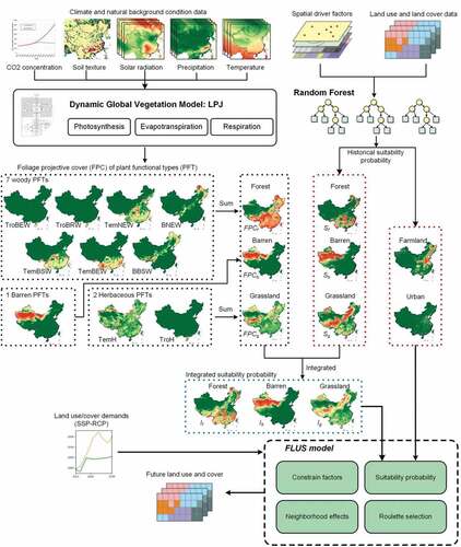
A coupled model, LPJ-FLUS, is proposed by integrating the LPJ and RF-FLUS models (Liu et al. 2017; Zhang et al. 2019). The proposed model is used to simulate five LULC types in China: forest land, grassland, farmland, urban land, and barren land (water area is considered to remain unchanged). The LPJ model is used to calculate the natural vegetation (i.e. forest land, grassland, and barren land) suitability probability, and the RF-FLUS model is used to simulate the future LUCC. Figure 1 displays the flowchart of this research.

Figure 1. Flowchart of this study.

2.1 LPJ model

The LPJ DGVM (Sitch et al. 2003) is a process-based ecosystem model that simulates photosynthesis, evapotranspiration, and respiration of different PFTs by explicitly modeling their plant structure, dynamics, and competition. The model is driven by soil texture, CO₂ concentration, monthly temperature, monthly precipitation, and solar radiation data. Moreover, it can simulate the future geographical distribution of PFTs by inputting the simulated climate data (e.g. data provided by CMIP6) into the model. The LPJ model yields a 0.5° × 0.5° grid of foliage projective cover (FPC), representing the coverage ratio of 10 different PFTs under specific natural conditions.

As shown in Table 1, the PFT types in the LPJ model are correlated to the land types used herein. The FPC of woody PFTs is totaled as the FPC of the forest land. The FPC of herbaceous PFTs is summed as the FPC of grasslands. The remaining fractions of a grid that FPCs do not cover are treated as the proportion of barren land covered. For convenience, it is hereinafter referred to as the FPC of barren land.

Table 1. PFTs modeled by LPJ and their corresponding LULC types.

PFT	LULC types in MODIS	LULC types in this study
Tropical broad-leaved evergreen woody (TroBEW)	Evergreen needleleaf forests	Forest
Tropical broad-leaved raingreen woody (TroBRW)	Evergreen broadleaf forests
Temperate needle-leaved evergreen woody (TemNEW)	Deciduous needleleaf forests
Temperate broad-leaved evergreen woody (TemBEW)	Deciduous broadleaf forests
Temperate broad-leaved summergreen woody (TemBSW)	Mixed forests
Boreal needle-leaved evergreen woody (BNEW)
Boreal broad-leaved summergreen woody (BBSW)
Temperate herbaceous (TemH)	Closed shrublands	Grassland
Tropical herbaceous (TroH)	Woody savannas
	Savannas
	Grasslands
	Permanent wetlands
Barren	Open shrublands	Barren
	Barren or sparsely vegetated
	Snow and ice
-	Urban and built-up lands	Urban
-	Croplands	Farmland
	Cropland/natural vegetation mosaics
-	Water bodies	Water

FPCs reflect the suitability probability of natural vegetation from a mechanistic perspective, because the FPC of PFTs in the LPJ model is determined by the biogeographical, biochemical, and meteorological conditions that determine the occurrence/persistence of vegetation. Therefore, in the LPJ-FLUS model, the FPC of forest land, grassland, and barren land in the target year are used as a proxy of the suitability probability of natural vegetation from a mechanistic perspective to adjust the suitability probability based on machine learning in the CA model.

The 0.5° × 0.5° grid fraction FPC of each PFT outputted by the LPJ model is acquired from the Inter-Sectoral Impact Model Intercomparison Project (Warszawski et al. 2014). The CO₂ concentrations corresponding to the RCP-2.6 and RCP-8.5 scenarios (Moss et al. 2010) are used as input. Future atmospheric climate data are simulated with MIROC5 (Watanabe et al. 2010) due to its relatively high spatial resolution (0.5°), and the data are bias-corrected by EWEMBI (Lange 2018). Finally, the FPC data for the terminal year are resampled at a 1 km × 1 km resolution and input to the LPJ-FLUS model.

2.2 FLUS model

This study employs a modified version of CA, the FLUS model, that requires only one period of land data to assess the suitability probability for different land types (Liu et al. 2017). Different machine learning algorithms have been used to mine the suitability probabilities of land types for the FLUS model. For example, ANNs have been successfully employed for land modeling with reliable accuracy, including in combination with the FLUS model (Liu et al. 2017). However, care is needed to overcome its overfitting potential (Xu, Gao, and Coco 2019).

Furthermore, the RF algorithm is another option for assessing the land suitability probability in the FLUS model. It can process a large number of nonlinear elements and is hard to overfit, which resolves the above defects (Kamusoko and Gamba 2015). Recently, the RF algorithm has been widely used in CA models to simulate LUCC (Chen et al. 2019; Du et al. 2018; Li and Chen 2020; Zhang et al. 2019). Therefore, the RF algorithm can be combined with the FLUS model, called RF-FLUS. This study uses RF-FLUS as part of the integration model.

The RF algorithm is an ensemble learning algorithm that comprises multiple decision trees. It generates different training sample subsets and driving factor subsets to train the decision trees. It aims to create an ensemble of “weak” but varied classifiers and then aggregate their predictions. Therefore, the algorithm can effectively avoid the overfitting problem and has superior prediction ability (Belgiu and Drăguţ 2016).

In RF-FLUS, the suitability probability of each cell can be expressed as follows:

(1) $S_i^k=\frac{I\left(h_m\left(i\right)=k\right)}{M}$(1)

Here, $S_i^k$ expresses the suitability probability of the land type k of a cell $i$. $h_m\left(i\right)$ represents the estimation results returned by a single decision tree m for cell i. I is the discriminant function that equates to 1 if $h_m\left(i\right)=k$; otherwise, it is 0. M denotes the number of decision trees.

To train the RF model, 500000 training samples are collected from the spatial datasets in the initial year using the stratified random sampling method; the samples are evenly distributed across the six land types. The collected samples are divided into 60% training samples, 20% validation samples, and 20% test samples to train the RF algorithm and validate the fitting accuracy. After calibration, 200 decision trees are used to construct the RF algorithm and then calculate the suitability probability of each land type. This procedure is performed using python with the open-source scikit-learn package (Version 0.23) (Pedregosa et al. 2015). In the FLUS model, the Moore neighborhood with a radius of 5 is used to represent the neighborhood interactions.

In addition to the suitability probability, RF-FLUS comprises three more factors: neighborhood effect, restriction, and stochastic factors (Zhang et al. 2019). The neighborhood effect is a fundamental element of the LUCC simulation model based on the CA model. The n × n Moore neighborhood interactions ${\mathrm{\Omega }}_i^k$ for a cell i transforming into category k is expressed as

(2) ${\mathrm{\Omega }}_i^k=\frac{{\sum }_{n^2}Con\left(\mathrm{L}=k\right)}{n^2-1}$(2)

Here, $\mathrm{L}$ denotes the land type of neighborhood cells. $Con$ is the indicator function that is 1 if $\mathrm{L}=k$; otherwise, it is 0. Furthermore, in FLUS models, a constraint factor $C$ exists that restricts the conversion of particular categories (Liu et al. 2017).

The total development probability of cell i transforming into category k is expressed as ${\mathrm{P}}_i^k$ (Eq. 3), which comprises suitability probability, neighborhood interactions, stochastic factors, and restriction in the RF-FLUS model.

(3) $P_i^k=S_i^k\times {\mathrm{\Omega }}_i^k\times \mathrm{C}$(3)

To incorporate the competition of different land types, within each iteration, the target categories of cells are decided by a roulette selection mechanism (Liu et al. 2017). The total development probabilities of the different land types of a cell are normalized based on proportions to sum to 1. The target land type is determined by sampling from a probability distribution constructed by the total development probability of different land types in the roulette selection. In this way, the types with high probability are more likely to develop, while the types with low probability also have development opportunities. Furthermore, urban shrinkage is not simulated herein, and thus, urban cell conversion into other types is restricted.

2.3 LPJ-FLUS model

As the suitability probability of land types is an essential part of the LUCC simulation model, many previous studies have focused on it (Chen, Liu, and Li 2017; Du et al. 2018; He et al. 2018; Liu et al. 2008; Wang et al. 2020; Xu, Gao, and Coco 2019; Zhang et al. 2020). This study proposes the integration of LPJ and RF-FLUS by adjusting the suitability probabilities of forest land, grassland, and barren land calculated by the RF and LPJ models. The suitability probabilities calculated by the LPJ and RF models are summed to jointly determine the integrated suitability probability through the weights. As a simplification, in this study, they are summed to have the same weight, i.e. 0.5. Therefore, the integrated suitability probabilities of natural vegetation can be calculated as follows:

(4) $S_v=S_f+S_g+S_b$(4)

(5) $I_f=0.5S_f+0.5S_v\cdot FP{C}_f$(5)

(6) $I_g=0.5S_g+0.5S_v\cdot FP{C}_g$(6)

(7) $I_b=0.5S_b+0.5S_v\cdot FP{C}_b$(7)

Here, $S_f$, $S_g$, and $S_b$ are the suitability probabilities of forest land, grassland, and barren land calculated by RF algorithms, respectively. $S_v$ represents the sum of the suitability probabilities of the natural LULC estimated by the RF algorithm, i.e. the sum of $S_f$, $S_g$, and $S_b$. $FP{C}_f$, $FP{C}_g$, and $FP{C}_b$ denote the suitability probabilities of forest land, grassland, and barren land estimated by LPJ, respectively. $I_f$, $I_g$, and $I_b$ are the integrated suitability probabilities of forest land, grassland, and barren land, respectively. The suitability probability estimated by the RF and LPJ models equally contribute to the integrated suitability probability. It includes the mathematical relationship mined by the RF algorithm as well as the physical relationship modeled by the LPJ model, and it can reliably simulate the future geographical distribution of natural vegetation (Sitch et al. 2003). The adjusted natural vegetation suitability probability and other suitability probabilities without adjustment are input in the FLUS model to simulate the future LULC patterns.

Additionally, the LPJ-FLUS model retains the feature of controlling the land simulation through land demands. The specific methodology for land demand projection is described later in Section 2.5. The future demand for each land type is projected under the SSP1-RCP2.6 and SSP5-RCP8.5 scenarios and is used as macro controls for the model. The model iterations stop when the land area changes to the target amount.

2.4 Data for land simulations

The historical land use and land cover product of China from the MODIS Land Cover Type Product (MCD12Q1; https://lpdaac.usgs.gov/) in 2001, 2010, and 2015 are used in this study. The initial LULC data included 17 classes. The large number of land types poses a great challenge in the determination of the corresponding driving factor data. Therefore, the data are reclassified into six types (forest land, grassland, farmland, urban land, barren land, and water), similar to previous studies (Li et al. 2017) (Table 1). The overall accuracy of the original MODIS data containing 17 land types is about 70% across the different years (Sulla-Menashe et al. 2019). The accuracy of the land data is expected to improve to some extent after merging into six land types. The spatial driving factors used to build and train the RF algorithm are listed in Table 2, including natural environmental and socio-economic factors that are commonly used in LUCC simulation models (Chen, Li, and Liu 2022; Li et al. 2017). With reference to previous studies on land cover change modeling, drivers such as population, distance to urban centers, and distance to roads are chosen herein to reflect the influence of human activities on the land cover change. Similarly, to reflect the impact of natural conditions on the land cover change, the corresponding drivers in terms of terrain, soil properties, and climatic conditions are selected. All the spatial datasets are resampled to 1 km with the same projection. The soil data are the only spatial driving data with a resolution of 5′ (approximately 10 km at the equator). As the spatial heterogeneity of soils is not as sensitive as the socio-economic development, it is believed that the resampling of the soil data to 1 km for modeling will not have a significant impact (Chen, Li, and Liu 2022; Li et al. 2017).

Table 2. List of spatial driving factors.

Category	Driver	Year	Resolution	Data sources
Human influence	Population	2010	0.5′	LandScan
	Distance to urban centers	2014	1km	ESRI World Cities layer
	Distance to roads	2010	1km	ESRI World Roads layer
Terrain	DEM	2000	0.5′	WorldClim
	Slope
Soil	Workability	2008	5′	Harmonized World Soil Database v 1.2
	Oxygen availability to roots
	Excess salts
	Nutrient availability
Climate	Temperature annual range	2000	0.5′	WorldClim
	Temperature seasonality
	Annual mean temperature
	Precipitation seasonality
	Annual precipitation

2.5 Projections of land demands under different scenarios

The proposed LPJ-FLUS model is used to simulate two LUCC scenarios for the period of 2015–2100 in China. Two different SSP-RCP scenarios are used (O’Neill et al. 2016): SSP1-RCP2.6 and SSP5-RCP8.5. SSP1-RCP2.6 represents a low emission concentration path and corresponds to a sustainable socio-economic development. SSP5-RCP8.5 represents a high emission concentration path, corresponding to the fossil-fueled development scenario (O’Neill et al. 2017).

Land demands that are the termination conditions must be determined before the scenario simulations. In this study, the LUH2 dataset provides projections of China’s land demands under these two scenarios (Eyring et al. 2015). LUH2 is the official land dataset of CMIP6; it integrates the area and distribution of future land use under the SSP-RCP scenario as predicted by several authoritative integrated assessment models (IAMs) (Hurtt et al. 2020). Moreover, 2015 is used as the initial year for the future land simulation, but a gap exists between the area of each land type in the MODIS and LUH2 datasets in 2015. Therefore, the area change rate for each land type in LUH2 is calculated for 2015–2100 and applied to the 2015 MODIS LULC map. Subsequently, the adjusted land demands for China in 2015–2100 under SSP1-RCP2.6 and SSP5-RCP8.5 scenarios for future land simulations are obtained.

2.6 Method of evaluating the accuracy of the model

This study uses Figure of Merit (FoM) as the accuracy metric to evaluate the model’s performance (Pontius et al. 2007), which is believed to be superior to Overall Accuracy and Kappa coefficient (Tong and Feng 2020). FoM is calculated by the cells that change in the simulation process while neglecting the persistent ones to assess the performance of LUCC simulations. It is defined as follows:

(8) $FoM=B/\left(A+B+C+D\right)$(8)

where A represents the number of misses (the observed LULC type has changed but the model simulated it as unchanged), B denotes the number of true hits (the observed LULC type has changed and the model predicted the correct change type). C indicates the number of false hits (the observed LULC type has changed but the model predicted the wrong change type). D represents the number of false alarms (the model predicted a change but the observed LULC type remained unchanged).

3 Results

3.1 Model validation by historical simulation

To validate the proposed LPJ-FLUS model, two historical simulations with different periods are performed. Furthermore, to demonstrate the effectiveness of the proposed model, it is compared to two other advanced CA models: RF-FLUS (Zhang et al. 2019) and ANN-FLUS (Liu et al. 2017). Based on China’s LULC data, both historical simulations take 2001 as the initial year but separately simulate up to 2010 and 2015. While performing these two historical simulations, the integrated suitability probabilities are assessed by combining the suitability probabilities for 2001 evaluated by the RF algorithm and the natural vegetation suitability probabilities for the target years estimated by the LPJ method. Figures 2 and 3 show the actual and simulated LULC patterns in 2010 and 2015 obtained using LPJ-FLUS, RF-FLUS, and ANN-FLUS.

Figure 2. Simulated land use/land cover pattern by LPJ-FLUS, RF-FLUS, and ANN-FLUS for 2010.

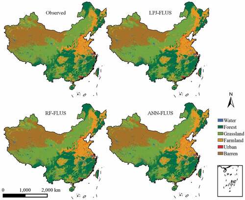
Figure 3. Simulated land use/land cover pattern by LPJ-FLUS, RF-FLUS, and ANN-FLUS for 2015.

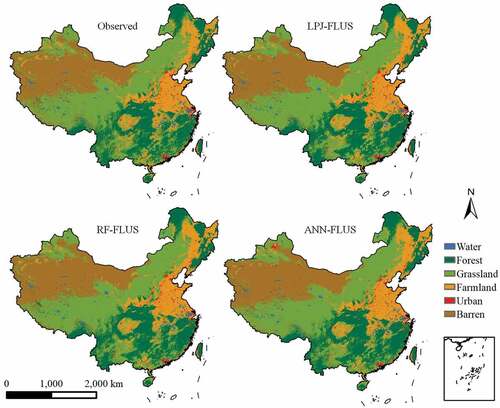
The simulation accuracy is shown in Table 3. The results show that LPJ-FLUS is superior to the other models and exhibits the highest FoM in the two simulated years. Compared to the other two models, the FoM of LPJ-FLUS is higher by 5.14% and 5.71% in 2010 and 2.35% and 2.45% in 2015, which shows that LPJ-FLUS can effectively improve the LUCC accuracy by explicitly integrating the natural vegetation simulation capability of LPJ.

Table 3. Accuracy (FoM) of the simulated results by different models.

Year	LPJ-FLUS	RF-FLUS	ANN-FLUS
2010	23.37%	18.23%	17.66%
2015	16.73%	14.37%	14.28%

The FoM of each land type is illustrated in Table 4. Compared to RF-FLUS and ANN-FLUS, the FoM of grassland in LPJ-FLUS is higher by 4.92%–8.14%, with an average of 6.53%; the FoM of forest land in LPJ-FLUS is higher by 2.51%–6.02%, with an average of 4.18%; the FoM of barren land in LPJ-FLUS is higher by 0.13%–5.54%, with an average of 2.82%; and the FoM of farmland and urban land in LPJ-FLUS is higher by 1.78% and 1.60% on average, respectively. The results indicate that the LPJ-FLUS model significantly improves the simulation accuracy of grassland and forest land, proving the effectiveness of the coupled model.

Table 4. FoM of each land type.

Year		Grassland	Forest	Farmland	Urban	Barren
2010	LPJ-FLUS	21.12%	23.00%	22.89%	7.07%	22.38%
	RF-FLUS	13.79%	17.54%	19.94%	8.05%	18.44%
	ANN-FLUS	12.98%	16.98%	19.77%	7.16%	16.84%
2015	LPJ-FLUS	15.51%	16.48%	15.74%	11.18%	12.98%
	RF-FLUS	10.59%	13.76%	14.88%	9.64%	12.85%
	ANN-FLUS	9.80%	13.97%	15.57%	5.24%	11.31%

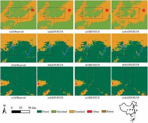
Three typical regions from the simulated results in 2015 are chosen to illustrate the superiority of the proposed model (Figure 4). The natural vegetation distribution simulated by LPJ-FLUS better matches the actual pattern than that simulated by other models. Traditional CA models only use machine learning to estimate the suitability probability of each land type, which is considered a purely mathematical system. LPJ-FLUS integrates DGVM and uses biophysical and biochemical models to determine the suitability probability of natural vegetation (Sitch et al. 2003). Therefore, it can make up for the deficiency of mathematical methods and simulate reliable natural vegetation distributions.

Figure 4. Comparison of simulated patterns of 2015 generated by LPJ-FLUS, RF-FLUS, and ANN-FLUS in China.

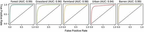
The suitability probabilities estimated by the RF model are crucial for ensuring the accuracy of land simulations. Figure 5 assesses the accuracy of the suitability probabilities estimated by the RF model for each land type using receiver operating characteristic (ROC) curves. Moreover, the area under the curve (AUC) values are used to quantify the accuracy of the suitability probabilities. The results show that the RF model achieves satisfactory accuracy in estimating the suitability probabilities for each land type, achieving AUC values of 0.94 or more.

Figure 5. ROC and AUC of the suitability probabilities for each land cover category estimated by the RF model.

3.2 Future land demands

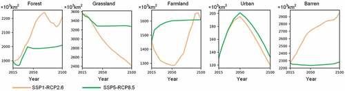
Figure 6 displays the projected land demands for the six land types from 2015 to 2100 for the two scenarios. The areas of each land type exhibit different development trends under the two scenarios, although they commenced with the same initial values in 2015. The SSP-RCP scenarios comprise varying adaptation and mitigation challenges, resulting in different changes in the quantity of each land type under different scenarios (O’Neill et al. 2017; Riahi et al. 2017). In SSP1-RCP2.6, to control global warming, afforestation work is conducted, resulting in a substantial increase in forest land. Furthermore, due to the improved agricultural production efficiency and diet changes, farmland and grassland significantly decrease. With the increase in population, urban land is expected to increase before the 2050s but sharply decrease thereafter since the population is expected to decrease. In SSP5-RCP8.5, forest land slightly increases due to technological progress and human capital development, and farmland and grassland slightly decrease. As the human capital is highly developed, urban land is relatively larger in SSP5-RCP8.5 than that in SSP1-RCP2.6, but it sharply decreases after the 2050s in both scenarios (O’Neill et al. 2017). In this study, at the 1 km scale, it is assumed that the urban grid already allocated will not disappear as its demand decreases.

Figure 6. Projections of forest land, grassland, farmland, urban land, and barren land areas for 2015–2100 under the SSP1-RCP2.6 and SSP5-RCP8.5 scenarios.

3.3 Spatial improvements to the suitability probabilities

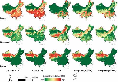
Figure 7 compares the suitability probabilities of forest land, grassland, and barren land estimated by the LPJ model, the RF model, and the proposed LPJ-FLUS. The suitability probability of natural vegetation is quite diverse under different models and climate scenarios. The first two columns of Figure 7 present the suitability probabilities for 2100 under the different scenarios estimated by the LPJ model, which considers different future climate possibilities through mechanistic modeling. The third column of Figure 7 depicts the suitability probabilities assessed by the RF model. They are estimated based on historical and current conditions by mining mathematical laws through machine learning without considering future climate possibilities. The last two columns of Figure 7 are the integrated suitability probabilities generated based on our proposed method. They simultaneously consider historical and current patterns as well as different future climate possibilities by combining the LPJ and RF models. Overall, the LPJ model’s suitability probabilities show that SSP5-RCP8.5 is more suitable for forest development than SSP1-RCP2.6, which may be due to the increased CO₂ fertilization effect caused by higher global warming in SSP5-RCP8.5. Consistent with the scenario setting, the total integrated suitability probability in SSP5-RCP8.5 is 17.93% higher than that in SSP1-RCP2.6. A similar effect is observed in the estimated suitability probability for grassland. The integrated suitability probability of grassland under SSP5-RCP8.5 is 19.26% lower than that under SSP1-RCP2.6, which matches the trend afforded by LPJ model in assessing different future scenarios. Moreover, the RF-estimated suitability probability more accurately reflects the current land cover patterns than the LPJ-estimated suitability probability as it considers finer resolution land cover. However, it cannot reflect the spatial variation in the suitability probability for different future scenarios. Therefore, the integrated suitability probabilities combine the strengths of the RF and LPJ models, providing a better fit with the current LULC pattern and reflecting the conditions in different future scenarios.

Figure 7. Suitability probability of forest land, grassland, and barren land in 2100 under SSP1-RCP2.6 and SSP5-RCP8.5 generated by the LPJ model, the RF model, and LPJ-FLUS.

3.4 Spatial performance of future simulations for natural vegetation

RF-FLUS and LPJ-FLUS are used to simulate the LUCC of China in 2100 under SSP1-RCP2.6 and SSP5-RCP8.5. In the LPJ-FLUS model, the FPC simulated under both scenarios is integrated. The simulation results of LPJ-FLUS better reflect the impact of climate on the spatial distribution of natural vegetation. Compared to RF-FLUS, LPJ-FLUS better simulates the forest land decrease and grassland increase under SSP5-RCP8.5. As the complete maps do not clearly show the patterns, some typical areas are chosen to illustrate the effects of integrating the DGVM. The transition proportion in each 10 km grid is used to represent the land-use dynamics.

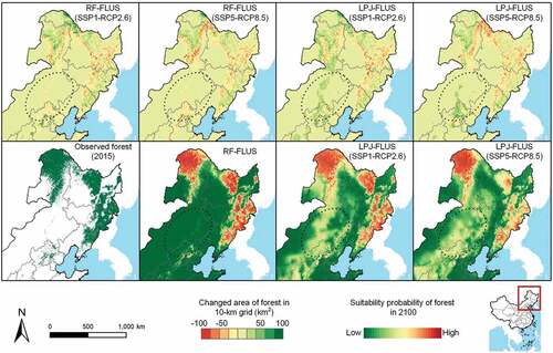
Figure 8 depicts the differences between LPJ-FLUS and RF-FLUS in simulating forest land change from 2015 to 2100 in northeast China, which comprises the largest natural forest region in China. Forest land undergoes a much more significant increase under SSP1-RCP2.6 than that under SSP5-RCP8.5, which is in accordance with the narratives of the two scenarios. Under SSP1-RCP2.6, to mitigate climate change, large-scale afforestation is conducted in northeast China, while under SSP5-RCP8.5, these actions are not performed. LPJ-FLUS simulates more forest growth than RF-FLUS in the western part of the region (i.e. the area circled by the dotted line in Figure 8) due to the various forest suitability probabilities in the different scenarios. Precipitation and temperature variations make this region more suitable for forest development in the future. LPJ-FLUS captures this change by explicitly considering climate change, while RF-FLUS cannot simulate this phenomenon as it is solely based on historical development trends. Thus, the simulation results of LPJ-FLUS are more consistent with the corresponding scenario narratives than those of RF-FLUS.

Figure 8. Differences between LPJ-FLUS and RF-FLUS in simulating forest land change from 2015 to 2100 in northeast China under different scenarios. Top row: transition of forest land from 2015 to 2100. Bottom row: suitability probability of forest land for 2100.

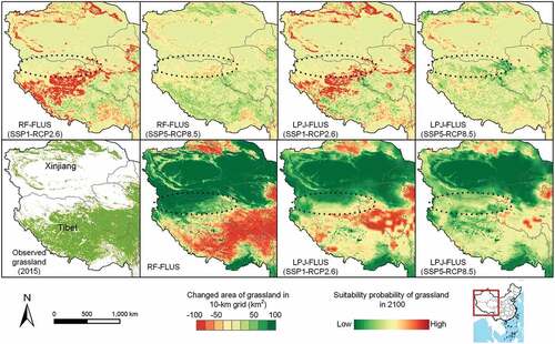
Figure 9 illustrates the differences between the simulation results of the two models in western China’s grassland concentration areas. Most parts of Tibet and the northern part of Xinjiang are two of the most concentrated grassland regions in China. Considerably greater decrease in the grassland area is simulated under SSP1-RCP2.6 than that under SSP5-RCP8.5 in the results of both models. The decrease in the grassland area conforms to the low-meat diets in SSP1-RCP2.6. However, the effectiveness of the LPJ model in guiding spatial changes in grassland is also evident. The LPJ model indicates better grassland suitability in northern Tibet (i.e. the area circled by the dotted line in Figure 9) than the RF model, particularly in SSP5-RCP8.5. Thus, in SSP1-RCP2.6, where the grassland area rapidly decreases, LPJ-FLUS simulates less grassland reduction in northern Tibet relative to RF-FLUS. In SSP5-RCP8.5, the LPJ model exhibits a marked increase in grassland suitability probability in northern Tibet, which does not overlap with its distribution in 2015 but is influenced by the future climate change. Thus, in SSP5-RCP8.5, LPJ-FLUS and RF-FLUS simulate grassland increase and decrease in northern Tibet, respectively.

Figure 9. Differences between LPJ-FLUS and RF-FLUS in simulating grassland change from 2015 to 2100 in western China under different scenarios. Top row: transition of the grassland from 2015 to 2100. Bottom row: suitability probability of grassland for 2100.

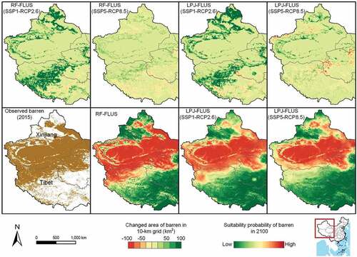
Figure 10 illustrates the difference between the two models in simulating barren land change. The region shown is one of the best-known contiguous areas of barren land in China, with large areas of desert and barren lands. A much greater increase in barren land area is observed under SSP1-RCP2.6 than that under SSP5-RCP8.5. The significant increase in the barren land area is due to the abandonment of grassland stemming from the low-meat diet assumption in SSP1-RCP2.6. LPJ-FLUS simulates more barren land area increase in Xinjiang than in Tibet under the same scenario because the LPJ model guides the reduction of the suitability of barren land in Tibet. Therefore, the simulation results of LPJ-FLUS are more consistent with future climate change and vegetation distribution than those of RF-FLUS.

Figure 10. Differences between LPJ-FLUS and RF-FLUS in simulating barren land change from 2015 to 2100 in western China under different scenarios. Top row: transition of the barren from 2015 to 2100. Bottom row: suitability probability of barren for 2100.

Furthermore, the effect of LPJ-FLUS in considering the spatial distribution of natural vegetation provided by the LPJ model was quantitatively measured. Since the suitability probabilities provided by the LPJ model (i.e. FPC) are integrated at the cell-level into the suitability probabilities of the FLUS model, the spatial distribution of the LPJ-FLUS simulation results is expected to be more relevant to the suitability probabilities provided by the LPJ model than that of the RF-FLUS simulation results. For comparison, the area percentage of each natural vegetation type was separately determined from the FPC and simulation results within each 0.25° grid to obtain the Pearson correlation between the suitability probabilities provided by the LPJ model and the simulation results from the LPJ-FLUS and RF-FLUS models. Table 5 displays the comparison of the correlations. The results show that the simulation results from LPJ-FLUS are more correlated with the distribution of suitability probabilities provided by the LPJ model in all scenarios and natural vegetation types than those from RF-FLUS, with an increase in the Pearson correlation coefficients (R) by 0.03. This demonstrates the effectiveness of the LPJ-FLUS model in integrating the LPJ model to improve spatial simulations. The Pearson correlation coefficient for grassland exhibits a slightly negative value because the LPJ model provides a smaller range of grassland distribution than MODIS. However, the correlation coefficients for grassland in LPJ-FLUS are still more biased toward the LPJ model than those in RF-FLUS.

Table 5. Correlation of the suitability probabilities provided by the LPJ model in 2100 with the simulated spatial distribution of natural vegetation from LPJ-FLUS and RF-FLUS.

	LPJ-FLUS		RF-FLUS
	Land cover	R	Land cover	R
SSP1-RCP2.6	Forest	0.8267**	Forest	0.8141**
	Grassland	−0.0732**	Grassland	−0.0765**
	Barren	0.6478**	Barren	0.6361**
SSP5-RCP8.5	Forest	0.7935**	Forest	0.7764**
	Grassland	−0.0869**	Grassland	−0.1151**
	Barren	0.7101**	Barren	0.6906**

Note: **indicates a significant correlation at the 0.01 level.

4 Discussion

4.1 The performance of the LPJ-FLUS model

To measure the performance of LPJ-FLUS, it is compared with conventional CA models in terms of both historical simulations and future predictions. Validation results from the historical simulations show that LPJ-FLUS can improve the FoM values by up to 5% compared to conventional CA models that do not consider spatial coupling with mechanistic models and by even up to 8% for certain vegetation types. This is attributed to the fact that LPJ-FLUS not only statistically considers the role of spatial drivers on land change but also considers the assessment of the spatial suitability of natural vegetation based on biogeographic and biochemical mechanisms.

Regarding future projections, LPJ-FLUS maintains the conventional CA model’s feature of quantitatively constraining land simulations through the future land demand provided by IAMs. Furthermore, LPJ-FLUS integrates the spatial information provided by the LPJ model on the natural vegetation distribution under different future climate scenarios for driving land simulation, which is significantly different from conventional CA models. Information on the natural vegetation distribution under different future climate scenarios based on biogeographic and biochemical mechanisms is unavailable from machine learning algorithms, which can only mine rules from history. Figures 8–10 demonstrate the advantages of this spatial coupling mechanism. In some places where certain natural vegetation types have not historically existed, the RF algorithm assesses that such places are unsuitable for such natural vegetation. However, the LPJ model may assess such places as being favorable to the growth of such natural vegetation in the future based on changes in the growing conditions due to future climate changes. LPJ-FLUS then integrates this spatial information provided by the LPJ model to simulate changes in the natural vegetation distribution in areas where growing conditions significantly change under future climate scenarios. Furthermore, the Pearson correlation analysis based on grid statistics demonstrates that the spatial distribution of natural vegetation in the simulation results of LPJ-FLUS is closer to that of the LPJ model than RF-FLUS, with an improvement in the correlation coefficient of 0.03. This quantitatively demonstrates the effectiveness of LPJ-FLUS in coupling the LPJ model for the spatial driving of land change.

4.2 The cell-level coupling mechanism

Cell-level model coupling is the distinguishing feature that sets LPJ-FLUS apart from the conventional CA models. Previous mechanistic models have been loosely coupled with CA models. Mechanistic models, such as IAMs and system dynamics models, provide projected land demands as iterative termination constraints for CA models in future land simulations. In contrast, LPJ-FLUS innovatively integrates the land data projected by the mechanistic model into the suitability probabilities of the CA model, thus allowing the mechanistic model to spatially drive land simulations. The spatial presentation and quantitative analysis of the simulation results have demonstrated the effectiveness of this coupling mechanism.

Furthermore, the cell-level coupling mechanism could be more comprehensively explored. In this study, equal weights are simply set on the contribution of the LPJ and RF models to the integrated suitability probability. In the future, the weight setting could be varied. For example, in some scenarios where climate change is more extreme, suitability based on historical mining may play a less important role. Thus, in such cases, the suitability probabilities provided by the LPJ model should contribute more weight.

4.3 Potential applications

Benefiting from the cell-level coupling mechanism, the proposed LPJ-FLUS has the following potential applications. First, it can be used for fine-scale land simulations under extreme climate scenarios as it combines the relatively fine spatial resolution of CA models with the ability of mechanistic models to project LUCC under extreme climate scenarios. Second, it can be used for spatially tight coupling with models of different structures, including but not limited to mechanistic models. Moreover, it can be used to assess the environmental impacts of LUCC under extreme climate scenarios.

4.4 Limitations and future works

Inevitably, this study has some limitations. First, herein, some driving forces have a relatively low spatial resolution, ranging from 5′ to 30′ (approximately 10–55 km on the equator). For example, the spatial resolution of the soil quality dataset used herein is only 5′. As the spatial heterogeneity of the soil quality is relatively small, previous studies have stated that a resolution of 5′ can capture the actual spatial distribution of the soil quality (Li et al. 2017). Limited by the spatial resolution of the climate model (Watanabe et al. 2010), the resolution of FPC grids simulated by the LPJ model is only 30′. However, this resolution is sufficient for capturing the changes in suitability probability under global climate and environmental changes. With the development of the climate model, the spatial resolution of the LPJ model can be further improved to enhance LUCC simulation performance. Second, this study used only the 2100 data from the LPJ model when coupling the provided future natural vegetation suitability probabilities. In the future, when producing long-time series and multi-year future land projection products, the corresponding data of intermediate years provided by the LPJ model could be used for the LUCC simulations to yield more refined spatial information from the mechanistic model. Third, due to limitations of the data availability, the RF model only considers historical drivers in estimating the suitability probabilities. As the projections go further in time, the historical drivers introduce errors. In future studies, with improving data availability, the suitability probabilities estimated by the RF model using the projected future drivers can be updated when conducting future simulations to reduce the errors stemming from the historical data. Fourth, in this study, the natural vegetation suitability probabilities provided by the LPJ and RF models were coupled by simply setting the same weights. However, the optimal weights vary across the regions. In the future, optimization and sensitivity of the weights could be explored. Fifth, the proposed cell-level coupling mechanism proposed herein is only based on the LPJ model. Thus, in the future, how other forms of spatial projection data provided by other mechanistic models can realize spatial coupling with a CA model or even tighter coupling in terms of model structure should be explored. In addition, the proposed LPJ-FLUS can be used for high-resolution and small-scale simulations when fine spatially driving factor data, LPJ data, and sufficient computational resources are available.

5 Conclusion

This study proposed LPJ-FLUS, which integrates a CA model with DGVM. The proposed method can realistically simulate LUCC due to the integration of the natural vegetation grid FPC simulated by LPJ, which comprises biogeographic and biochemical models. It can more reasonably simulate the distribution of natural vegetation than traditional CA models. Previous studies have often loosely coupled mechanistic models with CA models by providing land demands. Herein, the spatial results provided by the mechanistic model were employed to generate the integrated suitability probabilities that directly guide the spatial LULC simulation of the FLUS model at the cell level. In this way, a tighter coupling was achieved between the CA and mechanistic models. This coupling can improve the interpretability of future LUCC simulated by CA models. Comparison of the simulation results with the observations in 2010 and 2015 showed that LPJ-FLUS is superior to the well-accepted ANN-FLUS and RF-FLUS, with FoM value improvement by 5% or even 8% in some natural vegetation types. Furthermore, the future LUCC was simulated under SSP1-RCP2.6 and SSP5-RCP8.5. The integration of the natural vegetation grid FPC of the two scenarios simulated by the LPJ model showed that the LUCC simulated by LPJ-FLUS is more consistent with the scenario narratives and effectively enables the LPJ model to spatially drive land simulations. Furthermore, the proposed LPJ-FLUS provides a new idea for the tight coupling of mechanistic and CA models and will contribute to the LUCC simulation community.

Acknowledgements

This research was supported by the National Science Fund for Distinguished Young Scholars [No. 42225107]; National Natural Science Foundation of China [No. 42171409]; National Natural Science Foundation of China [No. 42171410]; Natural Science Foundation of Guangdong Province of China [No. 2021A1515011192]; Science and Technology Program of Guangzhou, China [No. 202201011149].

Disclosure statement

No potential conflict of interest was reported by the authors.

Data availability statement

The data that support the findings of this study are openly available in figshare at https://figshare.com/s/c31247c33c08b59110f3.

Additional information

Funding

The work was supported by the The National Science Fund for Distinguished Young Scholars .

References

- Belgiu, M., and L. Drăguţ. 2016. “Random Forest in Remote Sensing: A Review of Applications and Future Directions.” ISPRS Journal of Photogrammetry and Remote Sensing 114: 24–18. doi:10.1016/j.isprsjprs.2016.01.011.
- Braakhekke, M. C., J. C. Doelman, P. Baas, C. Müller, S. Schaphoff, E. Stehfest, and D. P. Van Vuuren. 2019. “Modeling Forest Plantations for Carbon Uptake with the LPJmL Dynamic Global Vegetation Model.” Earth System Dynamics 10 (4): 617–630. doi:10.5194/esd-10-617-2019.
- Chen, G., X. Li, and X. Liu. 2022. “Global Land Projection Based on Plant Functional Types with a 1-Km Resolution Under Socio-Climatic Scenarios.” Scientific Data 9 (1): 125. doi:10.1038/s41597-022-01208-6.
- Chen, G., X. Li, X. Liu, Y. Chen, X. Liang, J. Leng, X. Xu, et al. 2020. “Global Projections of Future Urban Land Expansion Under Shared Socioeconomic Pathways.” Nature Communications 11 (1): 537. doi:10.1038/s41467-020-14386-x.
- Chen, Y., X. Li, X. Liu, Y. Zhang, and M. Huang. 2019. “Tele-Connecting China’s Future Urban Growth to Impacts on Ecosystem Services Under the Shared Socioeconomic Pathways.” The Science of the Total Environment 652: 765–779. doi:10.1016/j.scitotenv.2018.10.283.
- Chen, Y., X. Liu, and X. Li. 2017. “Calibrating a Land Parcel Cellular Automaton (LP-CA) for Urban Growth Simulation Based on Ensemble Learning.” International Journal of Geographical Information Science 31 (12): 2480–2504. doi:10.1080/13658816.2017.1367004.
- Chen, G., J. Xie, W. Li, X. Li, L. C. Hay Chung, C. Ren, and X. Liu. 2021. “Future “Local Climate Zone” Spatial Change Simulation in Greater Bay Area Under the Shared Socioeconomic Pathways and Ecological Control Line.” Building and Environment 203: 108077. doi:10.1016/j.buildenv.2021.108077.
- Dietrich, J. P., B. L. Bodirsky, F. Humpenöder, I. Weindl, M. Stevanović, K. Karstens, U. Kreidenweis, et al. 2019. “MAgPie 4 – a Modular Open-Source Framework for Modeling Global Land Systems.” Geoscientific Model Development 12 (4): 1299–1317. doi:10.5194/gmd-12-1299-2019.
- Dietzel, C., and K. C. Clarke. 2007. “Toward Optimal Calibration of the SLEUTH Land Use Change Model.” Transactions in GIS 11 (1): 29–45. doi:10.1111/j.1467-9671.2007.01031.x.
- Doelman, J. C., E. Stehfest, A. Tabeau, H. van Meijl, L. Lassaletta, D. E. H. J. Gernaat, K. Neumann-Hermans, et al. 2018. “Exploring SSP Land-Use Dynamics Using the IMAGE Model: Regional and Gridded Scenarios of Land-Use Change and Land-Based Climate Change Mitigation.” Global Environmental Change 48: 119–135. (December). 2017. 10.1016/j.gloenvcha.2017.11.014.
- Dong, N., L. You, W. Cai, G. Li, and H. Lin. 2018. “Land Use Projections in China Under Global Socioeconomic and Emission Scenarios: Utilizing a Scenario-Based Land-Use Change Assessment Framework.” Global Environmental Change 50: 164–177. doi:10.1016/j.gloenvcha.2018.04.001.
- Du, G., K. J. Shin, L. Yuan, and S. Managi. 2018. “A Comparative Approach to Modelling Multiple Urban Land Use Changes Using Tree-Based Methods and Cellular Automata: The Case of Greater Tokyo Area.” International Journal of Geographical Information Science 32 (4): 757–782. doi:10.1080/13658816.2017.1410550.
- Eyring, V., S. Bony, G. A. Meehl, C. Senior, B. Stevens, R. J. Stouffer, and K. E. Taylor. 2015. “Overview of the Coupled Model Intercomparison Project Phase 6 (CMIP6) Experimental Design and Organisation.” Geoscientific Model Development Discussions 8 (12): 10539–10583. doi:http://doi.org/10.5194/gmdd-8-10539-2015.
- Foley, J. A., R. DeFries, G. P. Asner, C. Barford, G. Bonan, S. R. Carpenter, F. S. Chapin, et al. 2005. “Global Consequences of Land Use.” Science 309 (5734): 570–574. doi:10.1126/science.1111772.
- He, J., X. Li, Y. Yao, Y. Hong, and Z. Jinbao. 2018. “Mining Transition Rules of Cellular Automata for Simulating Urban Expansion by Using the Deep Learning Techniques.” International Journal of Geographical Information Science 32 (10): 2076–2097. doi:10.1080/13658816.2018.1480783.
- Hua, W. J., H. S. Chen, and X. Li. 2015. “Effects of Future Land Use Change on the Regional Climate in China.” Science China Earth Sciences 58 (10): 1840–1848. doi:10.1007/s11430-015-5082-x.
- Hurtt, G. C., L. Chini, R. Sahajpal, S. Frolking, B. L. Bodirsky, K. Calvin, J. C. Doelman, et al. 2020. “Harmonization of Global Land Use Change and Management for the Period 850–2100 (LUH2) for CMIP6.” Geoscientific Model Development 13 (11): 5425–5464. doi:10.5194/gmd-13-5425-2020.
- Kamusoko, C., and J. Gamba. 2015. “Simulating Urban Growth Using a Random Forest-Cellular Automata (RF-CA) Model.” ISPRS International Journal of Geo-Information 4 (2): 447–470. doi:10.3390/ijgi4020447.
- Lange, S. 2018. “Bias Correction of Surface Downwelling Longwave and Shortwave Radiation for the EWEMBI Dataset.” Earth System Dynamics 9 (2): 627–645. doi:10.5194/esd-9-627-2018.
- Li, X., and Y. Chen. 2020. “Projecting the Future Impacts of China’s Cropland Balance Policy on Ecosystem Services Under the Shared Socioeconomic Pathways.” Journal of Cleaner Production 250: 119489. doi:10.1016/j.jclepro.2019.119489.
- Li, X., G. Chen, X. Liu, X. Liang, S. Wang, Y. Chen, F. Pei, and X. Xu. 2017. “A New Global Land-Use and Land-Cover Change Product at a 1-Km Resolution for 2010 to 2100 Based on Human–Environment Interactions.” Annals of the American Association of Geographers 107 (5): 1040–1059. doi:10.1080/24694452.2017.1303357.
- Liu, X., G. Hu, B. Ai, X. Li, G. Tian, Y. Chen, and S. Li. 2018. “Simulating Urban Dynamics in China Using a Gradient Cellular Automata Model Based on S-Shaped Curve Evolution Characteristics.” International Journal of Geographical Information Science 32 (1): 73–101. doi:10.1080/13658816.2017.1376065.
- Liu, X., X. Liang, X. Li, X. Xu, J. Ou, Y. Chen, S. Li, S. Wang, and F. Pei. 2017. “A Future Land Use Simulation Model (FLUS) for Simulating Multiple Land Use Scenarios by Coupling Human and Natural Effects.” Landscape and Urban Planning 168: 94–116. doi:10.1016/j.landurbplan.2017.09.019.
- Liu, X., X. Li, X. Shi, S. Wu, and T. Liu. 2008. “Simulating Complex Urban Development Using Kernel-Based Non-Linear Cellular Automata.” Ecological modelling 211 (1–2): 169–181. doi:10.1016/j.ecolmodel.2007.08.024.
- Liu, H., and Y. Yin. 2013. “Response of Forest Distribution to Past Climate Change: An Insight into Future Predictions.” Chinese Science Bulletin 58 (35): 4426–4436. doi:10.1007/s11434-013-6032-7.
- Li, X., and A. G. O. Yeh. 2002. “Neural-Network-Based Cellular Automata for Simulating Multiple Land Use Changes Using GIS.” International Journal of Geographical Information Science 16 (4): 323–343. doi:10.1080/13658810210137004.
- Moss, R. H., J. A. Edmonds, K. A. Hibbard, M. R. Manning, S. K. Rose, D. P. Van Vuuren, T. R. Carter. 2010. “The Next Generation of Scenarios for Climate Change Research and Assessment.“ Nature 463: 747–756. doi:10.1038/nature08823
- Newbold, T., L. N. Hudson, S. L. L. Hill, S. Contu, I. Lysenko, R. A. Senior, L. Börger, et al. 2015. “Global Effects of Land Use on Local Terrestrial Biodiversity.” Nature 520 (7545): 45–50. doi:10.1038/nature14324.
- O’Neill, B. C., E. Kriegler, K. L. Ebi, E. Kemp-Benedict, K. Riahi, D. S. Rothman, B. J. van Ruijven, et al. 2017. “The Roads Ahead: Narratives for Shared Socioeconomic Pathways Describing World Futures in the 21st Century.” Global Environmental Change 42: 169–180. doi:10.1016/j.gloenvcha.2015.01.004.
- O’Neill, B. C., C. Tebaldi, D. P. van Vuuren, V. Eyring, P. Friedlingstein, G. Hurtt, R. Knutti, et al. 2016. “The Scenario Model Intercomparison Project (ScenarioMip) for CMIP6.” Geoscientific Model Development 9 (9): 3461–3482. doi:10.5194/gmd-9-3461-2016.
- Pedregosa, F., G. Varoquaux, L. Buitinck, G. Louppe, O. Grisel, and A. Mueller. 2015. “Scikit-Learn: Machine Learning in Python.” Journal of Machine Learning Research 19 (1): 29–33. doi:10.1145/2786984.2786995.
- Pontius, R. G., R. Walker, R. Yao-Kumah, E. Arima, S. Aldrich, M. Caldas, and D. Vergara. 2007. “Accuracy Assessment for a Simulation Model of Amazonian Deforestation.” Annals of the Association of American Geographers 97 (4): 677–695. doi:10.1111/j.1467-8306.2007.00577.x.
- Popp, A., F. Humpenöder, I. Weindl, B. L. Bodirsky, M. Bonsch, H. Lotze-Campen, C. Müller, et al. 2014. “Land-Use Protection for Climate Change Mitigation.” Nature Climate Change 4 (12): 1095–1098. doi:10.1038/nclimate2444.
- Riahi, K., D. P. van Vuuren, E. Kriegler, J. Edmonds, B. C. O’Neill, S. Fujimori, N. Bauer, et al. 2017. “The Shared Socioeconomic Pathways and Their Energy, Land Use, and Greenhouse Gas Emissions Implications: An Overview.” Global Environmental Change 42: 153–168. doi:10.1016/j.gloenvcha.2016.05.009.
- Schaphoff, S., M. Forkel, C. Müller, J. Knauer, W. Von Bloh, D. Gerten, J. Jägermeyr, et al. 2018. “LPJmL4 – a Dynamic Global Vegetation Model with Managed Land – Part 2: Model Evaluation.” Geoscientific Model Development 11 (4): 1377–1403. doi:10.5194/gmd-11-1377-2018.
- Seto, K. C., B. Güneralp, and L. R. Hutyra. 2012. “Global Forecasts of Urban Expansion to 2030 and Direct Impacts on Biodiversity and Carbon Pools.” Proceedings of the National Academy of Sciences of the United States of America 109 (40): 16083–16088. doi:10.1073/pnas.1211658109.
- Sitch, S., B. Smith, I. C. Prentice, A. Arneth, A. Bondeau, W. Cramer, J. O. Kaplan, et al. 2003. “Evaluation of Ecosystem Dynamics, Plant Geography and Terrestrial Carbon Cycling in the LPJ Dynamic Global Vegetation Model.” Global Change Biology 9 (2): 161–185. doi:10.1046/j.1365-2486.2003.00569.x.
- Sleeter, B. M., T. L. Sohl, M. A. Bouchard, R. R. Reker, C. E. Soulard, W. Acevedo, G. E. Griffith, et al. 2012. “Scenarios of Land Use and Land Cover Change in the Conterminous United States: Utilizing the Special Report on Emission Scenarios at Ecoregional Scales.” Global Environmental Change 22 (4): 896–914. doi:10.1016/j.gloenvcha.2012.03.008.
- Sohl, T. L., K. L. Sayler, M. A. Drummond, and T. R. Loveland. 2007. “The Fore-Sce Model: A Practical Approach for Projecting Land Cover Change Using Scenario-Based Modeling.” Journal of Land Use Science 2 (2): 103–126. doi:10.1080/17474230701218202.
- Sulla-Menashe, D., J. M. Gray, S. P. Abercrombie, and M. A. Friedl. 2019. “Hierarchical Mapping of Annual Global Land Cover 2001 to Present: The MODIS Collection 6 Land Cover Product.” Remote Sensing of Environment 222: 183–194. doi:10.1016/j.rse.2018.12.013.
- Tang, G., and P. J. Bartlein. 2012. “Modifying a Dynamic Global Vegetation Model for Simulating Large Spatial Scale Land Surface Water Balances.” Hydrology and Earth System Sciences 16 (8): 2547–2565. doi:10.5194/hess-16-2547-2012.
- Tong, X., and Y. Feng. 2020. “A Review of Assessment Methods for Cellular Automata Models of Land-Use Change and Urban Growth.“ International Journal of Geographical Information Science 34: 866–898. doi:10.1080/13658816.2019.1684499
- Tubiello, F. N., M. Salvatore, A. F. Ferrara, J. House, S. Federici, S. Rossi, R. Biancalani, et al. 2015. “The Contribution of Agriculture, Forestry and Other Land Use Activities to Global Warming, 1990-2012.” Global Change Biology 21 (7): 2655–2660. doi:10.1111/gcb.12865.
- Verburg, P. H., W. Soepboer, A. Veldkamp, R. Limpiada, V. Espaldon, and S. S. A. Mastura. 2002. “Modeling the Spatial Dynamics of Regional Land Use: The CLUE-S Model.” Environmental management 30 (3): 391–405. doi:10.1007/s00267-002-2630-x.
- Wang, H., B. Zhang, C. Xia, S. He, and W. Zhang. 2020. “Using a Maximum Entropy Model to Optimize the Stochastic Component of Urban Cellular Automata Models.” International Journal of Geographical Information Science 34 (5): 924–946. doi:10.1080/13658816.2019.1687898.
- Warszawski, L., K. Frieler, V. Huber, F. Piontek, O. Serdeczny, and J. Schewe (2014). The Inter-Sectoral Impact Model Intercomparison Project (ISI–MIP): Project Framework. Proceedings of the National Academy of Sciences, 111(9), 3228–3232.
- Watanabe, M., T. Suzuki, R. O’Ishi, Y. Komuro, S. Watanabe, S. Emori, T. Takemura, et al. 2010. “Improved Climate Simulation by MIROC5: Mean States, Variability, and Climate Sensitivity.” Journal of Climate 23 (23): 6312–6335. doi:10.1175/2010JCLI3679.1.
- Xu, T., J. Gao, and G. Coco. 2019. “Simulation of Urban Expansion via Integrating Artificial Neural Network with Markov Chain–Cellular Automata.” International Journal of Geographical Information Science 33 (10): 1960–1983. doi:10.1080/13658816.2019.1600701.
- Zeng, L., X. Liu, W. Li, J. Ou, Y. Cai, G. Chen, M. Li, G. Li, H. Zhang, and X. Xu. 2022. “Global Simulation of Fine Resolution Land Use/Cover Change and Estimation of Aboveground Biomass Carbon Under the Shared Socioeconomic Pathways.” Journal of environmental management 312: 114943. doi:10.1016/j.jenvman.2022.114943.
- Zhang, Y., X. Liu, G. Chen, and G. Hu. 2020. “Simulation of Urban Expansion Based on Cellular Automata and Maximum Entropy Model.” Science China Earth Sciences 63 (5): 701–712. doi:10.1007/s11430-019-9530-8.
- Zhang, D., X. Liu, X. Wu, Y. Yao, X. Wu, and Y. Chen. 2019. “Multiple Intra-Urban Land Use Simulations and Driving Factors Analysis: A Case Study in Huicheng, China.“ GIScience & Remote Sensing 56: 282–308. doi:10.1080/15481603.2018.1507074.