Revealing the time lag between slope stability and reservoir water fluctuation from InSAR observations and wavelet tools— a case study in Maoergai Reservoir (China)

ABSTRACT

Reservoir water fluctuation in supply and storage cycle have strong triggering effects on landslides on both sides of reservoir banks. Early identification of reservoir landslides and revealing the relationship between slope stability and the triggering factors including reservoir level and rainfall, are of great significance in further protecting nearby residents’ lives and properties. In this paper, based on the small baseline subset time series method (SBAS-InSAR), the potential landslides with active displacements in the river bank of Maoergai hydropower station in Heishui County from 2018 to 2020 were monitored with Sentinel-1 data. As a result, a total of 20 unstable slopes were detected. Subsequently, it was found through a gray correlation analysis that the fluctuation of the reservoir water level is the main triggering factor for the displacement on unstable slopes. This paper applied wavelet tools to quantify the time lag between slope stability and reservoir water fluctuation, revealing that the displacement exhibits a seasonal trend, whose high-frequency signal displacement has an interannual period (1 year). Based on the Cross Wavelet Transform (XWT) analysis, under the interannual scale of one year, the reservoir water fluctuation and nonlinear displacement show a clear common power in wavelet. Additionally, a time lag of 65–120 days between slope stability and reservoir water fluctuations has been found, indicating that the non-linear displacements were behind the water level changes. Among the factors affecting the time lag, the elevation of the points and their distance to the bank shore show Pearson’s correlation coefficients of 0.69 and 0.70, respectively. The observed time lag and correlations could be related to the gradual saturation/drainage processes of the slope and the drainage path. This paper demonstrates the technical support to quantitatively reveal the time lag between slope stability and reservoir water fluctuation by InSAR and wavelet tools, providing strong support for the analysis of the mechanisms of landslides in Maoergai reservoir area.

KEYWORDS:

• Time lag
• SBAS-InSAR
• wavelet tools
• reservoir water fluctuation
• slope stability

1. Introduction

The majority of reservoir landslides are distributed on high and steep slopes on both sides of reservoirs. These landslides are characterized by the difficulty to predict their displacement evolution, intensity, and suddenness, to evaluate their destructive power, as well as to continuously monitor them (Dai et al. 2020; Lu et al. 2019). Previous studies of reservoir bank landslides demonstrated that reservoir’s water storage and supply cycle cause important disturbances on bank stability, resulting in landslides (Shi et al. 2021). The most famous reservoir landslide is the Vajont landslide in Italy, which killed more than 2,000 people in 1963 (Müller-Salzburg 1987). Although on a lesser scale, a large landslide occurred in Qianjiangping in 2003, in the Three Gorges during the reservoir impoundment, killing 24 people and causing major damage (Jian et al. 2014). Other examples of reservoir landslides are the Huangtupo landslide at the Three Gorges, China (Wang, Li, and Du 2022), the Xingguang village landslide at the Xiluodu Reservoir, China (Zhu et al. 2022), the Punatsangchhu-I dam landslide, China (Dini et al. 2020), the Ripponvale in the Clyde Dam reservoir, New Zealand (Macfarlane 2009) and the 1959 event at the Pontesei reservoir (Panizzo et al. 2005), among others. Rainfall is a very well-known landslide trigger in the Three Gorges at the same time (Liu et al. 2021; Kang et al. 2017). Therefore, to detect slopes instabilities in high mountain areas, to analyze the main influencing factors triggering reservoir bank landslides and to quantify the relationship between landslide displacement and triggering factors are of paramount importance for: a) the study of landslide displacement changes; b) local disaster prevention and mitigation; c) triggering factors analysis and d) water conservancy and hydropower stations safety.

For monitoring landslide displacements on the reservoir banks, some traditional geodetic techniques are difficult to implement (e.g. total station) because of the treacherous terrain (Dun et al. 2021). Other techniques, as the use of optical images to identify landslides, present some advantages as for example a high resolution, although its use is constrained by the existence of clouds and fog on the area of interest (Feng et al. 2016). Furthermore, small displacements on landslides cannot be promptly identified and monitored using optical images, which are not conducive to large-scale monitoring either (Zheng 2019). In comparison, Interferometric Synthetic Aperture Radar (InSAR) technology has been successfully used in various landslide studies. InSAR provides a day and night and all-weather imaging capability for measuring ground-surface displacements, has a strong penetration capability and a short revisiting time. Therefore, InSAR can be used not only for landslide displacements monitoring and early warning (Kang et al. 2017; Zhu et al. 2014; Dai et al. 2020; Sun et al. 2015; Dong et al. 2019; Hao et al. 2019) but also for identifying large-scale potential landslides (Dai et al. 2020; Zhang et al. 2018; Liu et al. 2013; Zhang et al. 2018; Dun et al. 2021; Xu, Dong, and Li 2019; Zhang et al. 2021). Consequently, InSAR has been widely used to detect reservoir bank landslides, determining their location, displacements information, landslide activity status, etc. (Dun et al. 2021; Liu et al. 2021; Zhou et al. 2020; Tomás et al. 2016). Most of the studies about reservoir bank landslide displacement characteristics in the Three Gorges revealed that landslide movements exhibit a clear seasonality (Liu et al. 2021).

In China, seasonal movements are highly correlated with rainfall (Hu et al. 2016; Zhao et al. 2012, 2018), especially with heavy rainfalls occurred every summer (Liu et al. 2021), and the time lag between peak rainfall and maximum landslide displacement is about 1–2 months in some previous researches (Zhao et al. 2012, 2018). On the other hand, reservoir water fluctuations are also an important factor, and there is also a correlation between reservoir water fluctuations and seasonal landslide signals (Liu et al. 2013; Michoud et al. 2016). Slope displacement often occurs after water storage (Liu et al. 2021), and under different water storage conditions, these displacement signals exhibit different time lag and sensitivity to water fluctuations (Liu et al. 2013, 2021). Among the available studies, there are multiple qualitative analyses of the relationship between slope instability and influencing factors (e.g. Zhou et al. 2020; Tomás et al. 2016; Reyes-Carmona et al. 2020, 2021). Complementarily, there are multiple methods, as the independent component analysis (ICA), the mean cross-correlation analysis (Chaussard and Farr 2019; Wang et al. 2021; Cohen‐waeber et al. 2018) and the wavelet tools (Tomás et al. 2016; Liu et al. 2021; Kalia 2022), which are used as state-of-the-art effective quantitative approaches to explore the relationship between displacements and influence factors. The above-mentioned studies show that rainfall and water level fluctuation changes have a direct impact on landslide displacement and are important triggering factors for landslides. Therefore, it is of paramount importance to detect stability of the slopes in the reservoir area, to analyze the correlation between displacement and water level fluctuation changes, to explore the relationship between unstable slopes in the reservoir bank area and the triggering factors, as well as quantify the hysteresis of the displacements.

This paper explores the use of the Small Baseline Subset InSAR (SBAS-InSAR) method to detect slope instabilities in the Maoergai reservoir area in Heishui County. Additionally, we perform a statistical correlation analysis between the detected active reservoir instabilities and the triggering factors (i.e. the reservoir water level fluctuation and the rainfall). Finally, we conduct a quantitative analysis of the seasonality, periodicity, and the time lag between the displacement and the main triggering factors using continuous wavelet tools. This study provides key information to support the safe operation of local hydropower stations and a new insight into the study of landslide hysteresis in reservoir bank areas.

2. Study area and data

2.1 Overview of the study area

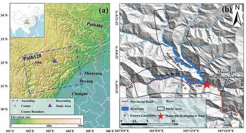
Heishui County is located in the central part of Aba Tibetan and Qiang Autonomous Prefecture in Sichuan Province, east of the Qinghai-Tibet Plateau, with an average elevation of 3,544 m a.s.l. and height differences between 1,000 and 2,000 m. Heishui County presents a typical deep river valley geomorphology. Heishui County is characterized by a monsoonal plateau-type climate, with annual dry and rainy seasons, and is one of the areas in Aba Prefecture with higher accumulated annual precipitations. The average annual rainfall of this area is 620.2 mm, with an uneven rainfall distribution mainly concentrated in summer.

The study area (purple triangle in Figure 1(a)) is crossed by the Heishui, Maoergai and Little Heshui rivers that are dammed by the Maoergai dam (red star in Figure 1(b)). The landform is characterized by deep valleys and high mountains strongly eroded and denudated that lead to steep slopes. This area is dominated by sandstone with unequal-thickness rhyolitic interbeds. These slopes are prone to slope instabilities and are highly conditioned by the long-term erosion caused by the river (Yang et al. 2019). The reservoir impoundment started on 20 March 2011 (Guo, Xu, and Zhao 2015) until a stagnant and a normal water storage level of 2063 and 2133 m a.s.l. was reached, respectively. The reservoir capacity below the normal storage level is 535 million km³. During the rainy season, i.e. between May and October, the stagnant water level gradually rises until reaching the normal water level, maintaining this level during September, December, and April of the next year for water supply (Baidu 2022). On 30 September 2021, a large slope collapsed at the entrance of the Xiergou Tunnel in Heishui County (near Heishui River), causing serious damage to the nearby constructions and posing an important threat to the safety of the nearby roads and people’s lives.

Figure 1. (a) Overview of the study area; and (b) the reservoir area.

2.2 Dataset

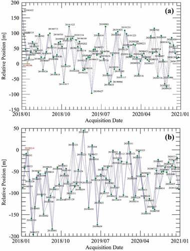
Sentinel-1 satellites, operating in a sun-synchronous orbits with C-band, were launched by the European Space Agency (ESA) to provide continuous worldwide SAR imageries. The Sentinel-1 data used in this work contain νν and νΗ multi-polarizations. A total number of 91 images in ascending orbit and 87 images in descending orbit between 2018 and 2020, spanning 3 years, were used in this study with νν polarization. Since the ascending orbit is more sensitive to east-facing slopes and the descending orbit is more sensitive to west-facing slopes (Dai et al. 2022), the use of both ascending and descending images will considerably improve the capability to detect unstable slopes with different slope aspects. Based on Sentinel-1A images, this paper set a time baseline threshold of 36 days and a spatial baseline threshold of 5% (about 554 m in ascending orbit and 635 m in descending orbit), which enable the generation of 255 interferometric pairs in the ascending orbit and 241 interferometric pairs in the descending orbit (Figure 2).

Figure 2. Spatial and temporal baseline diagrams of interferograms obtained from (a) ascending; and (b) descending images.

3. Methodology

InSAR enables the detection and monitoring of slope displacements of reservoir banks on wide areas. The derived information can be used to qualitatively analyze the existing relationships between the measured displacements and the potential triggering factors based on time-series displacement results. However, these analyses often do not provide quantitative information about the existing relationships. Therefore, this paper quantitatively evaluates the primary and secondary relationships of the influencing factors (i.e. reservoir water fluctuation and rainfall) on the slope displacements detected by SBAS-InSAR technology by means of the gray correlation analysis. Finally, wavelet tools are applied to quantitatively analyze the time–frequency relationships between the non-linear component of InSAR derived displacements of unstable slopes and the above-mentioned triggering factors (Figure 3). The main steps are shown below.

Figure 3. Proposed flow chart for the analysis of InSAR time series of the unstable slopes of Maoergai Reservoir.

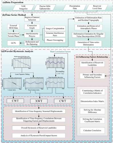
Firstly, the multi-temporal SAR data covering the area of interest were acquired (Figure 3(a)). Then, the coregistration of the images was carried out before the filtering and noise reduction, and the processing was completed by the time-series SBAS-InSAR technology method (Figure 3(b)). Subsequently, the time-series of displacement of the study area based on interferometric pairs with high coherence points were obtained (Zhu, Li, and Hu 2017). According to the time series $t_0,t_1\dots t_N$ a total of N + 1 SLC (Single Look Complex) images were obtained, and one of them was selected as the main image for the coregistration processing with the other images. Consequently, M interferometric pairs were generated by choosing the appropriate spatio-temporal baseline constraint thresholds, the M satisfies,

(1) $\frac{N+1}{2}\le M\le \frac{N\left(N+1\right)}{2}$(1)

where N + 1 shows the number of images acquired.

Then, the orbital information and an external DEM from the shuttle radar topography mission (SRTM) with a resolution of 30 m were used to calculate terrain feature parameters, differentially process each interferometric pair, and remove flatland and topographic effects. The interferometric phase ($\mathrm{\Delta }{\phi }_i\left(x,y\right)$) of each multi-view differential interferogram can be described as,

(2) $\mathrm{\Delta }{\phi }_i\left(x,y\right)=\mathrm{\Delta }{\phi }_{disp}+\mathrm{\Delta }{\phi }_{topo}+\mathrm{\Delta }{\phi }_{atm}+\mathrm{\Delta }{\phi }_{res}$(2)

where $\mathrm{\Delta }{\phi }_{disp}$ is displacement phase along the LOS direction;$\mathrm{\Delta }{\phi }_{topo}$ is terrain phases; $\mathrm{\Delta }{\phi }_{atm}$ is atmospheric phase; and $\mathrm{\Delta }{\phi }_{res}$ is noise phases.

Then, the Minimum Cost Flow (MCF) was used to complete the phase unwrapping (Costantini 1998). After eliminating the interferometric pairs containing phase errors and low coherence, stable ground control points (GCPs) were selected to estimate and remove the residual constant phase and the phase ramp that still existed after unwrapping, to estimate the displacement rate and the residual topography, as well as to perform the atmospheric filtering based on the obtained displacement rate to evaluate and remove the atmospheric phase. Finally, the singular value decomposition (SVD) methods were used to obtain the final displacement rate (Zhou et al. 2017; Li et al., 2021), then the displacement rate results were geocoded based on the external DEM information.

Once the displacement results were obtained by InSAR, the response of the displacement results to the influencing factors was analyzed (Figure 3(c)). The gray correlation was then used to calculate the correlation between the sequence of characteristic variables and the sequence of related factor variables. Furthermore, the order of each influencing factor was derived according to the principle of similarity in the geometry of the sequence curve used to determine the main influencing factor (Dai et al. 2016). First, the gray correlation index matrix, in which each index is dimensionless, was constructed using methods such as initialization and mean-valorization to normalize the values of each index to around 1. Among them, the mean-valorization is more consistent with the characteristics of the time series of the landslide displacement and its influencing factors (Dai et al. 2016). The maximum and minimum values of the absolute difference between the indicator sequence and the reference sequence can be expressed as (Dong and Xie 2016),

(3) $MIN=mi{n}_{i=1}^{n}mi{n}_{j=1}^m\left|y_{ij}-y_{kj}\right|$(3)

(4) $MAX=ma{x}_{i=1}^{n}ma{x}_{j=1}^m\left|y_{ij}-y_{kj}\right|$(4)

where $i$ shows the quantity of influencing factors, $j$ is the quantity of hours, $y_{ij}$ is the reference sequence, $y_{kj}$ is dimensionless matrix;

The gray correlation coefficient matrix can be expressed as follows according to the maximum and minimum values described above,

(5) ${\left[{\xi }_{ij}\right]}_{s\times m}=\frac{MIN+MAX}{\left|y_{ij}-y_{kj}\right|+\eta \times MAX}$(5)

where $\eta$ is resolution coefficient. In order to increase the significance of the differences between the correlation coefficients (Dai et al. 2016), generally $\eta$ = 0.5. The gray correlation is based on the degree of similarity or dissimilarity of the trends between factors to determine the correlation. The correlation between the sequences of influencing factors is expressed as the average of the correlation coefficients at each moment, and the primary and secondary influencing factors are determined according to the size of the average. These formulas are suitable for dynamic analysis in this study. In this paper, the quantity of influencing is three, the quantity of hours is 12, and the monthly cumulative displacements will be used as the reference sequence. The monthly average reservoir levels, and monthly average rainfall will be used as the comparability sequence. The sequences mentioned above are mean-valorization. The purpose of $\eta$ is to improve the variability between the correlation coefficients and is generally taken empirically (Dai et al. 2016).

To analyze the relationship between unstable slope displacements and the main triggering factor, wavelet analysis can be used to reveal the time-frequency features of signals extracted in various time scales, which is a common time-frequency analysis method (Liu et al. 2021). This paper used the Continuous Wavelet Transform (CWT) and Cross Wavelet Transform (XWT) (Figure 3(d)). Before performing the wavelet analysis, the two time series data must be in equal intervals of time, and then interpolation is required if they are not uniform. The time series of the main correlation factor should also be uniformly sampled simultaneously, making the time interval consistent with the InSAR time series results (Figure 3(d)). Wavelet analysis (i.e. CWT, XWT) enables the identification of the periodic displacements described by the non-linear terms of the InSAR time as well as their relationship with the triggering factors (Tomás et al. 2016). Hence, the InSAR time series requires a decomposition of the original InSAR time series, where the linear term is calculated by a linear least-square fit and the nonlinear term is assessed as the difference between the displacement time series and the previously calculated linear component (Liu et al. 2021) (Figure 3(d)). Consequently, wavelet analysis was carried out using a non-linear trend term of the InSAR displacements and the main factors after resampling.

A wavelet is a function, which is limited in both frequency and time with zero average (Grinsted, Moore, and Jevrejeva 2004). The result can be represented as a two-dimensional image over time and frequency and are used to extract the characteristics of the time series. The continuous wavelet transform (CWT) can be thought of as a bandpass filter with different positions and widths (Grinsted, Moore, and Jevrejeva 2004; Vallet et al. 2016; Torrence and Compo 1998), which is expressed as,

(6) $W_x\left(a,b\right)=\underset{-\mathrm{\infty }}{\overset{\mathrm{\infty }}{\int }}x\left(t\right){\psi }_{a,b}^{\ast }\left(t\right)dt$(6)

Where,$a,b$∈R; a≠0, $x\left(t\right)$ is the time series variable, ${\psi }^{\ast }$ is the complex conjugation of $\psi$, a is the scaling factor，and b is the translation factor. In this work, we used Morlet wavelet that is described as $\psi \left(t\right)=e^{\frac{-t^2}{2}}{e}^{i\omega t}$, where $\omega$ is the dimensionless frequency ($\omega$ = 6 can balance time and frequency localization well), and $t$ is the dimensionless time (Grinsted, Moore, and Jevrejeva 2004).

CWT is suitable for time series of limited length, and there may be edge pseudo-effects on the wavelet power spectrum (or scale plot). The edge pseudo-effects will lead to the definition of a cone of influence (COI) in the region where such effects are significant. Besides, the 5% significance level of wavelet power against red noise is shown as a coarse contour on the scale plot. Only patches identified within the thick contours of the COI region can be reliably interpreted (Vallet et al. 2016).

Complementarily, cross wavelet transform (XWT) has been used to identify relationships between common signals of two time series. XWT is the convolution product of the CWT of two time-series. It shows regions with high common power values and its phase represents the time difference between both time-series $x\left(t\right)$ and $y\left(t\right)$. It can be described as (Tomás et al. 2016; Liu et al. 2011),

(7) $W_{xy}\left(a,b\right)=W_x\left(a,b\right)W_y^{\ast }\left(a,b\right)$(7)

where $W_y^{\ast }$ is the complex conjugation of $W_y$ and ${\left|W_x\right|}^2$ is the power of the crossed wavelets. Two signals are identical in time when the arrows face right showing that they are in phase at 0°; when both time-series are inverted the arrows face left indicating that they are in opposite phase at 180°.

The temporal delay or time lag ($\mathrm{\Delta }t$) can be calculated as (Tomás et al. 2020),

(8) $\mathrm{\Delta }\mathrm{t}=\frac{\mathrm{\Delta }\phi \times \mathrm{T}}{2\pi }$(8)

where $\mathrm{\Delta }\phi$ is the arrow angle in radians and $T$ is the periodicity or wave period of interest. Finally, the correlation of the relevant influencing factors was analyzed after calculating the hysteresis of each unstable slope detected by InSAR.

4. Results

4.1 Slope with displacements

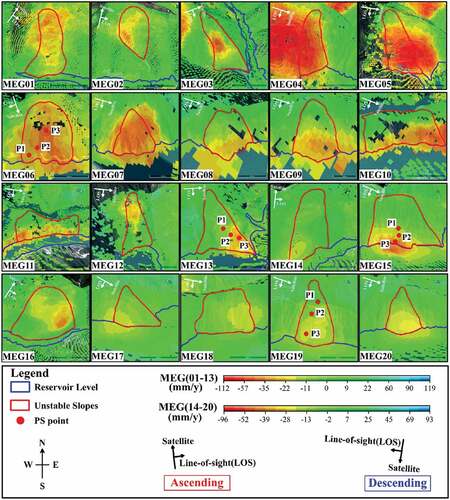
Based on the SBAS-InSAR technique described in section 3, a total of 20 unstable slopes (MEG01–13 are from ascending orbiting results and MEG14–20 are from descending orbiting results) partially submerged beneath the waters of the reservoir were successfully detected in the Maoergai reservoir, (Figure 4) (named MEG01–20, respectively, where MEG is an abbreviation for Maoergai). MEG02, MEG04, MEG05, and MEG09 are the known landslide points in Figure 1(b). It should be noted that yellow and red PS (points) represent significant movements away from the satellite’s line of sight, green PS represent the stable areas.

Figure 4. (a) SBAS-InSAR displacement rate results of the Maoergai reservoir in ascending orbiting; (b)sbas-InSAR displacement rate results of the Maoergai reservoir in descending orbiting; (c) Geometric distortion of the ascending orbiting; (d) Geometric distortion of the descending orbiting.

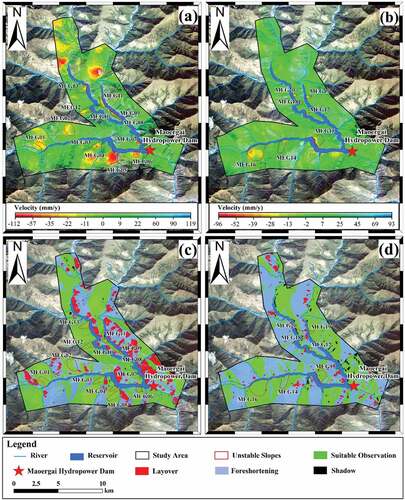
Geometric distortion includes foreshortening, layover, and shadow. Large areas of foreshortening and layover can diminish the visual quality and make interpretation difficult or unreliable, while shadow can render the effective information absolutely invalid and make interpretation impossible. Therefore, the detection results should be as far away from the geometric distortion areas as possible. In Figure 4(c),(d) and Figure 5, the unstable slopes detected by the ascending and descending orbits are located in the suitable observation area, which basically is not affected by geometric distortion, and, consequently, does not affect the interpretation. None of the unstable slopes analyzed are in the regions of geometric distortion, ensuring the reliability of the InSAR monitoring results. The average annual displacement velocity is up to −112 mm/y and up to −96 mm/y for the ascending and descending datasets, respectively. The 20 unstable slopes detected are shown in Figure 5. It is worth noting that the slopes detected on the ascending orbit are all east-facing (MEG01-MEG13), while those detected on the descending orbit are all west-facing (MEG14-MEG20) (Figure 5). The detected unstable slopes are close to the reservoir, providing a good coverage and a high coherence.

Figure 5. Average displacement rate of unstable slopes (MEG01–13 detected in the ascending data and MEG14–20 detected in the descending data).

It should be worth mentioning that the side-view imaging of the radar system has influence on the acquisition of the accurate real-3D displacements. The sensitivity between LOS displacement and slope real displacement is different and is affected by the incidence angle, the slope gradients and the slope aspects among other factors (Dai et al. 2022). In this study, we used ascending and descending data to overcome these drawbacks to some degree regarding on the active slope detection. However, it should be admitted that the LOS displacement acquired in this study are not identical to the real slope displacements. Therefore, their scale factor (system error) would not influence the subsequent correlation analysis between displacements and controlling factors.

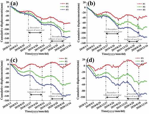
Figure 6 shows the time series of the instabilities MEG06 and MEG13 from the ascending dataset and of MEG15 and MEG19 from the descending dataset. Three PS (P1, P2 and P3, where P1, P2 and P3 exhibit the lower, medium, and higher values of velocity, respectively) exhibiting different displacement rates have been selected on every slope to plot the time-series displacement curves. As can be observed the reservoir unstable slopes exhibit a clear seasonal displacement behavior, showing an obvious cyclical downward trend, with a “step-like” characteristic, and the other unstable slopes have similar trend because of the seasonal rainfall and reservoir water level cycles. Furthermore, it can be seen that all the slopes show an accelerated displacement from December to August every year, which enables to qualitatively state that the unstable slopes present a seasonal periodicity.

Figure 6. Time series displacement curves of landslides (a) MEG06; (b) MEG13; (c) MEG15; and (d) MEG19.

4.2 Main influencing factor analysis

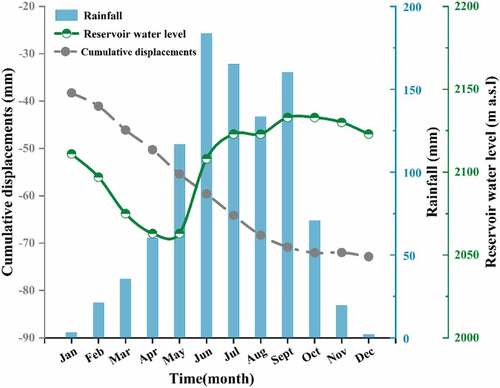
In order to know the relationships between the displacements of the unstable slopes of Maoergai reservoir in Heishui County and its two influencing factors (i.e. rainfall and reservoir water level), 1300 points placed in the unstable slopes of the reservoir bank around the reservoir were selected. The annual average displacement velocity of these points in the ascending orbit is greater than 30 mm/y. Then, the calculated monthly average cumulative displacements, monthly average reservoir levels, and monthly average rainfall of the 3 years are used as the base data (Figure 7).

Figure 7. Yearly relationship between cumulative displacements and influence factors.

The previous data were then used to construct a matrix of gray correlation indicators X=$\left[x_1,x_2,x_3\right]=$[monthly cumulative displacements, monthly rainfall, monthly reservoir water level], and to calculate the correlation coefficient matrix according to Equation (3(3) $MIN=mi{n}_{i=1}^{n}mi{n}_{j=1}^m\left|y_{ij}-y_{kj}\right|$(3) -5(5) ${\left[{\xi }_{ij}\right]}_{s\times m}=\frac{MIN+MAX}{\left|y_{ij}-y_{kj}\right|+\eta \times MAX}$(5) ). 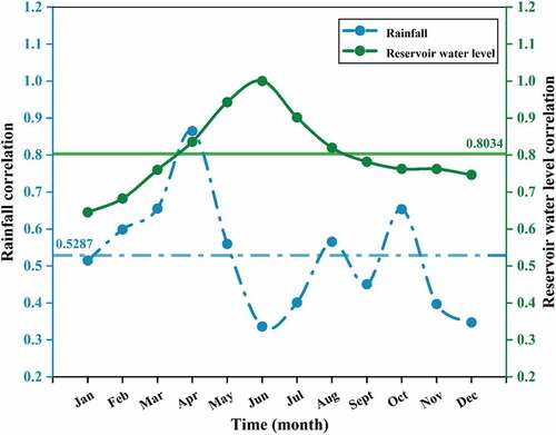Calculating the mean value of correlation coefficient at each time, the correlation degree of correlation factor variable sequences $x_2$ and $x_3$ relative to the reference sequence $x_1$ is r = (0.5287，0.8034) (Figure 8). Figure 8 shows the order of the influencing factors on the cumulative displacement of the unstable slopes in Heishui reservoir bank. Monthly reservoir water level mostly shows higher values than monthly rainfall. The response of unstable slope displacements to monthly reservoir water fluctuations, far exceeds that of rainfall, and its correlation is 0.8034. Therefore, we can conclude that the reservoir water fluctuations are the prime influencing factor controlling the activity of the slopes.

Figure 8. Correlation between cumulative displacements and influencing factors derived from gray correlation analysis.

5. Discussion

5.1 The time lag between the displacements and the reservoir water fluctuations

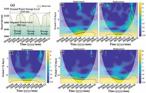
To detect the time–frequency relationships between the reservoir water level and the displacement nonlinear trend of the displacements of the unstable slopes, we used wavelet analysis to decompose the nonlinear trend term from the displacement results detected in subsection 4.1 as one time series and the reservoir water fluctuation as another time series. Both time series were independently used to calculate the CWT.

Figure 9(a) depicts the reservoir water level information after sampling and interpolation. The figure shows that there is a clear seasonal variation and interannual cycle between July and December every year. Figure 9(b)-(f) represent the CWT results for points MEG02, MEG09, MEG13, MEG15, and MEG18, respectively, with peak signals with a period of 24–48 days in July 2018 (Figure 9(c),(d),(f)), August 2019 (Figure 9(b),(d)), and around August 2020 (Figure 9(b)-(f)). Additionally, a strong power is detected during the whole time series for a period of 365 days (i.e. 1 year) that corresponds to the interannual variations of the reservoir water level (Figure 9(b)-(f)). Among all the identified unstable slopes, partial power signals were identified within the August 2018, August 2019 and August 2020, respectively, at the same time the highest reservoir water level were reached in July–December period. This fact indicates a partial response of nonlinear displacements of the unstable slopes to reservoir level changes, showing interannual cycles of about 360 days.

Figure 9. (a) Reservoir water level time series after resampling; (b) CWT of MEG02; (c) CWT of MEG09; (d) CWT of MEG13; (e) CWT of MEG15; (f) CWT of MEG18. 5% significance level relative to red noise is shown as a coarse contour. The wavelets are not fully localized in time and there may be edge pseudo-effects out of the cone of influence (COI).

In order to evaluate the time lag between the overall displacement signal of the reservoir bank and the main triggering factor (i.e. the reservoir water level), the non-linear displacement term from one representative point located in the strongest deformed zone of every unstable slope was selected. Then, XWT was used to identify the common power between both time series. It is worth noting that XWT requires two time-series uniformly sampled, which requires the reservoir water level data corresponding to the ascending/descending orbiting dates.

Figure 10 shows that the arrows are mainly facing down during the 1-year period of significant common power, indicating that the reservoir water fluctuations are ahead of the nonlinear displacements. This fact indicates that the non-linear displacements exhibit a time lag response to the reservoir water fluctuations. To quantify the time lag on interannual structure, we can calculate the specific number of days according to Equation 8(8) $\mathrm{\Delta }\mathrm{t}=\frac{\mathrm{\Delta }\phi \times \mathrm{T}}{2\pi }$(8) . Among the analyzed slopes, MEG02 indicates a time lag about 118 days (arrows in the COI cone and spectral band face downward about 117° to the right, Figure 10(b)) during the 1-year period of significant common power.; MEG09 and MEG13 have a time lag about 102 days (arrows face downward 102°, Figure 10(i), Figure 10(m)); MEG15 and MEG18 both have arrows facing downward 70–75° to the right, with a time lag about 70–75 days (Figures 10(o), 10(r)). The average temporal delay for the interannual cycle is 99.36 days.

Figure 10. Results from cross-wavelet transform (XWT) for the reservoir non-linear displacements with reservoir water level. The black line separates ascending orbiting results (above) from descending orbiting results (below). 5% significance level relative to red noise is shown as a coarse contour. The wavelets are not fully localized in time and there may be edge pseudo-effects out of the cone of influence (COI).

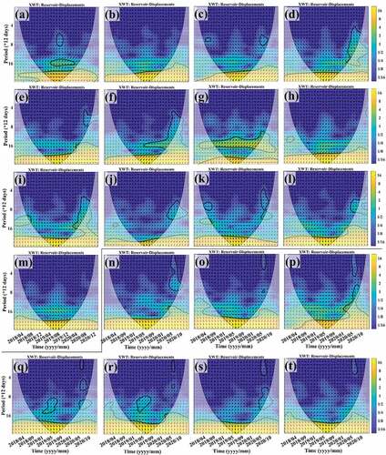
Figure 10 confirms that the reservoir level and the nonlinear displacements time series exhibit a clear high common power over a 365-day (1-year) cycle throughout the study period (2018–2020). Additionally, a few inter-subannual common power signals of 72–120 days and 24–48 days in August 2019 and August 2020 are highlighted, but they are irregularly connected in scale and time. However, the appearance of these structures matches the timing of the high reservoir water level.

Therefore, since the XWT result shows a continuous structure at 1-year period, showing higher power and significant consistency in the annual cycle, only the time lag on the interannual cycle is relatively reliable. In summary, Figure 10 suggests that the nonlinear displacement terms of the 20 unstable slopes have an extremely strong correlation with the reservoir level in the interannual cycle. The arrows in Figure 10 mainly face in the range of 65–120°, indicating that the time series results of the nonlinear displacement trends of the unstable slopes on the banks of the Maoergai present a certain time lag with respect to the reservoir-level fluctuations, which is 65–120 days.

5.2 Factors influencing the time lag

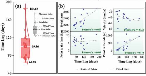
Based on the time lag for each slope, four factors (i.e. elevation of the point, displacement rate of the point, distance of the point along the river to the dam, and distance of the point to the shore) that may affect the length of the time lag period were selected to be analyzed. To this aim, the time lag was plotted against the four factors, and the Pearson’s correlation coefficient was used as a quality indicator for illustrating (Figure 11(b)) the above-mentioned relationships. The Pearson’s correlation coefficients between the time lag and the elevation of the point, the displacement rate of the point, the distance of the point along the river to the dam, and the distance of the point to the shore are 0.69, −0.23, 0.09, and 0.70, respectively (Figure 11(b)). The results show that among these influencing factors, the elevation of the point and the distance of the point from the shore have a relatively high correlation with the time lag. In the other two cases, in which the correlation coefficients are low, indicating that it is unreliable to extrapolate the displacement time lag from the displacement rate of the point (i.e. the velocity) or the distance of the point measured along the river to the dam.

Figure 11. (A) Interannual cycle time lag distribution; (b) time lag and influence factors correlation. The grey dotted lines correspond to the fitted line of each scattered point.

5.3 Reasons analysis of the time lag

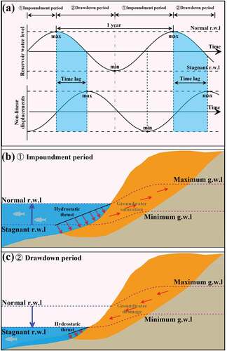
The obtained results above can be explained as follows. The slope gradually rises its groundwater level during the impoundment period saturating the slope and increasing the hydrostatic thrust on the slope surface (Figure 12(b)). The saturation of the slope leads to an increase of the pore water pressure that reduces the effective stress on the soil and the shear strength on the sliding surface. At the same time, the rise of the reservoir water level increases the hydrostatic thrust, which improves the stability of the slope. In contrast, during reservoir water level drawdown periods, the groundwater level within the slope drops and the hydrostatic thrust reduces (Figure 12(c)) (Tomás et al. 2016; Zhou et al. 2016). The combination of both effects (i.e. hydrostatic thrust and slope saturation) mainly control the activity and displacements of the slope. According to Figure 7, when the normal reservoir water level is reached, the slopes exhibit a higher stability (i.e. lower displacements) and vice versa. The hydrostatic thrust acts immediately over the slope after any reservoir water level change. However, the saturation of the slope develops gradually over time since it strongly relies on the permeability of the soil of the slope and the draining path (Figure 12(b) and (c)). This delay between the reservoir impoundment/drawdown and the gradual saturation of the slope could explain the observed delay existing between the reservoir water level and the non-linear component of the displacements that are related to the pore water changes (Figure 12(a)). This explanation is also in agreement with the correlations obtained between the time lag, and the elevation and the distance to the bank river, since the higher the elevation and the distance to the riverbank, the longer the saturating/draining path during the saturation/drainage periods. Furthermore, the non-linear displacements are probably related to consolidation – expansion cycles induced by pore pressure reduction-increase caused by groundwater changes induced by the reservoir water level rise-drawdown (Jiang et al. 2011; Tomás et al. 2014). Consequently, the studied slopes present a continuous displacement (linear component) with minor non-linear cyclic superimposed displacements controlled by the reservoir water level variations.

Figure 12. Conceptual interpretation of the non-linear displacements. a) Time series relationship; b) Impoundment period; c) Drawdown period.

6. Conclusion

Sentinel-1 SAR data covering the period 2018–2020 have been used to detect slope stabilities along the Maoergai reservoir in Heishui County by means of SBAS-InSAR technology. A total of 20 unstable slopes (MEG01–13 are from ascending orbiting results and MEG14–20 are from descending orbiting results) were successfully detected. Monthly precipitations and monthly reservoir water level time series from 2018 to 2020 were also used to find the main influencing factor on the activity of Maoergai reservoir banks. The results derived from gray analysis showed that the influence of reservoir water fluctuation on the slopes was much higher than that of rainfall. Furthermore, wavelet analyses were applied to identify seasonalities by means CWT in the time series, as well to quantify the relationships between the nonlinear displacement trend terms obtained by SBAS-InSAR and the main triggering factor (i.e. the reservoir water level) through the XWT. The results of CWT showed that: a) a partial strong power can be identified throughout the entire analyzed period, indicating that there exist seasonal patterns of unstable slopes nonlinear displacements; b) all nonlinear displacements exhibit an interannual cycle (360 days).

Complementarily, the results of XWT demonstrated that: a) the reservoir water level and the non-linear displacements have a high common power in the interannual cycle (1 year): b) the non-linear displacement changes exhibit a time lag with the reservoir water fluctuations of about 65–120 days; c) the length of the time lag is related to the point elevation and the distance from the point to the shore of the bank. The observed delays can be related to the non-linear displacements caused by pore pressure variations due to the gradual saturation/desaturation process of the slopes and the increase/reduction of the hydrostatic thrust on the submerged part of the landslide after each impoundment/drawdown period, respectively. This study highlights the importance of a close monitoring of the stability of the reservoir bank slopes considering the periodic and hysteresis characteristics of each slope, jointly with an analysis of triggering factors to ensure the operational safety of the reservoir. The method in this study based on the InSAR observations and wavelet tools could be generalization and universal for the time lag analysis in any other reservoir cases. It should be noted that in this study area the unstable slopes are located in a relatively single stratigraphic property (i.e. $T_{3}zh$). Different stratigraphic properties should be taken into account when the stratum is more complex in some cases to ensure the precision of the conclusion.

Disclosure statement

No potential conflict of interest was reported by the author(s).

Data availability statement

All relevant data are available from the authors upon reasonable request. Some datasets that support the findings of this study are available in [https://scihub.copernicus.eu/dhus/#/home], [https://earthexplorer.usgs.gov/], [https://disc.gsfc.nasa.gov/].

Additional information

Funding

The work was supported   by the National Natural Science Foundation of China (Grant No. 41801391), ESA-MOST China DRAGON-5 project (ref. 59339) and the State Key Laboratory of Geohazard Prevention and Geoenvironment Protection Independent Research Project (SKLGP2020Z012) and Sichuan Science Foundation for Outstanding Youth (23NSFJQ0167).

References

- Baidu, W. 2022. “Maoergai Hydropower Station Reservoir Scheduling Regulations.” https://wenku.baidu.com/view/6c4842a4571252d380eb6294dd88d0d232d43c21.html (in Chinese).
- Chaussard, E., and T. G. Farr. 2019. “A New Method for Isolating Elastic from Inelastic Deformation in Aquifer Systems: Application to the San Joaquin Valley, CA.” Geophysical Research Letters 46 (19): 10800–18. doi:10.1029/2019GL084418.
- Cohen‐waeber, J., R. Bürgmann, E. Chaussard, C. Giannico, and A. Ferretti. 2018. “Spatiotemporal Patterns of Precipitation‐modulated Landslide Deformation from Independent Component Analysis of InSar Time Series.” Geophysical Research Letters 45 (4): 1878–1887. doi:10.1002/2017GL075950.
- Costantini, M. 1998. “A Novel Phase Unwrapping Method Based on Network Programming.” IEEE Transactions on Geoscience and Remote Sensing 36 (3): 813–821. doi:10.1109/36.673674.
- Dai, K., J. Deng, Q. Xu, Z. Li, X. Shi, C. Hancock, N. Wen, L. Zhang, and G. Zhuo. 2022. “Interpretation and Sensitivity Analysis of the InSar Line of Sight Displacements in Landslide Measurements.” GIScience & Remote Sensing 59 (1): 1226–1242. doi:10.1080/15481603.2022.2100054.
- Dai, K., Z. Li, Q. Xu, R. Bürgmann, D. G. Milledge, R. Tomas, X. Fan, et al. 2020. “Entering the Era of Earth Observation-Based Landslide Warning Systems: A Novel and Exciting Framework.” IEEE Geoscience and Remote Sensing Magazine 8 (1): 136–153. doi:10.1109/MGRS.2019.2954395.
- Dai, Z., Y. Wei, T. Lv, J. Luo, and W. Yao. 2016. “Deformation Influence Factors of a Landslide in Three Gorges Reservoir Area Based on Grey Correlation Analysis.” The Chinese Journal of Geological Hazard and Control 1: 32–37.
- Dini, B., A. Manconi, S. Loew, and J. Chophel. 2020. “The Punatsangchhu-I Dam Landslide Illuminated by InSar Multitemporal Analyses.” Scientific reports 10 (1): 1–10. doi:10.1038/s41598-020-65192-w.
- Dong, A., and L. Xie. 2016. “A Sensitivity Study on Influencing Factors of Reservoir Landslide Triggers in Three Gorges Reservoir Region—based on Grey Relation Method.” Electronic Journal of Geotechnical Engineering 21.
- Dong, J., L. Zhang, M. Liao, and J. Gong. 2019. “Improved Correction of Seasonal Tropospheric Delay in InSar Observations for Landslide Deformation Monitoring.” Remote Sensing of Environment 233: 111370. doi:10.1016/j.rse.2019.111370.
- Dun, J., W. Feng, X. Yi, G. Zhang, and M. Wu. 2021. “Detection and Mapping of Active Landslides Before Impoundment in the Baihetan Reservoir Area (China) Based on the Time-Series InSar Method.” Remote Sensing 13 (16): 3213. doi:10.3390/rs13163213.
- Feng, Z., B. Li, C. Zhao, L. Wang, and L. Wang. 2016. “Geological Hazards Monitoring and Application in Mountainous Town of Three Gorges Reservoir.” Journal of Geomechanics 22 (3): 685–694.
- Grinsted, A., J. C. Moore, and S. Jevrejeva. 2004. “Application of the Cross Wavelet Transform and Wavelet Coherence to Geophysical Time Series.” Nonlinear Processes in Geophysics 11 (5/6): 561–566. doi:10.5194/npg-11-561-2004.
- Guo, J., M. Xu, and Y. Zhao. 2015. “Study on Reactivation and Deformation Process of XierGuazi Ancient-Landslide in Heishui Reservoir of Southwestern China.” Engineering Geology for Society and Territory-Volume 2: 1135–1141.
- Hao, J., T. Wu, X. Wu, G. Hu, D. Zou, X. Zhu, L. Zhao, R. Li, C. Xie, and J. Ni. 2019. “Investigation of a Small Landslide in the Qinghai-Tibet Plateau by InSar and Absolute Deformation Model.” Remote Sensing 11 (18): 2126. doi:10.3390/rs11182126.
- Hu, X., T. Wang, T. C. Pierson, Z. Lu, J. Kim, and T. H. Cecere. 2016. “Detecting Seasonal Landslide Movement Within the Cascade Landslide Complex (Washington) Using Time-Series SAR Imagery.” Remote Sensing of Environment 187: 49–61. doi:10.1016/j.rse.2016.10.006.
- Jiang, J., D. Ehret, W. Xiang, J. Rohn, L. Huang, S. Yan, and R. Bi. 2011. “Numerical Simulation of Qiaotou Landslide Deformation Caused by Drawdown of the Three Gorges Reservoir, China.” Environmental Earth Sciences 62 (2): 411–419. 10.1007/s12665-010-0536-0
- Jian, W., Q. Xu, H. Yang, and F. Wang. 2014. “Mechanism and Failure Process of Qianjiangping Landslide in the Three Gorges Reservoir, China.” Environmental Earth Sciences 72 (8): 2999–3013. doi:10.1007/s12665-014-3205-x.
- Kalia, A. C. 2022. “Landslide Activity Detection Based on Sentinel-1 PSI Datasets of the Ground Motion Service Germany—the Trittenheim Case Study.” Landslides 20 (1): 1–13. doi:10.1007/s10346-022-01958-9.
- Kang, Y., C. Zhao, Q. Zhang, Z. Lu, and B. Li. 2017. “Application of InSar Techniques to an Analysis of the Guanling Landslide.” Remote Sensing 9 (10): 1046. doi:10.3390/rs9101046.
- Liu, Y., J. Brown, J. Demargne, and D. -J. Seo. 2011. “A Wavelet-Based Approach to Assessing Timing Errors in Hydrologic Predictions.” Journal of Hydrology 397 (3–4): 210–224. doi:10.1016/j.jhydrol.2010.11.040.
- Liu, P., Z. Li, T. Hoey, C. Kincal, J. Zhang, Q. Zeng, and J. -P. Muller. 2013. “Using Advanced InSar Time Series Techniques to Monitor Landslide Movements in Badong of the Three Gorges Region, China.” International Journal of Applied Earth Observation and Geoinformation 21: 253–264. doi:10.1016/j.jag.2011.10.010.
- Liu, Y., H. Qiu, D. Yang, Z. Liu, S. Ma, Y. Pei, J. Zhang, and B. Tang. 2021. “Deformation Responses of Landslides to Seasonal Rainfall Based on InSar and Wavelet Analysis.” Landslides 19 (1): 199–210. doi:10.1007/s10346-021-01785-4.
- Liu, Z., B. Xu, Q. Wang, W. Yu, and Z. Miao. 2021. “Monitoring Landslide Associated with Reservoir Impoundment Using Synthetic Aperture Radar Interferometry: A Case Study of the Yalong Reservoir.” Geodesy and Geodynamics 13 (2): 138–150. doi:10.1016/j.geog.2020.12.001.
- Liu, X., C. Zhao, Q. Zhang, Z. Lu, Z. Li, C. Yang, W. Zhu, J. Liu-Zeng, L. Chen, and C. Liu. 2021. “Integration of Sentinel-1 and ALOS/PALSAR-2 SAR Datasets for Mapping Active Landslides Along the Jinsha River Corridor, China.” Engineering Geology 284: 106033. doi:10.1016/j.enggeo.2021.106033.
- Li, S., W. Xu, and Z. Li. 2021. “Review of the SBAS InSar Time-Series Algorithms, Applications, and Challenges.” Geodesy and Geodynamics 13 (2): 114–126.
- LU, H., W. LI, Q. XU, X. DONG, C. DAI, and D. WANG. 2019. “Early Detection of Landslides in the Upstream and Downstream Areas of the Baige Landslide, the Jinsha River Based on Optical Remote Sensing and InSar Technologies.” Geomatics and Information Science of Wuhan University 44: 1342–1354.
- Macfarlane, D. F. 2009. “Observations and Predictions of the Behaviour of Large, Slow-Moving Landslides in Schist, Clyde Dam Reservoir, New Zealand.” Engineering Geology 109 (1–2): 5–15. doi:10.1016/j.enggeo.2009.02.005.
- Michoud, C., V. Baumann, T. R. Lauknes, I. Penna, M. -H. Derron, and M. Jaboyedoff. 2016. “Large Slope Deformations Detection and Monitoring Along Shores of the Potrerillos Dam Reservoir, Argentina, Based on a Small-Baseline InSar Approach.” Landslides 13 (3): 451–465. doi:10.1007/s10346-015-0583-4.
- Müller-Salzburg, L. 1987. “The Vajont Catastrophe—a Personal Review.” Engineering Geology 24 (1–4): 423–444. doi:10.1016/0013-7952(87)90078-0.
- Panizzo, A., P. De Girolamo, M. Di Risio, A. Maistri, and A. Petaccia. 2005. “Great Landslide Events in Italian Artificial Reservoirs.” Natural Hazards and Earth System Sciences 5 (5): 733–740. doi:10.5194/nhess-5-733-2005.
- Reyes-Carmona, C., A. Barra, J. P. Galve, O. Monserrat, J. V. Pérez-Peña, R. M. Mateos, D. Notti, et al. 2020. “Sentinel-1 DInSar for Monitoring Active Landslides in Critical Infrastructures: The Case of the Rules Reservoir (Southern Spain).” Remote Sensing 12 (5): 809. doi:10.3390/rs12050809.
- Reyes-Carmona, C., J. P. Galve, M. Moreno-Sánchez, A. Riquelme, P. Ruano, A. Millares, T. Teixidó, et al. 2021. “Rapid Characterisation of the Extremely Large Landslide Threatening the Rules Reservoir (Southern Spain).” Landslides 18: 3781–3798. doi:10.1007/s10346-021-01728-z.
- Shi, X., X. Hu, N. Sitar, R. Kayen, S. Qi, H. Jiang, X. Wang, and L. Zhang. 2021. “Hydrological Control Shift from River Level to Rainfall in the Reactivated Guobu Slope Besides the Laxiwa Hydropower Station in China.” Remote sensing of environment 265: 112664. doi:10.1016/j.rse.2021.112664.
- Sun, Q., L. Zhang, X. Ding, J. Hu, Z. Li, and J. Zhu. 2015. “Slope Deformation Prior to Zhouqu, China Landslide from InSar Time Series Analysis.” Remote Sensing of Environment 156: 45–57. doi:10.1016/j.rse.2014.09.029.
- Tomás, R., Z. Li, P. Liu, A. Singleton, T. Hoey, and X. Cheng. 2014. “Spatiotemporal Characteristics of the Huangtupo Landslide in the Three Gorges Region (China) Constrained by Radar Interferometry.” Geophysical Journal International 197 (1): 213–232. doi:10.1093/gji/ggu017.
- Tomás, R., Z. Li, J. M. Lopez-Sanchez, P. Liu, and A. Singleton. 2016. “Using Wavelet Tools to Analyse Seasonal Variations from InSar Time-Series Data: A Case Study of the Huangtupo Landslide.” Landslides 13 (3): 437–450. doi:10.1007/s10346-015-0589-y.
- Tomás, R., J. L. Pastor, M. Béjar-Pizarro, R. Bonì, P. Ezquerro, J. A. Fernández-Merodo, C. Guardiola-Albert, et al. 2020. “Wavelet Analysis of Land Subsidence Time-Series: Madrid Tertiary Aquifer Case Study.” Proceedings of the International Association of Hydrological Sciences 382: 353–359. doi:10.5194/piahs-382-353-2020.
- Torrence, C., and G. P. Compo. 1998. “A Practical Guide to Wavelet Analysis.” Bulletin of the American Meteorological Society 79 (1): 61–78. doi:10.1175/1520-0477(1998)079<0061:APGTWA>2.0.CO;2.
- Vallet, A., J. Charlier, O. Fabbri, C. Bertrand, N. Carry, and J. Mudry. 2016. “Functioning and Precipitation-Displacement Modelling of Rainfall-Induced Deep-Seated Landslides Subject to Creep Deformation.” Landslides 13 (4): 653–670. doi:10.1007/s10346-015-0592-3.
- Wang, S., D. Li, and W. Du. 2022. “Recent Advances in the Investigation of a Slow‐moving Landslide in the Three Gorges Reservoir Area, China.” River 1 (1): 91–103. doi:10.1002/rvr2.8.
- Wang, B., C. Zhao, Q. Zhang, Z. Lu, and A. Pepe. 2021. “Long-Term Continuously Updated Deformation Time Series from Multisensor InSar in Xi’an, China from 2007 to 2021.” IEEE Journal of Selected Topics in Applied Earth Observations and Remote Sensing 14: 7297–7309. doi:10.1109/JSTARS.2021.3096996.
- Xu, Q., X. Dong, and W. Li. 2019. “Integrated Space-Air-Ground Early Detection, Monitoring and Warning System for Potential Catastrophic Geohazards.” Geomatics and Information Science of Wuhan University 44: 957–966.
- Yang, Y., X. Wang, W. Jin, J. Cao, B. Cheng, and S. Zhou 2019. “Characteristics Analysis of the Reservoir Landslides Base on Unmanned Aerial Vehicle (UAV) Scanning Technology at the Maoergai Hydropower Station, Southwest China.” In Proceedings of IOP Conference Series: Earth and Environmental Science,The Second International Workshop on Environment and Geoscience, 17-19 July, Hangzhou, China 349(1), 012009.
- Zhang, L., K. Dai, J. Deng, D. Ge, R. Liang, W. Li, and Q. Xu. 2021. “Identifying Potential Landslides by Stacking-InSar in Southwestern China and Its Performance Comparison with SBAS-InSar.” Remote Sensing 13 (18): 3662. doi:10.3390/rs13183662.
- Zhang, Y., X. Meng, C. Jordan, A. Novellino, T. Dijkstra, and G. Chen. 2018. “Investigating Slow-Moving Landslides in the Zhouqu Region of China Using InSar Time Series.” Landslides 15 (7): 1299–1315. doi:10.1007/s10346-018-0954-8.
- Zhao, C., Y. Kang, Q. Zhang, Z. Lu, and B. Li. 2018. “Landslide Identification and Monitoring Along the Jinsha River Catchment (Wudongde Reservoir Area), China, Using the InSar Method.” Remote Sensing 10 (7): 993. doi:10.3390/rs10070993.
- Zhao, C., Z. Lu, Q. Zhang, and J. de La Fuente. 2012. “Large-Area Landslide Detection and Monitoring with ALOS/PALSAR Imagery Data Over Northern California and Southern Oregon, USA.” Remote Sensing of Environment 124: 348–359. doi:10.1016/j.rse.2012.05.025.
- Zheng, Y. 2019. “Application and Research of InSAR Technology in Three Gorges Reservoir area Landslide Measurement.” Master Degree. China University of Geosciences (Beijing).
- Zhou, C., Y. Cao, K. Yin, Y. Wang, X. Shi, F. Catani, and B. Ahmed. 2020. “Landslide Characterization Applying Sentinel-1 Images and InSar Technique: The Muyubao Landslide in the Three Gorges Reservoir Area, China.” Remote Sensing 12 (20): 3385. doi:10.3390/rs12203385.
- Zhou, L., J. Guo, J. Hu, J. Li, Y. Xu, Y. Pan, and M. Shi. 2017. “Wuhan Surface Subsidence Analysis in 2015–2016 Based on Sentinel-1a Data by SBAS-inSar.” Remote Sensing 9 (10): 982. doi:10.3390/rs9100982.
- Zhou, J., F. Xu, X. Yang, Y. Yang, and P. Lu. 2016. “Comprehensive Analyses of the Initiation and Landslide-Generated Wave Processes of the 24 June 2015 Hongyanzi Landslide at the Three Gorges Reservoir, China.” Landslides 13 (3): 589–601. doi:10.1007/s10346-016-0704-8.
- Zhu, J., Z. Li, and J. Hu. 2017. “Research Progress and Methods of InSar for Deformation Monitoring.” Acta Geodaetica et Cartographica Sinica 46: 1717–1733.
- Zhu, Y., X. Yao, L. Yao, Z. Zhou, K. Ren, L. Li, C. Yao, and Z. Gu. 2022. “Identifying the Mechanism of Toppling Deformation by InSar : A Case Study in Xiluodu Reservoir, Jinsha River.” Landslides 19 (10): 2311–2327. doi:10.1007/s10346-022-01908-5.
- Zhu, W., Q. Zhang, X. Ding, C. Zhao, C. Yang, F. Qu, and W. Qu. 2014. “Landslide Monitoring Byrmation Caused by Drawdown of the Th Combining of CR-InSar and GPS Techniques.” Advances in Space Research 53 (3): 430–439. doi:10.1016/j.asr.2013.12.003.