Spatiotemporal patterns of planted forests on the Loess Plateau between 1986 and 2021 based on Landsat NDVI time-series analysis

ABSTRACT

Long-term and large scale spatiotemporal patterns of planted forests are essential for evaluating local plantation effectiveness and to promote sustainable afforestation. Satellite remote sensing data provide broad spatial coverage and increasingly long-term and large scale records for spatiotemporal analysis of planted forests. In this study, we developed a dynamic and conversion extraction (DCE) framework by combining the similarity of Landsat normalized difference vegetation index (NDVI) time-series with a change detection algorithm. This framework allows the analysis of spatiotemporal dynamics of planted forests. The proposed framework can be used to extract the planting year and conversion patterns of planted forests by performing the Mann-Kendall (MK) statistic test on the inter-annual Landsat NDVI time-series and measuring the similarity of the intra-annual time-series, respectively. Therefore, it can be applied to addressing the key questions on where, when, and how planted forests conversions have occurred. Took the Loess Plateau in China as an example, we applied the DCE framework to illustrate how planted forests have changed over time and space and have been converted from other land cover types from 1986 to 2021. The producer and user accuracies for the mapping of planted forests were 88.22% and 87.11% in 2021, respectively, and the accuracy of identifying planted forests conversions was 80.25%. The results showed that the newly planted forests experienced four phases: a slow rise from 1986 to 2000, a sharp increase during 2001–2004, a fluctuating pattern from 2005 to 2013, and a reduction until 2020, resulting in a total planted forest area of 7.13 Mha in 2021. In addition, 83.51% of the planted forest pixels underwent conversion from grasslands (58.19% or 4.15 Mha) or croplands (25.32% or 1.81 Mha) during 1986–2021. These results indicate the capability of the DCE framework to capture essential information (planting year and conversion patterns) to support the spatiotemporal analysis of planted forests at large scales.

KEYWORDS:

• Change detection
• dynamics and conversion extraction (DCE) framework
• Landsat NDVI time-series
• planted forests
• spatiotemporal patterns
• the Loess Plateau

Introduction

Planted forests, defined as trees or shrubs established through planting or deliberate seeding primarily for ecological purpose (FAO 2020; FRA 2020), play a crucial role in promoting water and soil conservation, delivering eco-social services, and restoring the ecological functions of landscapes (Spracklen and Spracklen 2021), especially in the semi-arid areas (Wang et al. 2020). Over the past decades, numerous forests have been planted worldwide (Chen et al. 2019, 2017). The Chinese government has implemented numerous ecological projects on the Loess Plateau, a typical ecologically fragile ecozone, through afforestation and natural forest protection (Tian et al. 2021; Wang et al. 2020). Characteristic of the spatiotemporal dynamics of planted forests expansion should provide the historical change processes of extent time and long-term pre- and post-afforestation conversion information, other than planted forests area alone (Wang et al. 2020; Griffiths et al. 2014; Carlson et al. 2013), because the ecological services resemble different remarkably between the natural and the planted forests (Hua et al. 2022). However, the spatiotemporal dynamics of planted forests in the semiarid area have not been comprehensively investigated, due partly to the low survival rate of the planted forests. It is reported that less than half of the planted forests survived in the Shelter Forest System Programme in Three-North Regions of China (Wang et al. 2020), and only 15% of total planted forests in the arid and semiarid areas of the northern China survived since 1949 (Cao 2008). The low survival rate of the planted forests makes it impossible to derived the distribution of the extant planted forests from the department’s statistical documents on plantation. Meanwhile, the field surveys are time-consuming and labor-intensive, and dependent heavily on the accessibility, remoteness, and ownership of forests (Hemmerling, Pflugmacher, and Hostert 2021).

Satellite remote sensing data have been extensively used for the continuous monitoring of planted forests dynamics, owing to its broad spatial coverage and increasingly long-term records that largely overlaps with forest projects implements (Xi et al. 2021; Ji et al. 2021; Fagan et al. 2018). Remotely sensed planted forests mapping approaches are the necessary fundament of spatiotemporal patterns analysis, which can be roughly divided into three groups. The first group of approaches utilizes the discrete separability characteristics of planted forests (Duarte, Silva, and Teodoro 2018; Mohajane et al. 2017), such as the multispectral, structural, and temporal features, to characterize plantations that involve a simple change process (Fagan et al. 2018; Dias et al. 2020; Fassnacht et al. 2016). It is applicable for the commercial monoculture forests, as they have relatively high growth rates and short harvest rotation periods. The second group integrate the time-series change detection because disturbance and trends in time-series can be useful for monitoring afforestation (Hemmerling, Pflugmacher, and Hostert 2021). Attributes of planted forests such as location, area, change time, growth conditions and trends can be observed after judging abrupt changes in the time-series of forest pixels (Pasquarella, Holden, and Woodcock 2018). However, this is ineffective when natural forests are disturbed, while planted forests usually grow without abrupt changes unless the land cover type changes (Bey and Meyfroidt 2021). The third group of approaches uses a matching function between the vegetation index (VI) time-series, which considers the complexity of planted forest changes. The images are classified by testing whether the VI time-series of planted forests matches the baseline time-series within a special period, such as the harvesting and planting stages of industrial plantations (Fagan et al. 2018; le Maire et al. 2014; Qiu et al. 2017). Such approaches are widely applied in moderate spatial resolution images (e.g. MODIS), but fail to map planted forests with small patches due to the coarse spatial resolution (le Maire et al. 2014; Deng et al. 2020). The current planted forests mapping approaches provide the fundament for the analysis of the spatiotemporal patterns of planted forests with accurate and detailed spatial information in restoration regions. Information on the extent, time, and trend of afforestation and deforestation are always widely investigated but the knowledge on the spatiotemporally explicit dynamics of planted forest is still lack, especially across large areas and with sufficient spatiotemporal details (Griffiths et al. 2014; Fagan et al. 2018; Yu et al. 2020). Otherwise, the spectral signature of planted forests can vary obviously depending on several factors such as the growth phase, implementation timing of ecological engineering, and consequences of disturbance. Such changes that result in considerable spatial variability remains challenge in analyzing the spatiotemporal dynamics of planted forests (Wang et al. 2020).

In this study, we developed a dynamics and conversion extraction (DCE) framework for the analysis of the spatiotemporal patterns of planted forests with multiple subtypes. As planted forests grow and their canopy coverage increases after the plantation, the normalized difference vegetation index (NDVI) (Rouse et al. 1973) of newly planted forests in subsequent years are slightly higher than those of the preceding year (in the growing seasons) and grows continuously in the subsequent years; meanwhile, the NDVI values fluctuate seasonally within each year. By contrast, NDVI values for other vegetation types only showed the seasonal fluctuations (Kim et al. 2020; Bey and Meyfroidt 2021; Duarte, Teodoro, and Goncalves 2014). Based on the NDVI curves in different land cover types, the DCE framework combines the similarity of Landsat NDVI time-series with a change detection algorithm. We further took the Loess Plateau in China as an example to apply the DCE frame to explore the spatiotemporal dynamics of the planted forests from 1986 to 2021. Specifically, we are to answer three key questions: (1) Where are the planted forests distributed at present; (2) When has the forest been planted (planting year); (3) How the land conversed to the planted forests, i.e. on which land cover types (land previously covered by grassland, cropland, or non-vegetation) have the trees been planted?

Materials and methods

2.1 Study area

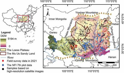
The Loess Plateau is located in North China and covers approximately 64 Mha (Figure 1), with a latitudinal range of 34°–40° N in latitude and a longitudinal range of 102°–114° E in longitude. Geographically, the Loess Plateau is composed of the Liupan, Ziwuling, and Huanglong Mountains from west to east, the Mu Us Sandy Land in the northwest, and the Guanzhong Basin in the south. The climate is characterized by arid and semiarid, with an annual precipitation less than 500 mm, and annual potential evaporation greater than 1,000 mm (Zhang et al. 2013). Natural forests are scarce, and planted forests have a low survival rate owing to inferior soil and climate conditions of arid and semiarid regions (Wang et al. 2020). The Loess Plateau has been subjected to severe soil erosion due to the arid climate, sparse vegetation cover, and a long history of intensive agricultural activity (Liang et al. 2015).

Figure 1. Location of the Loess Plateau and the spatial distribution of the reference samples.

2.2 Construction of the DCE framework

The DCE framework was designed to address the key questions on where, when, and how planted forests conversions with the purpose of providing an insightful view of the spatiotemporal dynamics of planted forests. The proposed DCE framework comprises three key components (i.e. standard NDVI time-series construction, planted forests mapping, and planting year and conversion pattern extraction; see sub-section 2.2.2–4 for more details) and was implemented on the Google Earth Engine (GEE) platform (Gorelick et al. 2017).

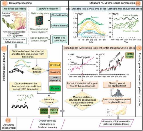
We first constructed the standard NDVI time-series of different land cover types. Considering the intra-class variability among land cover types, we clustered the NDVI time-series reference samples to construct different groups of standard time-series. After that, we calculated the Euclidean distance (ED), i.e. the dissimilarity, between the observed NDVI time-series of one pixel and the standard NDVI time-series of each group of land cover types (Lhermitte et al. 2011; Guo et al. 2020). We then measured the time-series dissimilarity of different land cover types for planted forests mapping as the second key component in the DCE framework. Third, the planting year was detected by performing the Mann-Kendall (MK) statistics test on the inter-annual NDVI time-series. To extract conversion patterns of planted forests, the distance between the observed and standard intra-annual time-series was measured one year prior to the planting year. There are five major steps in our approach: (i) data pre-processing, (ii) standard NDVI time-series construction, (iii) planted forest mapping, (iv) planting year and conversion pattern extraction, and (v) accuracy assessment (Figure 2).

Figure 2. Flowchart of the DCE framework for extracting planting year and conversion patterns of planted forests: (i) data pre-processing, (ii) standard NDVI time-series construction, (iii) planted forest mapping, (iv) planting year and conversion patterns extraction, and (v) accuracy assessment.

2.2.1 Data processing

2.2.1.1 Landsat time-series processing

All available Landsat 5/7/8 surface reflectance data from 1986 to 2021 were used on the GEE platform (Roy et al. 2014; Souverijns et al. 2020). The Landsat archive was corrected to a Level-1 product after systematizing the atmospheric and terrain corrections (Yang and Huang 2021). The Landsat sensors was harmonized to ensure consistency on the GEE platform (Roy et al. 2016)(Roy et al. 2016, available at https://developers.google.com/earth-engine/tutorials/community/landsat-etm-to-oli-harmonization). The CFmask algorithm was used to maintain pixels with less than 30% unclear observations (i.e. clouds and shadows) in an image (Zhu, Woodcock, and Olofsson 2012). Figure A1 shows the number of pixels that are adequately observed each year. The NDVI, an efficient index for examining vegetation growth and forest dynamics (Pan et al. 2018), was calculated using the image collection of all available Landsat 5/7/8 surface reflectance data after removing unclear observations from 1986 to 2021. Intra-annual time-series of NDVI were reconstructed using the harmonic analysis of time-series (HANTS) algorithm, which incorporates both seasonal variations and characteristics to accurately determine periodic changes in vegetation over time (Sellers et al. 1996). The intra-annual time-series was also reconstructed for each year. To compute the similarity expediently, 12 monthly composites was created as the intra-annual NDVI time-series using the maximum reflectance values of the HANTS. Then, inter-annual NDVI time-series were constructed using 36 yearly composites with minimal cloud cover, using the max reflectance values for the growing season, i.e. from April 1- September 30, from the Landsat collection.

2.2.1.2 Field sampling data collection

The forest type cannot be fully detected in the high-resolution image. So firstly, the locations of planted forests (1,265 points) and natural forests (265 points) were designed with the help of the software LocaSpace Viewer (http://uatwww.locaspace.cn/) on the Loess Plateau, and then investigated in July and August 2021. We also derived the land cover type and forest origins information from the Seventh National Forest Inventory (NFI 7th) surveyed from 2004 to 2008. The position errors of the Global Navigation Satellite System (GNSS) coordinates of the NFI 7th plot data were less than 15 m, according to NFI Technical Regulations (Hou et al. 2013). After selecting planted and natural forests by evaluating the forest origin from the NFI 7th data, we determined the forest plots in the Landsat and Google Earth images in 2021. After removing non-forest pixels, 305 planted forest and 2,065 natural forest points were labeled.

2.2.1.3 Reference data collection based on images

We visually identified the other land cover types via most recent Landsat and Google Earth images, which has proven to be a satisfactory and accurate method in determining samples (Ji et al. 2021; Olofsson et al. 2014).

In total, we utilized 7750 pixels as samples for training and validation purposes in this study (Figure 2 and Table 1), including 1,530 points of different forest types from the field survey in 2021, 2,370 from the NFI 7th plot data, and 3,850 points of other land cover types from more recent Landsat and Google Earth images. The reference data collection was then split using a stratified random sampling with 80% samples allocated for training and the remaining 20% for validation by each land cover class (Muchoney and Strahler 2002).

Table 1. Numbers of samples and their sources for each land cover type.

Land cover types		Field survey data	7^th National Forest Inventory	Image data		Total number
Vegetation	Planted forests	1265	305	0	1570
	Natural forests	265	2065	0	2330
	Cropland	0	0	1200	1200
	Grassland	0	0	980	980
Non-vegetation	Bare area	0	0	720	720
	Built-up	0	0	670	670
	Waterbody	0	0	280	280
Total number		1530	2370	3850	7750

2.2.2 Standard NDVI time-series construction

The standard time-series attempted to represent planted forest information and maximally distinguished planted forests from other possible interference landcover types. NDVI time-series of training samples were classified into different categories based on the temporal similarity of each landcover type, and the NDVI time-series of these categories were used as the standard time-series to represent the characteristics of that landcover type. Owing to the variability within each land cover type, the NDVI time-series could display different shapes among land cover types. For example, planted forests start growing from the implementation year in the inter-annual time-series, whereas croplands have one or two peaks within the growing season in the intra-annual time-series. Because there are several groups of time-series for each land cover type, we clustered the NDVI time-series to automatically capture the comprehensive characteristics of different land cover types in the intra-annual and inter-annual time-series as was done by Guo et al. (2020). The intra-annual time-series that represents phenology can provide differentiable information to identify forests and other land cover types; therefore, groups of standard intra-annual time-series were generated as forest, cropland, grassland, and non-vegetation. Subsequently, groups of standard inter-annual time-series were generated to separate planted forests from natural forests. We clustered the time-series of training sample sets to construct different groups of standard time-series in each land cover type using X-means (Pelleg and Moore 2000), an unsupervised clustering algorithm useful for when the classes are unknown in a dataset (Aneece and Thenkabail 2021). The X-means algorithm can automatically determine the optimal cluster size for the input data and is robust to local extrema (Wilson, Knight, and McRoberts 2018; Pelleg and Moore 1999). After every 2-means run, local decisions on whether to split subsets of the current centroid were made.

2.2.3 Planted forests mapping

To analyze the spatiotemporal dynamics of planted forests in the ecological project areas, it is critical to map planted forests accurately. We classified planted forest based on similarity measurements ideal for a long time-series (Qiu et al. 2017). Different land cover types showed different shapes of NDVI curves, because the ground objects were inconsistent. Therefore, we calculated the Euclidean distance (ED_j, Equation 1(1) $EDj=\sqrt{\sum _{i=1}^n{\left(NDV{I}_i-NDV{I}_{ij}^{standard}\right)}^2}$(1) ) between the observed NDVI time-series of each pixel and the standard NDVI time-series of different landcover types (Yan et al. 2019). For each pixel, the ED_j was calculated for both intra-annual and inter-annual time series of NDVI.

(1) $EDj=\sqrt{\sum _{i=1}^n{\left(NDV{I}_i-NDV{I}_{ij}^{standard}\right)}^2}$(1)

where NDVI_i represents of the _ith period (year or month) in the observed NDVI time-series derived from Landsat imagery, n is the length of the NDVI time-series (n = 36 for the inter-annual ED_j and 12 for the intra-annual ED_j, respectively), $NDV{I}_{ij}^{standard}$ represents the _ith period (year or month) of the _jth landcover in the standard NDVI time-series constructed in section 2.2.2.

The minimum distance method was performed to map the planted forests based on the ED_j. The intra-annual ED_j was employed to separate forest from other land cover types, while the inter-annual ED_j was applied to separate planted forests from natural forests. All pixels were classified into different types according to the intra-annual ED_j; each pixel was categorized as the landcover type (forest, cropland, grassland or non-vegetated) with the smallest ED_j. The inter-annual ED_j were further applied to separate planted forests from natural forests. Similarly, all forest pixels were further classified into natural and planted forests according to their inter-annual ED_j with these two types, with distance to the standard inter-annual time-series of planted forests was smaller than that of natural forests were classified as planted forest pixels (Figure 2).

2.2.4 Planting year and conversion pattern extraction

We extracted the planting year and conversion patterns using a time-series detection algorithm, which can determine when and where land cover conversion occurred over the years (Gomez, White, and Wulder 2016). We assumed that the time-series of planted forests increases significantly after planting. We then detected the time when the increasing trend began and assumed it as the planting year of planted forests. The ED_j between the observed and standard intra-annual time-series was calculated one year prior to the planting year to determine on which land cover types have the trees been planted.

The planting year was detected by performing the Mann-Kendall (MK) statistic test (Mann 1945; Kendall 1975) on the inter-annual NDVI time-series. The MK statistic test is a rank-based non-parametric test, and has been widely employed to determine the change in time and duration of significant trends (Some’e, Ezani, and Tabari 2012). It does not require a certain distribution of data and is unaffected by outliers (Fan et al. 2017). Statistically, a series of sequential statistical variables, UF(t), are derived from the MK statistic test. In this study, we used the UF(t) series to detect the planting year and change trends of the NDVI time-series. Changes at a given period were considered significant when UF(t) exceeded the thresholds (i.e. Uα = ± 1.96, 95% significance level); specifically, a UF(t)>1.96 indicates a significant increasing trend in the original data, whilst a UF(t) < −1.96 indicates a decreasing trend, at the 95% significance level.

2.2.5 Accuracy assessment

Validation samples were randomly generated using 20% (i.e. 1,550 pixels) of the sampled pixels. To assess the accuracy of the classification results for 2021, we created a confusion matrix and estimated the overall accuracy, user’s and producer’s accuracy for each class following the procedures defined by Congalton and Green (1993) and Foody (2002) (Foody 2002; Congalton and Green 1993).

The accuracy of the converted planted forests was evaluated by visually examining all 36 yearly composite Landsat images and high-resolution Google Earth imagery to further interpret the pre-land cover types. After determining and recording whether and from which land cover type the planted forests were converted at the validation sample pixels (314 pixels for planted forests), we calculated the conversion accuracy (CA) of the planted forests as Equation 2(2) $CA=\frac{Nc}{Nv}$(2) :

(2) $CA=\frac{Nc}{Nv}$(2)

where Nc indicates the number of correct pixels in the conversion patterns, and Nv indicates the number of validation samples of the planted forests.

2.3 Spatiotemporal patterns analysis

We analyzed the spatiotemporal patterns of planted forests on the Loess Plateau after extracting planting year and conversion patterns to illustrate the changes in planted forests and conversion from other land cover types during 1986–2021. Based on the land cover type before conversion, there were three conversion patterns: persistence (planted forests remained unchanged); afforestation, which can be subdivided into returning croplands to forests (from croplands to planted forests), planting trees on grasslands (from grasslands to planted forests), and afforestation from non-vegetation (from non-vegetation to planted forests); and deforestation, including agricultural expansion (from forests to croplands) and woody clearing (from forests to non-vegetation). The spatiotemporal analysis was implemented in ArcGIS (Esri 2001).

Results

3.1 Accuracy assessment for the DCE framework

The accuracy assessment for the land cover classification in 2021 indicated that the producer and user accuracies were 88.22% and 87.11% for planted forests and 93.99% and 97.55% for natural forests, respectively. Most importantly, the overall accuracy and kappa coefficient reached 92.32% and 0.90, respectively, indicating good performance of the planted forest classification method (Table 2).

Table 2. Accuracy assessment for the land cover classification in 2021.

	Planted forests	Natural forests	Crop-land	Grass-land	Non- vegetation
User accuracy (%)	87.11	97.55	83.20	89.10	99.68	Overall accuracy = 92.32%
Producer accuracy (%)	88.22	93.99	88.75	95.92	94.33	Kappa = 0.90

Accuracy assessments for change detection in the conversion patterns indicated that 80.25% of the planted forest conversions were correctly identified. The MK statistic test did not detect 7.96% of the conversion patterns, whereas 5.41% and 4.14% of the errors originated from the confusion of grasslands and croplands before converting to planted forests, respectively (Table 3).

Table 3. Accuracy assessments for change detection in the conversion patterns types.

Detection types of the conversion patterns
	Correctly identified	Undetected	Changed from cropland misclassified as grassland	Changed from grassland misclassified as cropland	Others	Total
Num of identified pixels	252	25	17	13	7	314
Percentage	80.25%	7.96%	5.41%	4.14%	2.23%	100%
CA = 80.25%

3.2 Spatial pattern of planted forests in 2021

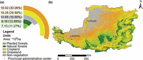
Planted and natural forests occupied 11.27% (7.13 Mha) and 12.9% (8.16 Mha) of the study area, respectively (Figure 3a). Grasslands occupied the largest areas (19.02 Mha; 30.06%), followed by croplands (18.28 Mha; 28.89%), and non-vegetation areas (10.68 Mha or 16.89%). Natural forests mainly concentrated in mountainous regions, such as the Liupan, Ziwuling, Huanglong, Taihang, and Qinling Mountains. Non-vegetation areas were distributed in the desert, mainly in the northwestern part of the Loess Plateau, while grasslands spread to the southeast in the steppe zone. Croplands were widely distributed in the basin, mainly in the Guanzhong Basin and Shanxi Province. Planted forests were mostly densely distributed in the hilly regions in the southeastern part of the Loess Plateau, as well as in the areas between the natural forests and croplands (Figure 3).

Figure 3. Land cover classification results: (a) area (*10⁶ha) and percentage of each land cover type in the study area, and (b) land cover map in 2021.

3.3 Temporal characteristics of planted forest conversion

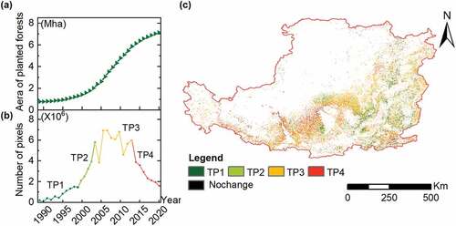
The temporal characteristics of planted forests were determined according to their planting year and conversion during 1986–2021 (Figure 4). The area of total planted forests and number of newly planted forest pixels showed that forest planting underwent four temporal phases (TPs) over time (Figure 4a,b). There was a slow rising trend from 1986 to 2000 (TP1), which resulted in 1.42 Mha of planted forests in 2000 compared to 0.76 Mha in 1986. The area of the afforestation increased sharply since 2000 (TP2), reaching 2.38 Mha in 2004 (Figure 4b). The conversions of TP1 and TP2 were widely distributed in Shanxi Province and central Shaanxi Province (Figure 4c). The area where the land cover changed to planted forests fluctuated and reached a maximum from 2005 to 2013 (TP3), resulting in 5.87 Mha (82% of planted forests) in 2013, widely occurred in Shanxi, western Gansu Province, and central Shaanxi Province. The number of converted pixels decreased until 2020 (TP4), resulting in 7.13 Mha of planted forests in 2021, mostly distributed in the Liupan mountain district of Ningxia and eastern Gansu Province (Figure 4c).

Figure 4. Temporal characteristics of the conversion to planted forests: (a) total area of planted forests and (b) number of newly planted forest pixels in each year forming four temporal phases (TPs), and (c) spatial distribution of the newly planted forests in TP1, TP2, TP3, and TP4, respectively.

3.4 Conversion patterns of planted forests

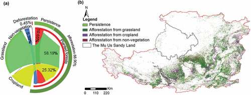
From 1986 to 2021, 88.9% of the planted forests were conversed from other land cover types (Figure 5a). Planting trees on grasslands accounted for the greatest proportion of conversions during this period (58.19% or 4.15 Mha), followed by returning croplands to forests (25.32% or 1.81 Mha). Afforestation from non-vegetation areas accounted for 5.39% (0.39 Mha). Of the planted forest area in 2021, 10.65% (0.76 Mha) were persistent planted forests, i.e. remaining unchanged. However, deforestation (conversion of forests to other landcover types) occurred during the study period, albeit accounting for only 0.45% of all conversions, and most (0.34%) occurred as a result of agricultural expansion. Persistence of planted forests mainly occurred in the southeast of the Loess Plateau, whereas afforestation from non-vegetation occurred in the central Loess Plateau near the Mu Us Sandy Land (Figure 5b).

Figure 5. Conversion patterns of planted forests (i.e. from previous land cover type to planted forests, including persistence, afforestation, and deforestation): (a) chord diagram of conversion patterns, (b) spatial distribution of conversion patterns.

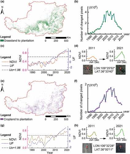
We further illustrated the conversion patterns of afforestation from grasslands and croplands (Figure 6). Previous grasslands were distributed in relatively dry areas of the central Loess Plateau, such as Shanxi Province, and western Gansu Province (Figure 6a). The TPs of afforestation from grasslands, the prominent source of the conversions, were consistent with the temporal characteristics of all conversions to planted forests (Figure 6b). Croplands, the second-largest conversion source, were converted to planted forests in Shanxi Province and central Shaanxi Province (Figure 6e), which went through similar TPs (Figure 6f). The conversion processes of the planted forests are shown in Figures 6c–h from grasslands and croplands, respectively. Inter-annual NDVI time-series and trends in MK statistics (UF) showed that the planting year was 2012, and the intra-annual NDVI time-series of one year prior to the planting year indicated grasslands and croplands converted to planted forests.

Figure 6. Conversion patterns for planting trees on grasslands (a–d) and returning croplands to forests (e–h), (a) spatial distribution of the grasslands converted to planted forests, (b) newly planted forest pixels from grasslands in each year, (c) inter-annual NDVI time-series and trend in MK statistics (UF) of a conversion process from grasslands to planted forests, (d) intra-annual NDVI time-series and corresponding Google Earth image in 2011 and 2021, and (e) spatial distribution of the croplands converted to planted forests, (f) newly planted forest pixels from croplands in each year, (g) inter-annual NDVI time-series and trend in MK statistics (UF) of a conversion process from croplands to planted forests, and (h) intra-annual NDVI time-series and corresponding Google Earth image in 2011 and 2021.

4 Discussion

The DCE framework enhances the extraction effectiveness of the spatial distribution and planting year of planted forests, and reveals the dynamics of planted forests by quantifying conversion patterns. The DCE framework with respect to analyzing the spatiotemporal dynamics of planted forests was performed with high accuracy and robustness.

4.1 Advantages of the DCE framework

Among various strategies implemented by the Chinese government to restore the ecological environment, the Grain to Green Program (GTGP) initiated in 1999 is one of the best known (Chen et al. 2015; Feng et al. 2013). Under the GTGP and the numerous corresponding landscape engineering works such as terracing, check dams, and reservoir construction, the spectral similarity among different vegetation types and spectral variability within the planted forests remain a significant challenge in extracting characteristics planted forests (Yu et al. 2020; Wang et al. 2020). To verify the basis of the DCE, we constructed the inter-annual and intra-annual NDVI time-series of all land cover types based on the training samples (Figures A2 and A3). The long-term NDVI time-series of planted forests showed significantly increasing trends, while natural forests remained stable (Figures A2a,b). Within a year, the planted and natural forests exhibited similar seasonal variation in NDVI (Figures A3a,b). All these observations were consistent with our hypothesis. The intra-annual NDVI time-series was employed to distinguish planted forests from croplands (Figures A3a–c), because some croplands resembled planted forests in the inter-annual NDVI time-series (Figures A2a–c). The similarity of the NDVI time-series contributed to identifying the land cover type to determine the conversion patterns, which remedied a limitation in the current change analysis of planted forests (Yan et al. 2019).

Change detection effectively defines land cover change, but the results may differ depending on the varying time-series algorithms and the magnitude of change (Zhu 2017; Li et al. 2019). We defined planting year in the DCE framework based on significantly increasing trends detected by the MK statistic test at the 95% significance level, which is consistent with the conversion of planted forests (the undetected change accounted for 7.96%). The large increases in TP2 and TP3 are supported by certain previous studies that reported a significant increase in the planted forests coverage since 2000, with a sharp rise after 2005 owing to the implementation of the GTGP (Zhang et al. 2013; Fu et al. 2017; Feng et al. 2016). In addition, the two major sources of planted forests, grasslands and croplands, are in accordance with the finding that grasslands, croplands, and forests were the dominant land cover types of conversion patterns for afforestation in previously studied on the Loess Plateau (Fu et al. 2017).

Our results indicate that the DCE framework can capture key characteristics of NDVI time-series and historical knowledge (planting year and conversion patterns) to support spatiotemporal analysis of planted forests. Importantly, our approach does not attempt to transfer reference sample features that are susceptible to multispectral index, canopy texture, or phenological variations, but relied on automatically generating standard time-series of various land cover types, which is more robust and transferable. Considering the characteristics of different land cover types in groups of time-series (Figures A2 and A3), we can minimize the dependence on spatiotemporally sufficient decisive and historical samples on a large scale. This addresses a challenging aspect of the accurate classification of multi-temporal remote sensing datasets (Amani et al. 2019; Ghorbanian et al. 2020; Tong et al. 2020). The DCE framework for extracting spatiotemporal patterns of planted forests can also serve as a suitable reference for extracting characteristics of planted forest in other parts of the world, as it has the potential to obtain standard time-series with relatively high accuracy and completeness to describe the complex spatiotemporal patterns of planted forests automatically.

4.2 Uncertainties, limitations, and suggestions for future research

The uncertainties include the bias between the planting year extracted in DCE and the planting date on the ground. Planted seedlings are too young to show identifiable spectral signatures; therefore, they can be identified after several years based on the Landsat time-series (Li et al. 2022). On the other hand, the underlying assumption for the characteristics of inter-annual and intra-annual NDVI time-series of planted forests to be stable and robust; however, uncertainties can arise from sensor inconsistencies, varied phenology, and agricultural level differences. The differences in observation frequency may also affect the extraction of the spatiotemporal patterns. Too many missing observations in the growing season may lead to uncertainties in the planting years of forests. The application of multi-source remote sensing data may be an alternative approach to reduce uncertainty (Ling et al. 2022). In this study, we focused on extracting the planting year and conversion patterns of the existing planted forests. In the future, we may use the dynamic windows of time-series as a similarity measure to explore the historical change track of planted forests that have been converted more than once from other land cover types (e.g. the process of grasslands to planted forests, to non-vegetation, and then to planted forests). Additionally, planted forests have changed drastically with respect to time and space on the Loess Plateau over the past 36 years. Further studies on the optimal pattern of planted forests for ecological restoration are important.

5 Conclusion

We developed a DCE framework for analyzing the spatiotemporal dynamics of planted forests on the Loess Plateau over the last 36 years. Results showed that newly planted forests experienced a slow rise from 1986 to 1999, sharply increasing since 2000, fluctuated and reached their maximum between 2005 and 2013, and finally their increase slowly reduced until 2020, resulting in a total area of 7.13 Mha in 2021 on the Loess Plateau. We also found that afforestation from grasslands (58.19%) and croplands (25.32%) were the two major conversion patterns of planted forests during 1986–2021. The DCE framework is suitable for analyzing spatiotemporal dynamics and conversion patterns of ecologically planted forests and can act as a remedy to overcome the limitations in existing change analyze of planted forests. The DCE framework can also serve as a reference for planted forests analysis in other parts of the world, as it has the potential to automatically obtain standard time series with high accuracy. This framework can further integrate spatiotemporal dynamics into forest restoration management and ecosystem service assessment of planted forests to facilitate an evidence-based decision-making process.

Acknowledgments

We thank the Google Earth Engine platform for providing the geospatial datasets and the data processing and analysis algorithms.

Disclosure statement

No potential conflict of interest was reported by the authors.

Data availability statement

The land cover map in 2021 and the core code for clustering standard NDVI time-series and mapping planted forests are available on the Google Earth Engine platform at the following website, respectively (https://code.earthengine.google.com/?asset=users/mengyy225/landcovermapofLoessPlateau; https://code.earthengine.google.com/80f9d3af9b63b2bd2444e33e8ba57bef?asset=users%2Fmengyy225%2FlandcovermapofLoessPlateau; https://code.earthengine.google.com/25331e665bb971836265b92cedac11a6?asset=users%2Fmengyy225%2FlandcovermapofLoessPlateau).

Additional information

Funding

The work was supported by the National Key Research and Development Program of China [2019YFA0606602]; National Natural Science Foundation of China [32025025, 31988102, U1910207]

Appendix Appendix A.

Supplementary data

Figure A1. Number of Landsat observations in each year.

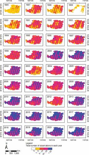
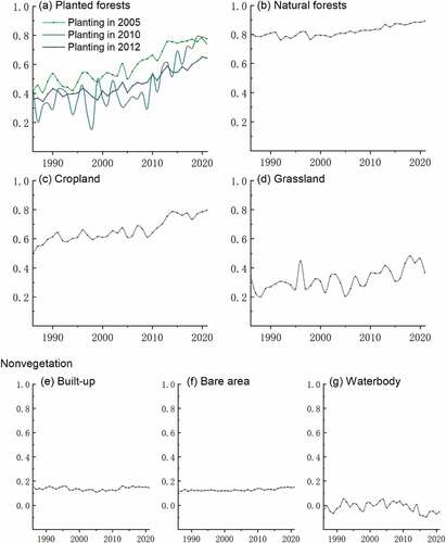
Figure A2. Typical standard inter-annual NDVI time-series for seven land cover types: (a) planted forests, (b) natural forests, (c) cropland, (d) grassland, (e) built-up, (f) bare area, and (g) waterbody.

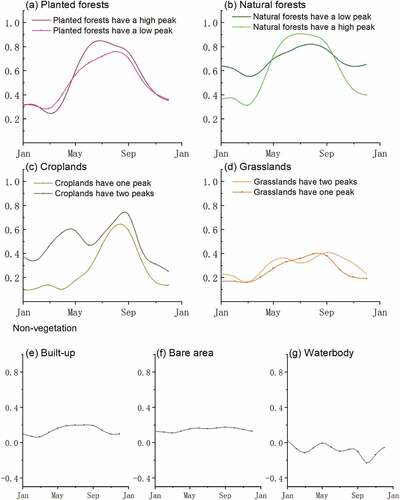
Figure A3. Typical standard intra-annual NDVI time-series for seven land cover types: (a) planted forests, (b) natural forest, (c) cropland, (d) grassland, (e) built-up, (f) bare area, and (g) waterbody.

References

- Amani, M., B. Brisco, M. Afshar, S. M. Mirmazloumi, S. Mahdavi, S. M. Mirzadeh, W. Huang, and J. Granger. 2019. “A Generalized Supervised Classification Scheme to Produce Provincial Wetland Inventory Maps: An Application of Google Earth Engine for Big Geo Data Processing.” Big Earth Data 3 (4): 378–18. doi:10.1080/20964471.2019.1690404.
- Aneece, I., and P. S. Thenkabail. 2021. “Classifying Crop Types Using Two Generations of Hyperspectral Sensors (Hyperion and DESIS) with Machine Learning on the Cloud.” Remote Sensing 13 (22): 4704. doi:10.3390/rs13224704.
- Bey, A., and P. Meyfroidt. 2021. “Improved Land Monitoring to Assess Large-Scale Tree Plantation Expansion and Trajectories in Northern Mozambique.” Environmental Research Communications 3 (11): 115009. doi:10.1088/2515-7620/ac26ab.
- Cao, S. X. 2008. “Why Large-Scale Afforestation Efforts in China Have Failed to Solve the Desertification Problem.” Environmental Science & Technology 42 (6): 1826–1831. doi:10.1021/es0870597.
- Carlson, K. M., L. M. Curran, G. P. Asner, A. M. Pittman, S. N. Trigg, and J. M. Adeney. 2013. “Carbon Emissions from Forest Conversion by Kalimantan Oil Palm Plantations.” Nature Climate Change 3 (3): 283–287. doi:10.1038/nclimate1702.
- Chen, G. S., S. F. Pan, D. J. Hayes, and H. Q. Tian. 2017. “Spatial and Temporal Patterns of Plantation Forests in the United States Since the 1930s: An Annual and Gridded Data Set for Regional Earth System Modeling.” Earth System Science Data 9 (2): 545–556. doi:10.5194/essd-9-545-2017.
- Chen, C., T. Park, X. H. Wang, S. L. Piao, B. D. Xu, R. K. Chaturvedi, R. Fuchs, et al. 2019. “China and India Lead in Greening of the World Through Land-Use Management.” Nature Sustainability 2 (2): 122–129. doi:10.1038/s41893-019-0220-7.
- Chen, Y., K. Wang, Y. Lin, W. Shi, Y. Song, and X. He. 2015. “Balancing Green and Grain Trade.” Nature Geoscience 8 (10): 739–741. doi:10.1038/ngeo2544.
- Congalton, R. G., and K. Green. 1993. “Practical Look at the Sources of Confusion in Error Matrix Generation.” Photogrammetric Engineering & Remote Sensing 59 (5): 641–644.
- Deng, X. P., S. X. Guo, L. Y. Sun, and J. S. Chen. 2020. “Identification of Short-Rotation Eucalyptus Plantation at Large Scale Using Multi-Satellite Imageries and Cloud Computing Platform.” Remote Sensing 12 (13): 2153. doi:10.3390/rs12132153.
- Dias, D., U. Dias, N. Menini, R. Lamparelli, G. Le Maire, and R. D. Torres. 2020. “Image-Based Time Series Representations for Pixelwise Eucalyptus Region Classification: A Comparative Study.” IEEE Geoscience and Remote Sensing Letters 17 (8): 1450–1454. doi:10.1109/lgrs.2019.2946951.
- Duarte, L., P. Silva, and A. C. Teodoro. 2018. “Development of a QGIS Plugin to Obtain Parameters and Elements of Plantation Trees and Vineyards with Aerial Photographs.” ISPRS International Journal of Geo-Information 7 (3): 109. doi:10.3390/ijgi7030109.
- Duarte, L., A. C. Teodoro, and H. Goncalves. 2014. Deriving Phenological Metrics from NDVI Through an Open Source Tool Developed in QGIS. Paper presented at the Conference on Earth Resources and Environmental Remote Sensing/GIS Applications V, Amsterdam, NETHERLANDS, Sep 23-25.
- Esri, R. 2001. What is ArcGis? ESRI: GIS by ESRI.
- Fagan, M. E., D. C. Morton, B. D. Cook, J. Masek, F. Zhao, R. F. Nelson, and C. Huang. 2018. “Mapping Pine Plantations in the Southeastern US Using Structural, Spectral, and Temporal Remote Sensing Data.” Remote Sensing of Environment 216: 415–426. doi:10.1016/j.rse.2018.07.007.
- Fan, C., S. W. Myint, S. J. Rey, and L. Wenwen. 2017. “Time Series Evaluation of Landscape Dynamics Using Annual Landsat Imagery and Spatial Statistical Modeling: Evidence from the Phoenix Metropolitan Region.” International Journal of Applied Earth Observation & Geoinformation 58: 12–25. doi:10.1016/j.jag.2017.01.009.
- FAO. 2020. “Global Forest Resources Assessment 2020- Key Findings.” Rome. doi: 10.4060/ca8753en.
- Fassnacht, F. E., H. Latifi, K. Sterenczak, A. Modzelewska, M. Lefsky, L. T. Waser, C. Straub, and A. Ghosh. 2016. “Review of Studies on Tree Species Classification from Remotely Sensed Data.” Remote Sensing of Environment 186: 64–87. doi:10.1016/j.rse.2016.08.013.
- Feng, X. M., B. J. Fu, N. Lu, Y. Zeng, and B. F. Wu. 2013. “How Ecological Restoration Alters Ecosystem Services: An Analysis of Carbon Sequestration in China’s Loess Plateau.” Scientific Reports 3 (1): 2846. doi:10.1038/srep02846.
- Feng, X. M., B. J. Fu, S. Piao, S. H. Wang, P. Ciais, Z. Z. Zeng, Y. H. Lu, et al. 2016. “Revegetation in China’s Loess Plateau is Approaching Sustainable Water Resource Limits.” Nature Climate Change 6 (11): 1019–1022. doi:10.1038/nclimate3092.
- Foody, G. M. 2002. “Status of Land Cover Classification Accuracy Assessment.” Remote Sensing of Environment 80 (1): 185–201. doi:10.1016/S0034-4257(01)00295-4.
- FRA. 2020. “Global Forest Resources Assessment 2020- China.” Rome. https://www.fao.org/forest-resources-assessment/fra-2020/country-reports/en/.
- Fu, B. J., S. Wang, Y. Liu, J. B. Liu, W. Liang, and C. Y. Miao. 2017. “Hydrogeomorphic Ecosystem Responses to Natural and Anthropogenic Changes in the Loess Plateau of China.” In Annual Review of Earth and Planetary Sciences, edited by R. Jeanloz and K. H. Freeman, 223–243. Vol. 45. Palo Alto: Annual Reviews.
- Ghorbanian, A., M. Kakooei, M. Amani, S. Mahdavi, A. Mohammadzadeh, and M. Hasanlou. 2020. “Improved Land Cover Map of Iran Using Sentinel Imagery Within Google Earth Engine and a Novel Automatic Workflow for Land Cover Classification Using Migrated Training Samples.” Isprs Journal of Photogrammetry and Remote Sensing 167: 276–288. doi:10.1016/j.isprsjprs.2020.07.013.
- Gomez, C., J. C. White, and M. A. Wulder. 2016. “Optical Remotely Sensed Time Series Data for Land Cover Classification: A Review.” Isprs Journal of Photogrammetry and Remote Sensing 116: 55–72. doi:10.1016/j.isprsjprs.2016.03.008.
- Gorelick, N., M. Hancher, M. Dixon, S. Ilyushchenko, D. Thau, and R. Moore. 2017. “Google Earth Engine: Planetary-Scale Geospatial Analysis for Everyone.” Remote Sensing of Environment 202: 18–27. doi:10.1016/j.rse.2017.06.031.
- Griffiths, P., T. Kuemmerle, M. Baumann, V. C. Radeloff, I. V. Abrudan, J. Lieskovsky, C. Munteanu, K. Ostapowicz, and P. Hostert. 2014. “Forest Disturbances, Forest Recovery, and Changes in Forest Types Across the Carpathian Ecoregion from 1985 to 2010 Based on Landsat Image Composites.” Remote Sensing of Environment 151: 72–88. doi:10.1016/j.rse.2013.04.022.
- Guo, Z. Y., K. Yang, C. Liu, X. Lu, L. Cheng, and M. C. Li. 2020. “Mapping National-Scale Croplands in Pakistan by Combining Dynamic Time Warping Algorithm and Density-Based Spatial Clustering of Applications with Noise.” Remote Sensing 12 (21): 3644. doi:10.3390/rs12213644.
- Hemmerling, J., D. Pflugmacher, and P. Hostert. 2021. “Mapping Temperate Forest Tree Species Using Dense Sentinel-2 Time Series.” Remote Sensing of Environment 267: 112743. doi:10.1016/j.rse.2021.112743.
- Hou, R. P., G. S. Huang, Y. G. Li, H. W. Yan, Z. H. Xu, M. Zhang, & D. M. Zheng. 2013. “Forest resource data collection technical specification—Part 1:Forest Continuous inventory.“ LY/T 2188.1-013. National Forestry Administration: Survey, Design and Planning Institute of the State Forestry Administration.
- Hua, F. Y., L. A. Bruijnzeel, P. Meli, P. A. Martin, J. Zhang, S. Nakagawa, X. R. Miao, et al. 2022. “The Biodiversity and Ecosystem Service Contributions and Trade-Offs of Forest Restoration Approaches.” Science 376 (6595): 839–844. doi:10.1126/science.abl4649.
- Ji, Q., W. Liang, B. Fu, W. Zhang, J. Yan, Y. Lu, C. Yue, et al. 2021. “Mapping Land Use/Cover Dynamics of the Yellow River Basin from 1986 to 2018 Supported by Google Earth Engine.” Remote Sensing 13 (7): 1299. doi:10.3390/rs13071299.
- Kendall, M. G. 1975. “Rank Correlation Methods. 4th edition.” ed. London: Charles Griffin.
- Kim, J., C. Song, S. Lee, H. Jo, E. Park, H. N. Yu, S. Cha, et al. 2020. “Identifying Potential Vegetation Establishment Areas on the Dried Aral Sea Floor Using Satellite Images.” Land Degradation & Development 31 (18): 2749–2762. doi:10.1002/ldr.3642.
- le Maire, G., S. Dupuy, Y. Nouvellon, R. A. Loos, and R. Hakarnada. 2014. “Mapping Short-Rotation Plantations at Regional Scale Using MODIS Time Series: Case of Eucalypt Plantations in Brazil.” Remote Sensing of Environment 152: 136–149. doi:10.1016/j.rse.2014.05.015.
- Lhermitte, S., J. Verbesselt, W. W. Verstraeten, and P. Coppin. 2011. “A Comparison of Time Series Similarity Measures for Classification and Change Detection of Ecosystem Dynamics.” Remote Sensing of Environment 115 (12): 3129–3152. doi:10.1016/j.rse.2011.06.020.
- Liang, W., D. Bai, Z. Jin, Y. C. You, J. X. Li, and Y. T. Yang. 2015. “A Study on the Streamflow Change and Its Relationship with Climate Change and Ecological Restoration Measures in a Sediment Concentrated Region in the Loess Plateau, China.” Water Resources Management 29 (11): 4045–4060. doi:10.1007/s11269-015-1044-5.
- Li, D. Q., D. S. Lu, N. Li, M. Wu, and X. X. Shao. 2019. “Quantifying Annual Land-Cover Change and Vegetation Greenness Variation in a Coastal Ecosystem Using Dense Time-Series Landsat Data.” Giscience & Remote Sensing 56 (5): 769–793. doi:10.1080/15481603.2019.1565104.
- Ling, Y. X., S. W. Teng, C. Liu, J. Dash, H. Morris, and J. Pastor-Guzman. 2022. “Assessing the Accuracy of Forest Phenological Extraction from Sentinel-1 C-Band Backscatter Measurements in Deciduous and Coniferous Forests.” Remote Sensing 14 (3): 674. doi:10.3390/rs14030674.
- Li, W. Q., W. L. Wang, J. H. Chen, and Z. M. Zhang. 2022. “Assessing Effects of the Returning Farmland to Forest Program on Vegetation Cover Changes at Multiple Spatial Scales: The Case of Northwest Yunnan, China.” Journal of Environmental Management 304: 114303. doi:10.1016/j.jenvman.2021.114303.
- Mann, H. B. 1945. “Nonparametric Tests Against Trend.” Econometrica 13 (3): 245–259. doi:10.2307/1907187.
- Mohajane, M., A. Essahlaoui, F. Oudija, M. El Hafyani, and C. Teodoro. 2017. “Mapping Forest Species in the Central Middle Atlas of Morocco (Azrou Forest) Through Remote Sensing Techniques.” ISPRS International Journal of Geo-Information 6 (9): 275. doi:10.3390/ijgi6090275.
- Muchoney, D. M., and A. H. Strahler. 2002. “Pixel-And Site-Based Calibration and Validation Methods for Evaluating Supervised Classification of Remotely Sensed Data.” Remote Sensing of Environment 81 (2–3): 290–299. doi:10.1016/S0034-4257(02)00006-8.
- Olofsson, P., G. M. Foody, M. Herold, S. V. Stehman, C. E. Woodcock, and M. A. Wulder. 2014. “Good Practices for Estimating Area and Assessing Accuracy of Land Change.” Remote Sensing of Environment 148: 42–57. doi:10.1016/j.rse.2014.02.015.
- Pan, N., X. Feng, B. Fu, S. Wang, F. Ji, and S. Pan. 2018. “Increasing Global Vegetation Browning Hidden in Overall Vegetation Greening: Insights from Time-Varying Trends.” Remote Sensing of Environment 214: 59–72. doi:10.1016/j.rse.2018.05.018.
- Pasquarella, V. J., C. E. Holden, and C. E. Woodcock. 2018. “Improved Mapping of Forest Type Using Spectral-Temporal Landsat Features.” Remote Sensing of Environment 210: 193–207. doi:10.1016/j.rse.2018.02.064.
- Pelleg, D., and A. Moore. 1999. “Accelerating Exact K-Means Algorithms with Geometric Reasoning.” In Proceedings of the Fifth ACM SIGKDD In-ternational Conference on Knowledge Discovery and Data Mining; Carnegie Melon University: Pittsburgh, PA, USA:pp. 277–281.
- Pelleg, D., and A. W. Moore. 2000. “X-Means: Extending K-Means with Efficient Estimation of the Number of Clusters.” InIcml 1: 727–734.
- Qiu, B. W., G. Chen, Z. H. Tang, D. F. Lu, Z. Z. Wang, and C. C. Chen. 2017. “Assessing the Three-North Shelter Forest Program in China by a Novel Framework for Characterizing Vegetation Changes.” Isprs Journal of Photogrammetry and Remote Sensing 133: 75–88. doi:10.1016/j.isprsjprs.2017.10.003.
- Rouse, J. W., R. H. Haas, J. A. Schell, and D. W. Deering. 1973. “Monitoring Vegetation Systems in the Great Plains with ERTS (Earth Resources Technology Satellite).” Proceedings of 3rd Earth Resources Technology Satellite Symposium, Greenbelt (SP-z351):309–317.
- Roy, D. P., V. Kovalskyy, H. K. Zhang, E. F. Vermote, L. Yan, S. S. Kumar, and A. Egorov. 2016. “Characterization of Landsat-7 to Landsat-8 Reflective Wavelength and Normalized Difference Vegetation Index Continuity.” Remote Sensing of Environment 185: 57–70. doi:10.1016/j.rse.2015.12.024.
- Roy, D. P., M. A. Wulder, T. R. Loveland, C. E. Woodcock, Z. Zhu, M. C. Anderson, D. Helder, et al. 2014. “Landsat-8: Science and Product Vision for Terrestrial Global Change Research.” Remote Sensing of Environment 145 (145): 154–172. doi:10.1016/j.rse.2014.02.001.
- Sellers, P. J., C. J. Tucker, G. J. Collatz, S. O. Los, C. O. Justice, D. A. Dazlich, and D. A. Randall. 1996. “A Revised Land Surface Parameterization (SiB2) for Atmospheric GCMS. Part II: The Generation of Global Fields of Terrestrial Biophysical Parameters from Satellite Data.” Journal of Climate 9 (4): 706–737. doi:10.1175/1520-0442(1996)009<0706:ARLSPF>2.0.CO;2.
- Some’e, B. S., A. Ezani, and H. Tabari. 2012. “Spatiotemporal Trends and Change Point of Precipitation in Iran.” Atmospheric Research 113: 1–12. doi:10.1016/j.atmosres.2012.04.016.
- Souverijns, N., M. Buchhorn, S. Horion, R. Fensholt, R. Van De Kerchove, J. Verbesselt, M. Herold, et al. 2020. “Thirty Years of Land Cover and Fraction Cover Changes Over the Sudano-Sahel Using Landsat Time Series.” Remote Sensing 12 (22): 3817. doi:10.3390/rs12223817.
- Spracklen, B., and D. V. Spracklen. 2021. “Synergistic Use of Sentinel-1 and Sentinel-2 to Map Natural Forest and Acacia Plantation and Stand Ages in North-Central Vietnam.” Remote Sensing 13 (2): 19. doi:10.3390/rs13020185.
- Tian, A., Y. H. Wang, A. A. Webb, Z. B. Liu, J. Ma, P. T. Yu, and X. Wang. 2021. “Water Yield Variation with Elevation, Tree Age and Density of Larch Plantation in the Liupan Mountains of the Loess Plateau and Its Forest Management Implications.” The Science of the Total Environment 752: 141752. doi:10.1016/j.scitotenv.2020.141752.
- Tong, X. Y., G. S. Xia, Q. K. Lu, H. F. Shen, S. Li, S. C. You, and L. P. Zhang. 2020. “Land-Cover Classification with High-Resolution Remote Sensing Images Using Transferable Deep Models.” Remote Sensing of Environment 237: 111322. doi:10.1016/j.rse.2019.111322.
- Wang, F., X. B. Pan, C. Gerlein-Safdi, X. M. Cao, S. Wang, L. H. Gu, D. F. Wang, and Q. Lu. 2020. “Vegetation Restoration in Northern China: A Contrasted Picture.” Land Degradation & Development 31 (6): 669–676. doi:10.1002/ldr.3314.
- Wang, Z., D. Peng, D. Xu, X. Zhang, and Y. Zhang. 2020. “Assessing the Water Footprint of Afforestation in Inner Mongolia, China.” Journal of Arid Environments 182: 104257. doi:10.1016/j.jaridenv.2020.104257.
- Wilson, B. T., J. F. Knight, and R. E. McRoberts. 2018. “Harmonic Regression of Landsat Time Series for Modeling Attributes from National Forest Inventory Data.” Isprs Journal of Photogrammetry and Remote Sensing 137: 29–46. doi:10.1016/j.isprsjprs.2018.01.006.
- Xi, W. Q., S. H. Du, S. H. Du, X. Y. Zhang, and H. Y. Gu. 2021. “Intra-Annual Land Cover Mapping and Dynamics Analysis with Dense Satellite Image Time Series: A Spatiotemporal Cube Based Spatiotemporal Contextual Method.” Giscience & Remote Sensing 58 (7): 1195–1218. doi:10.1080/15481603.2021.1973216.
- Yang, J., and X. Huang. 2021. “The 30 M Annual Land Cover Dataset and Its Dynamics in China from 1990 to 2019.” Earth System Science Data 13 (8): 3907–3925. doi:10.5194/essd-13-3907-2021.
- Yan, J. N., L. Z. Wang, W. J. Song, Y. L. Chen, X. D. Chen, and Z. Deng. 2019. “A Time-Series Classification Approach Based on Change Detection for Rapid Land Cover Mapping.” Isprs Journal of Photogrammetry and Remote Sensing 158: 249–262. doi:10.1016/j.isprsjprs.2019.10.003.
- Yu, J., F. T. Li, Y. Wang, Y. Lin, Z. W. Peng, and K. Cheng. 2020. “Spatiotemporal Evolution of Tropical Forest Degradation and Its Impact on Ecological Sensitivity: A Case Study in Jinghong, Xishuangbanna, China.” The Science of the Total Environment 727: 13. doi:10.1016/j.scitotenv.2020.138678.
- Yu, Z., H. Zhao, S. Liu, G. Zhou, J. Fang, G. Yu, X. Tang, et al. 2020. “Mapping Forest Type and Age in China’s Plantations.” The Science of the Total Environment, 744: 140790. doi:10.1016/j.scitotenv.2020.140790.
- Zhang, B. Q., P. T. Wu, X. N. Zhao, Y. B. Wang, and X. D. Gao. 2013. “Changes in Vegetation Condition in Areas with Different Gradients (1980-2010) on the Loess Plateau, China.” Environmental Earth Sciences 68 (8): 2427–2438. doi:10.1007/s12665-012-1927-1.
- Zhu, Z. 2017. “Change Detection Using Landsat Time Series: A Review of Frequencies, Preprocessing, Algorithms, and Applications.” Isprs Journal of Photogrammetry and Remote Sensing 130: 370–384. doi:10.1016/j.isprsjprs.2017.06.013.
- Zhu, Z., C. E. Woodcock, and P. Olofsson. 2012. “Continuous Monitoring of Forest Disturbance Using All Available Landsat Imagery.” Remote Sensing of Environment 122 (3): 75–91. doi:10.1016/j.rse.2011.10.030.