Thin cloud correction method for visible remote sensing images using a spectral transformation scheme

ABSTRACT

Thin cloud contamination adversely influences the interpretation of ground surface information in optical remote sensing images, especially for visible spectral bands with short wavelengths. To eliminate the thin cloud effect in visible remote sensing images, this study proposes a thin cloud correction method based on a spectral transformation scheme. Given the strong linear correlation among the three visible bands, a spectral transformation scheme is presented to derive intermediate images and further estimate spectrally varied transmission maps for the three visible bands. An improved strategy that locally estimates atmospheric light was also developed to produce spatially varied atmospheric light maps. Spectrally varied transmission maps and spatially varied atmospheric light maps contribute to the complete removal of thin clouds. Several remotely sensed images featuring various land covers were collected from Landsat 8 Operational Land Imager, Landsat 7 Enhanced Thematic Mapper Plus, and GaoFen-2 to perform simulated and real tests and verify the effectiveness and universality of the presented approach. Four existing thin cloud correction algorithms were used as baseline for comprehensive evaluation, including three single-image-based approaches and a deep-learning-based approach. Results demonstrate that the proposed method outperformed the other four baseline methods, yielding more natural and clearer cloud-free images. The ground surface information in the cloud-contaminated images can be appropriately recovered by the proposed method, with high determination coefficients (>0.8906) and low root-mean-square errors (<2.4711) and spectral angle maps (<0.8870). In summary, the proposed method can completely remove thin clouds, faithfully recover ground surface information, and effectively work for visible remote sensing images from diverse sensors. Furthermore, the factors potentially affecting correction performance and the applicability to open-source datasets were investigated.

KEYWORDS:

• Thin cloud correction
• spectral transformation
• dark channel prior
• local optimization

1. Introduction

With the rapid development of satellite technology, remote sensing images have been extensively applied to various earth-related studies, such as land cover and land use monitoring (Fritz et al. 2017), environmental assessment (Wu et al. 2020), and object recognition (Sumbul, Cinbis, and Aksoy 2017). As one of the most widely used data sources, optical remote sensing images are easily contaminated by clouds, especially for visible bands with short wavelengths (Wen et al. 2022). In contrast to thick clouds that completely block ground surface information (Zhang, Li, and Shen 2021; Zhang et al. 2020; Duan, Pan, and Li 2020), thin clouds can be penetrated by a part of the signals reflected from Earth. Thus, the ground surface information underneath thin clouds can be partially collected (Shen et al. 2014). This special property leaves an important clue to correct the adverse effect of thin clouds and reproduce the Earth’s surface information.

Several approaches have been proposed to correct thin clouds in visible remote sensing images, and these approaches can be divided into three categories: multi-image-based, single-image-based, and deep-learning-based approaches. Multi-image-based methods correct thin clouds by exploiting the complementary information from images collected on different dates or from different sensors (Du, Guindon, and Cihlar 2002; Poggio, Gimona, and Brown 2012). Classic correction strategies include direct replacement, linear regression, wavelet analysis, and variational models. (Du, Guindon, and Cihlar 2002; Li et al. 2012; Shen et al. 2014). However, multi-image-based approaches strictly require precise spatial registration, radiometric consistency, and insignificant land cover changes, which greatly limit usability in real applications. Furthermore, such approaches recover ground information primarily from the cloud-free reference image, ignoring the implicit ground information underneath thin clouds.

Given the limitations of the former category, single-image-based approaches aim to mine the information within the target image maximally. On the basis of different types of image information, three subcategories can further be summarized as follows: frequency domain-based, image transformation-based, and dark object-based methods. By utilizing the low-frequency properties of thin clouds, frequency domain-based approaches can correct the thin clouds by suppressing low-frequency components while enhancing high-frequency components (Chanda and Majumder 1991). Representatives belonging to this category include high-pass filtering (Wen et al. 2022; Liu et al. 2014), homomorphic filtering (Shen et al. 2014; Li, Hu, and Ai 2018; Delac, Grgic, and Kos 2006), and wavelet transform (Shen et al. 2015; Du, Guindon, and Cihlar 2002). However, the optimal cutoff frequency in these methods is usually difficult to determine, resulting in the loss of ground surface low-frequency components. Image-transformation-based methods derive cloud-free results by amplifying the difference between thin clouds and ground surfaces in the visible and near-infrared spectral range. Some commonly used approaches are haze optimized transformation (HOT) (Chen et al. 2015; He, Sun, and Tang 2010; Zhang, Guindon, and Cihlar 2002), tasseled cap transformation (Kauth and Thomas 1976), and principal component analysis (PCA) (Xu et al. 2019; Lv, Wang, and Gao 2018). Unfortunately, cloudy regions and cloud-free regions must be processed, resulting in a spectral distortion problem over cloud-free regions. By assuming that sufficient dark objects (i.e. the pixels whose intensity is close to zero) exist in observed images, some approaches estimate thin cloud intensity from dark objects and then generate cloud-free images. The widely used dark object subtraction (DOS) (Chavez 1988), haze thickness map (HTM) (Makarau et al. 2014), and dark channel prior (DCP) (He, Sun, and Tang 2010; Dharejo et al. 2021; Lee et al. 2016) are grouped into this category. These approaches work well for most remote sensing scenes with low-reflectance surfaces but work less effectively in scenes with insufficient dark objects. As the adverse atmospheric effects can be eliminated through an appropriate radiative transfer model (RTM), some attempts have been devoted to integrating the empirical knowledge into RTM, e.g. the empirical radiative transfer model-based method (Lv, Wang, and Shen 2016), the look-up table-based method (Liang, Fang, and Chen 2001), and the improved DOS method (Chavez 1988). However, these methods require specific samples and atmospheric parameters to determine the key parameters in RTM, thus limiting their applicability.

In recent years, advances in deep learning technology provide new perspectives for many fields, such as environmental monitoring (Zhang et al. 2022), and object detection (Xu et al. 2022; Pang et al. 2022). Some novel deep-learning-based methods have been reported for thin cloud correction. Deep learning holds strong abilities to learn complex mapping from cloudy images to cloud-free images via large-scale training datasets, and the learned mapping can be applied to correct thin cloud images. The popular convolutional neural networks and generative adversarial networks (GAN) have been applied for this mission, bringing algorithms, such as Dehaze-Net (Jia et al. 2016), residual symmetrical concatenation network (RSC-Net) (Li et al. 2019), cloud removal based on GAN and physical model (CR-GAN-PM) (Li et al. 2020), spatial attention GAN (SpA-GAN) (Pan 2020), and attention mechanism-based GANs for cloud removal (AMGAN-CR) (Xu et al. 2022). Nevertheless, the heavy dependence on training samples and network architecture limits deep learning-based approaches in real applications, especially when a limited number of remote sensing images are available for target regions.

Given the effectiveness of cloud removal and no dependence on reference data, single-image-based approaches are more generalized and easier to perform. However, current methods have two limitations. First, many studies, including the DCP, which serves as a fundamental basis in many thin cloud correction algorithms, treat the cloud intensity in the three visible bands equally and ignore the cloud differences among different bands. The scattering law indicates that thin cloud intensity increases as the spectral wavelength decreases (Chavez 1988), and thus, an equal treatment among different bands cannot derive appropriate cloud-free results. Second, current approaches work well for removing evenly distributed thin clouds while showing awkward situations in processing images with unevenly distributed clouds, which is a common case for wide-swath remote sensing images. Thus, how to completely remove spatially and spectrally varied thin clouds remains a problem. To solve this issue, in this study, we developed a spectral transformation scheme and further proposed a thin cloud correction approach. In brief, by utilizing the spectral correlation in three visible bands, a spectral transformation scheme is proposed and combined with the DCP to estimate the transmission maps for different visible bands accurately. In addition, a local refinement strategy is developed to estimate atmospheric light maps; this strategy improves the ability for handling images with uneven thin clouds. Simulated and real experiments were conducted on the basis of Landsat 8 Operational Land Imager (OLI), Landsat 7 Enhanced Thematic Mapper Plus (ETM+), and GaoFen-2 images to validate the effectiveness and robustness of our approach.

2. Materials and methods

2.1. Imaging model for thin cloudy images

Under turbid atmospheric conditions, the radiation captured by sensors comprises two parts: the surface radiation reflected by ground objects and the atmosphere radiation scattered by turbid particles (Narasimhan and Nayar 2002). A common model for thin cloudy images, which has been extensively used in previous studies, can be mathematically formulated as (He, Sun, and Tang 2010)

(1) $I\left(x\right)=J\left(x\right)t\left(x\right)+A\cdot \left(1-t\left(x\right)\right)$(1)

where $I$ is the radiation observed by remote sensors; $J$ is the radiation reflected from the ground surface; $t$ is the transmission, which describes the decay of surface radiation through the surface – atmosphere–sensor path; $A$ is atmospheric light, which can be considered constant in uniform atmosphere scattering conditions (Narasimhan and Nayar 2002); and $x$ is the spatial index of any pixel.

On the right side of Equation (1)(1) $I\left(x\right)=J\left(x\right)t\left(x\right)+A\cdot \left(1-t\left(x\right)\right)$(1) , the first term describes the surface radiation and its decay caused by atmosphere particles, and the second term describes the atmosphere radiation from scattered light. Generally, the observed image $I$ is known to us, and the clear image $J$, which informs us of ground surface radiation, can be estimated if the atmospheric light $A$ and the transmission $t$ are obtained.

2.2. Dark channel prior

As a well-accepted prior for thin cloud correction, the DCP describes a robust statistical rule that in nonsky local patches of most clear images, pixels whose intensity is close to zero in at least one band exist (He, Sun, and Tang 2010). The DCP can be viewed as an enhanced version of the DOS approach, extended from a single band to multiple bands and from global regions to local patches. The dark channel $I^{dark}$ of a given visible image $I$ is defined as

(2) $I{}^{dark}\left(x\right)=\underset{\mathrm{\Omega }(x)}{\mathbf{m}\mathbf{i}\mathbf{n}}\left(\underset{c\in \{r,g,b\}}{\mathbf{m}\mathbf{i}\mathbf{n}}I{}^c\left(x\right)\right)$(2)

where c is any visible band of the image, $\mathrm{\Omega }\left(x\right)$ is the local patch centered at the pixel x, and min is the minimum operator. Based on the above statistical rule, for a clear image $J$, nonsky local patches can have dark pixels in at least one channel, and thus, its DCP map $J^{dark}$ tends to be zero.

According to the analysis of He, Sun, and Tang (2010), if the atmospheric light $A$ is known, by combining Equations (1)(1) $I\left(x\right)=J\left(x\right)t\left(x\right)+A\cdot \left(1-t\left(x\right)\right)$(1) and (2(2) $I{}^{dark}\left(x\right)=\underset{\mathrm{\Omega }(x)}{\mathbf{m}\mathbf{i}\mathbf{n}}\left(\underset{c\in \{r,g,b\}}{\mathbf{m}\mathbf{i}\mathbf{n}}I{}^c\left(x\right)\right)$(2) ), we can estimate the transmission $t$ through the following equation:

(3) $t=1-\frac{I{}^{dark}}{A}$(3)

Once the atmospheric light $A$ and the transmission $t$ are known, the cloud radiation can be estimated, and the clear image $J$ can be produced by inversing Equation (1)(1) $I\left(x\right)=J\left(x\right)t\left(x\right)+A\cdot \left(1-t\left(x\right)\right)$(1) .

2.3. Methods

The DCP approach first derives the dark channel map, then estimates the atmospheric light and the transmission, respectively, and eventually derives the clear image. Nevertheless, the traditional approach applies a constant transmission map to all three visible bands, ignoring the fact that thin cloud contamination varies with spectral wavelength. For instance, the blue band is more seriously contaminated by thin clouds than the red band, and accordingly, the blue-band transmission should be lower than the red-band transmission (Chavez 1988; Zhang, Li, and Shen 2021). Moreover, the traditional approach assumes that the atmospheric light is globally constant, which is appropriate for natural images captured at a closer distance and narrower swaths. This assumption, however, is unsuitable for remote sensing images because satellite images are observed in wide swaths and the cloud intensity can vary at different locations (Narasimhan and Nayar 2002). The uneven cloud distributions reveal that the atmospheric light should be considered spatially varied. On the basis of the above, we propose a thin cloud correction approach, which includes an improved transmission estimation procedure to derive the transmission maps band by band and a local optimization scheme to produce spatially varied atmospheric light maps.

2.3.1. Correlation analysis among visible bands

A strong linear correlation of surface radiation among the three visible bands has been well documented in numerous studies (Lv, Wang, and Shen 2016; Lv, Wang, and Yang 2018). Moreover, thin cloud radiation is linearly correlated among these bands, according to the scattering law (Gao and Li 2017; Zhang, Li, and Shen 2021). Thus, the observed radiation in thin cloud regions is reasonably assumed to be linearly correlated, which is mathematically expressed as

(4) $I_j=a_{i,j}\cdot I_i+b_{i,j}$(4)

where $I$ denotes the observed remote sensing image contaminated by thin clouds, $I_i$ and$I_j$ are any two bands from the visible spectral range, and $a_{i,j}$ and $b_{i,j}$ are the gain and bias coefficients, respectively.

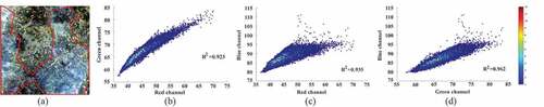
Correlation analysis was performed on four thin cloud images to confirm the above assumption. An example is shown in Figure 1, and the other three see Supplementary Figure S1. As the figures show, the scene is composed of various land covers, including vegetation, bare soil, and dark surface. The thin-cloud-contaminated regions, as indicated by the red polygons, are used to conduct the correlation analysis among the three visible bands, and the results are given subsequently. A strong correlation can be observed over cloudy regions between any two visible bands, with R² ranging between 0.923 and 0.962. Thus, the linear assumption in Equation (4)(4) $I_j=a_{i,j}\cdot I_i+b_{i,j}$(4) is robust for diverse land covers.

Figure 1. Correlation analysis among the visible bands of thin cloud image with different land covers: (a) observed thin cloud images, (b)–(d) band correlation analysis results of (a).

2.3.2. Derivation of the spectral transformation scheme

As mentioned previously, cloud contamination varies among the three visible bands. However, the transmission map estimated from the original thin cloud image using DCP is more suitable for the red band than the blue and green bands. This suitability is attributed to the following two aspects: First, electromagnetic radiation decreases with the increase in wavelength (Dave 1969; Gramotnev and Bozhevolnyi 2014), which means the red band with longer wavelength usually holds lower radiation than the blue and green bands with shorter wavelength; second, according to the scattering law, the red band is less vulnerable to thin cloud contamination than the blue and green bands (Chavez 1988; Zhang, Li, and Shen 2021). Therefore, in most visible remote sensing images, the red band typically has much lower radiation than the other two bands. As the DCP algorithm searches for pixels with minimum intensity among the three bands, most of the identified pixels are from the red band, and the transmission map estimated accordingly is thus more suitable for handling the red band.

Inspired by the above idea, we assume that if the dark pixels, which are identified by the DCP, mostly come from the blue or green bands, the estimated transmission maps can be more suitable for these two bands; therefore, the clouds in the two bands can be better corrected. Given the strong linear correlation among the three bands, we develop a spectral transformation scheme to derive different variant images for the accurate estimation of transmission maps in the blue and green bands.

For the green band, we make use of the linear relationship between the green and red bands to transform these two bands accordingly. Specifically, the green band is transformed to be a red-like band, and the red band is transformed to be a green-like band. The transformation is depicted as

(5) $\left\{\begin{array}{c}{I}_r^{T_1}=a_{g,r}\cdot I_g+b_{g,r}\\ I_g^{T_1}=a_{r,g}\cdot I_r+b_{r,g}\\ I_b^{T_1}=I_b\end{array}\right.$(5)

where $I$ denotes the original cloud-contaminated image, and $I_{\hspace{0.17em}}^{T_1}$ denotes the transformed image for estimating the green-band transmission. r, g, and b denote the red, green, and blue bands, respectively. $a_{g,r}$ and $b_{g,r}$ are the linear coefficients, which transform the green band into a red-like band, whereas $a_{r,g}$ and $b_{r,g}$ are the coefficients for transforming the red band into a green-like band. These linear coefficients can be estimated via Equation (4)(4) $I_j=a_{i,j}\cdot I_i+b_{i,j}$(4) by linearly regressing the cloud-covered pixels in the red and green bands. According to Equation (5)(5) $\left\{\begin{array}{c}{I}_r^{T_1}=a_{g,r}\cdot I_g+b_{g,r}\\ I_g^{T_1}=a_{r,g}\cdot I_r+b_{r,g}\\ I_b^{T_1}=I_b\end{array}\right.$(5) , the original green band is transformed into a red-like band with low intensity, and the DCP approach collects most dark object pixels from the red-like band, and thus, the transmission estimated from the transformed image $I_{\hspace{0.17em}}^{T_1}$ can be applied for cloud removal in the green band. Figure S2(a) in supplementary shows the transformed version $I_{\hspace{0.17em}}^{T_1}$ of the cloud-covered image in Figure 1(a).

Similarly, another transformed image $I_{\hspace{0.17em}}^{T_2}$ can be derived to accurately estimate the transmission map for the blue band, in which the blue band is transformed to be a red-like band and the red band is transformed to be a blue-like band. The transformation from the cloud-covered image $I$ to $I_{\hspace{0.17em}}^{T_2}$ is expressed as

(6) $\left\{\begin{array}{c}{I}_r^{T_2}=a_{b,r}\cdot I_b+b_{b,r}\\ I_g^{T_2}=I_g\\ I_b^{T_2}=a_{r,b}\cdot I_r+b_{r,b}\end{array}\right.$(6)

where $a_{b,r}$ and $b_{b,r}$ are the coefficients that transform the blue band into a red-like band, whereas $a_{r,b}$ and $b_{r,b}$ are the coefficients that transform the red band into a blue-like band. Figure S2(b) shows the transformed image $I_{\hspace{0.17em}}^{T_2}$ from the cloud-covered image in Figure 1(a). As shown in Equation (6)(6) $\left\{\begin{array}{c}{I}_r^{T_2}=a_{b,r}\cdot I_b+b_{b,r}\\ I_g^{T_2}=I_g\\ I_b^{T_2}=a_{r,b}\cdot I_r+b_{r,b}\end{array}\right.$(6) , most of the minimum-intensity pixels are from the transformed blue band, and thus, the estimated transmission can well characterize the thin cloud distribution in the blue band.

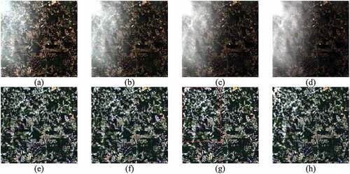
Three DCP maps are generated from the cloud-covered image $I$ and the transformed images $I_{\hspace{0.17em}}^{T_1}$ and $I_{\hspace{0.17em}}^{T_2}$, respectively. Figures 2a–c present the red (or red-like) bands of the three images, and Figures 2d–f show the DCP maps estimated from the three images accordingly. The DCP maps successfully characterize the variation of cloud radiation among different bands as they increase with the decrease in wavelength.

Figure 2. DCP maps estimated from the corresponding images $I_{\hspace{0.17em}}^{T_1}$and $I_{\hspace{0.17em}}^{T_2}$: (a)–(c) red (or red-like) bands of the original cloud-covered image and the two transformed images $I_{\hspace{0.17em}}^{T_1}$ and $I_{\hspace{0.17em}}^{T_2}$, (d)–(f) corresponding DCP maps estimated from the three images.

2.3.3. Estimation of spatially varied atmospheric light

Atmospheric light represents a portion of the radiation that does not come from the land surface during the imaging process (Narasimhan and Nayar 2002). In the traditional DCP approach devised for natural image dehazing, the atmospheric light is considered a global constant because natural photos are taken with narrow field angles in which the haze scattering intensity does not considerably change in space. However, remote sensing images are observed from space with wide swaths, and the cloud intensities in these scenes remarkably vary across different locations. A spatially varied atmospheric light map would therefore be more suitable for thin cloud correction in remotely sensed images.

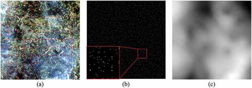
Given that dark objects can reflect scattering intensity in local patches, we develop a strategy to estimate atmospheric light locally, with the processing schematics illustrated in Figure 3. Specifically, a cloud-covered image is divided into several patches, as shown in Figure 3(a). Generally, the more even the thin clouds, the larger the patch size should be. Then, dark object pixels are identified in every patch to characterize atmospheric light locally and derive the result in Figure 3(b). The local dark pixels are interpolated to construct a continuous surface and produce the spatially varied atmospheric light map in Figure 3(c). High consistency can be observed between the estimated atmospheric light and the cloud distribution in the cloudy image, proving the validity of the presented strategy for atmospheric light estimation.

Figure 3. Procedure of the proposed scheme to estimate spatially varied atmospheric light: (a) patch division, (b) searching for dark object pixels in local patches, (c) estimated uneven atmospheric light.

2.3.4. Calculation of different transmissions for visible bands

After obtaining the DCP maps and the atmospheric light, we can estimate the transmission. For the red band, the transmission can be calculated on the basis of the DCP map from the original cloud covered image via the following equation:

(7) $t_r=1-\frac{I{}^{dark}}{A}$(7)

where $t_r$ is the red-band transmission, and $I^{dark}$ is the DCP map from the original cloud-covered image $I$. For the green and blue bands, the transmissions can be estimated on the basis of the inversely transformed DCP maps calculated from the images $I^{T_1}$ and $I^{T_2}$, which can be expressed as

(8) $t_g=1-\left(\frac{1}{A\cdot a_{g,r}}\cdot I^{T_1,dark}-\frac{b_{g,r}}{A\cdot a_{g,r}}\right)$(8)

(9) $t_b=1-\left(\frac{1}{A\cdot a_{b,r}}\cdot I^{T_2,dark}-\frac{b_{b,r}}{A\cdot a_{b,r}}\right)$(9)

where $t_g$ and $t_b$ are the green-band and blue-band transmission maps, respectively.

2.3.5. Correction procedure of thin clouds

As the transmission maps for three visible bands and the atmospheric light map are known, we can estimate the cloud-free image according to Equation (1)(1) $I\left(x\right)=J\left(x\right)t\left(x\right)+A\cdot \left(1-t\left(x\right)\right)$(1) , which can be formulated as follows:

(10) $\left\{\begin{array}{c}{J}_r=\frac{I_r-A}{t_r}+A\\ J_g=\frac{I_g-A}{t_g}+A\\ J_b=\frac{I_b-A}{t_b}+A\end{array}\right.$(10)

where $J_r$, $J_g$, and $J_b$ are surface radiation in the red, green, and blue bands, respectively. The three bands are composed to generate a clear image $J$.

3. Results and discussions

Remotely sensed images from Landsat 8 OLI, Landsat 7 ETM+, and GaoFen-2 were collected to perform thin cloud correction experiments. Simulated and real tests were conducted. To allow a comprehensive comparison, four baseline algorithms, namely, HOT (Zhang, Guindon, and Cihlar 2002), HTM (Makarau et al. 2014), traditional DCP (TDCP) (He, Sun, and Tang 2010), and SpA-GAN (Pan 2020), were used. The cloud correction performance was analyzed visually and quantitatively, that is, the visual comparison checks the spatial structure and spectral coherence of the recovered ground surfaces, whereas the quantitative assessment measures the consistency between recovered results and clear reference images by using three quantitative measures, including, root-mean-square error (RMSE), determination coefficient (R²), and spectral angle (SA).

3.1. Results based on simulated images

Simulated thin cloud images were generated in accordance with Equation (1)(1) $I\left(x\right)=J\left(x\right)t\left(x\right)+A\cdot \left(1-t\left(x\right)\right)$(1) , in which J is the cloud-free image acquired under clear-sky conditions, and A and t are estimated from real thin-cloud scenes. Cloud-free images were used as the ground truth to evaluate the results from visual and quantitative aspects. Three quantitative metrics were adopted to measure the radiometric consistency between corrected results and ground truth images, which can be formulated as (Willmott and Matsuura 2005; Dennison, Halligan, and Roberts 2004)

(11) $\mathrm{R}\mathrm{M}\mathrm{S}\mathrm{E}=\sqrt{1\text{overm}{\sum }_{i=1}^m{\left(J_i-{\hat{J}}_i\right)}^2}$(11)

(12) ${\mathrm{R}}^2=\frac{{\sum }_{i=1}^m{\left(J_i-\bar{J}\right)}^2}{{\sum }_{i=1}^m{\left({\hat{J}}_i-\bar{J}\right)}^2}$(12)

(13) $\mathrm{S}\mathrm{A}=\frac{1}{m}{\sum }_{i=1}^m{cos}^{-1}\frac{{\hat{J}}_i{J}_i^T}{\sqrt{J_i{J}_i^T}\sqrt{{\hat{J}}_i{\hat{J}}_i^T}}$(13)

where i is the spatial index of any pixel, m is the pixel number of the target image, J is the cloud-removed image from these approaches, $\bar{J}$ is the mean of the pixels in the cloud-removed image, and $\hat{J}$ is the ground-truth image.

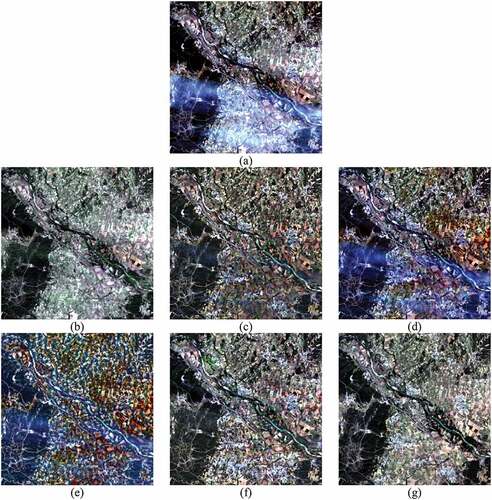
Two simulated tests were performed on the basis of Landsat 8 OLI and GaoFen-2 images, respectively. Figure 4 shows the simulated cloudy image, the recovered results, and the ground truth image in the Landsat-based simulated test. As shown in Figure 4(a), the scene is covered by large-area dark vegetation and some bright surfaces, and thin clouds are unevenly distributed in the upper part of the image. Figures 4b–f display the cloud-free results recovered by HOT, HTM, TDCP, SpA-GAN, and the proposed method, respectively, and Figure 4(g) shows the ground truth image used for assessing the performance of these methods. Specifically, HOT effectively removes thin clouds and recovers ground surface information, but its result suffers from spectral distortion, as revealed by the visual difference against the ground truth image. HTM removes the thinnest clouds and presents cloud-free results, which are highly consistent with the ground truth from spatial and spectral perspectives. However, HTM suffers from overcorrection over bright surfaces (i.e. bare soil) because it searches for dark objects on the basis of a single band, resulting in a limited number of dark pixels to be collected. TDCP performs well in maintaining spectral fidelity, but it cannot completely remove thin clouds because it ignores the spectral difference and the spatial variation of thin cloud intensity. SpA-GAN achieves satisfactory performance in thin cloud correction and ground information restoration. However, compared with the ground truth in Figure 4(g), a few thin clouds remain in the result. In contrast to the above methods, the proposed method successfully removes thin clouds and faithfully recovers ground surface information, presenting the cloud-free result, which is most consistent with the ground truth.

Figure 4. Comparison of the recovered results in the simulated experiment based on Landsat 8 OLI: (a) simulated cloud-covered image; (b)–(f) recovered results from HOT, HTM, TDCP, SpA-GAN, and the proposed method; (g) ground truth.

The quantitative results of the Landsat-based simulated test are given in Table 1, and the scores closest to the ideal ones are labeled bold. HTM has the lowest R² score and the highest RMSE score, indicating that its result is not well correlated with the ground truth in terms of radiometric fidelity. HOT holds the highest SA score, revealing that it has considerable spectral bias with the ground truth. SpA-GAN obtains better scores than the previous three methods in all metrics but slightly lower than that of the proposed method. The presented method obtains quantitative scores that are closest to the ideal ones, indicating that its result has the smallest radiometric deviation and highest spectral coherence to the reference image.

Table 1. Quantitative results of the four methods in the Landsat-based simulated data.

		HOT	HTM	TDCP	SpA-GAN	Proposed
Figure 4	R^2	0.6426	0.5583	0.8811	0.9421	0.9664
	RMSE	9.0707	11.9219	3.9321	2.2673	1.7380
	SA	3.2460	1.5115	1.5001	0.9916	0.7593

Figure 5 shows the results of the simulated test based on a GaoFen-2 image. In contrast to the above test, the scene in this test is interlaced with vegetation, bare soil, and rocks, and the thin clouds show considerable spatial variation. Generally, the visual findings are similar to those in the above test. HOT completely removes thin clouds, but its result shows spectral distortion in the whole scene. Even though thin clouds are diminished, some clouds remain in the result of HTM, and remarkable spectral distortions can be observed over bare soil regions. TDCP performs better to maintain spectral fidelity over noncloudy regions than HOT and HTM, but thin clouds cannot be totally removed in its result. SpA-GAN shows limited abilities in correcting the thin clouds for these data. In addition to the residual clouds, the color over the bare land considerably differs from the ground truth, suggesting poor spectral maintenance. In contrast, our approach not only well retains the spatial and spectral features over noncloudy regions but also completely corrects thin clouds in the scene, thus deriving the optimal cloud-free image. The quantitative results of this test are provided in Table 2. The proposed approach has the best scores in all three measures, obtaining the highest R² score of 0.9791, the lowest RMSE score of 0.9871, and the lowest SA score of 0.8870. The quantitative results indicate that the derived results from the proposed approach are well consistent with the ground-truth images.

Figure 5. Comparison of the recovered results in the simulated experiment based on GaoFen-2: (a) simulated cloud-covered image; (b)–(f) recovered results from HOT, HTM, TDCP, SpA-GAN, and the proposed method; (g) ground truth.

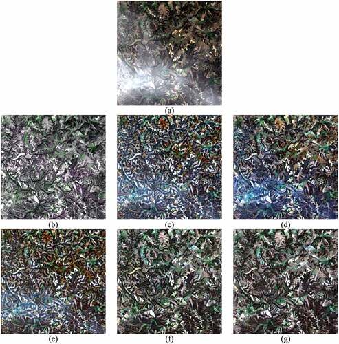
Table 2. Quantitative results of the four methods in the GaoFen-2-based simulated data.

		HOT	HTM	TDCP	SpA-GAN	Proposed
Figure 5	R^2	0.6411	0.6465	0.8360	0.8796	0.9791
	RMSE	10.6128	8.6219	3.3265	4.1671	0.9871
	SA	3.3608	1.3788	3.1053	2.4133	0.8870

3.2. Results based on real images

Six cloudy images were collected from Landsat 8 OLI, Landsat 7 ETM+, and GaoFen-2 to perform the real experiments, among which the first five images have 800 × 800 pixels and the last one has 8041 × 7041 pixels. The results of the first real experiment are presented in Figure 6. The Landsat 8 OLI image in Figure 6(a) is contaminated by uneven thin clouds, and it was acquired on 5 June 2018, with the central latitude and longitude of $320621\text{N},1140641\text{E}$. The primary land covers are vegetation and bare soil. Figures 6b–f show the cloud-removed images produced by HOT, HTM, TDCP, SpA-GAN, and the proposed approach. A detailed, band-by-band illustration of these color composite images is given in Figure S3 in Supplementary. HOT successfully removes the thin clouds and recovers the spatial structure information beneath the clouds, but the generated result in Figure 6(b) has a considerable spectral shift in comparison with spectral signals over noncloudy regions in the original input. HTM removes clouds from the scene and maintains ideal spectral features over noncloudy regions. However, the recovered results in regions originally covered by clouds are much darker than their noncloudy neighboring regions, indicating that HTM fails to recover the ground radiation faithfully. This limitation is primarily due to the fact that HTM cannot collect sufficient dark object pixels to estimate cloud intensity accurately because it searches only in an individual band for dark pixels. TDCP produces the result in Figure 6(d), from which we can see that it preserves noncloudy spectral signatures but fails to remove thin clouds completely. As previously mentioned, TDCP ignores the difference in thin cloud intensity among the three bands and applies a fixed transmission map for the three bands, resulting in the undercorrection of the cloud effects in shorter-wavelength bands, such as the blue band. Moreover, the globally constant atmospheric light in TDCP fails to consider the spatially uneven distribution of thin clouds. In Figure 6(e), the SpA-GAN successfully clears the adverse effects of thin clouds, and the spatial details are well enhanced in the result. In contrast, the spectra in the cloud-free regions are slightly shifted, suggesting limited spectral maintenance abilities. The cloud-free results produced by the proposed method are shown in Figure 6(f), and the three bands are shown in Figures S3(p)–(r) correspondingly. Our approach applies the spectral transformation scheme to derive transmission for each band individually, uses the local processing scheme to characterize the uneven distribution of cloud intensity, and thus produces the cloud-free image more convincing than other approaches. Visually, the result in Figure 6(f) recovers the ground spatial structures and maintains the spectral coherence between cloudy and noncloudy regions, thus confirming the remarkable capacities of our approach for thin cloud removal.

Figure 6. Comparison of recovered results in the first real data: (a) thin cloud image; (b)–(f) recovered results from HOT, HTM, TDCP, SpA-GAN, and the proposed method.

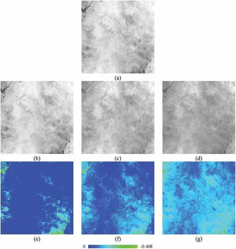
The proposed method and TDCP were designed on the basis of the DCP framework, and thus, both of them were compared to reveal the differences in the estimation of transmission. Figure 7(a) displays the transmission map in TDCP, in which a transmission map is constantly applied to the three bands, whereas Figure 7b–d show the three transmission maps separately used for the three bands in our approach. Figure 7e–g present the difference maps between Figure 7a-d, respectively. The transmission maps vary among the three bands and decrease from the red to blue bands, conforming to the scattering law. Thus, the spectral transformation scheme presented in this study can provide a more accurate and reasonable transmission map for each band than TDCP.

Figure 7. Transmission maps used in TDCP and the proposed method and their difference maps: (a) transmission map in TDCP, (b)–(d) transmission maps in the proposed method, (e)–(g) difference maps between (b)–(d) and (a).

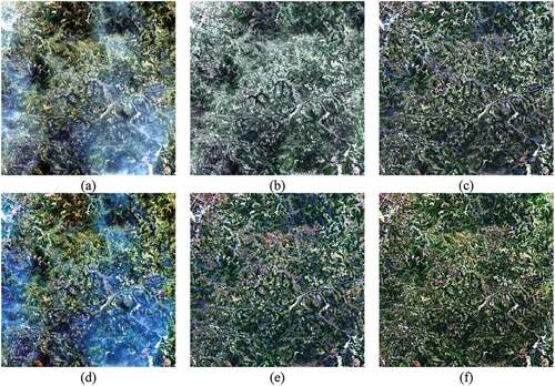
In the second real experiment, the remotely sensed image captured by GaoFen-2 shown in Figure 8(a) was used, in which thin clouds occupied the northwest part of the image. The central latitude and longitude of the image are $30445\text{N},10935\text{E}$. Figures 8b-f display the results derived from HOT, HTM, TDCP, SpA-GAN, and our approach, respectively. HOT completely removes the thin cloud but fails to preserve spectral fidelity and spatial structures in the cloudy regions. HTM produces cloud-removed results, yet it suffers from serious spectral distortions because the cloudy region is visually darker than the noncloudy region after cloud removal. Despite its good ability to maintain spectral fidelity, TDCP is limited in removing clouds completely. SpA-GAN keeps well the color in cloud-free regions. In addition, most of the thin clouds are eliminated, and only a few remain. In contrast, the proposed approach not only corrects thin clouds but also recovers the land surface information in spatial and spectral dimensions, thus demonstrating a better performance to derive ideal outputs.

Figure 8. Comparison of recovered results in the second real data: (a) thin cloud image; (b)–(f) recovered results from HOT, HTM, TDCP, SpA-GAN, and the proposed method.

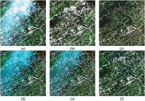
The results of the third and fourth real experiments are shown in Figures S4 and S5. The thin cloud image in Figure S4(a) is captured by Landsat 8 OLI on 1 July 2014, which is centered at $44546\text{N},4122\text{E}$. Figure S5(a) is acquired by GaoFen-2 at $45052\text{N},4456\text{E}$. The thin clouds in these two scenes are distributed unevenly in space, and more importantly, the cloudy and cloud-free regions present clear boundaries, which is challenging for accurate cloud correction. As shown in Figures S4 and S5, the four benchmark approaches suffer from incomplete cloud correction and considerable spectral distortion. In contrast, the proposed method successfully suppresses thin clouds and recovers ground surface information.

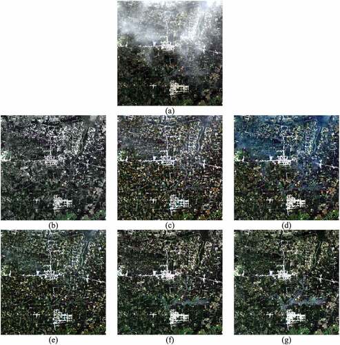
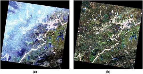
The cloudy image and the cloud-removed results in the fifth experiment are displayed in Figure 9. The cloudy image in Figure 9(a) was captured by Landsat 8 OLI on September 21^st, 2016, centered at $44026\text{N},4026\text{E}$. It is covered with vegetation, bare soil, forest, and some artificial buildings and is contaminated by thin clouds in the southern part. Figures 9b-f show the results derived from HOT, HTM, TDCP, SpA-GAN, and our method. In addition, the observed image in Figure 9(g) was collected from the same place with a temporal gap of 16 days and was used as reference for comparison. The visual assessment has similar findings as in the previous tests, that is, HOT and HTM cannot recover proper spectral signatures, whereas TDCP and SpA-GAN, despite maintaining spectral features to a certain degree, show limited ability to remove clouds completely. In contrast, the proposed approach not only removes clouds successfully but also recovers the land surface radiation faithfully. The produced result in Figure 9(f) is visually closest to the evaluation reference in Figure 9(g), as compared with the other results.

Figure 9. Comparison of recovered results in the fifth real data: (a) thin cloud image; (b)–(f) recovered results from HOT, HTM, TDCP, SpA-GAN, and the proposed method; (g) cloud-free image acquired temporally adjacent to (a).

Given that a temporally adjacent cloud-free image is collected as an evaluation reference, quantitative assessment can be performed in the test. Table 3 reports quantitative assessment results in terms of RMSE, R², and SA, and the scores closest to the ideal ones are labeled bold. Generally, HOT obtains the highest RMSE and SA scores and the lowest R² scores, indicating that it has the most considerable radiation deviation from the reference image. HTM, TDCP, and SpA-GAN obtain scores closer to ideal ones than HOT. As the best-performed approach, the proposed approach has the best performance in each of the three measures, with the lowest RMSE scores ranging from 2.0189 to 2.4711 and the highest R² scores ranging from 0.8906 to 0.9469. The quantitative results confirm the same finding in the previous analysis that our approach can remove thin clouds completely and retrieve land surface radiation accurately.

Table 3. Quantitative results of the four approaches in the fifth real data.

			RMSE	R^2	SA
Figure 9	HOT	Red	7.4211	0.6143	1.2143
		Green	8.9114	0.8162
		Blue	8.8453	0.7651
	HTM	Red	5.0133	0.7641	0.7622
		Green	5.5411	0.8321
		Blue	6.3654	0.8896
	TDCP	Red	4.5614	0.8825	0.8146
		Green	6.6631	0.8151
		Blue	7.1002	0.8162
		Red	4.9121	0.8246
	SpA-GAN	Green	6.1746	0.8119	0.8011
		Blue	6.2449	0.8473
	Proposed	Red	2.4711	0.8906	0.3912
		Green	2.1649	0.9147
		Blue	2.0189	0.9469

To test the thin cloud correction performance of the proposed method for large-sized images, we collected a full-scene Landsat 7 ETM+ image for the last real experiment. The scene in Figure 10(a) centers at $31657\text{N},112447\text{E}$was observed over Wuhan, China, on 9 July 2002. The land covers are complex, including waterbodies, vegetation, built-up areas, and bare soil. The thin clouds are spatially varied and contaminated almost half part of the scene. The results of our approach are shown in Figure 10(b), in which all thin clouds are totally removed. Moreover, the comparison of noncloudy regions between Figures 10a and b reveals that the proposed method demonstrates good capacities to maintain spectral fidelity. In summary, our approach can yield satisfactory cloud-removed results for remote sensing images from different sensors with diverse land covers and spatial sizes.

Figure 10. Comparison of recovered results in the sixth real data: (a) full-scene thin cloud-covered image, (b) recovered result from the proposed method.

4. Discussion

The effectiveness of the proposed method on thin cloud correction was verified by the above simulated and real experiments. However, some problems of limitations and applicability must be discussed and analyzed.

4.1. Factors affecting thin cloud correction performance

First, how cloud cover rates and cloud thickness affect the performance of the method should be discussed. To clarify this problem, a series of simulated thin cloud images were generated using different transmission maps, as shown in Figures 11–13.

Figure 11. Real visible image captured by Landsat 8 OLI (path/row: 019/037) on May 12, 2022.

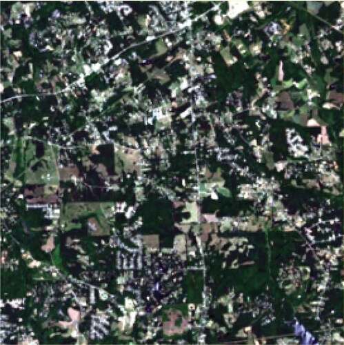
Figure 12. Four simulated thin cloud images with different cloud cover rates. The first row is the simulated thin cloud images, the second row is the ground truths of transmission maps, and the third row shows the corrected results using the proposed method.

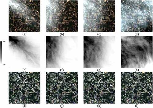
Figure 13. Four simulated thin cloud images with different cloud thicknesses. The first row is the simulated thin cloud images, and the second row shows the corrected results using the proposed method.

In Figure 11, a real visible image acquired by Landsat 8 OLI is selected as the ground truth, based on which four simulated thin cloud images with different cloud cover rates are produced, as exhibited in the first row of Figure 12. The ground truths of various transmission maps are given in the second row, in which the values of these transmission maps vary from 0.6 to 1.0. The cloud cover rates of Figures 12e–h are nearly close to 40%, 60%, 80%, and 100%. The corrected results are given in the last row. As shown by the results, all the thin clouds are totally corrected, and the degraded ground features are recovered faithfully. This result can be attributed to the fact that the transmission values vary from 0.6 to 1.0, suggesting that the ground information accounts for at least 60% of the information of cloudy areas. Therefore, dark objects can still be identified, and the transmission maps can be precisely estimated. Thus, cloud cover rates in a scene do not considerably influence the cloud correction performance of the proposed method.

To investigate further the effects of cloud thickness on the method performance, Figure 11 was used again as ground truth to yield the simulated thin cloud images shown in the first row of Figure 13. The transmission map values used in Figures 13a-d vary between 0.6 and 1.0, 0.4 and 0.8, 0.2 and 0.6, and 0 and 0.4, respectively. The corrected results using the proposed method are shown in the last rows. Clearly, the thin clouds in Figures 13a and b can be completely removed, whereas clouds in Figure 13(c) are partly removed, and a small amount remains, as indicated by the red rectangle in Figure 13(g). Similarly, the cloud residue can be seen in the fourth result. The reasons for this can be explained as follows: In Figures 13c and d, the transmission values vary between 0.2 and 0.6 and 0 and 0.4. Too small transmissions, such as 0.2 or even 0, indicate little or even no ground information in cloudy areas, which are approaching thick clouds. Thus, the collected dark objects may be inaccurate and unreliable, resulting in incorrect transmission maps and residue clouds.

Therefore, cloud cover rates in a scene have minimal influence on the cloud correction performance of the proposed method, whereas cloud thickness may limit the feasibility of the proposed method. When the cloud thickness is close to the thick clouds, strategies for correcting thick clouds, such as pixel replacement, should be considered.

In addition, the proposed method may not be fully applicable in some cases. As our approach is devised on the basis of the DCP framework, it is dependent on the basic assumption that sufficient dark objects exist in the scene. Thus, forscenes dominated by bright surfaces, such as snow and bare soil, the DCP-based methods cannot estimate transmission intensity accurately, resulting in an overcorrection problem. This issue of how to deal with scenes dominated by bright surfaces will be explored in our future studies.

4.2. Applicability to other sensors

The applicability of the proposed method to other sensors with visible bands is another issue that must be investigated. Two different real visible images were collected from two open-source datasets, i.e. WHUS2-CR (Li et al. 2020) and RICE (Lin et al. 2019), to conduct the experiments, as shown in Figures S6 and S7 in Supplementary.

The first to third columns in Figures S6 and S7 are the thin cloud images, the corrected results, and the referenced ground truth, respectively. The thin clouds can be completely removed by the proposed method. Furthermore, the recovered spatial and spectral details are consistent with the referenced ground truth. The findings indicate that the proposed method is effective for other sensors with visible bands, and the recovered ground features are accurate and acceptable.

5. Conclusion

Thin cloud contamination is a common and ineluctable issue in optical remote sensing images. In this study, we proposed an approach for thin cloud correction. The highlights can be summarized from two aspects. First, on the basis of the strong linear correlation among the three visible bands, a spectral transformation scheme was developed to derive transformed images, based on which band-specific transmission maps can be estimated for three visible bands. Second, given the uneven distribution of cloud covers in remote sensing images, a patch-based scheme is presented to estimate atmospheric light locally and generate spatially varied atmospheric light maps. The spectrally varied transmission maps and the spatially varied atmospheric light maps yielded more natural cloud-free results. Simulationand real experiments based on Landsat 8 OLI, Landsat 7 ETM+, and GaoFen-2 images were conducted to validate the advantages of the proposed method over the other four baselines. Visually, our approach can remove thin clouds completely and reproduce spectral signatures of ground objects faithfully. Quantitatively, the proposed method achieves better scores than the baseline methods. In simulation and real experiments, the proposed method obtains R² values (>0.8906) and low root-mean-square errors (<2.4711) and spectral angle maps (<0.8870), which are superior to the baseline approaches. In addition, the factors affecting the thin cloud correction performance and the applicability to other sensors were investigated. In summary, the proposed method is effective for correcting thin clouds in visible images acquired by different satellites, and the recovered spatial and spectral structure information are accurate and acceptable.

Acknowledgments

We acknowledge the USGS and CRESDA teams for the free access to Landsat 7 ETM+, Landsat 8 OLI, and GaoFen-2 images.

Disclosure statement

The authors declare that they have no known competing financial interests or personal relationships that could have appeared to influence the work reported in this paper.

Data availability statement

Landsat 7 ETM+ and Landsat 8 OLI images are available from USGS (https://earthexplorer.usgs.gov/). GaoFen-2 images are available and can be accessed from http://www.cresda.com/CN/.

Additional information

Funding

This work was supported by Guangdong Enterprise Key Laboratory for Urban Sensing, Monitoring and Early Warning (No.2020B121202019), China Postdoctoral Science Foundation (No.2022M713551), and Guangdong Basic and Applied Basic Research Foundation (No. 2022A1515110095)

References

- Chanda, B., and D. Majumder. 1991. “An Iterative Algorithm for Removing the Effect of Thin Cloud Cover from LANDSAT Imagery.” Mathematical Geology 23 (6): 853–18. doi:10.1007/BF02068780.
- Chavez, P. S., Jr. 1988. “An Improved Dark-Object Subtraction Technique for Atmospheric Scattering Correction of Multispectral Data.” Remote Sensing of Environment 24 (3): 459–479. doi:10.1016/0034-4257(88)90019-3.
- Chen, S., X. Chen, J. Chen, P. Jia, X. Cao, and C. Liu. 2015. “An Iterative Haze Optimized Transformation for Automatic Cloud/Haze Detection of Landsat Imagery.” IEEE Transactions on Geoscience Remote Sensing 54 (5): 2682–2694. doi:10.1109/TGRS.2015.2504369.
- Dave, J. V. 1969. “Scattering of Electromagnetic Radiation by a Large, Absorbing Sphere.” IBM Journal of Research Development 13 (3): 302–313. doi:10.1147/rd.133.0302.
- Delac, K., M. Grgic, and T. Kos. 2006. Sub-Image Homomorphic Filtering Technique for Improving Facial Identification Under Difficult Illumination Conditions. Paper presented at the International Conference on Systems, Signals and Image Processing, September 21-23, Budapest, Hungary.
- Dennison, P. E., K. Q. Halligan, and D. A. Roberts. 2004. “A Comparison of Error Metrics and Constraints for Multiple Endmember Spectral Mixture Analysis and Spectral Angle Mapper.” Remote Sensing of Environment 93 (3): 359–367. doi:10.1016/j.rse.2004.07.013.
- Dharejo, F. A., Y. Zhou, F. Deeba, M. A. Jatoi, Y. Du, and X. Wang. 2021. “A Remote‐sensing Image Enhancement Algorithm Based on Patch‐wise Dark Channel Prior and Histogram Equalisation with Colour Correction.” IET Image Processing 15 (1): 47–56. doi:10.1049/ipr2.12004.
- Duan, C., J. Pan, and R. Li. 2020. “Thick Cloud Removal of Remote Sensing Images Using Temporal Smoothness and Sparsity Regularized Tensor Optimization.” Remote Sensing 12 (20): 3446. doi:10.3390/rs12203446.
- Du, Y., B. Guindon, and J. Cihlar. 2002. “Haze Detection and Removal in High Resolution Satellite Image with Wavelet Analysis.” IEEE Transactions on Geoscience Remote Sensing 40 (1): 210–217. doi:10.1109/36.981363.
- Fritz, S., L. See, C. Perger, C. S. McCallum, M. Schepaschenko, D. Duerauer, C. Karner, et al. 2017. “A Global Dataset of Crowdsourced Land Cover and Land Use Reference Data.” Scientific Data 4 (1): 170075. doi:10.1038/sdata.2017.75.
- Gao, B., and R. Li. 2017. “Removal of Thin Cirrus Scattering Effects in Landsat 8 OLI Images Using the Cirrus Detecting Channel.” Remote Sensing 9 (8): 834. doi:10.3390/rs9080834.
- Gramotnev, D. K., and S. I. Bozhevolnyi. 2014. “Nanofocusing of Electromagnetic Radiation.” Nature Photonics 8 (1): 13–22. doi:10.1038/nphoton.2013.232.
- He, K., J. Sun, and X. Tang. 2010. “Single Image Haze Removal Using Dark Channel Prior.” IEEE Transactions on Pattern Analysis Machine Intelligence 33 (12): 2341–2353. doi:10.1109/TPAMI.2010.168.
- Jia, K., B. Cai, C. Qing, X. Xu, and D. Tao. 2016. “Dehaze Net: An End-To-End System for Single Image Haze Removal.” IEEE Transactions on Image Processing 25 (11): 5187–5198. doi:10.1109/TIP.2016.2598681.
- Kauth, R. J., and G. Thomas. 1976. “The Tasselled Cap–A Graphic Description of the Spectral-Temporal Development of Agricultural Crops as Seen by Landsat.” LARS Symposia 1976: 159.
- Lee, S., S. Yun, J. Nam, C. Won, and S. Jung. 2016. “A Review on Dark Channel Prior Based Image Dehazing Algorithms.” EURASIP Journal on Image Video Processing 2016 (1): 1–23. doi:10.1186/s13640-016-0104-y.
- Liang, S., H. Fang, and M. Chen. 2001. “Atmospheric Correction of Landsat ETM+ Land Surface Imagery. I Methods.” IEEE Transactions on Geoscience and Remote Sensing 39 (11): 2490–2498.
- Li, J., Q. Hu, and M. Ai. 2018. “Haze and Thin Cloud Removal via Sphere Model Improved Dark Channel Prior.” IEEE Geoscience Remote Sensing Letters 16 (3): 472–476. doi:10.1109/LGRS.2018.2874084.
- Li, W., Y. Li, D. Chen, and J. C. Chan. 2019. “Thin Cloud Removal with Residual Symmetrical Concatenation Network.” ISPRS Journal of Photogrammetry Remote Sensing 153: 137–150. doi:10.1016/j.isprsjprs.2019.05.003.
- Lin, D., G. Xu, X. Wang, Y. Wang, X. Sun, and K. Fu. (2019). “A Remote Sensing Image Dataset for Cloud Removal.” arXiv preprint arXiv:1901.00600.
- Liu, J., X. Wang, M. Chen, S. Liu, X. Zhou, Z. Shao, and P. Liu. 2014. “Thin Cloud Removal from Single Satellite Images.” Optics Express 22 (1): 618–632. doi:10.1364/OE.22.000618.
- Li, J., Z. Wu, Z. Hu, J. Zhang, M. Li, L. Mo, and M. Molinier. 2020. “Thin Cloud Removal in Optical Remote Sensing Images Based on Generative Adversarial Networks and Physical Model of Cloud Distortion.” ISPRS Journal of Photogrammetry Remote Sensing 166: 373–389. doi:10.1016/j.isprsjprs.2020.06.021.
- Li, H., L. Zhang, H. Shen, and P. Li. 2012. “A Variational Gradient-Based Fusion Method for Visible and SWIR Imagery.” Photogrammetric Engineering Remote Sensing 78 (9): 947–958. doi:10.14358/PERS.78.9.947.
- Lv, H., Y. Wang, and Y. Gao. 2018. Using Independent Component Analysis and Estimated Thin-Cloud Reflectance to Remove Cloud Effect on Landsat-8 Oli Band Data. 2018 IEEE International Geoscience and Remote Sensing Symposium, Valencia, Spain, 18261166.
- Lv, H., Y. Wang, and Y. Shen. 2016. “An Empirical and Radiative Transfer Model Based Algorithm to Remove Thin Clouds in Visible Bands.” Remote Sensing of Environment 179: 183–195. doi:10.1016/j.rse.2016.03.034.
- Lv, H., Y. Wang, and Y. Yang. 2018. “Modeling of Thin-Cloud TOA Reflectance Using Empirical Relationships and Two Landsat-8 Visible Band Data.” IEEE Transactions on Geoscience Remote Sensing 57 (2): 839–850. doi:10.1109/TGRS.2018.2861939.
- Makarau, A., R. Richter, R. Müller, and P. Reinartz. 2014. “Haze Detection and Removal in Remotely Sensed Multispectral Imagery.” IEEE Transactions on Geoscience Remote Sensing 52 (9): 5895–5905. doi:10.1109/TGRS.2013.2293662.
- Narasimhan, S. G., and S. K. Nayar. 2002. “Vision and the Atmosphere.” International Journal of Computer Vision 48 (3): 233–254. doi:10.1023/A:1016328200723.
- Pan, H. 2020. “Cloud Removal for Remote Sensing Imagery via Spatial Attention Generative Adversarial Network.” arXiv preprint arXiv:2009.13015.
- Pang, Y. Y. Z., Y. Wang, X. Wei, and B. Chen. 2022. “SOCNet: A Lightweight and Fine-Grained Object Recognition Network for Satellite-On-Orbit Computing.” IEEE Transactions on Geoscience and Remote Sensing 60: 1–13. doi:10.1109/TGRS.2022.3216215.
- Poggio, L., A. Gimona, and I. Brown. 2012. “Spatio-Temporal MODIS EVI Gap Filling Under Cloud Cover: An Example in Scotland.” ISPRS Journal of Photogrammetry Remote Sensing 72: 56–72. doi:10.1016/j.isprsjprs.2012.06.003.
- Shen, H., H. Li, Y. Qian, L. Zhang, and Q. Yuan. 2014. “An Effective Thin Cloud Removal Procedure for Visible Remote Sensing Images.” ISPRS Journal of Photogrammetry Remote Sensing 96: 224–235. doi:10.1016/j.isprsjprs.2014.06.011.
- Shen, X., Q. Li, Y. Tian, and L. Shen. 2015. “An Uneven Illumination Correction Algorithm for Optical Remote Sensing Images Covered with Thin Clouds.” Remote Sensing 7 (9): 11848–11862. doi:10.3390/rs70911848.
- Sumbul, G., R. G. Cinbis, and S. Aksoy. 2017. “Fine-Grained Object Recognition and Zero-Shot Learning in Remote Sensing Imagery.” IEEE Transactions on Geoscience Remote Sensing 56 (2): 770–779. doi:10.1109/TGRS.2017.2754648.
- Wen, X., Z. Pan, Y. Hu, and J. Liu. 2022. “An Effective Network Integrating Residual Learning and Channel Attention Mechanism for Thin Cloud Removal.” IEEE Geoscience Remote Sensing Letters 19: 1–5. doi:10.1109/LGRS.2022.3161062.
- Willmott, C. J., and K. Matsuura. 2005. “Advantages of the Mean Absolute Error (MAE) Over the Root Mean Square Error (RMSE) in Assessing Average Model Performance.” Climate Research 30 (1): 79–82. doi:10.3354/cr030079.
- Wu, J., X. Wang, B. Zhong, A. Yang, K. Jue, J. Wu, L. Zhang, W. Xu, S. Wu, and N. Zhang. 2020. “Ecological Environment Assessment for Greater Mekong Subregion Based on Pressure-State-Response Framework by Remote Sensing.” Ecological Indicators 117: 106521. doi:10.1016/j.ecolind.2020.106521.
- Xu, M., F. Deng, S. Jia, X. Jia, and A. J. Plaza. 2022. “Attention Mechanism-Based Generative Adversarial Networks for Cloud Removal in Landsat Images.” Remote Sensing of Environment 271: 112902. doi:10.1016/j.rse.2022.112902.
- Xu, M., X. Jia, M. Pickering, and S. Jia. 2019. “Thin Cloud Removal from Optical Remote Sensing Images Using the Noise-Adjusted Principal Components Transform.” ISPRS Journal of Photogrammetry Remote Sensing 149: 215–225. doi:10.1016/j.isprsjprs.2019.01.025.
- Zhang, Y., B. Guindon, and J. Cihlar. 2002. “An Image Transform to Characterize and Compensate for Spatial Variations in Thin Cloud Contamination of Landsat Images.” Remote Sensing of Environment 82 (2–3): 173–187. doi:10.1016/S0034-4257(02)00034-2.
- Zhang, C., H. Li, and H. Shen. 2021. “A Scattering Law Based Cirrus Correction Method for Landsat 8 OLI Visible and Near-Infrared Images.” Remote Sensing of Environment 253: 112202. doi:10.1016/j.rse.2020.112202.
- Zhang, C. C. L., B. Li, F. Zhao, and C. Zhao. 2022. “Spatiotemporal Neural Network for Estimating Surface NO2 Concentrations Over North China and Their Human Health Impact.” Environmental Pollution 162: 119510. doi:10.1016/j.envpol.2022.119510.
- Zhang, Q., Q. Yuan, J. Li, Z. Li, and H. Shen. 2020. “Thick Cloud and Cloud Shadow Removal in Multitemporal Imagery Using Progressively Spatio-Temporal Patch Group Deep Learning.” Isprs Journal of Photogrammetry and Remote Sensing 162: 148–160. doi:10.1016/j.isprsjprs.2020.02.008.