National-scale mapping of building footprints using feature super-resolution semantic segmentation of Sentinel-2 images

ABSTRACT

Since buildings are closely related to human activities, large-scale mapping of individual buildings has become a hot research topic. High-resolution images with sub-meter or meter resolution are common choices to produce maps of building footprints. However, high-resolution images are both infrequently collected and expensive to obtain and process, making it very difficult to produce large-scale maps of individual buildings timely. This paper presents a simple but effective way to produce a national-scale map of building footprints using feature super-resolution semantic segmentation of sentinel-2 images. Specifically, we proposed a super-resolution semantic segmentation network named EDSR_NASUnet, which is an end-to-end network to generate semantic maps with a spatial resolution of 2.5 m from real remote sensing images with a spatial resolution of 10 m. Based on the dataset consisting of images from 35 cities in China, we quantitatively compared the proposed method with three methods under the same framework and qualitatively evaluated the identification results of individual buildings. In addition, we mapped building footprints within the entire China at 2.5 m-resolution using Sentinel-2 images of 10 m resolution. The density of building footprints varies considerably across China, with a gradual increase in building footprints from west to east, i.e. from the first step of China’s terrain to the third one. We detected over 86.3 million individual buildings with a total rooftop area of approximately 58,719.43 km². The number of buildings increased from 5.73 million in the first step of China’s terrain, through 23.41 million in the second step of China’s terrain, to 57.16 million in the third step of China’s terrain. The area of buildings also increased from 3318.02 km² through 13,844.29 to 41,557.12 km². The Aihui-Tengchong line, a dividing line representing the regional distribution of China’s population, also divides the regional distribution of Chinese buildings. Our approach has a more open and practical application because of the medium-resolution images and platform with open access. Results are available to the community (https://code.earthengine.google.com/?asset=users/flower/2019_China).

KEYWORDS:

• Building footprints
• super-resolution semantic segmentation
• single building
• national-scale
• Sentinel-2

1 Introduction

The building is one of the most important features that characterize human activities. Due to population growth and urbanization, the distribution of buildings is rapidly changing (Frolking et al. 2013). Timely and reliable access to building spatial distribution information is of great significance in the study of global environmental change, the rapid update of urban spatial information, disaster monitoring and mitigation, and so on. However, although the traditional manual digitizing method has high accuracy, it cannot meet the demand for fast extraction and updating of building information in large area and complex scenes due to high workload and low efficiency. With the development of remote sensing technology, large-scale mapping of built-up areas or individual buildings has gradually become a hot topic in recent years.

As shown in Table 1, although substantial progress has been made since the first product was reported in the early 1990s, mapping individual buildings at national- or global-scale remains a complex challenge. Most of the work done on low- (i.e. 100–1000 m) and medium-resolution (i.e. 10–100 m) in previous studies extracted the built-up areas from remote sensing images. These built-up areas consist mainly of impervious surfaces with buildings, roads, squares, etc. High-resolution images with submeter are often utilized to map individual buildings in recent years. However, due to the high cost of image acquisition and the poor coverage of high-resolution images from single-satellite source, the geographical coverage of maps of individual buildings might be very limited or it is very difficult to update in a regular time interval. The selection of multi-spectral satellite images like Sentinel-2 with a spatial resolution up to 10 m, which are open access, is an alternative option to solve the above dilemma. This work mainly focuses on solving the challenge of extracting the individual building footprints from the 10-m spatial resolution Sentinel-2 images using the proposed deep learning model.

Table 1. Large-scale products of building areas or buildings with different spatial resolution.

Resolution	Abbreviation (Citation)	Producer	Image	Resolution	Definition of building	Methods
low- resolution (100-1000m)	IGBP DISCover (Loveland and Belward 1997)	United States Geological Survey	AVHRR 1 km data	1 km	Urban and build-up	Unsupervised clustering
	UMD Land Cover Classification (Hansen et al. 2000)	University of Maryland	AVHRR 1 km data	1 km	Urban and build-up	Supervised classification tree
	DMSP-OLS Nighttime Lights (Elvidge et al. 2001)	US National Geophysical Data Center	DMSP-OLS 2.2 km data	927 m	Nighttime illumination intensity	Data compositing
	MCD12Q1 (Friedl et al. 2002)	United States Geological Survey	MODIS Terra and Aqua data	500 m–1 km	Urban and build-up lands	Supervised classification
	GLC2000 (Bartholomé and Belward 2005)	European Commission Joint Research Center	SPOT-Vegetation, Nighttime lights data	988 m	Artificial surfaces and associated areas	Unsupervised classification
	GRUMP (Balk et al. 2006)	Earth Institute at Columbia University	Urban extent	927 m	VMAP, census data, Nighttime lights, maps	Data fusion by logarithmic regression
	IMPSA (Elvidge et al. 2007)	US National Geophysical Data Center	Landscan, Nighttime lights data	927 m	Density of impervious surface area	Data fusion by linear regression
	GLCNMO (Tateishi et al. 2011)	Global Land Cover by National Mapping Organization	MODIS Terra and Aqua data	500 m–1 km	Urban	Supervised classification
	GLOBCOVER (Bicheron et al. 2011)	European Space Agency	MERIS	309 m	Artificial surfaces and associated areas	Unsupervised classification
medium- resolution (10-100m)	NLCD 2001 (Homer et al. 2004)	Multi-Resolution Land Characteristics	Landsat 5/7 images	30 m	Developed, open space、Developed, low/medium/high intensity	Decision tree
	FROM_GLC30 (Gong et al. 2013)	Tsinghua University	Landsat TM and ETM+ data	30 m	Impervious surface	supervised classifiers，including MLC, the J4.8 decision tree classifier, the RF and SVM.
	GlobalLand30 (Chen et al. 2015)	Tongji University	Landsat TM5、ETM+、OLI data and HJ-1 data	30 m	Artificial surface	A Pixel-Object-Knowledge-based (POK-based) classification
	GUF (Esch et al. 2013)	German Aerospace Center	TerraSAR-X and TanDEM-X	12 m	Urban building footprint	Urban footprint processor
	FROM_GLC10 (Gong et al. 2019)	Tsinghua University	Sentinel-2 imagery	10 m	Impervious surface	Random forest classifier
	WSF 2015/2019 (Marconcini et al. 2021, 2020)	Earth Observation Center	Landsat-8 and Sentinel-1 imagery	10 m	Human settlements	Support Vector Machines (SVMs)
	ESA_WorldCover (Zanaga et al. 2021)	European Space Agency	Sentinel-1 and Sentinel-2 imagery	10 m	Built-up	Gradient boosting decision tree algorithm
	GHS-BUILT-S (Corbane et al. 2021)	European Commission, Joint Research Center	Sentinel-2 composite and Landsat data	10 m	Built-up surface	Symbolic machine learning
	Esri_Land_Cover_2020 (Karra et al. 2021)	Esri	Sentinel-2 imagery	10 m	Built Area	Deep learning
	Dynamic World dataset (Brown et al. 2022)	Google and the World Resources Institute	Sentinel-2 imagery	10 m	Built Area	Deep learning
high-resolution (<10 m)	Open Street Map (Heipke 2010)	OpenStreetMap Foundation	Mobile tracing and satellite imagery	Submeter	Buildings	Mobile tracing and satellite imagery interpretation
	Bing Maps (Yang et al. 2018)	Microsoft	High-resolution satellite images	Submeter	Buildings	Deep learning
	Google Earth (Sirko et al. 2021)	Google	High-resolution satellite images	Submeter	Buildings	Deep learning
	Tiandi Map	Ministry of Natural Resources, People’s Republic of China	High-resolution satellite images	Submeter	Buildings	Deep learning

The major contributions of this paper are summarized as follows: (1) A new neural network, i.e. the EDSR_NASUnet, has been proposed, which is shown to be an effective way to extract high-resolution building footprints from medium-resolution Sentinel-2 images; (2) The building footprint product of China in 2019 with 2.5 m resolution from Sentinel-2 images has been produced; and (3) The feasibility of extracting individual building footprints from Sentinel-2 images has been discussed in detail.

The remainder of this paper is organized as follows. Related works are reviewed in Section 2. The study area is described in Section 3. The data source and preprocessing are described in Section 4. The proposed method is described in Section 5, where details of the algorithms, as well as the evaluation metrics, are also presented. The experimental results and the map of buildings in China are given in Section 6. The feasibility of extracting building footprints from Sentinel-2 images and the performance of the proposed method are discussed in Section 7. Finally, the conclusions are drawn in Section 8.

2 Related works

Recently, identification of individual buildings has started to emerge with the availability of high spatial resolution satellite images at meter- or submeter resolution, such as WorldView, QuickBird, and GaoFen series (Rimal et al. 2020; Luo et al. 2019; Huang et al. 2017; Chen et al. 2002). Meanwhile, some deep learning algorithms, such as convolutional neural network (CNN) and deep neural network (DNN), have greatly improved the performance of semantic segmentation (SS) (Jiayi et al. 2022; Guangming et al. 2018; Maggiori et al. 2017; Yuan 2018). As a research hotspot in remote sensing image processing, U-Net has achieved good performance in building footprints mapping (Kriti, Bodani, and Sharma 2022; Ayala, Aranda, and Galar 2021). An enhanced hourglass-shaped network was proposed based on the U-Net, and simultaneously improved accuracy and reduced the network volume in extraction of building footprints (Liu et al. 2017). The combination of U-Net and ResNet enabled to obtain higher accuracy on building footprints extraction with the use of artificially extracted features as input (Yongyang et al. 2018). U-NASNetMobille (Yang and Tang 2020), proposed on the basis of NASNet-Mobile (Zoph et al. 2018), was used for building footprint extraction in 100 cities in different continents, and achieved good generalization performance. However, it is rather difficult to obtain large-scale and high-resolution remote sensing images in a specific time interval. Iterative self-organizing SCEne-Level sampling (ISOSCELES) was proposed to solve the challenge of obtaining complex and multimodal sample sets in remote sensing images for large-scale building extraction (Benjamin et al. 2022). Most of the building footprint products based on high-resolution satellite images are limited to the urban scale (Jiayi et al. 2022; Zhang et al. 2021). While large-scale high-resolution building mapping products have currently achieved by some commercial companies with mass storage infrastructures, high-performance computing platforms and amounts of high-resolution imagery, like Microsoft (Yang 2018), Meta, and Google (Sirko et al. 2021), and crowdsourcing data, e.g. Open Street Map (OSM) (Heipke 2010), these high-resolution data typically have the following characteristics: multi-sources, multi-temporal, and multi-scale (Khoshboresh-Masouleh and Shah-Hosseini 2021; Hasan, Shukor, and Ghandour 2023). Almost all high-resolution building footprint products are available with only limited spatial coverage or unspecific temporal interval. National-scale mapping of building footprints from consistent images within a specific time interval remains an ongoing challenge due to the tremendous computational and data requirements. Especially in China, national-scale mapping of building footprints from consistent images within a specific time interval remains an ongoing challenge. The latest building rooftop products cover only 90 cities in China (Z. Zhang et al. 2022), and more wide-ranging and refined building footprint products are still lacking.

The development of image Super-Resolution (SR) provides an alternative approach to the production of building footprints from middle spatial resolution images. Compared with traditional interpolation-based SR methods, such as BiCubic interpolation, the DL-based SR networks such as SRCNN (Dong et al. 2014), VDSR (Simonyan and Zisserman 2014), ESPCN (Shi et al. 2016), SRGAN (Ledig et al. 2017), and RCAN (Zhang et al. 2018) obtain better reconstruction performance (Okolie and Smit 2022). In terms of building footprint extraction, super-resolution is often combined with semantic segmentation to solve the problem of different resolutions brought by multi-source high-resolution remote sensing images (Guo et al. 2019; Pesaresi, Gerhardinger, and Kayitakire 2009). With the great advantage of free accessibility combined with the high frequency for systematic global coverage, Sentinel-2 images are commonly used for extracting building footprints with SR. Abadal et al. (2021) proposed a building extraction model which includes semantic segmentation super-resolution, image super-resolution, and feature similarity modules. This model achieved better results on Sentinel-2 data. But the training images using in this model are obtained by down-sampling twice of Sentinel-2 data instead of real remote sensing image pairs, which means the final super-resolution results failed to enhance the original spatial resolution. ESPC_NASUnet (Penglei et al. 2021), i.e. an end-to-end Super Resolution Semantic Segmentation (SRSS) model, has achieved great performance in building footprint extraction. Yet the building image datasets are down-sampled images in the DREAM-B dataset and Massachusetts buildings (MBs) dataset, and their spatial resolution varies between 1.2 and 4 m, respectively, which makes the task of extracting individual building footprints less challenging. Another end-to-end SRSS model, FSRSS-Net (Zhang et al. 2021), is used for 10-m Sentinel-2 images in the China region and generated 2.5 m semantic map of building in several cities of China. Dilated-ResUnet (Dixit, Chaurasia, and Kumar Mishra 2021), is also used to generate building footprint map with 10-m resolution Sentinel-2 images in several megacities and supercities of India. Yet, both studies focus on building footprints extraction in urban areas, and the results of building recognition in rural areas are still lacking.

3 Study area

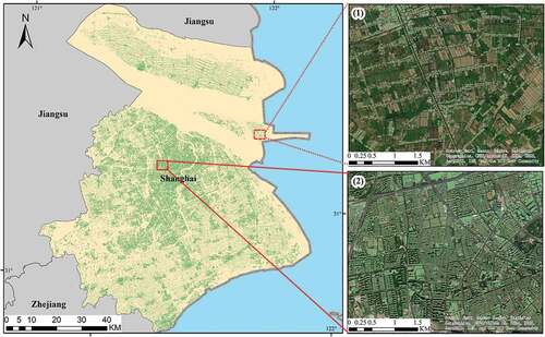
As shown in Figure 1, China was taken as the region of interest. China is located in the east of Asia and the west coast of the Pacific Ocean, covering a total area of about 9.6 million km². China is under a varied topography, and shows great diversity in physical geography, with mountainous areas, plateau, and hilly areas occupying two-thirds of the total land. The terrain of China slopes from west to east, forming a flight of three steps. The first step, i.e. region I step in Figure 1, which is the western part of the country, consists of the Qinghai-Xizang (Tibet) plateau with an elevation of over 4000 meters above sea level and is bounded by the Kunlun Qilian Mountains, Hengduan Mountains. The second step, i.e. region II step in Figure 1, includes the plateau and basin, generally at 1000–2000 m. The Great Hinggan Ridge–Mt. Taihang–Mt. Wushan–Mt. Xuefeng is located between the second step and the third step. The third step refers to the vast plains and hills of eastern China, with the altitude below 500 m, i.e. region III step in Figure 1.

Figure 1. Example images of buildings in both urban area and rural area from the three steps of China, respectively.

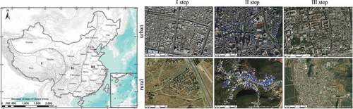
Due to the vast territory, complex natural environment, and different ethnic customs, buildings in different regions of China often have very different physiognomy and materiality. In addition, the surrounding natural environment can also have an impact on building identification. Forest vegetation and mountain rocks in geographically complex areas can easily be mistaken as buildings because they have high reflectance values and similar local textures, which usually lead to false positives.

As shown in Figure 1, in the first step, the roofs of buildings in the city are predominantly gray, and the floor area of the single building is relatively large. Most of the rural buildings are built along the mountains, and the single building occupies a small area and the buildings are sparsely distributed. In the second step, the roofs of buildings in the city are predominantly blue and gray, and the buildings are relatively scattered. Rural buildings are mostly located in the mountains, and the distribution is more concentrated. In the third step, the roofs of buildings in the city arise out of various colors, and the buildings are of different sizes and densely distributed. Rural buildings are mostly distributed on the plain, and the buildings are denser and more uniform than that of the other two steps.

4 Data

4.1 Data source and preprocessing

Remote sensing images and corresponding ground-truths used in this paper are of two kinds of spatial resolutions, i.e. 10 and 2.5 m. Figure 2 shows a sample from the city of Beijing, i.e. a 10=m Sentinel-2 image, a 2.5-m high-resolution image and their corresponding map of ground-truth building footprints, which are obtained from the Google Earth Engine (GEE) platform, 91 Satellite Map Assistant, and the building map from Tiandi Map and Open Street Map (OSM), respectively.

Figure 2. Demonstration of a Sentinel-2 image, a high-resolution image, and corresponding ground truth maps. (a) is the 10-m resolution true color image of Sentinel-2, (b) is the 10-m resolution ground truth map, (c) is the 2.5-m resolution image, and (d) is the 2.5 m resolution ground truth map of building footprints.

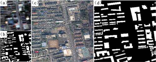
Sentinel-2 satellite has wide-range multi-spectral imaging capabilities with a global 5-day revisit frequency and can cover 13 spectral bands, including visible and near-infrared (NIR) bands at 10 m, red edge and short-wave infrared (SWIR) bands at 20 m, and atmospheric bands at 60-m spatial resolution. The images used in experiments are the Level-1C of Sentinel-2 with red, green, blue and near-infrared spectrum bands at 10 m resolution obtained from GEE platform. The images have been filtered to eliminate clouds and considering a maximum cloud cover of 20% of the scene, and preprocessed by splicing, de-clouding, and cropping.

High-resolution satellite images are utilized in experiments for manual verification of labels and comparison experiments. High-resolution satellite images are obtained from 91 Satellite Map Assistant, which is a satellite data download software. In 91 Satellite Map Assistant, the imagery is stitched from multiple satellite images. The image is divided into 20 levels, and the spatial resolution of each level is different. The spatial resolution of the 19-level image is about 0.3 m, and the 0-level image is about 135 km. To balance the image resolution with the download volume, images with a spatial resolution of 0.5 m were downloaded for each specific training region in this paper. Then, the images were down sampled using bicubic interpolation method to obtain the 2.5-m resolution data.

The ground truths of buildings are generated from building layer of Open Street Map (OSM) and Tiandi Map. For buildings on both OSM building layer and Tiandi Map, the building shapefiles from OSM are used because building annotations in it are more regular. And for buildings without both, the building outlines are drawn manually with high-resolution satellite images mentioned above. All building annotations are manual verified using 10-m sentinel-2 imagery and 2.5-m high-resolution imagery. Finally, the 10- and 2.5-m building semantic label maps are obtained by resampling and rasterization.

4.2 DREAM-A+ dataset

DREAM-A+ dataset is utilized to validate the performance of the proposed method. DREAM-A+ is an updated version of the DREAM-A dataset, which is a super-resolution semantic segmentation dataset in China originally constructed in Zhang et al. (2021), in which the data collection range is within China. However, there exist some drawbacks in the original dataset. (1) The dataset covers mainly the eastern and southeastern coastal cities, in which buildings are different from that in the north and west regions. (2) The dataset lacks some images samples with non-building areas, such as images with snow, clouds, fields, mountains, lakes, etc. (3) The original dataset only contains Sentinel-2 imagery, and lacks the corresponding high-resolution imagery, which make some comparison experiments unfeasible. (4) The ground truths of buildings in the original dataset are generated from building layer of Tiandi Map. Some of the building labels are of poor quality, and some non-building areas are incorrectly identified as buildings.

Taking into account the differences in the topography of each region, and the stylistic differences in buildings in different regions, seven cities in the west and north have been added in to the dataset, i.e. Harbin, Changchun, Hohhot, Xining, Lanzhou, Urumqi, and Linzhi. In order to reduce misidentification of non-building areas of model, non-building scenes such as clouds and snow, farmland, mountains, lakes, etc. have been added. High-resolution images and the ground truths of building footprints have been supplemented into the dataset as mentioned in Section 4.1.

Figure 3 shows the geographic location of DREAM-A+ dataset covering 38 cities in China. These images are grouped into three subsets according to the distribution of these cities. To meet the demands of the SRSS task, the lower resolution image tiles of size 64 × 64 and corresponding ground truths in the dataset share the same spatial resolution of 10 m, and the higher resolution tiles of size 256 × 256 are 2.5 m, as shown in Figure 2.

Figure 3. Distribution of DREAM-A+ Dataset. Red circle represents the distribution of training data. Blue square represents the distribution of testing data. Yellow color block represents the cities used for the qualitative analysis.

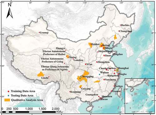
The first group, used to train and validate the models, contains 8583 image tiles from 31 cities and represents the situation of the major cities under different climates and landforms in China. The second group, including Chongqing, Wuhan, Qingdao, and Shanghai with approximately the same area, is utilized to quantitatively evaluate accuracy for extracting buildings based on the learned models. The size of each lower resolution image and corresponding ground truth is 1416 × 1437, and the higher resolution is 5664 × 5748. The third group, consisting of 10 cities, is used for qualitative analysis of the generalization ability of the learned model. The 10 cities can be divided into two levels: (1) Four municipalities directly under the central government (Beijing, Tianjin, Shanghai, and Chongqing). (2) Six cities representing different geographical divisions: Shenyang and Changsha in the northeast and east regions, Hohhot and Guiyang in the north and central regions, and Xining and Lhasa in the west and northwest.

5 Methods

In this paper, the models for super-resolution semantic segmentation are the same as the framework of ESPC_NASUnet (Penglei et al. 2021), which consists of two modules, i.e. SR and SS modules. As for the ESPC_NASUnet, it was validated on two high-resolution datasets, i.e. DREAM-B dataset with a resolution of 0.3 m (Yang and Tang 2020) and Massachusetts Buildings dataset with a resolution of 1 m (Mnih 2013), and the input data was obtained by 4× down sampling the high-resolution data using the Bicubic sampling method. It should be noted that for the task of building semantic segmentation, the spatial resolution of those two datasets after down sampling is high, and the information loss of the imagery is not significant. Therefore, the ESPC module, a simple structured SR module, is sufficient for the resolution improvement. However, the practicability of this method on real satellite images with medium-resolution remains to be verified. Considering the data cost and data scarcity of high-resolution data in large-scale building footprint mapping, it is a better choice to using a more efficient super-resolution semantic segmentation method for building footprints extraction from medium-resolution data. In this paper, we used the EDSR method which has deeper structure and better performance as a super-resolution module, and the proposed network is termed as EDSR_NASUnet.

5.1 EDSR_NASUnet

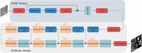
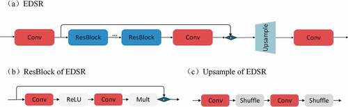
Figure 4 shows the modified end-to-end SRSS architecture in which the EDSR and NASUnet are used as SR and SS modules, respectively. In the EDSR module, 16 residual blocks are used. Lower resolution image with size of 64 × 64 is sent to the input layer. Then the EDSR module follows the input layer to obtain more detailed geometric information of buildings, which is important for efficiently reconstructing higher resolution features with size of 256 × 256. The NASUnet module receives the higher resolution features, compresses them in the spatial dimension via an encoder to a size of 8 × 8, and then is gradually restored to 256 × 256 via the decoder. In the end, we obtained the higher resolution semantic map with a size of 256 × 256 of buildings solely from lower resolution imagery.

Figure 4. The architecture of the proposed building super-resolution sematic segmentation method EDSR_NASUnet.

5.2 EDSR module

The EDSR is a simplified residual blocks from the SRResNet (Ledig et al. 2017) and can achieve significant performance improvement. Compared with the original ESPC module, the EDSR module has two main differences: (1) the feature extraction part is deeper and residual learning is added and (2) the spatial resolution enhancement of the feature no longer performs a one-time 4× up-sampling directly, but two 2× up-sampling. Figure 5(a) shows the architecture of the EDSR module. As shown in Figure 5(b), the adopted residual block (i.e. ResBlock) only contains convolutional layers and ReLU layer. Batch normalization layers in the original residual blocks are removed to increases the performance substantially (Nah, Hyun Kim, and Mu Lee 2017). The ReLU activation layers outside the residual blocks are also removed. The residual scaling with factor 0.1 is used to make the training procedure numerically stable. Sixteen ResBlocks are used in EDSR module. The input images are sent to convolutional layer and the ResBlocks for feature extraction. The obtained feature map is passed through up sampling layer to get super-resolution feature map. It is to be noted that the 4× up-sampling block is split into two 2× convolutions as shown in Figure 5(c), in order to reduce the loss of feature information caused by high magnification up-sampling at once.

Figure 5. The architecture of EDSR module. (a) is the architecture of EDSR module; (b) is the ResBlock of EDSR; (c) is the Up-sample of EDSR.

5.3 Experimental setting

5.3.1 Implementation details

In experiments, 3 NVIDIA K80 GPU is utilized to train the EDSR_NASUnet and other networks. The size of each input image is 64 × 64. Categorical cross entropy is used as the loss function. The optimizer Adaptive moment estimation, i.e. Adam (Kingma and Jimmy 2014), is applied to optimize the model parameters with a batch size of 16. The training period is set to 200. The initial learning rate is set to 1e-3. The learning rate decay method is exponential decay, and the decay coefficient is 0.98.

5.3.2 Evaluation metrics

In this paper, both pixel-level and object-level evaluation metrics are employed to evaluate the quantitative performance of the proposed and other deep learning models. Metrics in pixel-level evaluation include recall, precision, F1 Score, and kappa coefficient. Besides, intersection over union (IoU) is used, which is the ratio of the predicted building mask pixels and the mask pixels of ground truth intersection to their union:

(1) $IoU=\frac{Prediction\cap GroundTruth}{Prediction\cup GroundTruth}$(1)

The SRSS is a special task for building semantic segmentation in which the degree of separation of building objects is also important. Distinguishing two buildings that are several meters apart in an image with a spatial resolution of 10 m is indeed a challenge. In addition, in contrast to instance segmentation, the correspondence between predictions and building objects is always complex in SS. Therefore, three object-level metrics including Object-level Recall (OR), Object-level Precision (OP), and Object-level F1-score (OF1) are used to measure the degree of separation of building objects (Penglei et al. 2021). Interconnected predicted patches will be considered as one independent building object. For a target building mask, if an area of the prediction is close to the area of the actual building, the prediction is considered as a good result. However, if a real building is predicted to be many small building patches, such fragmentation results are unacceptable. This evaluation can be quantified by OR, which is given as follows for the $g$th building object $G{T}_g$:

(2) $O{R}_g=\frac{{\sum }_{i=1}^{n_g}{S}_{G{T}_g{\cap }^{p_i}}}{n_g{S}_{G{T}_g}}$(2)

where $n_g$ represents the number of predicted patches that intersect the $g$th building object, and $p_i$ is the $i$th patch of the predicted patches. $S$ is the area of the patch. Similarly, OP for the $h$th predicted patch is given as follows:

(3) $O{P}_h=\frac{{\sum }_{j=1}^{n_h}{S}_{p_h\cap G{T}_j}}{n_h{S}_{p_h}}$(3)

where $n_h$ represents the number of the real building objects that intersect the $h$th predicted patch, and $G{T}_j$ is the $j$th building object. Similar to the pixel metrics, OF1 is given as follows:

(4) $OF1=\frac{2\ast {\sum }_{g=1}^{m}O{R}_g\ast {\sum }_{h=1}^{n}O{P}_h}{n{\sum }_{g=1}^{m}O{R}_g+m{\sum }_{h=1}^{n}O{P}_h}$(4)

where m and n are the total quantities of building objects and the predicted patches, respectively.

5.3.3 Structures of SRSS networks for comparison

The proposed EDSR_NASUnet is trained with only lower resolution imagery to obtain the higher resolution semantic map. Most SRSS methods (Abadal et al. 2021) are not suitable for comparison, since they are trained with higher resolution imagery, and most of them have the scaling factor of 2, which is 4 in the proposed method. Therefore, the previous ESPC_NASUnet is chosen to compare with the proposed EDSR_NASUnet under the same conditions. Two recently proposed state-of-the-art SS methods, the HRnet (Sun et al. 2019) and DeepLab V3+ (Chen et al. 2018) of the DeepLab series, are used as two new SS module to compare. Four new SRSS networks, ESPC_HRnet, ESPC_DeepLab, EDSR_HRnet, and EDSR_DeepLab are utilized to compare with the proposed method.

6 Experimental results

In this section, both quantitative and qualitative comparisons of the proposed method and other end-to-end methods, e.g. ESPC_HRnet, ESPC_NASUnet, ESPC_DeepLab, EDSR_HRnet, and EDSR_DeepLab, are described in detail. Comparison between end-to-end SRSS method and stagewise SRSS methods is also conducted. Finally, the map of China’s building footprints is analyzed.

6.1 Performance of the SRSS methods

6.1.1 Quantitative evaluation

Table 2 lists the performance of the six different end-to-end SRSS networks in terms of five pixel-level metrics using data of the four cities for testing. The best performance of each metric has been highlighted with bold. The proposed EDSR_NASUnet method achieved the highest values among the six end-to-end SRSS networks in terms of the recall, F1-score, IoU, and kappa coefficient in Shanghai, Wuhan, and Chongqing. In Shanghai, the proposed EDSR_NASUnet method outperforms the remaining methods in terms of all metrics. It can be clearly seen from the above discussion that better performance statistics are obtained by the proposed EDSR_NASUnet.

Table 2. Pixel-level evaluation results.

Evaluation Region	Method	Pixel-level
		Recall	Precision	F1	IoU	Kappa
Qingdao	ESPC_HRnet	0.453	0.410	0.431	0.274	0.333
	ESPC_NASUnet	0.431	0.465	0.447	0.288	0.362
	ESPC_DEEPLAB	0.456	0.340	0.390	0.242	0.274
	EDSR_HRnet	0.486	0.472	0.479	0.315	0.393
	EDSR_NASUnet	0.505	0.448	0.475	0.311	0.384
	EDSR_DEEPLAB	0.399	0.477	0.435	0.278	0.352
Shanghai	ESPC_HRnet	0.607	0.621	0.614	0.443	0.503
	ESPC_NASUnet	0.533	0.660	0.590	0.418	0.486
	ESPC_DEEPLAB	0.507	0.541	0.524	0.355	0.391
	EDSR_HRnet	0.601	0.648	0.623	0.453	0.519
	EDSR_NASUnet	0.658	0.674	0.666	0.499	0.570
	EDSR_DEEPLAB	0.536	0.612	0.571	0.400	0.457
Wuhan	ESPC_HRnet	0.480	0.489	0.485	0.320	0.379
	ESPC_NASUnet	0.363	0.510	0.424	0.269	0.328
	ESPC_DEEPLAB	0.404	0.356	0.378	0.233	0.239
	EDSR_HRnet	0.479	0.494	0.487	0.322	0.382
	EDSR_NASUnet	0.502	0.483	0.493	0.327	0.384
	EDSR_DEEPLAB	0.417	0.476	0.445	0.286	0.338
Chongqing	ESPC_HRnet	0.453	0.495	0.473	0.310	0.378
	ESPC_NASUnet	0.390	0.557	0.459	0.298	0.377
	ESPC_DEEPLAB	0.412	0.411	0.412	0.259	0.300
	EDSR_HRnet	0.376	0.537	0.442	0.284	0.358
	EDSR_NASUnet	0.526	0.542	0.534	0.364	0.447
	EDSR_DEEPLAB	0.242	0.476	0.321	0.191	0.239

Note that the proposed method achieves the highest value of IoU in Shanghai, Wuhan, and Chongqing, i.e. 0.499, 0.327, and 0.364. In Qingdao, it differs from the optimal IOU value by only 0.004. This result demonstrates that the proposed method is more accurate in prediction of building footprints. However, all of the values of IoU are less than 0.5, which is pretty low in building extraction task. It is reasonable since the proposed method extracts the 2.5 m building footprint directly from the 10-m remote sensing imagery. Most individual buildings in the 10-m Sentinel-2 images are relatively smaller than those in high-resolution remote sensing images. The lower the resolution of the image, the fuzzier the building footprint is, and the more difficult the extraction is.

Compared with the ESPC module, each SS module coupled with EDSR module gets better performance, which indicates that the EDSR is more effective than the previous ESPC module. Compared with EDSR_HRnet and EDSR_DEEPLAB, the proposed EDSR_NASUnet also shows the outperformance on this Sentinel-2 dataset.

Table 3 presents the quantitative evaluations generated by the six different end-to-end SRSS networks using three object-level metrics. The best performance of each metric has been highlighted with bold. The proposed EDSR_NASUnet method outperformed other models in terms of both OR and OF1 on object-level. Compared with the ESPC module, each SS module with EDSR module achieves better performance on object-level evaluation, which indicates that the improved EDSR is more effective than the previous ESPC module in extracting building footprints from Sentinel-2 images. Compared with EDSR_HRnet and EDSR_DEEPLAB, EDSR_NASUnet gets the highest OR and lower OP, which means the network tends to predict an integrated patch to approximate the true building patch, that is, it predicts with low fragmentation. The highest value of OF1 indicates the EDSR_NASUnet achieves a better balance between too many fragments and over-adhesion in building footprint prediction compared with the other SRSS methods.

Table 3. Object-level evaluation results.

Method	Object-level
	OR	OP	OF1
ESPC_HRnet	0.401	0.376	0.388
ESPC_NASUnet	0.336	0.435	0.377
ESPC_DEEPLAB	0.349	0.356	0.351
EDSR_HRnet	0.405	0.445	0.424
EDSR_NASUnet	0.446	0.417	0.431
EDSR_DEEPLAB	0.358	0.446	0.397

6.1.2 Qualitative evaluation

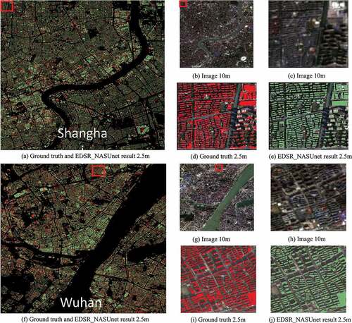
Figure 6 shows the results of building identification within Shanghai and Wuhan. It can be seen that the EDSR_NASUnet can well recognize individual buildings from combining both feature super-resolution and semantic segmentation. As shown in Figure 6(e-j), some small size houses and densely distributed individual buildings are clearly recognized with approximation building contours. The results confirmed that the EDSR_NASUnet is feasible to generate building footprints from medium-resolution images, i.e. Sentinel-2 images.

Figure 6. The building extraction results in Shanghai and Wuhan. (a) and (f) respectively represent the overlay of identification result (green color) on the ground truth (red color) of Shanghai and Wuhan at 2.5 m, where (b) and (g) are the corresponding Sentinel-2 images at 10 m resolution. (c–e) and (h–j) are the enlarged display of the small area in the red box of (a) and (f), respectively.

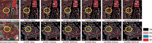
Figure 7 shows the identification results of six end-to-end SRSS methods from Sentinel-2 images within Shanghai and Wuhan. As shown in Figure 7(a-g), the buildings on the left in the image are relatively small objects and are accurately identified. But the buildings within the yellow circle are not well recognized, especially ESPC_DEEPLAB. In Figure 7(h-n), the recognition results of the image within Wuhan are generally poor relative to Shanghai. Within the yellow circles, only EDSR_NASUnet accurately identifies the building with red roof. ESPC_HRnet and EDSR_HRnet misclassify non-buildings into buildings relatively seriously. On the right side of the figures, only EDSR_NASUnet is relatively accurate in their predictions, other networks misclassify the buildings into backgrounds. While EDSR_NASUnet identifies buildings more completely, it identifies multiple adjacent buildings as one building. Overall, the EDSR_NASUnet method can generate a semantic map with fewer omissions and a better approximation to the edges of building.

Figure 7. Visual examples of predicted buildings of six end-to-end SRSS methods from a Sentinel-2 image in Shanghai and Wuhan. Red blocks are ground truth of buildings with 2.5 m resolution. The FNs, FPs, and TPs are exhibited in pink, blue, and red colors, respectively.

The above comparisons demonstrate the superiority of the proposed EDSR_NASUnet from both quantitative and qualitative perspectives.

6.2 Comparison between EDSR_NASUnet and stagewise methods

For better understanding the effectiveness of proposed method, i.e. EDSR_NASUnet, stage-wise SRSS methods with four modes are tested on the DREAM-A+ datasets. As shown in Table 4, instead of training the SS(HRI) network with HR images in the first mode, i.e. SR+SS(HRI), the SS(SRI) network in the second mode, i.e. SR+SS(SRI) is trained with images generated by the SR networks, e.g. ESPCN or EDSR. Nearest Resampling the results of SS(LRI) is used as the postprocess in the third mode, i.e. SS(LRI)+Nearest. In the last mode, LR images and corresponding LR GT are used to train the SS(LRI) models. The HR GT is used in SR training process with the probability map of buildings generated by the SS(LRI) networks.

Table 4. General settings of stage-wise methods.

Mode	SR Training data	SS Training data	Test data	Preprocessing	Post-Processing
SR+SS(HRI)	LR images+HR images	HR images+HR GT	LR images	Image SR	-
SR+SS(SRI)	LR images+HR images	SR images+HR GT	LR images	Image SR	-
SS(LRI)+Nearest	-	LR images+LR GT	LR images	-	Nearest Resampling
SS(LRI)+SR	LR probability map+HR GT	LR images+LR GT	LR images	-	Probability map SR

As shown in Table 5, the SR+SS (SRI) mode get better performance among the four modes. Compared with the independently trained SR and SS network in SR+SS (HRI) mode, SS(SRI) trained on the basis of SR-preprocessed data can extract buildings more effectively from the test data after SR processing. In other words, when two independent networks are collaborative in the data level, the performance of the stagewise method will be better than that of the completely independent networks method. In contrast, the SS(LRI)+SR mode performs inconsistent. When training the SR network, the probability map has lost the original information compared with the input image. Besides, the poorly performance of SS(LRI) network directly misleads the training of the SR network afterward. The proposed EDSR_NASUnet get much better values of most metrics, which means EDSR_NASUnet works better on building footprint recognition from lower resolution imagery, especially on small buildings. Compared with the SR+SS(HRI) mode, EDSR_NASUnet gets lower pixel-level precision, since the input data with lower resolution of the SRSS has partially indistinguishable or non-separable buildings. On the object-level, the OR of EDSR_NASUnet is higher, but the OP is lower, indicating that the network predicts with higher fragmentation than the prediction generated from the 2.5 m-resolution imagery.

Table 5. Evaluation Results of stage-wise SRSS methods and EDSR_NASUnet.

Stage-wise SRSS Methods		Recall	Precision	F1-score	mIoU	Kappa	OR	OP	OF1
SR+SS（HRI）	ESPCN + UNASNetMobile	0.018	0.643	0.035	0.422	0.026	0.010	0.535	0.020
	ESPCN + DeepLab V3+	0.049	0.601	0.091	0.437	0.066	0.033	0.500	0.061
	EDSR + UNASNetMobile	0.181	0.591	0.278	0.496	0.213	0.150	0.500	0.231
	EDSR + DeepLab V3+	0.205	0.586	0.304	0.505	0.235	0.165	0.484	0.246
SR+SS (SRI)	ESPCN+UNASNetMobile	0.420	0.308	0.355	0.465	0.193	0.327	0.395	0.358
	ESPCN+DeepLab V3+	0.480	0.488	0.484	0.562	0.376	0.378	0.410	0.393
	EDSR+UNASNetMobile	0.446	0.453	0.449	0.542	0.334	0.353	0.421	0.384
	EDSR+DeepLab V3+	0.337	0.598	0.431	0.555	0.349	0.255	0.515	0.341
SS(LRI)+Nearest	UNASNetMobile	0.181	0.491	0.264	0.486	0.188	0.129	0.349	0.189
	DeepLab V3+	0.230	0.487	0.312	0.501	0.225	0.160	0.312	0.211
SS(LRI)+SR	UNASNetMobile + ESPCN	0.181	0.507	0.267	0.487	0.193	0.010	0.535	0.020
	DeepLab V3+ + ESPCN	0.232	0.505	0.318	0.504	0.234	0.124	0.388	0.188
	UNASNetMobile + EDSR	0.000	0.000	0.000	0.413	0.000	0.000	0.000	0.000
	DeepLab V3+ + EDSR	0.260	0.461	0.333	0.504	0.237	0.165	0.484	0.246
EDSR_NASUnet		0.559	0.547	0.553	0.604	0.457	0.446	0.417	0.431

6.3 Building footprint mapping in China

6.3.1 Buildings distribution in China

The footprint area of buildings in China in 2019 is shown in Figure 8, which is calculated based on the 2.5 m identification results of the EDSR_NASUnet. To better show the distribution of buildings across the country, we counted the distribution of building areas within a 0.41- by 0.31-degree latitude/longitude grid. The green Aihui-Tengchong line in Figure 8 divides China into two parts. According to the sixth national census in 2010, about 93.68% of the population lives in about 43.8% of the land in the southeast of the line, and the population density in the northwest of the line is extremely low. In other words, the law of population distribution revealed by the Aihui-Tengchong line is still valid in China. It can be seen from Figure 8 that most buildings are located on the southeast side of this line, with significantly fewer buildings on the northwest side. We calculated the building footprint area on both sides of the Aihui-Tengchong line. The building footprint area on the southeast side is 889,055.62 km², while on the northwest side it is 230,481.78 km². The building footprint area of the southeast side of the Aihui-Tengchong line is about 3.9 times that of the northwest side, which accounts for 79% of the whole national area.

Figure 8. Map of China building footprint distribution in 2019.

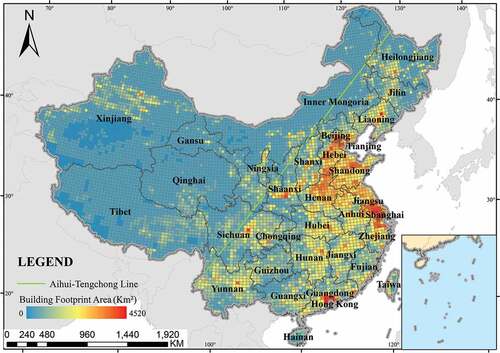
The most densely built-up areas in the country are mainly concentrated in the North China Plain, the Yangtze River Delta and Guangdong-Hong Kong-Macao Greater Bay Area. The cities with the highest building area are mainly distributed in the third step of China’s terrain such as Beijing, Shanghai, and Guangzhou, while the areas with the highest building density in each province are mostly located in provincial capital cities, which also reveals that building density is closely related to the economy.

The whole prediction process of China building footprints is finished on GEE platform, Google Drive, and Google Colaboratory. It took about 221.9 hours to download the data from GEE platform to Google Drive, and 166.43 hours to predict the building footprints using P100 on Google Colaboratory. This is pretty efficient for making national-scale building footprint products.

6.3.2 Buildings distribution in municipalities

Figures 9 and 10 respectively show the distribution of buildings in two municipalities directly under the central government, i.e. Beijing and Chongqing, where the green blocks are the building footprints obtained from the EDSR_NASUnet model. Sub figures (1) and (2), which are located at the red boxes, are the distribution of buildings in the suburb and city center, respectively.

Figure 9. Building footprints in Beijing. Sub figures (1) and (2) represent the building footprints in suburb and city center, respectively.

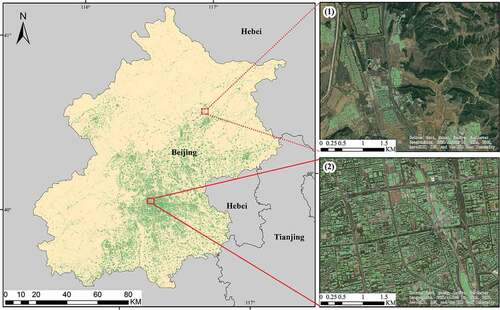
Figure 10. Building footprints in Chongqing. The subfigure (1) and (2) represent the building footprints in suburb and city center, respectively.

As revealed in each figure, the buildings are densely distributed in the city center, and the building density is getting lower and lower toward the city’s edge. In the city center, there are many large buildings, and the distribution of the buildings is dense and regular. The generated building footprints can be well generalized. The buildings in the suburbs are smaller, more clustered in a small area, and more scattered on the whole. The generated building footprints basically cover the area where the building is located on the image. But some buildings were not well identified. This may be due to the lower reflectance values of buildings and similar spectral signatures of different types of objects in the suburbs.

6.3.3 Buildings distribution in cities

We have selected and presented the identification results of three cities representing different geographical divisions: Shenyang in the third step of China’s terrain, Guiyang in the second step of China’s terrain, and Xining in the first step of China’s terrain. Figure 11 shows the detail of building footprints. The green blocks represent the results of building footprints generated from the EDSR_NASUnet model.

Figure 11. Building footprints in Shenyang, Guiyang, and Xining. The right subfigure is the enlarged display of a local small area in the red box of the left subfigure.

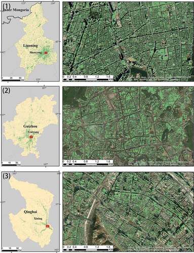
As shown in Figure 11, the results show that the learned models can be well generalized to some cities in the east regions of China. Buildings in these cities are of large size, densely distributed, and arranged in order. However, for some cities, e.g. Xining, the results are not as good as other cities. This may be due to the high reflectance values of non-buildings, since they are located on the plateau and grassland Gobi, the land surface of these regions is very different from the east regions.

7 Discussion

7.1 Preliminary analysis

In this paper, the aim of the building recognition is to obtain HR semantic maps of buildings from LR images, which assumes that each individual building is distinguishable from its surrounding non-building on low-resolution images. That is to say that there exists a difference in reflectance value inside and outside the building boundaries on Sentinel-2 image. In order to verify the assumption, we evaluated the differences of the buildings and non-buildings in Sentinel 2 images by using both quantitative and qualitative evaluation approaches.

7.1.1 Quantitative evaluation

As for each building in an image, to measure the difference in reflectance values between buildings and non-buildings, we calculate the Jensen–Shannon divergence (JS divergence) between this building and the corresponding neighboring non-buildings in terms of the distribution of reflectance values. The JS divergence is usually used to measure the similarity between two probability distributions in many applications, such as sensor data fusion (Xiao 2018), and machine learning (Goodfellow 2016), and it is bounded by 0 and 1. The higher the value, the less similar the two distributions are. We use the JS divergence of the corresponding 2.5-m images as the upper bound for the separability of buildings and non-buildings in the Sentinel-2 images. The JS divergence can be calculated by:

(5) $KL(P||Q)={\sum }_{i}P\left(i\right)ln\frac{P\left(i\right)}{Q\left(i\right)}$(5)

$JS(P_1||P_2)=\frac{1}{2}KL(P_1||\frac{P_1+P_2}{2})$+ $\frac{1}{2}KL(P_2||\frac{P_1+P_2}{2})$ (6)

where P(i) and Q(i) are the probability distributions, respectively, and the 1/2(P₁ + P₂) is the mixture distribution of P₁ and P₂. JS divergence of two distributions is between 0 and 1. The closer the value is to 0, the lower the separability of the two distributions, and the higher the contrary.

To better characterize the differences in reflectance values between buildings and non-buildings on Sentinel 2 images, we chose all of the training images in DREAM-A+ Dataset. Two approaches were chosen to select building and non-building regions in this paper.

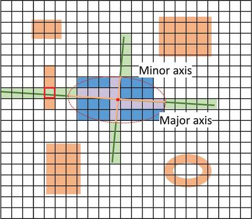
The first approach is shown in Figure 12, where each building has a corresponding ellipse, which has the same normalized second central moments. We collected the reflectance values with the same length of the major-axis in the major-axis direction of corresponding ellipse of the building, and those in the minor-axis direction. If there exists a pixel belonging to a building, which is not the target building, the reflectance value of this pixel will be excluded. As shown in Figure 12, the black grid represents the pixel grid of the image, and the blue and orange blocks represent the building footprints in the corresponding areas. The blue color blocks represent the buildings of interest. The red ellipse is the corresponding ellipse, and the orange lines are the major axis and minor axis. The reflectance values in green blocks are the reflectance values of non-buildings. Please note that the reflectance values in in the red square box are not recorded. The reflectance values in mauve blocks are the reflectance values of interest building.

Figure 12. The process of reflectance value collection with main axis of the ellipse that has the same normalized second central moments as the building region. The black grid represents the pixel grid of the image and the color blocks represent the building footprints in the corresponding areas. The blue color blocks represent the buildings of interest. The red ellipse is the corresponding ellipse, and the orange lines are the major axis and minor axis.

Table 6 lists the JS divergence of buildings and non-buildings on different bands. The JS divergence of Sentinel-2 shows that there exists a difference in reflectance values between buildings and non-buildings on Sentinel-2. In particular, the value of JS divergence gets highest scores on red band on both Sentinel-2 and 2.5-m resolution imagery, which means the differentiability of buildings and non-buildings is greater on the red band among those bands.

Table 6. JS divergence of buildings and non-buildings on axis.

Image	Axis	Blue band	Green band	Red band	NIR band
Sentinel-2	Minor axis	0.074	0.082	0.118	0.110
	Major axis	0.072	0.066	0.115	0.121
2.5m Image	Minor axis	0.188	0.192	0.227	-
	Major axis	0.157	0.120	0.200	-

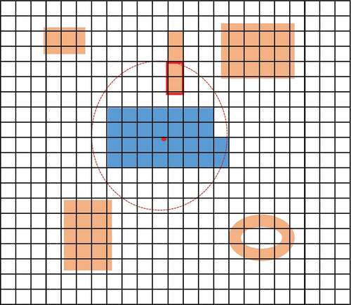
The second approach is shown in Figure 13, where a circle is drawn with the center point of each building as the center and five pixels as the radius. The black grid represents the pixel grid of the image and the color blocks represent the building footprints in the corresponding areas. The blue color blocks represent the buildings of interest. The reflectance values of the non-building area pixels within the circle are collected as the reflectance distribution of non-buildings (the reflectance of pixels in red box will not be recorded), and the reflectance values in blue blocks are the reflectance values of interest building.

Figure 13. The process of reflectance value collection with a circle. The black grid represents the pixel grid of the image and the color blocks represent the building footprints in the corresponding areas. The blue color blocks represent the buildings of interest. The red circle is the corresponding circle.

Table 7 shows the JS divergence of buildings and non-buildings on different bands. The JS divergence of Sentinel-2 also shows that single building is distinguishable from its surrounding non-building on Sentinel 2. Compared with JS divergences in Table 6, JS divergences on different bands on Sentinel-2 are bigger, and the differences between Sentinel-2 images and the 2.5-m resolution images are smaller. This may be due to the greater range of reflectance of building and its surrounding non-building.

Table 7. JS divergence of buildings and non-buildings within circle.

Image	Blue band	Green band	Red band	NIR band
Sentinel-2	0.137	0.160	0.245	0.251
2.5m Image	0.192	0.199	0.245	-

7.1.2 Qualitative evaluation

To more intuitively observe the difference between building and its surrounding non-building on reflectance values, a Sentinel-2 image was taken as an example, which is shown in Figure 14. The distribution of reflectance values in the west–east direction and in the north–south direction is plotted in Figure 14(b,c), respectively. The left is the reflectance distribution in the west-east direction, and the right one is in the north–south direction, as marked with red lines in Figure 14. The blue bins represent the buildings, and the red ones represent the non-buildings.

Figure 14. A Sentinel-2 image in Beijing and the reflectance values of the red line on the Sentinel-2 image. (a) is the Sentinel-2 image. (b) and (c) are the reflectance values from west to east and from north to south, respectively. From top to bottom are the labels of the buildings in the corresponding area, the reflectance on the blue, green, red, and near-infrared band. The red bins represent reflectance values of non-buildings, and the blue bins represent reflectance values of buildings.

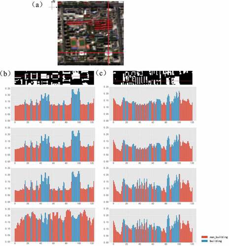
Obviously, there exists a certain difference in reflectance between buildings and non-buildings, with most buildings having higher reflectance values than the surrounding non-buildings in the blue, green, and red bands, especially the red band. Differences are not significant in the near-infrared band.

7.2 Comparison with other production using Sentinel images

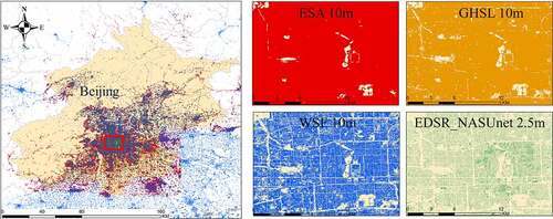
In Beijing city, our results and three products, i.e. from ESA (Zanaga et al. 2021), GHSL (Corbane et al. 2021), and WSF (Marconcini et al. 2020), are shown in Figure 15, which are produced from 10-m Sentinel-2 images using different approaches. Individual buildings cannot be discriminated in the products of both ESA and GHSL. Although districts can be well separated in the WSF product, individual buildings cannot be well identified. In contrast, individual buildings with a same district can be well separated and correctly identified in our results.

Figure 15. Map of building footprints in Beijing. The red, yellow, blue, and green maps represent the map of buildings generated by ESA, GHSL, WSF, and the proposed EDSR_NASUnet method, respectively. All of them are generated from Sentinel-2 images with 10 m resolution.

8 Conclusion

Although very high spatial resolution (VHR) remote sensing images have been often utilized to validate the effectiveness in terms of buildings mapping, national-scale of VHR building footprint products is relatively lacking in China due to limited data availability. With the open access to high frequency revisit Sentinel-2 remote sensing imagery, this paper proposes an end-to-end super-resolution semantic segmentation method, which extracts buildings through feature super-resolution of medium-resolution images combined with semantic segmentation. The main conclusions are as follows:

1. An improved model for feature super-resolution semantic segmentation is proposed in this paper. Unlike ESPC_NASUnet for down-sampling images, the improved model is designed for a real scenario, i.e. 10-m Sentinel-2 images and 2.5 ground-truths, which consists of a more complex feature super-resolution model, i.e. EDSR. As the resolution of the remote sensing imagery decreases, the building footprint becomes fuzzier, which brings a big challenge to building identification. The more complex super-resolution module is helpful to improve the building recognition results of medium-resolution remote sensing images.

2. From both quantitative and qualitative aspects, we validated the potential for Sentinel-2 data to discriminate single buildings, which provides an effective way to extract large-scale building footprints from low-resolution remote sensing images with great advantage of being free and having a high revisit frequency.

3. The proposed model was used to generate 2.5-m semantic map of building footprint with the real remote sensing imagery of Sentinel-2 in the China. To the authors’ knowledge, this is the first time that a China-wide building footprint product has been completed using single data source, and the accuracy of the product is close to that with multi-source data. Over 86.3 million individual buildings are detected with a total rooftop area of buildings of approximately 58,719.43 km². The number of buildings increased from 5.73 million Ain the first step of China’s terrain, through 23.41 million in the second step of China’s terrain, to 57.16 million in the third step of China’s terrain. The area of buildings also increased from 3318.02 through 13,844.29 to 41,557.12 km². In addition, the results show that the distribution of buildings varies greatly across China, and that the distribution density of buildings matches well with the relationship with the Aihui-Tengchong line, which characterizes population density.

Since the proposed method relies on freely available satellite imagery and open-source platforms, which allows us to update the map frequently and at a low cost. This work might also stimulate potential large-scale application related to human activities. In future work, we will focus on improving the extraction performance of small buildings and buildings in rural areas. We might extend it to map individual buildings in a wider region and within a narrower time interval.

Acknowledgments

This work was supported in part by the National Natural Science Foundation of China under Grant 42192584 and 41971280.

Disclosure statement

The authors declare that they have no known competing financial interests or personal relationships that could have appeared to influence the work reported in this paper.

Data availability statement

The data of the footprint of buildings in China 2019 is available at https://code.earthengine.google.com/?asset=users/flower/2019_China. The dataset presented in this study is available on request from the corresponding author.

Additional information

Funding

The work was supported by the National Natural Science Foundation of China [42192584, 41971280].

References

- Abadal, S., L. Salgueiro, J. Marcello, and V. Vilaplana. 2021. “A Dual Network for Super-Resolution and Semantic Segmentation of Sentinel-2 Imagery.” Remote Sensing 13 (22): 4547. doi:10.3390/rs13224547.
- Ayala, C., C. Aranda, and M. Galar. 2021. “Multi-Class Strategies for Joint Building Footprint and Road Detection in Remote Sensing.” Applied Sciences 11 (18): 8340. doi:10.3390/app11188340.
- Balk, D. L., U. Deichmann, G. Yetman, F. Pozzi, S. I. Hay, and A. Nelson. 2006. “Determining Global Population Distribution: Methods, Applications and Data.” Advances in Parasitology 119–22. doi:10.1016/s0065-308x(05)62004-0.
- Bartholomé, E., and A. S. Belward. 2005. “GLC2000: A New Approach to Global Land Cover Mapping from Earth Observation Data.” International Journal of Remote Sensing 26 (9): 1959–1977. doi:10.1080/01431160412331291297.
- Benjamin, S., H. L. Y. Melanie Laverdiere, A. Rose, and A. Rose. 2022. “Iterative Self-Organizing SCEne-LEvel Sampling (ISOSCELES) for Large-Scale Building Extraction.” GIScience & Remote Sensing 59 (1): 1–16. doi:10.1080/15481603.2021.2006433.
- Bicheron, P., V. Amberg, L. Bourg, D. Petit, M. Huc, Miras, B., Brockmann, C., et al. 2011 . “Geolocation Assessment of MERIS GlobCover Orthorectified Products.” Geoscience and Remote Sensing, IEEE Transactions on 49 2972–2982 doi:10.1109/TGRS.2011.2122337 .
- Brown, C. F., S. P. Brumby, B. Guzder-Williams, T. Birch, S. Brooks Hyde, J. Mazzariello, W. Czerwinski, et al. 2022. “Dynamic World, Near Real-Time Global 10 m Land Use Land Cover Mapping.” Scientific Data 9 (1): 251. doi:10.1038/s41597-022-01307-4.
- Chen, J., J. Chen, A. Liao, X. Cao, L. Chen, X. Chen, H. Chaoying, et al. 2015. “Global Land Cover Mapping at 30m Resolution: A POK-Based Operational Approach.” ISPRS Journal of Photogrammetry and Remote Sensing 103 (May): 7–27. doi:10.1016/j.isprsjprs.2014.09.002.
- Chen, J., P. Gong, H. Chunyang, W. Luo, M. Tamura, and P. Shi. 2002. “Assessment of the Urban Development Plan of Beijing by Using a CA-Based Urban Growth Model.” Photogrammetric Engineering and Remote Sensing 68: 1063–1072.
- Chen, L.C., G. Papandreou, I. Kokkinos, K. Murphy, and A. L. Yuille. 2018. “DeepLab: Semantic Image Segmentation with Deep Convolutional Nets, Atrous Convolution, and Fully Connected CRFs.” IEEE Transactions on Pattern Analysis and Machine Intelligence 40 (4): 834–848. doi:10.1109/TPAMI.2017.2699184.
- Corbane, C., V. Syrris, F. Sabo, P. Politis, M. Melchiorri, M. Pesaresi, P. Soille, and T. Kemper. 2021. “Convolutional Neural Networks for Global Human Settlements Mapping from Sentinel-2 Satellite Imagery.” Neural Computing & Applications 33 (12): 6697–6720. doi:10.1007/s00521-020-05449-7.
- Dixit, Mayank, Kuldeep Chaurasia, and Vipul Kumar Mishra. 2021. “Dilated-ResUnet: A Novel Deep Learning Architecture for Building Extraction from Medium Resolution Multi-Spectral Satellite Imagery.” Expert Systems with Applications 184 (December): 115530. doi:10.1016/j.eswa.2021.115530.
- Dong, C., C. Change Loy, H. Kaiming, and X. Tang. 2014. “Learning a Deep Convolutional Network for Image Super-Resolution.” In European Conference on Computer Vision, Zurich, Switzerland. September 6-12, 2014; 8692: 184–199. Springer, Cham. doi:10.1007/978-3-319-10593-2_13.
- Elvidge, C. D., M. L. Imhoff, K. E. Baugh, V. Ruth Hobson, I. Nelson, J. Safran, J. B. Dietz, and B. T. Tuttle. 2001. “Night-Time Lights of the World: 1994–1995.” ISPRS Journal of Photogrammetry and Remote Sensing 56 (2): 81–99. doi:10.1016/S0924-2716(01)00040-5.
- Elvidge, C., B. Tuttle, P. Sutton, K. Baugh, A. Howard, C. Milesi, B. Bhaduri, and R. Nemani. 2007. “Global Distribution and Density of Constructed Impervious Surfaces.” Sensors 7 (9): 1962–1979. doi:10.3390/s7091962.
- Esch, T., M. Marconcini, A. Felbier, A. Roth, W. Heldens, M. Huber, M. Schwinger, H. Taubenbock, A. Muller, and S. Dech. 2013. “Urban Footprint Processor—fully Automated Processing Chain Generating Settlement Masks from Global Data of the TanDEM-X Mission.” IEEE Geoscience and Remote Sensing Letters 10 (6): 1617–1621. doi:10.1109/LGRS.2013.2272953.
- Friedl, M. A., D. K. McIver, J. C. F. Hodges, X. Y. Zhang, D. Muchoney, A. H. Strahler, C. E. Woodcock, et al. 2002. “Global Land Cover Mapping from MODIS: Algorithms and Early Results.” Remote Sensing of Environment 83 (1–2): 287–302. doi:10.1016/S0034-4257(02)00078-0.
- Frolking, Steve, Tom Milliman, Karen C Seto, and Mark A Friedl. 2013. “A Global Fingerprint of Macro-Scale Changes in Urban Structure from 1999 to 2009.” Environmental Research Letters 8 (2): 024004. doi:10.1088/1748-9326/8/2/024004.
- Gong, P., H. Liu, M. Zhang, L. Congcong, J. Wang, H. Huang, N. Clinton, et al. 2019. “Stable Classification with Limited Sample: Transferring a 30-M Resolution Sample Set Collected in 2015 to Mapping 10-M Resolution Global Land Cover in 2017.” Science Bulletin 64 (6): 370–373. doi:10.1016/j.scib.2019.03.002.
- Gong, P., J. Wang, Y. Le, Y. Zhao, Y. Zhao, L. Liang, Z. Niu, et al. 2013. “Finer Resolution Observation and Monitoring of Global Land Cover: First Mapping Results with Landsat TM and ETM+ Data.” International Journal of Remote Sensing 34 (7): 2607–2654. doi:10.1080/01431161.2012.748992.
- Guangming, W., Z. Guo, X. Shi, Q. Chen, X. Yongwei, R. Shibasaki, and X. Shao. 2018. “A Boundary Regulated Network for Accurate Roof Segmentation and Outline Extraction.” Remote Sensing 10 (8): 1195. doi:10.3390/rs10081195.
- Guo, Z., W. Guangming, X. Song, W. Yuan, Q. Chen, H. Zhang, X. Shi, et al. 2019. “Super-Resolution Integrated Building Semantic Segmentation for Multi-Source Remote Sensing Imagery.” IEEE Access 7: 99381–99397. doi:10.1109/ACCESS.2019.2928646.
- Hansen, M. C., R. S. DeFries, J. R. Townshend, and R. Sohlberg. 2000. “Global Land Cover Classification at 1 Km Spatial Resolution Using a Classification Tree Approach.” International Journal of Remote Sensing 21 (6–7): 1331–1364. doi:10.1080/014311600210209.
- Hasan, N., M. Shukor, and A. J. Ghandour. 2023. “Sci-Net: Scale Invariant Model for Buildings Segmentation from Aerial Imagery.” Signal, Image and Video Processing, 1–9. doi:10.1007/s11760-023-02520-3.
- Heipke, C. 2010. “Crowdsourcing Geospatial Data.” ISPRS Journal of Photogrammetry and Remote Sensing 65 (6): 550–557. doi:10.1016/j.isprsjprs.2010.06.005.
- Homer, C., C. Huang, L. Yang, B. Wylie, and M. Coan. 2004. “Development of a 2001 National Land-Cover Database for the United States.” Photogrammetric Engineering & Remote Sensing 70 (7): 829–840. doi:10.14358/PERS.70.7.829.
- Huang, X., D. Wen, L. Jiayi, and R. Qin. 2017. “Multi-Level Monitoring of Subtle Urban Changes for the Megacities of China Using High-Resolution Multi-View Satellite Imagery.” Remote Sensing of Environment 196 (July): 56–75. doi:10.1016/j.rse.2017.05.001.
- Jiayi, L., X. Huang, T. Lilin, T. Zhang, and L. Wang. 2022. “A Review of Building Detection from Very High Resolution Optical Remote Sensing Images.” GIScience & Remote Sensing 59 (1): 1199–1225. doi:10.1080/15481603.2022.2101727.
- Karra, K., C. Kontgis, Z. Statman-Weil, J. C. Mazzariello, M. Mathis, and S. P. Brumby. 2021. “Global Land Use/Land Cover with Sentinel 2 and Deep Learning.” In 2021 IEEE International Geoscience and Remote Sensing Symposium IGARSS, 4704–4707. IEEE. 10.1109/IGARSS47720.2021.9553499.
- Khoshboresh-Masouleh, M., and R. Shah-Hosseini. 2021. “Building Panoptic Change Segmentation with the Use of Uncertainty Estimation in Squeeze-And-Attention CNN and Remote Sensing Observations.” International Journal of Remote Sensing 42 (20): 7798–7820. doi:10.1080/01431161.2021.1966853.
- Kingma, D. P., and B. Jimmy. (2014). “Adam: A Method for Stochastic Optimization .” ArXiv E-Prints, December, arXiv:1412.6980. doi:10.48550/arXiv.1412.6980.
- Kriti, R., P. Bodani, and S. A. Sharma. 2022. “Automatic Building Footprint Extraction from Very High-Resolution Imagery Using Deep Learning Techniques.” Geocarto International 37 (5): 1501–1513. doi:10.1080/10106049.2020.1778100.
- Ledig, C., L. Theis, F. Huszar, J. Caballero, A. Cunningham, A. Acosta, A. Aitken, et al. 2017. “Photo-Realistic Single Image Super-Resolution Using a Generative Adversarial Network.” In 2017 IEEE Conference on Computer Vision and Pattern Recognition (CVPR), 105–114. 10.1109/CVPR.2017.19.
- Liu, Y., D. Minh Nguyen, N. Deligiannis, W. Ding, and A. Munteanu. 2017. “Hourglass-ShapeNetwork Based Semantic Segmentation for High Resolution Aerial Imagery.” Remote Sensing 9 (6): 522. doi:10.3390/rs9060522.
- Loveland, T. R., and A. S. Belward. 1997. “The International Geosphere Biosphere Programme Data and Information System Global Land Cover Data Set (DISCover).” Acta Astronautica 41 (4–10): 681–689. doi:10.1016/S0094-5765(98)00050-2.
- Luo, X., X. Tong, Z. Qian, H. Pan, and S. Liu. 2019. “Detecting Urban Ecological Land-Cover Structure Using Remotely Sensed Imagery: A Multi-Area Study Focusing on Metropolitan Inner Cities.” International Journal of Applied Earth Observation and Geoinformation 75 (March): 106–117. doi:10.1016/j.jag.2018.10.014.
- Maggiori, E., Y. Tarabalka, G. Charpiat, and P. Alliez. 2017. “Convolutional Neural Networks for Large-Scale Remote-Sensing Image Classification.” IEEE Transactions on Geoscience and Remote Sensing 55 (2): 645–657. doi:10.1109/TGRS.2016.2612821.
- Marconcini, M., A. Metz-Marconcini, T. Esch, and N. Gorelick. 2021. “Understanding Current Trends in Global Urbanisation - the World Settlement Footprint Suite.” GI_Forum 1: 33–38. doi:10.1553/giscience2021_01_s33.
- Marconcini, M., A. Metz-Marconcini, S. Üreyen, D. Palacios-Lopez, W. Hanke, F. Bachofer, J. Zeidler, et al. 2020. “Outlining Where Humans Live, the World Settlement Footprint 2015.” Scientific Data 7 (1): 242. doi:10.1038/s41597-020-00580-5.
- Mnih, V. 2013. Machine Learning for Aerial Image Labeling. University of Toronto, Canada: University of Toronto (Canada). ISBN:978-0-494-96184-1.
- Nah, S., T. Hyun Kim, and K. Mu Lee. 2017. “Deep Multi-Scale Convolutional Neural Network for Dynamic Scene Deblurring.” In Proceedings of the IEEE Conference on Computer Vision and Pattern Recognition, 257–265. Honolulu, HI, USA, doi:10.1109/CVPR.2017.35.
- Okolie, C. J., and J. L. Smit. 2022. “A Systematic Review and Meta-Analysis of Digital Elevation Model (DEM) Fusion: Pre-Processing, Methods and Applications.” ISPRS Journal of Photogrammetry and Remote Sensing 188 (June): 1–29. doi:https://doi.org/10.1016/j.isprsjprs.2022.03.016.
- Penglei, X., H. Tang, G. Jiayi, and L. Feng. 2021. “ESPC_NASUnet: An End-To-End Super-Resolution Semantic Segmentation Network for Mapping Buildings from Remote Sensing Images.” IEEE Journal of Selected Topics in Applied Earth Observations and Remote Sensing 14: 5421–5435. doi:10.1109/JSTARS.2021.3079459.
- Pesaresi, M., A. Gerhardinger, and F. Kayitakire. 2009. “A Robust Built-Up Area Presence Index by Anisotropic Rotation-Invariant Textural Measure.” IEEE Journal of Selected Topics in Applied Earth Observations and Remote Sensing 1 (3): 180–192. doi:10.1109/JSTARS.2008.2002869.
- Rimal, B., S. Sloan, H. Keshtkar, R. Sharma, S. Rijal, and U. Babu Shrestha. 2020. “Patterns of Historical and Future Urban Expansion in Nepal.” Remote Sensing 12 (4): 628. doi:10.3390/rs12040628.
- Shi, W., J. Caballero, F. Huszar, J. Totz, A. P. Aitken, R. Bishop, D. Rueckert, and Z. Wang. 2016. “Real-Time Single Image and Video Super-Resolution Using an Efficient Sub-Pixel Convolutional Neural Network.” In 2016 IEEE Conference on Computer Vision and Pattern Recognition (CVPR), 1874–1883. IEEE. 10.1109/CVPR.2016.207.
- Simonyan, K., and A. Zisserman. 2014. “Very Deep Convolutional Networks for Large-Scale Image Recognition.” CoRr 1556: abs/1409.
- Sirko, W., S. Kashubin, M. Ritter, A. Annkah, Y. Salah Eddine Bouchareb, Y. Dauphin, D. Keysers, M. Neumann, M. Cisse, and J. Quinn. 2021. “Continental-Scale Building Detection from High Resolution Satellite Imagery .” ArXiv E-Prints, July, arXiv:2107.12283. doi:10.48550/arXiv.2107.12283.
- Sun, Ke, Bin Xiao, Dong Liu, and Jingdong Wang. 2019. “Deep High-Resolution Representation Learning for Human Pose Estimation.” ArXiv E-Prints, February, arXiv:1902.09212. doi:10.48550/arXiv.1902.09212.
- Tateishi, R., B. Uriyangqai, H. Al-Bilbisi, M. Aboel Ghar, J. Tsend-Ayush, T. Kobayashi, A. Kasimu, et al. 2011. “Production of Global Land Cover Data – GLCNMO.” International Journal of Digital Earth 4 (1): 22–49. doi:10.1080/17538941003777521.
- Xiao, F. 2018. “Multi-Sensor Data Fusion Based on a Generalised Belief Divergence Measure.” Information Fusion 46 (June): 23–32. doi:10.1016/j.inffus.2018.04.003.
- Yang, S. 2018. How to Extract Building Footprints from Satellite Images Using Deep Learning. Microsoft Azure. https://azure.microsoft.com/es-es/blog/how-to-extract-building-footprints-from-satellite-images-using-deep-learning/.
- Yang, L., S. Jin, P. Danielson, C. Homer, L. Gass, S. M. Bender, A. Case, et al. 2018. “A New Generation of the United States National Land Cover Database: Requirements, Research Priorities, Design, and Implementation Strategies.” ISPRS Journal of Photogrammetry and Remote Sensing 146 (December): 108–123. doi:10.1016/j.isprsjprs.2018.09.006.
- Yang, N., and H. Tang. 2020. “GeoBoost: An Incremental Deep Learning Approach Toward Global Mapping of Buildings from VHR Remote Sensing Images.” Remote Sensing 12 (11): 1794. doi:10.3390/rs12111794.
- Yongyang, X., W. Liang, Z. Xie, and Z. Chen. 2018. “Building Extraction in Very High Resolution Remote Sensing Imagery Using Deep Learning and Guided Filters.” Remote Sensing 10 (1): 144. doi:10.3390/rs10010144.
- Yuan, J. 2018. “Learning Building Extraction in Aerial Scenes with Convolutional Networks.” IEEE Transactions on Pattern Analysis and Machine Intelligence 40 (11): 2793–2798. doi:10.1109/TPAMI.2017.2750680.
- Zanaga, D., R. Van De Kerchove, W. De Keersmaecker, N. Souverijns, C. Brockmann, R. Quast, J. Wevers, C. B. Murray, S. Bals, and A. van Blaaderen. 2021. “Quantitative 3D Real-Space Analysis of Laves Phase Supraparticles.” Nature Communications 12(October). doi:10.5281/ZENODO.5571936.
- Zhang, Y., L. Kunpeng, L. Kai, L. Wang, B. Zhong, and F. Yun 2018. “Image Super-Resolution Using Very Deep Residual Channel Attention Networks.” In Proceedings of the European Conference on Computer Vision (ECCV), Munich, Germany, 286–301 doi:10.1007/978-3-030-01234-2_18.
- Zhang, Z., Z. Qian, T. Zhong, M. Chen, K. Zhang, Y. Yang, R. Zhu, et al. 2022. “Vectorized Rooftop Area Data for 90 Cities in China.” Scientific Data 9 (1): 66. doi:10.1038/s41597-022-01168-x.
- Zhang, T., H. Tang, Y. Ding, L. Penglong, J. Chao, and X. Penglei. 2021. “FSRSS-Net: High-Resolution Mapping of Buildings from Middle-Resolution Satellite Images Using a Super-Resolution Semantic Segmentation Network.” Remote Sensing 13 (12): 2290. doi:10.3390/rs13122290.
- Zoph, B., V. Vasudevan, J. Shlens, and Q. V. Le. 2018. “Learning Transferable Architectures for Scalable Image Recognition.” In Proceedings of the IEEE Conference on Computer Vision and Pattern Recognition, Salt Lake City, UT, USA, 8697–8710 doi:10.1109/CVPR.2018.00907.