Precipitation nowcasting using ground radar data and simpler yet better video prediction deep learning

ABSTRACT

Skillful quantitative precipitation nowcasting (QPN) is important for predicting precipitation in the upcoming few hours and thus avoiding significant socioeconomic damage. Recent QPN studies have actively adopted deep learning (DL) to generate precipitation maps using sequences of ground radar data. Although high skill scores in forecasting precipitation areas of weak intensity (~1 mm/h) have been achieved, the horizontal movement of precipitation areas could not be accurately simulated, exhibiting poor forecasting skills for stronger intensities. For lead times up to 120 min, this study suggests using an improved radar-based QPN model that utilizes a state-of-the-art DL model termed simpler yet better video prediction (SimVP). An independent evaluation using ground radar data in South Korea from June to September 2022 demonstrated that the proposed model outperformed the existing DL models in terms of critical score index (CSI) with a lead time of 120 min (0.46, 0.23, and 0.09 for 1, 5, and 10 mm/h thresholds, respectively). Three case analyses were conducted to reflect various precipitation conditions: heavy rainfall, typhoons, and fast-moving narrow convection events. The proposed SimVP-based QPN model yielded robust performance for all cases, producing a comparable or highest CSI at the lead time of 120 min with a 1 mm/h threshold (0.49, 0.69, and 0.29 for heavy rainfall, typhoon, and narrow convection, respectively). Qualitative evaluation of the model indicated better results in terms of displacement movement and reduced underestimation than other models under the high variability of precipitation patterns of the three cases. A comparison of model complexity among DL-QPN models was conducted, taking into consideration operational applications across various study areas and environments. The proposed approach is expected to provide a new baseline for DL-based QPN, and the improved prediction using the proposed model can lead to reduced socioeconomic damage incurred as a result of short-term intense precipitation.

KEYWORDS:

• Precipitation nowcasting
• ground radar
• deep learning
• simpler yet better video prediction (SimVP)

1. Introduction

Quantitative precipitation nowcasting (QPN) is a weather forecasting technique that focuses on predicting the amount and location of precipitation over a brief period of time, generally up to 6 h (Cuomo and Chandrasekar 2021; Choi and Kim 2022; Franch et al. 2020; Chen et al. 2020). The main purpose of QPN is to reduce the socioeconomic damage caused by heavy rainfall that falls within a short period of time. As the precipitation pattern becomes more extreme (more precipitation in a shorter time), the significance of QPN increases.

Numerical weather prediction (NWP), based on the governing equations of atmospheric dynamics and continuous data assimilation, is the basic method used to forecast future precipitation. Synoptic NWP can predict the occurrence of heavy rainfall several hours or even days in advance, which is incredibly useful for preparing disaster management policies and ensuring public safety. However, it has been consistently reported that NWP has limitations in QPN of the near future (<6 h) in terms of accuracy, spatiotemporal resolution, and computation time for operational purposes (Imhoff et al. 2020; Jihoon et al. 2022; Trebing, Staǹczyk, and Mehrkanoon 2021; Yoon 2019; Haiden et al. 2011; Foresti et al. 2019). Owing to the characteristics of short-term forecasting, which relies heavily on very recent precipitation trends, QPN has been developed using statistical approaches. Without using complex physical calculations based on external datasets, statistical methods can predict future precipitation for the next few hours with higher accuracy than NWP (Bowler, Pierce, and Seed 2004; Bechini and Chandrasekar 2017; Han et al. 2022; Haiden et al. 2011).

QPN utilizes various data sources, including weather rain gauges and ground weather radar. Although some QPN studies have used high-quality in situ measurement data for model fitting, they only provided station-oriented forecasting without 2-D spatial coverage. Because ground weather radar data provide spatial information on precipitation with finer spatial (0.5–1 km) and temporal (5–10 min) resolutions than NWP or satellite data, previous QPN studies have frequently used ground radar data as both input and target data (Shi et al. 2015; Ayzel, Scheffer, and Heistermann 2020; Ravuri et al. 2021; Choi and Kim 2022). Studies have demonstrated that statistical extrapolation using radar sequences can generally produce more accurate forecasts than NWP for lead times<3–6 h (Germann and Zawadzki 2002; Sideris et al. 2020; Bechini and Chandrasekar 2017; Bowler, Pierce, and Seed 2004).

Because of the recent enormous success of artificial intelligence, it has replaced mainstream data-driven extrapolation in QPN. Empowered by improvements in computational resources of both hardware (i.e. graphic processing unit) and software (i.e. open-source deep-learning libraries; active code and data sharing), deep learning (DL)-based spatiotemporal prediction has been actively proposed. For spatial modeling, convolutional neural networks (CNNs) have been adopted widely because of their high performance and computational efficiency (LeCun et al. 1998; Liu et al. 2018; Tao et al. 2022; Ham, Kim, and Luo 2019; Sadeghi et al. 2019). In contrast, recurrent neural networks (RNNs) have been regarded as representative time series models due to their unique characteristic of reusing output as input (Hochreiter and Schmidhuber 1997; Cho et al. 2014; Park et al. 2022; Kang et al. 2020; Kumar et al. 2019). However, as the original RNN models are not designed for spatial information, they are typically used for precipitation forecasting based on station measurements (Kang et al. 2020). Therefore, by integrating CNN and RNN into a single model, Shi et al. (2015) proposed the convolutional long short-term memory (ConvLSTM) model that combines the advantages of CNN and LSTM RNN models and outperforms the traditional optical flow model. The authors extended this work in Shi et al. (2017), in which they suggested a convolutional gated recurrent unit (ConvGRU) and trajectory GRU (TrajGRU), which incorporated GRU rather than LSTM into the CNN. ConvLSTM has been the baseline model for spatiotemporal video prediction since its introduction and has been adopted in several QPN studies (Kim et al. 2017; Jeong et al. 2021; Chen et al. 2020). However, recent research has attempted to develop fully CNN-based models, such as U-Net (Agrawal et al. 2019; Ayzel, Scheffer, and Heistermann 2020; Trebing, Staǹczyk, and Mehrkanoon 2021). U-Net consists of an encoder and decoder with multiple layers capturing various spatial features (Ronneberger, Fischer, and Brox 2015). Although U-Net is not explicitly designed to maintain temporal information, skillful prediction can be achieved using only convolutional layers.

In addition to the CNN and RNN models, the generative adversarial network (GAN) was proposed for more realistic image generation (Goodfellow et al. 2014). Because DL-QPN is similar to time series image generation, GAN generates more realistic precipitation predictions. GAN is essentially unsupervised learning, which generates an output based on random noise instead of using an external input distribution. To reflect domain-specific information, Mirza and Osindero (2014) suggested a conditional GAN (cGAN) that generates output from the distribution of input data. Because cGAN can predict future precipitation from past input data, it has been actively adopted in recent DL-QPN studies (Choi and Kim 2022; Ravuri et al. 2021; Kim and Hong 2021). Ravuri et al. (2021) reported that the success of GAN in DL-QPN relied on both quantitative evaluation and visual interpretation. However, the model training using GAN is notoriously difficult. When the balance between the generator and discriminator is not guaranteed, a stable output cannot be generated because of model collapse or non-convergence issues (Kodali et al. 2017).

Despite the improved performances reported in previous studies, common limitations exist in the DL-QPN, irrespective of the type of the DL model. First, most DL-QPN models suffer from more severe underestimation problems as the lead time increases (Ayzel, Scheffer, and Heistermann 2020; Choi and Kim 2022; Kim and Hong 2021; Ravuri et al. 2021). Another major common limitation is that the spatial distribution of the QPN becomes increasingly blurry with longer lead times. The blurry effect generally occurs along with the underestimation problem. Several attempts have been made to reduce the smoothing effect by employing loss functions other than mean absolute error or mean squared error. Other loss functions that have been adopted include the blended loss function (Shi et al. 2017; Kim and Hong 2021; Franch et al. 2020; Xiong et al. 2021), logcosh (Ayzel, Scheffer, and Heistermann 2020; Cuomo and Chandrasekar 2021), cross entropy (Agrawal et al. 2019; Shi et al. 2015), and custom spatial and temporal losses (Ravuri et al. 2021). Although alternative loss functions have mitigated the underestimation and blurry effect, the inherent nature of neural networks to minimize the total loss has prevented complete resolution of these problems in DL-QPN models.

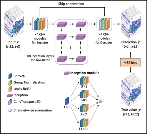
As DL-QPN can be perceived as a video prediction task, state-of-the-art video prediction models can be crucial to improving its performance. In this context, we propose DL-QPN models based on the simpler yet better video prediction (SimVP) suggested by Gao et al. (2022). SimVP uses only convolutional layers to learn both spatial and temporal features effectively, which is a notable advantage. In addition to an encoder – decoder structure similar to the structure of U-Net, SimVP has a powerful translator network between the encoder and decoder. By incorporating multiple inception modules with various kernel sizes, the translator significantly contributes to the transition of prediction between frames, which is a characteristic of RNNs.

The main goal of this study was to investigate the possibility of improving the forecasting skill of QPN using SimVP. First, we evaluated the models over the entire summer and early autumn (i.e. June – September) to test the overall performance. Next, three cases with different precipitation backgrounds were analyzed quantitatively and qualitatively. Finally, we conducted a comparison of model complexity to assess performance and efficiency together and investigate whether increased complexity results in improved performance.

2. Data and experimental design

2.1. Radar data over the Korean Peninsula

Ground weather radar data provided by the Korea Meteorological Administration (KMA) were used in this study. We used constant altitude plan position indicator (CAPPI) data, which represent the reflectivity at an altitude of 1.5 km (Figure 1a). The KMA provides composited CAPPI data from 11 radar sources with a spatial resolution of 1 km every 10 min. The radar reflectivity was converted to the precipitation rate (Figure 1b) based on the Z – R relationship (Marshall and Palmer 1948) and coefficients provided by the KMA (Equation 1(1) $Z=1.48R^{1.59}$(1) ):

Figure 1. Examples of data used in this study acquired at 09:50 KST on August 8, 2022. (a) Radar reflectivity, (b) radar precipitation intensity, and (c) AWS ground precipitation measurements. Gray area in (a) and (b) is the blank pixel area of radar coverage. Black rectangles in (a) and (b) indicate the area cropped to exclude blank pixels for model training. The entire area was used at the inference phase. Black triangles in (c) mark the AWS where no precipitation was measured.

(1) $Z=1.48R^{1.59}$(1)

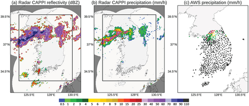
where Z is the radar reflectivity (mm⁶m⁻³) and R is the precipitation intensity (mm/h). As the original data contained blank pixels outside the radar coverage, we used only the data between 124.36 E and 130.42 E longitude and 33.64 N and 39.70 N latitude (black rectangles in Figure 1a,b) in the model training phase. The cropped radar area covered the entire mainland, the neighboring sea of South Korea, and some parts of North Korea. To evaluate the models, precipitation events during the latest summer and early autumn and all CAPPI data for June, July, August, and September (JJAS) in 2022 were used as the test dataset. CAPPI data of JJAS during 2019–2021 were used for training and validation.

2.2. Ground measurement data

We also evaluated model results using ground measurement data from automatic weather stations (AWS) provided by the KMA. The AWS measure wind speed and direction, temperature, humidity, surface pressure, and precipitation every minute. As the precipitation gauge in the AWS provides in situ surface precipitation, comparisons with AWS data can demonstrate model reliability and robustness. The total number of stations used in this study was 642 (Figure 1c).

2.3. Data split and evaluation cases

The CAPPI dataset was divided into training, validation, and testing datasets (Figure 2). During 2019–2021, radar data between the 1^st and 25^th of each month from June to September were used to train the DL-QPL models. The remaining data from the 26^th to the end of each month were used for internal validation of the model performance by optimizing their hyperparameters. The entire explicitly separated test dataset for June – September 2022 was only used to evaluate the final performance of the models. The evaluation of predicted precipitation relies heavily on the characteristics of the precipitation, such as the precipitation area, speed of shift, and intensity distribution. Because of the overlap between the precipitation in successive time steps, the probability of obtaining a higher skill score increases as the precipitation over the target area increases. To examine various conditions, four cases with different durations and types of precipitation were evaluated in detail (Table 1). With t-m and t+n representing the past m minutes of input data and n minutes of lead time, respectively, the radar sequence from t-110 to t-0 was used as the input sequence and that between t + 10 and t + 120 was employed as the target data.

Figure 2. Training (Train), validation (Val), and test data split scheme. Test data were totally separated as unseen from the model training and validation phases.

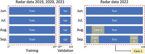
Table 1. Experimental design of the four test cases. The ratio represents the average pixel ratio over the given threshold for each scene.

Test	Period (2022)	Features	Ratio > 1 mm/h (%)	Ratio > 5 mm/h (%)	Ratio > 10 mm/h (%)
Case 1	Jun–Sep	Korean summer and early autumn	11.8	3.80	1.15
Case 2	Aug 7–11	Heavy rainfall	10.2	3.49	1.5
Case 3	00:00 Sep 05–12:00 Sep 06	Typhoon Hinnamnor	39.1	10.1	2.4
Case 4	20:00 Sep 22–16:10 Sep 23	Narrow convection	3.2	1.19	0.6

As performance evaluation depends highly on the period and pattern of rainfall events, both long-term and case-level validations are essential for measuring model performance. Case 1 covers all radar scenes through JJAS of 2022. The overall performance of the proposed model was evaluated based on case 1. Case 2 represents a historic heavy rainfall in South Korea that caused severe socioeconomic damage. Because of the strongly developed stationary front (in Korean, jangma) that remains in the middle of the Korean Peninsula, 578.5 mm of precipitation fell in Seoul, the capital city of South Korea, within four days, and the daily cumulative precipitation recorded reached a maximum of 381.5 mm on 8 August 2022. In this case, a large quantity of water vapor continuously flowed into a narrow area from the west as an atmospheric river formed due to high pressure in the northern Pacific Ocean and the northern part of the Korean Peninsula. Case 3 is the precipitation event induced by typhoon Hinnamnor, which developed on 27 August 2022. It was the first super typhoon of 2022 in the western North Pacific region. After weakening due to concentric eyewall cycles, it re-intensified as a super typhoon before approaching Okinawa, Japan, and then progressed to South Korea, where it produced more than 540 mm of precipitation, caused 13 deaths, and resulted in socioeconomic losses exceeding 1 billion USD. Finally, case 4 represents very narrow local convection that moved rapidly from west to east. The precipitable cloud was formed due to large quantities of warm water vapor brought by typhoon Talas from the Western Pacific to encountering cold air from a continental high pressure region located in the north (or continental Eurasia). Strong cumulonimbus clouds developed in a line from south to north, and the clouds moved rapidly from west to east while releasing heavy downpours of rain. This case can be used to measure model performance, especially for the rainfall shift and its phase change.

3. Methodology

3.1. Proposed SimVP-based model

Similar to other encoder – decoder models, such as U-Net, SimVP consists of an encoder, a translator, and a decoder with only CNN modules (Figure 4a and Table 2). The expected roles of the three components are as follows: the encoder is used for extracting spatial features, the translator is for learning spatiotemporal change over time, and the decoder is for integrating spatiotemporal information (Gao et al. 2022). The unique feature of SimVP is its translator, which employs N inception modules to learn temporal movements. By adopting the inception module (Szegedy et al. 2015), a translator can employ multiple sizes of convolutional kernels and their corresponding receptive fields. This feature is expected to significantly enhance the robustness of spatial modeling for input feature size. As spatial changes in QPN can vary at each time step, the ability to address various receptive areas can indirectly contribute to the coverage of various temporal data. The mean squared error (MSE) was used as a loss function. For model fitting, we used the Adaptive Momentum (Adam) optimizer (Kingma and Ba 2014) with a learning rate of 0.001 and 100 iterations. The Adam optimizer has been adopted widely as a representative optimizer in geoscientific modeling because of its fast and stable optimization properties (Lee et al. 2021; He et al. 2022; Franch et al. 2020; Gibson et al. 2021). As most of the dataset contained no precipitation, we set the batch size to 1 and skipped the training process when the ratio of precipitation pixels over 5 mm/h was less than 1% of each batch to avoid being optimized with zero-filled data. Hyperparameters, including optimizer, loss function, number of iterations, batch size, and blank data filtering conditions, were also adopted for all DL-QPN models used in this study in cases of no explicit description.

Table 2. Models used in this study. S-PROG stands for spectral prognosis suggested by (Seed 2003).

Model	Encoder	Translator	Decoder	GAN discriminator	Non-DL module
pySTEPS (Pulkkinen et al. 2019)	-	-	-	-	S-PROG STEPS
ConvLSTM (Shi et al. 2015)	ConvLSTM	-	ConvLSTM	-	-
U-Net (Ayzel, Scheffer, and Heistermann 2020)	CNN	CNN	CNN	-	-
Rad-cGAN (Choi and Kim 2022)	CNN	CNN	CNN	Patch GAN	-
PhyDNet (Guen and Thome 2020)	CNN	ConvLSTM, PhyCell	CNN	-	-
SimVP (Gao et al. 2022)	CNN	CNN Inception	CNN	-	-

Generally, a more complex model can be expected to have better modeling capacity. The original SimVP model has 4 layers for each encoder and decoder and 8 layers in the translator with a set of different kernel sizes of 3 × 3, 5 × 5, 7 × 7, and 11 × 11 (Figure 3). To test whether higher complexity produces better results, we doubled the number of encoder and decoder layers from 4 to 8 and quadrupled the number of inception layers from 8 to 32 with additional 15 × 15 and 21 × 21 kernels, which can be expected to count a larger area. However, the deeper SimVP model did not produce improvement in the validation metrics. Therefore, after several tests for optimal model structure, the original SimVP structure was adopted. A comparison and discussion of model complexity is included in Section 4.3.

Figure 3. Model structure for the proposed nowcasting model utilizing simpler yet better video prediction.

3.2. Comparison models

3.2.1. Python short-term ensemble prediction system (pySTEPS)

The pySTEPS (Pulkkinen et al. 2019) is an open-source Python framework for short-term ensemble prediction (https://pysteps.github.io) based on spectral prognosis (Seed 2003) and STEPS (Bowler, Pierce, and Seed 2006). It calculates the motion field from given radar data and conducts an extrapolation to generate future sequences. Post-processing includes statistical property matching between prediction results and the latest input. This can directly contribute to preventing the underestimation problem of DL-QPN models (Ravuri et al. 2021; Han et al. 2022). In this study, the motion field was obtained using the Lucas – Kanade optical flow method implemented in pySTEPS. The radar sequence from t-110 to t-0 was used to calculate a motion vector. Based on the motion vector, the future sequence from t + 10 to t + 120 was predicted.

3.2.2. ConvLSTM

In recent years, ConvLSTM has emerged as one of the most representative baseline models for spatiotemporal video prediction (Lin et al. 2020; Wang et al. 2018; Xiang et al. 2020). By incorporating a convolutional process into the LSTM module, ConvLSTM can handle spatial and temporal information (Shi et al. 2015). Several studies that adopted ConvLSTM and its successors in DL-QPN have reported their superiority over other baseline models (Shi et al. 2015, 2017; Franch et al. 2020; Ravuri et al. 2021; Xiong et al. 2021; Cuomo and Chandrasekar 2021; Jeong et al. 2021). To build a successful rainfall forecasting model, we used the seq2seq architecture suggested by Sutskever, Vinyals, and Le (2014). Seq2seq has been used widely for models utilizing time series data and natural language processes and can be considered a robust baseline forecasting model (Shengdong et al. 2020; Masood et al. 2022; Sutskever, Vinyals, and Le 2014). Seq2seq converts inputs to outputs using an LSTM-based encoder – decoder structure. As the original seq2seq model was not designed to reflect spatial information, its LSTM module was replaced with ConvLSTM for the spatiotemporal modeling of rainfall. Four ConvLSTM layers were used for each encoder and decoder. The size of the convolutional kernel was 3 × 3, and the numbers of kernels for each ConvLSTM layer were 32, 64, 64, and 32, respectively. A 3D convolutional layer with a linear activation function was used at the last output layer.

3.2.3. U-Net

U-Net (Ronneberger, Fischer, and Brox 2015) has been used widely in DL-QPN because of its robust ability to model not only segmentation but also the regression of future frames. Several studies have reported that U-Net achieved competitive performance in DL-QPN compared to the case without the RNN module (Agrawal et al. 2019; Ayzel, Scheffer, and Heistermann 2020; Trebing, Staǹczyk, and Mehrkanoon 2021). For comparison, in this study, we used RainNet v1.0, which is available with open-source codes (Ayzel, Scheffer, and Heistermann 2020). The original RainNet adopted a recursive prediction design, whose input sequence was four radar scenes for t-15, t-10, t-5, and t-0, to predict the next time step, t + 5. To predict t + 10 precipitation, the input sequence was updated with t-10, t-5, t-0, and t + 5. This recursive prediction approach is intuitive and may perform well in the near future within a few time steps. However, the prediction error is likely to accumulate as the lead time increases (Ayzel, Scheffer, and Heistermann 2020). We compared recursive and multiple-prediction designs using the RainNet structure (not shown here) and found that multiple predictions yielded significantly better performance with longer lead times. Hence, we adopted a multiple-prediction design for comparison with the proposed model. Based on RainNet, we designed U-Net to have four symmetric encoders and decoders, with 64, 128, 256, and 512 convolutional filters of 3 × 3 size, respectively.

3.2.4. Rad-cGAN

Choi and Kim (2022) proposed and tested a radar-based DL-QPN model with cGAN, namely Rad-cGAN, over the Korean Peninsula. We selected Rad-cGAN over the study area as a comparative model to examine the ability of cGAN because it uses the recent trend. The model architecture is based on the image-to-image translation model Pix2Pix, which consists of U-Net as the generator and PatchGAN as the discriminator (Isola et al. 2017). The original Rad-cGAN uses a recursive prediction approach with four past input frames to predict the subsequent frame. However, Rad-cGAN suffered from significant underestimation with longer lead time, resulting in a critical score index (CSI) of nearly zero when a 1 mm/h threshold was applied. In our pilot test between multistep and recursive prediction approaches, recursive prediction suffered from cumulative errors and lost its signal faster than did the multiple-prediction. Hence, as in other models, 12 radar inputs were used to generate 12 future sequences. The model structure of Rad-cGAN was the same as the original except for the input and output sequence length. Rad-cGAN was optimized with the Adam optimizer and binary cross-entropy function, as per Choi and Kim (2022). To optimize the GAN model fully, Rad-cGAN was trained with 200 iterations, which is twice the number for other DL-QPN models.

3.2.5. PhyDNet

PhyDNet integrates statistical (DL) and physical approaches within a translator. By combining partial differential equations and ConvLSTM, PhyDNet aims to derive a synergy between DL and non-DL models (Guen and Thome 2020). PhyDNet decomposes the input latent space into physical dynamic and residual factors. Physical dynamic factors are processed in a physical cell (PhyCell) with a recurrent structure based on data assimilation. PhyCell learns known physical dynamics at a coarser level, whereas ConvLSTM captures unknown fine-grained factors, such as appearance, texture, and details. As PhyDNet is a hybrid of physical and statistical approaches, it was used as a reference model for comparison. The original PhyDNet consists of a single PhyCell layer with 7 × 7 kernel size and 49 hidden dimensions and three ConvLSTM layers with 3 × 3 kernels and 128, 128, and 64 convolutional filters (Guen and Thome 2020). We also doubled the number of each PhyCell and ConvLSTM layer to test whether there was any model enhancement attributable to greater complexity; however, there was no significant improvement in the validation results, as reported in Section 4.3. Hence, the original PhyDNet structure was used in this study.

3.3. Evaluation

Model evaluation was performed using both quantitative and qualitative approaches. General metrics used in the DL-QPN, such as Pearson correlation (R), root-mean-squared error (RMSE), mean bias, and CSI, were used for the quantitative evaluation:

(2) $R=\frac{{\sum }_i^N\left(y_i-{\bar{y}}_i\right)\left({\hat{y}}_i-{\overline{\stackrel{ˆ}{y}}}_i\right)}{\sqrt{{\sum }_i^N{\left(y_i-{\bar{y}}_i\right)}^2{\sum }_i^N{\left({\hat{y}}_i-{\overline{\stackrel{ˆ}{y}}}_i\right)}^2}}$(2)

(3) $RMSE=\sqrt{\frac{{\sum }_i^N{\left(y_i-{\hat{y}}_i\right)}^2}{N}}$(3)

(4) $meanbias=\frac{{\sum }_i^N\left(y_i-{\hat{y}}_i\right)}{N}$(4)

(5) $CSI=\frac{TP}{TP+FN+FP},where\text{break}\left\{\begin{array}{c}TP={\sum }_i^N\left(1,if{y}_i\ge \alpha and{\hat{y}}_i\ge \alpha ;0,otherwise\right)\\ FN={\sum }_i^N(1,if{y}_i\ge \alpha and{\hat{y}}_i<\alpha ;0,otherwise)\\ FP={\sum }_i^N(1,if{y}_i<\alpha and{\hat{y}}_i\ge \alpha ;0,otherwise)\end{array}\right.$(5)

where y and $\hat{y}$ denote the truth and prediction of the i^th pixel, respectively. TP, FN, and FP represent the sum of true positive, false negative, and false positive pixels with the given precipitation threshold $\alpha$, respectively. The range of CSI is from 0 to 1, and higher CSI indicates better model performance.

4. Results and discussion

4.1. Performance evaluation of all models for case 1

Figure 4a depicts the CSI with different lead times for the thresholds of 1, 5, and 10 mm/h in comparison with radar CAPPI. With a lead time of 10 min, all DL-based models, with the exception of Rad-cGAN, yielded similar CSI for all three thresholds. SimVP showed higher CSI than the other models with a threshold of 1 mm/h and with increasing lead time. As the CSI measures the correctness of an area match with a given threshold, this result implies that SimVP demonstrated improved performance compared to the other DL models for predicting overall precipitation. However, with the threshold of 5 mm/h, PhyDNet and SimVP yielded better performance than the other models. Although SimVP also demonstrated better performance for the 10 mm/h threshold, the performance gap became negligible when the lead time was approximately 120 min.

Figure 4. CSI performance from June to September 2022 in South Korea (case 1). Evaluation results with (a) radar CAPPI and (b) AWS in situ measurements.

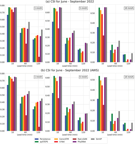
The comparison with AWS in situ measurements showed a similar CSI pattern of radar data (Figure 4b). Evaluation using in situ data is crucial for operational purposes. The SimVP model also outperformed the others in terms of CSI in validation with AWS data, implying that the proposed model can predict upcoming precipitation in the area where the AWS is located with higher performance, as measured by CSI, than the others.

Table 3 shows the overall performance of the models in terms of R, RMSE, CSI, and mean bias. To separate the overall rainfall (>1 mm/h) from that with stronger intensities, we separated the CSI and bias scores using thresholds of 1, 5, and 10 mm/h. Each metric followed by a number (e.g. RMSE1, CSI5, or Bias10) indicates that the metric was evaluated with the threshold indicated by the corresponding number. As determined by the RMSE with the 1 mm/h threshold (RMSE1), SimVP yielded slightly higher errors than other DL-based models for lead times of 10, 60, and 120 min. However, with the higher thresholds of 5 and 10 mm/h, the gap narrowed. The R of all models was approximately 0.8, demonstrating a high correlation despite a significant decrease with the increase in lead time. In addition to SimVP, PhyDNet also yielded higher correlations than other models for lead times of 60 and 120 min. The magnitude of the mean bias can indicate how the average intensity increases or decreases compared to that of radar data (Zhang et al. 2021). Except for pySTEPS, all DL-based models showed a significantly increasing magnitude of negative mean bias as the threshold and lead time increased. SimVP showed the lowest magnitude of Bias10 among the DL models, indicating a lesser underestimation problem than other models. However, the suggested SimVP model still suffered from the common underestimation problem of the DL-QPN, which has been reported in many studies (Ayzel, Scheffer, and Heistermann 2020; Choi and Kim 2022).

Table 3. Evaluation with radar data for case 1. Numbers after each metric indicate the thresholds of 1, 5, and 10 mm/h. The precipitation pixels lower than the threshold in both radar and predicted values were not counted in the performance calculation. The best performance for each metric is indicated in bold font.

Lead time	R	RMSE1	RMSE5	RMSE10	CSI1	CSI5	CSI10	Bias1	Bias5	Bias10
10 min
Persistence	0.56	7.41	11.47	15.96	0.67	0.49	0.36	0.00	−0.01	−0.02
pySTEPS	0.82	4.76	7.46	10.46	0.78	0.65	0.56	−0.11	−0.28	−0.57
ConvLSTM	0.83	4.47	7.22	10.33	0.77	0.65	0.53	−0.46	−1.47	−3.10
U-Net	0.79	4.84	7.64	10.87	0.74	0.61	0.49	−0.23	−0.95	−2.54
Rad-cGAN	0.81	6.38	10.47	15.11	0.71	0.41	0.27	−3.03	−6.71	−11.17
PhyDNet	0.84	4.25	6.78	9.57	0.77	0.66	0.56	−0.15	−0.65	−1.59
SimVP	0.84	4.35	6.82	9.66	0.77	0.66	0.56	0.16	−0.10	−0.96
60 min
Persistence	0.13	10.04	15.37	21.40	0.41	0.22	0.12	0.05	0.14	0.28
pySTEPS	0.25	9.45	14.51	20.12	0.48	0.29	0.18	−0.45	−0.86	−1.37
ConvLSTM	0.31	6.77	11.98	18.82	0.48	0.26	0.09	−0.94	−4.57	−12.15
U-Net	0.35	6.43	11.41	17.72	0.48	0.30	0.13	−0.28	−3.11	−9.38
Rad-cGAN	0.16	9.58	16.01	23.04	0.26	0.02	0.00	−5.10	−11.69	−19.04
PhyDNet	0.43	6.45	11.37	17.49	0.47	0.35	0.16	−0.76	−3.69	−9.93
SimVP	0.43	6.88	11.29	16.54	0.57	0.38	0.22	−0.51	−2.36	−6.09
120 min
Persistence	0.02	10.33	15.93	22.36	0.32	0.15	0.08	0.20	0.50	0.91
pySTEPS	0.03	10.37	15.94	22.20	0.34	0.16	0.08	−0.71	−1.29	−1.88
ConvLSTM	0.12	6.54	13.34	21.14	0.37	0.11	0.01	−0.93	−7.06	−16.52
U-Net	0.14	6.57	12.95	20.37	0.38	0.13	0.03	−0.85	−5.88	−14.29
Rad-cGAN	−0.01	9.84	16.45	23.55	0.08	0.00	0.00	−5.59	−12.45	−19.84
PhyDNet	0.22	6.45	11.77	20.16	0.37	0.23	0.03	−0.61	−3.85	−14.85
SimVP	0.20	7.36	12.66	19.02	0.46	0.23	0.09	−1.16	−4.44	−10.32

4.2. Evaluation over precipitation events

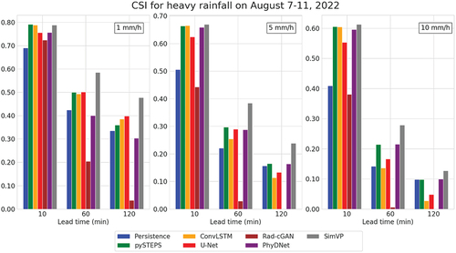
Figures 5–7 show the CSI scores with lead times of 10, 60, and 120 min for cases 2–4, respectively. As shown in Figure 5, for case 2, the suggested SimVP outperformed the other models for all three thresholds with lead times of 60 and 120 min. As the average rainfall intensity was higher than that in case 1 (all precipitation events in June – September 2022), all models showed relatively better performances in general compared to that in case 1 because of the long-lasting heavy rainfall event. ConvLSTM and U-Net yielded a higher CSI1 than PhyDNet in case 2. As CSI1 is directly related to the match of all precipitation areas, PhyDNet failed to model the area of precipitation successfully in this case.

Figure 5. Performance in terms of CSI for the heavy rainfall event of August 7–11, 2022, KST in South Korea (case 2).

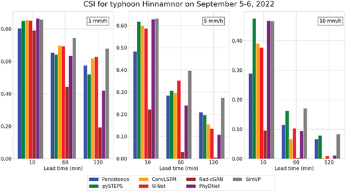
The CSI scores for case 3 are shown in Figure 6. During typhoon Hinnamnor, a large portion of the radar coverage area contained precipitation pixels. When the change in precipitation areas was relatively small compared to the total precipitation area, the probability of achieving inflated performance without meaningful prediction increased. For instance, even the persistence scheme achieved a score that was relatively high or comparable to those of the DL models. Hence, performance analysis should be conducted carefully with consideration of the characteristics of each precipitation event, such as the coverage ratio, intensity distribution, duration, and shift and development speed. Compared with the vast precipitation area with a threshold of 1 mm/h, the precipitation area with a threshold of 10 mm/h rapidly decreased in case 3, as shown in Table 1. This could result in a large CSI difference between the thresholds of 1 mm/h and 10 mm/h (Figure 6). Most models showed similar prediction performance at the lead time of 10 min. With lead times of 60 and 120 min, SimVP showed the best performance (Figure 6).

Figure 6. CSI performance for typhoon Hinnamnor on September 5–6, 2022, in South Korea (case 3).

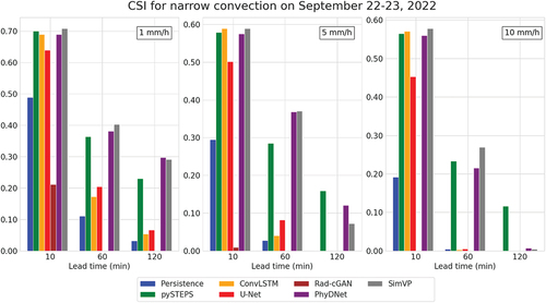
The results for the narrow convection event with a rapid shift are shown in Figure 7. As shown in the figure, the overall performances of all models were significantly lower than those observed in previous cases, especially case 3. There is a much lower probability of obtaining a high CSI by chance because of the fast-moving precipitation cell. PySTEPS showed the best performance in CSI10 with a 120 min lead time, whereas all the other models showed nearly zero performance.

Figure 7. CSI performance for the narrow convection during September 22–23, 2022, in South Korea (case 4).

Figures 8–10 show the prediction maps for cases 2–4, respectively. Figure 8 shows the prediction map for the extreme rainfall event starting at 11:40 on 8 August 2022, with lead times from 10 to 120 min. In Figure 8, PhyDNet shows a different developing shape than the other models. In terms of precipitation intensity, all DL models showed a decreasing trend, unlike pySTEPS. When the shape and intensity did not change significantly until the target lead time, pySTEPS appeared to provide better performance than other models, especially in terms of precipitation intensity. In Figure 9, for case 3, blurry patterns of DL-QPN can be observed clearly over the vast area as the lead time increases. Even though SimVP showed the highest CSI1 with lead times longer than 60 min, the smoothing effect should be improved further to convey detailed information.

Figure 8. Prediction maps of the severe rainfall event in South Korea from 9:50–11:40 KST on August 8, 2022 (case 2). Each subfigure is a forecast with a lead time in minutes. The lead time t+10 min is 09:50, and the lead time t+120 min is 11:40. The location where the precipitation pixels vanished in the 120 min lead time is shown by a black dotted circle in radar t+10.

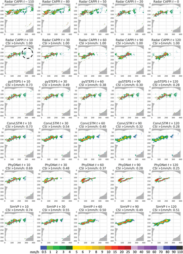
In Figure 10, no precipitation remains in the radar CAPPI map 120 min ahead when compared to that at the 10 min lead time (black dashed rectangle in radar CAPPI t + 120). ConvLSTM failed to simulate horizontal movement, and the precipitation intensities decreased without the advantage of hovering precipitation. The results of pySTEPS showed almost linear movement from west to east; however, the CSI performance did not increase by chance because of the narrow precipitation area. Among the DL models, PhyDNet and SimVP clearly showed changes in displacement and shape. Both displacement movements and shape shifts occurred; however, neither of these successfully mimicked the actual distribution of precipitation areas and intensities. They predicted development of new, although weak, precipitation with a larger precipitation area over time (black dashed circle in Figure 10).

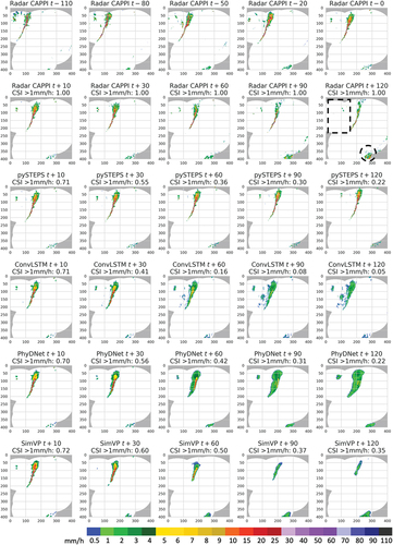
Figure 9. Prediction maps for typhoon Hinnamnor in South Korea from 23:50 KST September 5 to 01:40 KST September 6, 2022 (case 3). Each subfigure is a forecast with a lead time in minutes. The lead time t+10 min is 23:50 September 5, and the lead time t+120 min is 01:40 September 6, 2022.

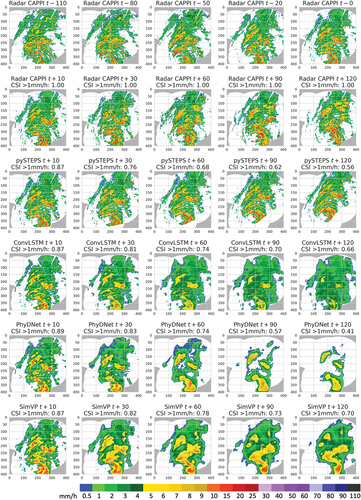
Figure 10. Prediction maps for the narrow convection in South Korea during 10:20–12:10 KST on September 23, 2022 (case 4). Each subfigure is a forecast with a lead time in minutes. The lead time t+10 min is 10:20, and the lead time t+120 min is 12:10. The location where the precipitation pixels vanished in the 120 min time is shown by a black dotted rectangle, and a newly developing area is indicated with a black dotted circle in radar t+120.

4.3. Model complexity

The importance of complexity of a DL model lies in its implementation, accessibility to various computational resources, and reduced optimization time through multiple trials. We evaluated the complexity of the DL models (Table 4) using the PyTorch FLOPs counter library (https://github.com/sovrasov/flops-counter.pytorch). GPU memory usage for all models ranged from approximately 2.7 to 4.6 GB for a single batch, with dimensions of 12 × 1 × 304 × 304 (time, channel, height, and width, respectively) for each input and output sequence during the training phase. Floating operations (FLOPs) account for the total operation counts utilizing the weights, and the number of parameters (Params) represents the total weights in the model. In general, a more complex model has larger FLOPs and Params, resulting in larger model size and higher training time. Among the DL-QPN models, ConvLSTM exhibited significantly lower Params and model size (Table 4). The small Params in RNNs can be attributed to their inherent property of weight sharing across time steps, potentially leading to a more compact model (Goodfellow, Bengio, and Courville 2016). Despite having lower FLOPs and Params than other models, ConvLSTM did not have a significantly lower training time (383 s), even exceeding that of U-Net (297 s). The sequential nature of RNN models makes parallelization difficult (Hochreiter and Schmidhuber 1997; Cho et al. 2014), which may result in longer training times for relatively simple models. The extended training time of PhyDNet could be partly due to its integration of ConvLSTM. Conversely, the CNN-based models (e.g. U-Net, Rad-cGAN, and SimVP) demonstrated relatively fast training times, considering their FLOPs and Params. The saved model size correlates almost linearly with Params, with each parameter occupying approximately 12 bytes in the saved files.

Table 4. Complexity comparison of DL-QPN models for radar sequence data. The memory, FLOPs, and Params listed are for a single batch sample. Training time represents the duration of a single epoch using an NVIDIA RTX 3090Ti GPU. The input and output radar sequences have dimensions of 12 × 1 × 304 × 304, corresponding to time step, channel, width, and height, respectively. Val CSI5 refers to the validation CSI5 at the final epoch for each model. In this context, the + symbol in PhyDNet+ and SimVP+ indicates a modified, more complex structure than the original.

Model	Memory	FLOPs	Params	Saved model size	Training time per epoch	Val CSI5 (t+10)	Val CSI5 (t+120)
ConvLSTM	3884 MB	89.82 G	79.88 K	981.0 KB	383 s	0.67	0.15
U-Net	2708 MB	158.46 G	31.39 M	376.7 MB	297 s	0.54	0.23
Rad-cGAN	4330 MB	613.4 G	15.69 M	188.4 MB	454 s	0.46	0.00
PhyDNet	4596 MB	1673.2 G	3.09 M	37.2 MB	1967 s	0.66	0.24
PhyDNet+	5658 MB	2705.8 G	5.09 M	58.4 MB	2785 s	0.63	0.17
SimVP	4268 MB	183.1 G	13.98 M	168.1 MB	635 s	0.67	0.23
SimVP+	9804 MB	529.2 G	239.3 M	2.7 GB	2380 s	0.58	0.20

The model structure optimization and hyperparameter tuning were performed by monitoring the CSI5 of the very first (t+10) and last (t+120) time steps of the validation dataset, taking into account the moderate precipitation intensity at both ends of the forecast. To ensure that the test data remained completely unseen, hyperparameter optimization was carried out using only a separate validation dataset. Table 4 summarizes the complexity and validation performance of more complex variants of the two best DL models (PhyDNet and SimVP), indicated as PhyDNet+ and SimVP+. As mentioned in Sections 3.1 and 3.2, these models did not show improved validation performance despite having a deeper structure. Generally, increased complexity may provide a higher learning capacity, but it does not always lead to better performance. This implies that enhancing model performance merely by augmenting model complexity within a specific dataset and DL model structure can be difficult. Consequently, alternative approaches, such as utilizing different loss functions or investigating innovative model designs, should be explored in future studies to boost model performance further.

4.4. Novelty and limitations

This study proposes precipitation nowcasting models for up to 120 min using SimVP DL. The proposed model, powered by state-of-the-art architecture, showed improved performance compared to the results of previous studies and can serve as a new baseline model for DL-QPN. With the relatively simple structure of the original open-source code proposed by Gao et al. (2022), reproduction of the models used in this study should be much easier than that of more complex previous models without a shared code. Although there have been many DL-QPN-based studies, most of these conducted visual interpretation over scenes with large rainfall ratios, often inflating model accuracy (Ayzel, Scheffer, and Heistermann 2020; Choi and Kim 2022; Liu, Lei, and Chen 2022; Zhang et al. 2022; Yang et al. 2022). To demonstrate both the success and limitations of the proposed SimVP-based model over different precipitation events, we analyzed three individual cases along with a long-term evaluation from June to September 2022. A comparison of model complexity was also carried out to consider operational applications across different study areas and environments of DL-QPN models. By analyzing these various cases, which demonstrate both the potential and limitations of the proposed SimVP-based model, we believe that this study supports a new baseline for DL-QPN.

Despite the novelty and contribution of this study, it has some limitations that require attention in future studies. Most importantly, this study did not compare the suggested model with operational forecasting models such as NWP. As our target was radar-based forecasting, it was difficult to compare other prediction results directly because of the different data sources. Another limitation is that the suggested model suffered from underestimation and blurry effects, similar to the models used in previous studies. To avoid the underestimation problem encountered at larger lead times, an explicit module for learning the tendency of the intensity distribution will be investigated in the future.

5. Conclusions

This study suggests a SimVP-based model for precipitation nowcasting. Compared with other representative models (i.e. ConvLSTM and U-Net) and recent models utilizing GAN and physical modules (i.e. Rad-cGAN and PhyDNet), the suggested SimVP model showed better performance in terms of CSI score and visual interpretation. An evaluation using precipitation events for the entire summer and early autumn of 2022 indicated that SimVP yielded higher R and CSI and a lower magnitude of negative bias during heavy rainfall events. The comparison with the AWS in situ measurements over JJAS 2022 demonstrated the robustness and reliability of the proposed SimVP model. To consider various precipitation conditions, the performances of the models were analyzed according to three cases: heavy rainfall, typhoon, and narrow convection. We found that the performance and mapping results varied case-wise. Consequently, the performance of the DL-QPN should be evaluated carefully, with a particular focus on poor performance. The suggested SimVP model showed the best performance in terms of CSI in the heavy rainfall and typhoon cases and comparable performance to PhyDNet in the narrow convection case. The model complexity analysis revealed that the proposed SimVP exhibited longer training time (about twice as long) than ConvLSTM and U-Net, but it had significantly lower FLOPs and training time than PhyDNet, which showed the best performance among the comparison models. Overall, the proposed model with improved prediction performance (i.e. improved precipitation nowcasting), can be used to ensure socioeconomic damage reduction or prevention caused by intense precipitation events.

Acknowledgments

This research was supported by the MSIT (Ministry of Science and ICT), Korea, under the ITRC (Information Technology Research Center) support program(IITP-2023-2018-0-01424) supervised by the IITP(Institute for Information & communications Technology Promotion), and by “Development of risk managing technology tackling ocean and fisheries crisis around Korean Peninsula by Kuroshio Current” of the Korea Institute of Marine Science and Technology Promotion (KIMST), funded by the Ministry of Oceans and Fisheries (RS-2023-00256330).

Disclosure statement

No potential conflict of interest was reported by the authors.

Data availability statement

The radar and AWS raw data are available at the KMA data portal, as follows.

Source codes for each model can be obtained in our GitHub repository.

- Radar data: https://data.kma.go.kr/data/rmt/rmtList.do?code=11&pgmNo=62

- AWS in situ data: https://data.kma.go.kr/data/grnd/selectAwsRltmList.do?pgmNo=56

- GitHub repository: https://github.com/daehyeon-han/qpn-simvp

References

- Agrawal, S., L. Barrington, C. Bromberg, J. Burge, C. Gazen, and J. Hickey. 2019. “Machine Learning for Precipitation Nowcasting from Radar Images.” arXiv preprint arXiv:1912.12132. doi:10.48550/arXiv.1912.12132.
- Ayzel, G., T. Scheffer, and M. Heistermann. 2020. “RainNet V1. 0: A Convolutional Neural Network for Radar-Based Precipitation Nowcasting.” Geoscientific Model Development 13 (6): 2631–19. doi:10.5194/gmd-13-2631-2020.
- Bechini, R., and V. Chandrasekar. 2017. “An Enhanced Optical Flow Technique for Radar Nowcasting of Precipitation and Winds.” Journal of Atmospheric and Oceanic Technology 34 (12): 2637–2658. doi:10.1175/JTECH-D-17-0110.1.
- Bowler, N. E., C. E. Pierce, and A. Seed. 2004. “Development of a Precipitation Nowcasting Algorithm Based Upon Optical Flow Techniques.” Journal of Hydrology 288 (1–2): 74–91. doi:10.1016/j.jhydrol.2003.11.011.
- Bowler, N. E., C. E. Pierce, and A. W. Seed. 2006. “STEPS: A Probabilistic Precipitation Forecasting Scheme Which Merges an Extrapolation Nowcast with Downscaled NWP.” Quarterly Journal of the Royal Meteorological Society: A Journal of the Atmospheric Sciences, Applied Meteorology and Physical Oceanography 132 (620): 2127–2155. doi:10.1256/qj.04.100.
- Chen, L., Y. Cao, M. Leiming, and J. Zhang. 2020. “A Deep Learning‐based Methodology for Precipitation Nowcasting with Radar.” Earth and Space Science 7 (2): e2019EA000812. doi:10.1029/2019EA000812.
- Choi, S., and Y. Kim. 2022. “Rad- Cgan V1. 0: Radar-Based Precipitation Nowcasting Model with Conditional Generative Adversarial Networks for Multiple Dam Domains.” Geoscientific Model Development 15 (15): 5967–5985. doi:10.5194/gmd-15-5967-2022.
- Cho, K., B. Van Merriënboer, C. Gulcehre, D. Bahdanau, F. Bougares, H. Schwenk, and Y. Bengio. 2014. “Learning phrase representations using RNN encoder-decoder for statistical machine translation.” arXiv preprint arXiv:1406.1078. doi: 10.3115/v1/D14-1179.
- Cuomo, J., and V. Chandrasekar. 2021. “Use of Deep Learning for Weather Radar Nowcasting.” Journal of Atmospheric and Oceanic Technology 38 (9): 1641–1656. doi:10.1175/JTECH-D-21-0012.1.
- Foresti, L., I. V. Sideris, D. Nerini, L. Beusch, and U. Germann. 2019. “Using a 10-Year Radar Archive for Nowcasting Precipitation Growth and Decay: A Probabilistic Machine Learning Approach.” Weather and Forecasting 34 (5): 1547–1569. doi:10.1175/WAF-D-18-0206.1.
- Franch, G., D. Nerini, M. Pendesini, L. Coviello, G. Jurman, and C. Furlanello. 2020. “Precipitation Nowcasting with Orographic Enhanced Stacked Generalization: Improving Deep Learning Predictions on Extreme Events.” Atmosphere 11 (3): 267. doi:10.3390/atmos11030267.
- Gao, Z., C. Tan, W. Lirong, and S. Z. Li. 2022. “SimVp: Simpler Yet Better Video Prediction.” Paper presented at the Proceedings of the IEEE/CVF Conference on Computer Vision and Pattern Recognition, New Orleans, June 19–24.
- Germann, U., and I. Zawadzki. 2002. “Scale-Dependence of the Predictability of Precipitation from Continental Radar Images. Part I: Description of the Methodology.” Monthly Weather Review 130 (12): 2859–2873. doi:10.1175/1520-049320021302859:SDOTPO2.0.CO;2.
- Gibson, P. B., W. E. Chapman, A. Altinok, L. Delle Monache, M. J. DeFlorio, and D. E. Waliser. 2021. “Training Machine Learning Models on Climate Model Output Yields Skillful Interpretable Seasonal Precipitation Forecasts.” Communications Earth & Environment 2 (1): 1–13. doi:10.1038/s43247-021-00225-4.
- Goodfellow, I., Y. Bengio, and A. Courville. 2016. Deep Learning. Cambridge, Massachusetts: MIT press.
- Goodfellow, I. J., J. Pouget-Abadie, M. Mirza, X. Bing, D. Warde-Farley, S. Ozair, A. C. Courville, and Y. Bengio. 2014. Generative Adversarial Nets. Paper presented at the NIPS.
- Guen, V. L., and N. Thome. 2020. “Disentangling Physical Dynamics from Unknown Factors for Unsupervised Video Prediction.” Paper presented at the Proceedings of the IEEE/CVF Conference on Computer Vision and Pattern Recognition, Virtual, June 14–19.
- Haiden, T., A. Kann, C. Wittmann, G. Pistotnik, B. Bica, and C. Gruber. 2011. “The Integrated Nowcasting Through Comprehensive Analysis (INCA) System and Its Validation Over the Eastern Alpine Region.” Weather and Forecasting 26 (2): 166–183. doi:10.1175/2010WAF2222451.1.
- Ham, Y.G., J.H. Kim, and J.J. Luo. 2019. “Deep Learning for Multi-Year ENSO Forecasts.” Nature 573 (7775): 568–572. doi:10.1038/s41586-019-1559-7.
- Han, L., J. Zhang, H. Chen, W. Zhang, and S. Yao. 2022. “Toward the Predictability of a Radar-Based Nowcasting System for Different Precipitation Systems.” IEEE Geoscience and Remote Sensing Letters 19: 1–5. doi:10.1109/LGRS.2022.3185031.
- He, D., Q. Shi, X. Liu, Y. Zhong, G. Xia, and L. Zhang. 2022. “Generating Annual High Resolution Land Cover Products for 28 Metropolises in China Based on a Deep Super-Resolution Mapping Network Using Landsat Imagery.” GIScience & Remote Sensing 59 (1): 2036–2067. doi:10.1080/15481603.2022.2142727.
- Hochreiter, S., and J. Schmidhuber. 1997. “Long Short-Term Memory.” Neural Computation 9 (8): 1735–1780. doi:10.1162/neco.1997.9.8.1735.
- Imhoff, R. O., C. C. Brauer, A. Overeem, A. H. Weerts, and R. Uijlenhoet. 2020. “Spatial and Temporal Evaluation of Radar Rainfall Nowcasting Techniques on 1,533 Events.” Water Resources Research 56 (8): e2019WR026723. doi:10.1029/2019WR026723.
- Isola, P., J.Y. Zhu, T. Zhou, and A. A. Efros. 2017. “Image-To-Image Translation with Conditional Adversarial Networks.” Paper presented at the Proceedings of the IEEE conference on computer vision and pattern recognition, Hawaii, July 21–26.
- Jeong, C. H., W. Kim, W. Joo, D. Jang, and Y. Mun Yong. 2021. “Enhancing the Encoding-Forecasting Model for Precipitation Nowcasting by Putting High Emphasis on the Latest Data of the Time Step.” Atmosphere 12 (2): 261. doi:10.3390/atmos12020261.
- Jihoon, K., K. Lee, H. Hwang, O. Seok-Geun, S.W. Son, and K. Shin. 2022. “Effective Training Strategies for Deep-Learning-Based Precipitation Nowcasting and Estimation.” Computers & Geosciences 161: 105072. doi:10.1016/j.cageo.2022.105072.
- Kang, J., H. Wang, F. Yuan, Z. Wang, J. Huang, and T. Qiu. 2020. “Prediction of Precipitation Based on Recurrent Neural Networks in Jingdezhen, Jiangxi Province, China.” Atmosphere 11 (3): 246. doi:10.3390/atmos11030246.
- Kim, Y., and S. Hong. 2021. “Very Short-Term Rainfall Prediction Using Ground Radar Observations and Conditional Generative Adversarial Networks.” IEEE Transactions on Geoscience and Remote Sensing. doi: 10.1109/TGRS.2021.3108812.
- Kim, S., S. Hong, M. Joh, and S.K. Song. 2017. “Deeprain: Convlstm Network for Precipitation Prediction Using Multichannel Radar Data.” arXiv preprint arXiv:1711.02316.
- Kingma, D. P., and J. Ba 2014. “Adam: A method for stochastic optimization.” arXiv preprint arXiv:1412.6980. doi: 10.48550/arXiv.1412.6980.
- Kodali, N., J. Abernethy, J. Hays, and Z. Kira. 2017. “On Convergence and Stability of Gans.” arXiv preprint arXiv:1705.07215.
- Kumar, D., A. Singh, P. Samui, and R. Kumar Jha. 2019. “Forecasting Monthly Precipitation Using Sequential Modelling.” Hydrological Sciences Journal 64 (6): 690–700. doi:10.1080/02626667.2019.1595624.
- LeCun, Y., L. Bottou, Y. Bengio, and P. Haffner. 1998. “Gradient-Based Learning Applied to Document Recognition.” Proceedings of the IEEE 86 (11): 2278–2324. doi:10.1109/5.726791.
- Lee, J., M. Kim, J. Im, H. Han, and D. Han. 2021. “Pre-Trained Feature Aggregated Deep Learning-Based Monitoring of Overshooting Tops Using Multi-Spectral Channels of GeoKompsat-2A Advanced Meteorological Imagery.” GIScience & Remote Sensing 58 (7): 1052–1071. doi:10.1080/15481603.2021.1960075.
- Lin, Z., L. Maomao, Z. Zheng, Y. Cheng, and C. Yuan. 2020. “Self-Attention Convlstm for Spatiotemporal Prediction.” Paper presented at the Proceedings of the AAAI conference on artificial intelligence, February 7–12, New York.
- Liu, T., A. Abd-Elrahman, J. Morton, and V. L. Wilhelm. 2018. “Comparing Fully Convolutional Networks, Random Forest, Support Vector Machine, and Patch-Based Deep Convolutional Neural Networks for Object-Based Wetland Mapping Using Images from Small Unmanned Aircraft System.” GIScience & Remote Sensing 55 (2): 243–264. doi:10.1080/15481603.2018.1426091.
- Liu, J., X. Lei, and N. Chen. 2022. “A Spatiotemporal Deep Learning Model ST-LSTM-SA for Hourly Rainfall Forecasting Using Radar Echo Images.” Journal of Hydrology 127748: 127748. doi:10.1016/j.jhydrol.2022.127748.
- Marshall, J. S., and W. K. M. Palmer. 1948. “The Distribution of Raindrops with Size.” J. meteor. 5:165–166. doi: 10.1175/1520-04691948005<0165:TDORWS>2.0.CO;2.
- Masood, Z., R. Gantassi, Y. Choi, and Y. Choi. 2022. “A Multi-Step Time-Series Clustering-Based seq2seq Lstm Learning for a Single Household Electricity Load Forecasting.” Energies 15 (7): 2623. doi:10.3390/en15072623.
- Mirza, M., and S. Osindero. 2014. “Conditional Generative Adversarial Nets.” arXiv preprint arXiv:1411.1784.
- Park, E., J. Hyun-Woo, W.K. Lee, S. Lee, C. Song, H. Lee, S. Park, W. Kim, and T.H. Kim. 2022. “Development of Earth Observational Diagnostic Drought Prediction Model for Regional Error Calibration: A Case Study on Agricultural Drought in Kyrgyzstan.” GIScience & Remote Sensing 59 (1): 36–53. doi:10.1080/15481603.2021.2012370.
- Pulkkinen, S., D. Nerini, A. A. Pérez Hortal, C. Velasco-Forero, A. Seed, U. Germann, and L. Foresti. 2019. “Pysteps: An Open-Source Python Library for Probabilistic Precipitation Nowcasting (V1. 0).” Geoscientific Model Development 12 (10): 4185–4219. doi:10.5194/gmd-12-4185-2019.
- Ravuri, S., K. Lenc, M. Willson, D. Kangin, R. Lam, P. Mirowski, M. Fitzsimons, M. Athanassiadou, S. Kashem, and S. Madge. 2021. “Skilful Precipitation Nowcasting Using Deep Generative Models of Radar.” Nature 597 (7878): 672–677. doi:10.1038/s41586-021-03854-z.
- Ronneberger, O., P. Fischer, and T. Brox. 2015. “U-Net: Convolutional Networks for Biomedical Image Segmentation.” Paper presented at the International Conference on Medical image computing and computer-assisted intervention, Munich, October 5–9.
- Sadeghi, M., A. Akbari Asanjan, M. Faridzad, P. Nguyen, K. Hsu, S. Sorooshian, and D. Braithwaite. 2019. “PERSIANN-CNN: Precipitation Estimation from Remotely Sensed Information Using Artificial Neural Networks–Convolutional Neural Networks.” Journal of Hydrometeorology 20 (12): 2273–2289. doi:10.1175/JHM-D-19-0110.1.
- Seed, A. W. 2003. “A Dynamic and Spatial Scaling Approach to Advection Forecasting.” Journal of Applied Meteorology 42 (3): 381–388. doi:10.1175/1520-0450(2003)042<0381:ADASSA>2.0.CO;2.
- Shengdong, D., L. Tianrui, Y. Yang, and S.J. Horng. 2020. “Multivariate Time Series Forecasting via Attention-Based Encoder–Decoder Framework.” Neurocomputing 388: 269–279. doi:10.1016/j.neucom.2019.12.118.
- Shi, X., Z. Chen, H. Wang, D.Y. Yeung, W.K. Wong, and W.C. Woo. 2015. “Convolutional LSTM Network: A Machine Learning Approach for Precipitation Nowcasting.” Advances in Neural Information Processing Systems 28. doi:10.48550/arXiv.1506.04214.
- Shi, X., Z. Gao, L. Lausen, H. Wang, D.Y. Yeung, W.K. Wong, and W.C. Woo. 2017. “Deep Learning for Precipitation Nowcasting: A Benchmark and a New Model.” Advances in Neural Information Processing Systems 30. doi:10.48550/arXiv.1706.03458.
- Sideris, I. V., L. Foresti, D. Nerini, and U. Germann. 2020. “NowPrecip: Localized Precipitation Nowcasting in the Complex Terrain of Switzerland.” Quarterly Journal of the Royal Meteorological Society 146 (729): 1768–1800. doi:10.1002/qj.3766.
- Sutskever, I., O. Vinyals, and Q. V. Le. 2014. “Sequence to Sequence Learning with Neural Networks.“ Advances in Neural Information Processing Systems, Montreal, December 8–13. 27.
- Szegedy, C., W. Liu, Y. Jia, P. Sermanet, S. Reed, D. Anguelov, D. Erhan, V. Vanhoucke, and A. Rabinovich. 2015. “Going Deeper with Convolutions.” Paper presented at the Proceedings of the IEEE conference on computer vision and pattern recognition, Boston, June 7–12.
- Tao, C., Y. Meng, L. Junjie, B. Yang, H. Fengmin, L. Yuanxi, C. Cui, and W. Zhang. 2022. “MSNet: Multispectral Semantic Segmentation Network for Remote Sensing Images.” GIScience & Remote Sensing 59 (1): 1177–1198. doi:10.1080/15481603.2022.2101728.
- Trebing, K., T. Staǹczyk, and S. Mehrkanoon. 2021. “SmaAt-UNet: Precipitation Nowcasting Using a Small Attention-UNet Architecture.” Pattern Recognition Letters 145: 178–186. doi:10.1016/j.patrec.2021.01.036.
- Wang, Y., Z. Gao, M. Long, J. Wang, and S. Yu Philip. 2018. “Predrnn++: Towards a Resolution of the Deep-In-Time Dilemma in Spatiotemporal Predictive Learning.” Paper presented at the International Conference on Machine Learning, Stockholm, July 10–15.
- Xiang, X., Y. Tian, Y. Zhang, F. Yun, J. P. Allebach, and X. Chenliang 2020. “Zooming Slow-Mo: Fast and Accurate One-Stage Space-Time Video Super-Resolution.” Paper presented at the Proceedings of the IEEE/CVF conference on computer vision and pattern recognition, Virtual, June 14–19.
- Xiong, T., H. Jianxing, H. Wang, X. Tang, Z. Shi, and Q. Zeng. 2021. “Contextual Sa-Attention Convolutional LSTM for Precipitation Nowcasting: A Spatiotemporal Sequence Forecasting View.” IEEE Journal of Selected Topics in Applied Earth Observations and Remote Sensing 14: 12479–12491. doi:10.1109/JSTARS.2021.3128522.
- Yang, Z., W. Hao, Q. Liu, X. Liu, Y. Zhang, and X. Cao. 2022. “A Self-Attention Integrated Spatiotemporal LSTM Approach to Edge-Radar Echo Extrapolation in the Internet of Radars.” ISA Transactions 132: 155–166. doi:10.1016/j.isatra.2022.06.046.
- Yoon, S.S. 2019. “Adaptive Blending Method of Radar-Based and Numerical Weather Prediction QPFs for Urban Flood Forecasting.” Remote Sensing 11 (6): 642. doi:10.3390/rs11060642.
- Zhang, Y., Y. Aizhong, P. Nguyen, B. Analui, S. Sorooshian, and K. Hsu. 2021. “New Insights into Error Decomposition for Precipitation Products.” Geophysical Research Letters 48 (17): e2021GL094092. doi:10.1029/2021GL094092.
- Zhang, Z., C. Luo, S. Feng, Y. Rui, Y. Yunming, and L. Xutao. 2022. “RAP-Net: Region Attention Predictive Network for Precipitation Nowcasting.” Geoscientific Model Development Discussions 15 (13): 5407–5419.