Contemporary and historical detection of small lakes using super resolution Landsat imagery: promise and peril

ABSTRACT

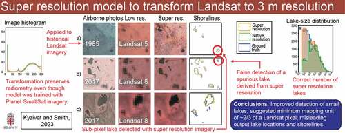
Landsat is the longest-running environmental satellite program and has been used for surface water mapping since its launch in 1972. However, its sustained 30 m resolution since 1982 prohibits the detection of small water bodies, which are globally far more prevalent than large. Remote sensing image resolution is increasingly being enhanced through single image super resolution (SR), a machine learning task typically performed by neural networks. Here, we show that a 10× SR model (Enhanced Super Resolution Generative Adversarial Network, or ESRGAN) trained entirely with Planet SmallSat imagery (3 m resolution) improves the detection of small and sub-pixel lakes in Landsat imagery (30 m) and produces images (3 m resolution) with preserved radiometric properties. We test the utility of these Landsat SR images for small lake detection by applying a simple water classification to SR and original Landsat imagery and comparing their lake counts, sizes, and locations with independent, high-resolution water maps made from coincident airborne camera imagery. SR images appear realistic and have fewer missed detections (type II error) compared to low resolution (LR), but exhibit errors in lake location and shape, and yield increasing false detections (type I error) with decreasing lake size. Even so, lakes between ~500 and ~10,000 m² in area are better detected with SR than with native-resolution Landsat 8 imagery. SR transformation achieves an F-1 score for water detection of 0.75 compared to 0.73 from native resolution Landsat. We conclude that SR enhancement improves the detection of small lakes sized several Landsat pixels or less, with a minimum mapping unit (MMU) of ~ ²/₃ of a Landsat pixel – a significant improvement from previous studies. We also apply the SR model to a historical Landsat 5 image and find similar performance gains, using an independent 1985 air photo map of 242 small Alaskan lakes. This demonstration of retroactively generated 3 m imagery dating to 1985 has exciting applications beyond water detection and paves the way for further SR land cover classification and small object detection from the historical Landsat archive. However, we caution that the approach presented is suitable for landscape-scale inventories of lake counts and lake size distributions, but not for specific geolocational positions of individual lakes. Much work remains to be done surrounding technical and ethical guidelines for the creation, use, and dissemination of SR satellite imagery.

GRAPHICAL ABSTRACT

KEYWORDS:

• SISR
• SRM
• size distribution
• object detection
• upscaling
• downscaling

1. Introduction

Landsat, the world’s longest-running environmental satellite program, began in 1972 and has retained 30 m spatial resolution since 1982 (Wulder et al. 2019). Landsat 5, 7, 8, and 9 satellites operated by NASA and the United States Geological Survey (USGS) have continuously collected data through five decades of operation, creating the world’s longest archive of satellite data from a single program. Since 2008, the existing archive and all future data were made available for free (Woodcock et al. 2011), also making the Landsat program the first to offer such a huge global image inventory without restriction or cost (Wulder et al. 2016). NASA and the USGS have a directive to continue the Landsat program through future satellite launches, further adding to its >7.5 million image archive (Wulder et al. 2016). Thus, the Landsat program is unprecedented in its longevity, availability, and continuity.

Landsat has been used for surface hydrology for decades (Smith 1997), but its 30 m resolution makes detecting small lakes and narrow rivers challenging (Yang and Smith 2016; Allen et al. 2018). This is a significant impediment to obtaining accurate lake inventories because lake-size distributions (LSDs, Downing et al. 2006) commonly follow power law distributions, making small lakes far more abundant than large ones, although there are exceptions (Muster et al. 2019). Power law behavior can only be modeled for lakes >0.3–0.46 km² (Kyzivat et al. 2019; Cael and Seekell 2016), so small lakes below this limit are therefore the most abundant but hardest to estimate by extrapolation. For this reason, improving the detection limit to ever-smaller lake sizes is an ongoing goal for hydrologic studies (Paltan, Dash, and Edwards 2015; Verpoorter et al. 2014; Messager et al. 2016; Kyzivat et al. 2019; Muster et al. 2019).

Individual pixels are not sufficient to detect lakes or their distributions, and must instead be grouped into objects. Raster map products like the Global Surface Water (GSW) suite (Pekel et al. 2016) use a minimum mapping unit (MMU) of one Landsat pixel, but a single water pixel is not guaranteed to be a lake. Vector classifications, which delineate discrete water bodies as objects typically have an MMU of several pixels, such as 40 pixels (40 m²) for airborne camera imagery (Kyzivat et al. 2019; Muster et al. 2019); 10 pixels (1,000 m² or 0.001 km²) for Sentinel-2 (Sui et al. 2022); 9 pansharpened, equivalent to 2 native pixels (0.002 km²) for Landsat 7 (Verpoorter et al. 2014); 4 pixels (0.0036 km²) for Landsat 8 (Paltan, Dash, and Edwards 2015); and 33 pixels (0.03 km²) for combined Landsat (Pi et al. 2022) imagery. While convention requires an MMU of 2–33 Landsat pixels (2,000–8,100 m²), such limits, in practice, still undercount small lakes, with high-resolution (HR) mapping showing that 70% of sampled northern lakes are smaller than 4 pixels and would thus be excluded (Kyzivat et al. 2018, 2019). These MMU selections follow a trend where fewer pixels are required for a confident lake detection as spatial resolution becomes coarser. A 1 km² pixel detection is unlikely to be false, for example, whereas a 500 m² pixel detection is more likely to be a lake, river fragment, cloud shadow, or terrain shadow. Therefore, there is a tradeoff between pixel resolution and per-pixel classifier accuracy, with greatest impact on small lakes sized near native pixel resolution.

Single image super resolution (SR) is an emerging machine learning tool for enhancing the pixel resolution of images and is increasingly being applied to remote-sensing imagery. Among the different SR models, generative-adversarial networks (GANs) produce results with greater perceptual quality and appear crisper to human observers than results from convolutional neural networks (CNNs, Wang, Bayram, and Sertel 2022). All supervised SR models, such as the one used here, require paired training images at different pixel resolutions. The ratio between these resolutions determines the output resolution and therefore the degree of SR enhancement. Remote-sensing SR imagery has been used to enhance object detection, using resolution ratios varying from 2 to 8×, to detect objects with several native resolution (hereafter: low resolution or LR) pixels in size. Shermeyer and Van Etten (2018) produce 2×, 4×, and 8× SR resampling ratios from 30 cm LR Worldview-3 imagery, which increases object detection average precision (AP) performance by ~ −2 to 11% points. Rabbi et al. (2020) use a 4× SR ESRGAN-based model on 30 cm and 1.2 m LR airborne imagery to detect cars (5 m length) and oil tanks (3 m diameter) with AP ranging from 77 to 95%. Courtrai, Pham, and Lefèvre (2020) use 8× SR to reconstruct realistic-looking and automatically detectable cars from just eight 1 m LR airborne and multi-source satellite pixels, with AP of 55 to 77%. Notably, previous SR object detection efforts focus on objects of uniform size still resolvable in LR imagery (e.g. vehicles and oil tanks). They have limited application to broad-scale remote sensing because they delineate only object bounding boxes, rather than counts or sizes; primarily use resampling ratios of ≤8× (Wang, Bayram, and Sertel 2022); and evaluate results on small image tiles, rather than mosaicked imagery. In sum, there is an opportunity to evaluate the detection of non-uniform sized objects as small as sub-pixels in remote sensing SR imagery, particularly at resolution ratios >8×, through landscape-scale metrics.

SR model training typically uses LR images derived from resampled (i.e. degraded) HR images (Sustika et al. 2020; Lezine, Kyzivat, and Smith 2021; Wang et al. 2018). Examples include the use of HR training data sets such as DIV2K (Agustsson and Timofte 2017; Ignatov et al. 2019) and UC Merced (Yang and Newsam 2010) image datasets. New methods are also emerging to use training images from other sensors with finer resolution, for example training Sentinel-2 imagery with Planet or Worldview imagery (Salgueiro Romero et al. 2020; Galar et al. 2020; Yoo et al. 2021) or Landsat 5 and 8 (Pouliot et al. 2018). Such cross-sensor training enables derivation of SR imagery from LR imagery possessing greater radiometric, spectral, and/or global observation frequency of the LR satellite, but requires meticulous image pre-processing. Previous 5× GAN (Salgueiro Romero et al. 2020) and 2×/4× CNN (Galar et al. 2020) studies trained SR models on paired LR Sentinel-2 and either Planet or Worldview HR images. To avoid learning a faulty SR transformation, they ensured precise image temporal and spatial alignment between training pairs, applying restrictive cloud filtering and image correlation thresholds. To date, cross-sensor studies have trained LR imagery only from Sentinel-2 (Salgueiro Romero et al. 2020; Galar et al. 2020; Yoo et al. 2021) not Landsat, and none demonstrate that their model can be applied to an independent sensor. A remote sensing SR model trained on HR and LR pairs from one sensor and evaluated against images from another would eliminate the labor of producing cross-sensor image pairs, but to our knowledge, none has been demonstrated.

We previously trained the SR GAN-based model Enhanced Super Resolution GAN (ESRGAN, Wang et al. 2018) on 289 global Planet HR image scenes, using 10× resampled HR images as the paired LR dataset (Lezine, Kyzivat, and Smith 2021). The SR model was prone to artifacts, including the realistic-looking, but spurious features observed by Wang, Bayram, and Sertel (2022). Even so, for Landsat-observable water bodies, the 10× SR model had similar high accuracy to a classification based on conventional, cubic-resampled imagery (Cohen’s kappa>0.97), and outperformed it with the detection of fine-scale shorelines. Remaining questions surrounding the utility of this model include its use for small lake, rather than shoreline, detection; proper interpretation of synthetic images, and especially its applicability to non-Planet LR input images, including from historical Landsat archives. Considering that GANs were originally developed to create fake imagery (Goodfellow et al. 2014), spurious features raise ethical concerns (Zhao et al. 2021) when being used to interpret and make decisions from SR imagery. To address these questions, we measure accuracy based on progressing filtering of small lakes to find an MMU for 10× SR imagery that represents a reliable size threshold to use for object detection.

Here, we use our 10× SR model previously trained from Planet images only (Lezine, Kyzivat, and Smith 2021) to test whether a Planet-trained SR model can be used to detect small and sub-pixel lakes in Landsat imagery. Our main goals are to: (1) Test whether an SR model trained from Planet can be successfully applied to Landsat; (2) Assess any improved detection of small lakes by determining the 10× SR minimum mapping unit (MMU); (3) Demonstrate SR on a historical Landsat 5 scene from 1985. To this end, we rely on object-, rather than pixel-based metrics to determine how well Landsat SR and LR lake detections agree with the number, size, and location of 25,523 Canadian and Alaskan lakes mapped from traditional airborne camera photography (Kyzivat et al. 2018, 2019; Walter Anthony and Lindgren 2021 Walter Anthony et al. 2021). First, we apply our Planet-trained model to Landsat LR imagery, and test for any unwanted transformation to the image radiometric values in the SR results. Next, we run the same threshold-based water classifier on both LR and SR Landsat imagery. Then, we evaluate the classifier against the independent airborne datasets using novel object-based and spatial metrics designed for remote sensing image mosaics. Finally, we demonstrate retroactive generation of SR imagery from a 1985 Landsat scene. We conclude with some recommendations for developing Landsat SR models, including an appropriate MMU for lake detection, and a caution on the ethical considerations raised by retroactive creation of SR imagery.

2. Data and methods

2.1. Airborne and Landsat remote-sensing imagery

A study domain from the NASA Arctic-Boreal Vulnerability Experiment (ABoVE, Miller et al. 2019) was chosen based on the availability of extensive HR, lake vector datasets to be used for independent verification of Landsat LR and SR lake detections. Kyzivat et al. (2019, 2019) provide 1 m resolution color-infrared camera orthomosaics and a lake map acquired concurrently with AirSWOT Ka-band radar data (Fayne et al. 2020), a prototype of the forthcoming Surface Water and Ocean Topography (SWOT) satellite mission. The lake map, which was derived from a semi-automated, unsupervised classifier, has a 40 m² (40 pixels) native MMU and a maximum lake size of 15.5 km². Classification errors are largely due to roads, agricultural fields, and clouds/haze, with the latter impacting 28% of the camera product’s image tiles. The lake map has a user’s accuracy (precision) of 87.1%, a producer’s accuracy (recall) of 94.0%, and a geolocation error of ≤14.7 m RMSE relative to a Digital Globe base map for 90% of the dataset (Kyzivat et al. 2019). From 23,280 km² of camera imagery acquired over 13 regions for the 2017 ABoVE AirSWOT flights, we selected portions of 10 lake-rich regions encompassing 23,212 km² to use for SR lake detection (Figure 1). All image processing was carried out in Python 3.9, using the open-source packages numpy (Harris et al. 2020), scipy (Virtanen et al. 2020), sckikit-learn (Pedregosa et al. 2011), gdal (Contributors 2022), rasterio (https://github.com/rasterio/rasterio), geopandas (Jordahl et al. 2020), and NASA DELTA (https://github.com/nasa/delta). To comply with previous convention (Wang et al. 2018; Rabbi et al. 2020), we refer to this selected, HR lake map as a “ground truth” (GT) dataset, even though the AirSWOT camera is an airborne sensor.

Figure 1. Study regions are derived from available HR vector lake maps created for the NASA Arctic-Boreal Vulnerability Experiment (ABoVE) (Kyzivat et al. 2018, 2019; in red); and a historical study of permafrost lake change (Walter Anthony et al. 2021, in blue).

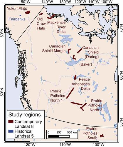
Fourteen Landsat 8 scenes were downloaded as Collection 2, level 2 (surface reflectance) products over the identified regions (Figure 1). Scenes were selected based on the closest temporal acquisition to the 2017 AirSWOT flights (3–27 days) with <5% cloud coverage. All scenes were classified as Tier 1, signifying the best available geolocation error of ≤12 m RMSE. In preparation for the ESRGAN model, which operates on 8-bit imagery, scenes were converted from 16-bit to 8-bit integers, using an image stretch based on the 1 and 95 percentiles of cloud-free pixels to emphasize radiometric contrast between land and water. Finally, scenes were mosaicked (if necessary) and tiled to 48-pixel square tiles with 16 pixels overlap (Figure 2) within buffered outlines of the 10 study regions (Table S1).

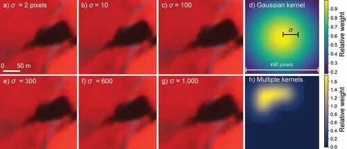
Figure 2. Sensitivity test for standard deviation of Gaussian smoothing kernel used for image reconstruction varying from 2 pixels (a) to 1,000 pixels (g). Seamlines are visible near the image center-left and and/or center-bottom for all standard deviation values except 10 and 100, so an intermediate value of 30 was chosen. Center coordinates are 52.6563° N, 107.08323° W. Panel (d) illustrates of the weights of a single kernel, and (h) illustrates the superposition of multiple kernels, used to normalize the resulting image. Panels (d) and (h) are 480 pixels square and are schematics not associated with a particular geographic location.

2.2. Lake detection in super and native resolution Landsat imagery

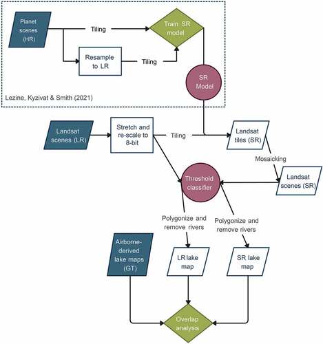
Landsat SR imagery was derived from the Landsat native resolution (i.e. LR) image tiles using the Planet-trained ESRGAN 10× SR model of 2020), which operates on near-infrared (NIR), green (G) and red (R) 3-band images and is modified from ESRGAN (Wang et al. 2018). This model was first trained on HR images from the DIV2K dataset (Agustsson and Timofte 2017; Ignatov et al. 2019) and then on ~183,000 48-pixel square tiles from 289 Planet scenes (Lezine, Kyzivat, and Smith 2021), using paired training LR images derived via bicubic resampling. Thus, these artificially coarsened LR images were free from the confounding factors in cross-sensor super resolution (Salgueiro Romero et al. 2020; Galar et al. 2020) but could not be used to demonstrate SR on actual Landsat images, as we do here. The accuracy of this model was previously assessed at 27.36 peak signal-to-noise ratio (PSNR) compared to 35.06 for a 4× model and it was used to demonstrate enhanced shoreline detection from SR images as compared to bicubically resampled images against native Planet resolution (Lezine, Kyzivat, and Smith 2021). When applied to Landsat, the model produced SR tiles of dimension 480 × 480 pixels, corresponding to a 3 m ground sample distance per pixel (commensurate with 3 m resolution Planet imagery). To reconstruct SR versions of the cropped Landsat scenes, output SR tiles were mosaicked using a radial Gaussian weighting kernel (Figure 2d) that blended values from multiple tiles (Figure 2h) in overlapping tile edges. Trial and error (Figures 2a–, e–) showed that both 10- and 100-pixel Gaussian standard deviation prevented seamlines between tiles, so their rounded geometric mean of 30 was used for mosaicking. This procedure was applied in batch over all Landsat scenes.

Reconstructed Landsat SR scenes were evaluated for radiometric consistency using several statistical tests. First, for visual inspection, image histograms for each band of corresponding LR and SR Landsat scenes were plotted. Next, a Kolmogorov – Smirnov test was used to compare corresponding distributions. Finally, mean band values for LR and SR were calculated over each image and used for the Wilcoxon signed-rank test, a nonparametric comparison between population means that assumes no underlying distribution.

To classify surface water in both SR and LR Landsat images, near-infrared band thresholds for each scene were chosen based on visual assessment following Yamano et al. (2006) and Muster et al. (2017), without reference to ground truth. This one-parameter (band threshold) method, implemented in ENVI 5.6.1, was chosen for its simplicity, which permits comparison between image resolutions, not classifiers. Only the LR images were used to choose thresholds (Table S1), which were verified on corresponding SR images by confirming that the segmentation delineated a reasonable number of lakes without fragmentation near their shorelines (examples of unavoidable fragmentation caused by shadows are in Figure 5b). In sum, the classifier enables verification and modification of thresholds, if needed, and it can be exactly replicated on images of different spatial resolutions, which is crucial for further statistical comparisons.

Finally, the pixel-based SR and LR water classifications were converted to vector objects. First, water pixels were polygonized, and morphological closing (i.e. successive outwards, then inwards buffering) was performed to aggregate adjacent lake fragments. Based on Kyzivat et al. (2019), a conservative 10 m element was used for the morphological closing, which aggregated any lake fragments within 20 m of each other, which are assumed to have their connections obscured by vegetation. Next, the river mask of Kyzivat et al. (2022) was expanded to cover the remaining regions and used to remove rivers. Finally, lake polygons were clipped to a region of interest (ROI) defined as the intersection of the original Landsat and AirSWOT camera scene boundaries. Any fractional lakes that overlapped scene boundaries or resulted from clipping out the river mask were retained to preserve a large sample size. For consistency, the same river removal and ROI cropping were applied to the GT lake polygons, and the resulting polygons thus included lakes detected in LR, SR, and GT, all with a common ROI and a 40 m² native MMU (Figure 3).

Figure 3. Flow chart of image processing, super resolution transformation, classification and overlap analysis. Inputs are in teal parallelograms, analyses are in green diamonds, and models are in red circles. HR refers to high resolution, LR to low resolution, and GT to ground truth.

2.3. Evaluation of lake object detection performance

To assess lake geolocation accuracy, three fine-scale metrics were calculated to compare SR versus LR object detections against GT: precision (true positives as a fraction of total GT lakes, Equation 1[1] $P=\frac{TP}{TP+FP}$[1] ), recall (true positives as a fraction of all identified lakes, Equation 2[2] $R=\frac{TP}{TP+FN}$[2] ), and F-1 score (the harmonic mean of precision and recall, Equation 3[3] $F_1=\frac{2}{\frac{1}{P}+\frac{1}{R}}$[3] ). We consider these metrics fine-scale because they are only computed between two objects at a time. True positives (TPs) were defined as lake objects in SR (or LR) that overlapped or fell within 30 m of a GT lake object. This 30 m tolerance was chosen based on the 30 m Landsat pixel size, the known geolocation accuracies of LR (12 m) and GT (14.7 m), and the expectation that sub-pixel SR lakes would not necessarily overlap GT lakes but should nonetheless count as valid detections if they are located within a small tolerance. Type I error (commission) was assessed through Precision and Type II error (omission) through recall as follows:

[1] $P=\frac{TP}{TP+FP}$[1]

[2] $R=\frac{TP}{TP+FN}$[2]

[3] $F_1=\frac{2}{\frac{1}{P}+\frac{1}{R}}$[3]

where FP are false positives and FN are false negatives, P is precision, R is recall, and F₁ is F-1 score. All three metrics vary from 0 to 1, with 0 indicating no overlap and 1 indicating perfect agreement. To compare LR and SR object detections to GT, they were calculated for all study regions in aggregate.

To find an appropriate MMU to use for error assessment and to reduce uncertainty through averaging, these fine-scale metrics precision, recall, and F-1 score were computed over a variety of distance and size thresholds. First, to find a reliable MMU, a series of truncated datasets were created (referred to as the full GT comparison) by progressively filtering out LR and SR lakes based on 20 logarithmically spaced minimum sizes ranging from 40 to 10⁷ m². Ranges were chosen based on the native GT MMU and the largest observed lakes. These fine-scale metrics were computed at each threshold, and since precision and recall were monotonic, F-1 score had a clear maximum and was used to determine the MMU as the lake size threshold that maximized it (Figure 6a–). Next, truncated datasets were again created, except GT lakes were included in the truncation (referred to as the truncated GT comparisons, Figure 6d–). Given this equal truncation of datasets, results could be used to determine classifier performance at the MMU or at any size threshold. Finally, similar to previous studies (Shermeyer and Van Etten 2018; Courtrai, Pham, and Lefèvre 2020), averages of the fine-scale metrics precision, recall, and F-1 score (AP, AR, and AF1) were computed over distance tolerances varying from 0 m to 30 m in 5 m increments. These estimates and following summary statistics were computed at the determined MMU for 10× SR, which represents the smallest-sized lake for which errors of commission and omission are balanced.

Lakes vary considerably in size, necessitating scale-independent metrics that can be applied across image tiles to evaluate lake sizes and counts. We modeled the lake-size distribution (LSD, Cael and Seekell 2016; Kyzivat et al. 2019) as a power law (Clauset, Rohilla Shalizi, and Newman 2009; Virkar and Clauset 2014; Horvat et al. 2019) to observe any effects from increased spatial resolution. A power law distribution has the property of scale invariance (Cael and Seekell 2016) and takes the form:

[4] $P\left(a>A\right)=C{A}^{-\alpha }$[4]

where A is a given lake area, and C and α are fitted constants. The best-fitting power law was obtained using the python powerlaw package, which first finds the optimal minimum value A₀ for the onset of power law behavior by minimizing the Kolmogorov – Smirnov distance between the data and fit over potential A₀ values (Alstott, Bullmore, and Plenz 2013). The parameter α is fit for the optimal A₀ using a maximum likelihood estimator, and the Kolmogorov – Smirnov test is subsequently run to find a p-value for a power-law fit compared to the null hypothesis of an exponential distribution. The fitted SR and LR LSDs were evaluated against that of GT based on mean and median lake sizes and fitted power law parameters.

2.4. Retroactive application of SR to a 1985 Landsat 5 image

To assess retroactive application of a Planet-trained SR model to older Landsat imagery, a 31 August 1985 Landsat 5 scene (Table S1) was chosen to correspond to an air photo-derived lake shoreline dataset for Fairbanks, AK, USA from 23 December of the same year (Walter Anthony and Lindgren 2021). Like the contemporary GT dataset, lake shorelines in this historical GT dataset were derived using semi-automated, object-based image classification and were manually edited to remove rivers (Lindgren et al. 2016, 2019). Although this dataset has a minimum lake size of 13 m², we truncated it to 40 m² for consistency with the modern GT dataset. Identical image processing and statistical analysis, as described in Sections 2.1-2.4, were applied to the corresponding Landsat 5 scene, except an ROI was manually drawn to exclude frequently misclassified urban areas surrounding Fairbanks. This processing produced 242 historical GT lakes from the year 1985 ranging from 40 m² to 0.10 km² in area.

3. Results

3.1. Radiometric consistency

Comparison of SR and LR pixel value frequency distributions reveals a generally good match between LR and SR with no difference in mean band values (Figure 4), and image coloration appears unchanged (Figure 5). The Wilcoxon signed-rank test showed no statistical difference in mean per band over the 11 scenes (p = 0.31), with an anomaly of −4.7, 1.7, and −0.4 DN units compared to LR band means for (N, G, and R bands, respectively). Even so, each histogram pair was determined statistically distinct by the highly sensitive Kolmogorov – Smirnov test (p = 0). Thus, the SR transformation can subtly change the pixel distributions but does not introduce a bias in mean band value.

Figure 4. Example pixel frequencies for Yukon Flats, Alaska (a-c), Canadian Shield near Baker Creek (d-f), and Fairbanks, AK 1985 (g-i). Bin counts are normalized to facilitate comparison between data sets of different sizes. Jagged Landsat 5 histograms are a result of the 1–95% image stretch applied to native 8-bit radiometric resolution. In contrast, the SR transformation produces smooth histograms that make use of the total dynamic range.

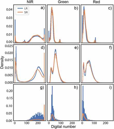
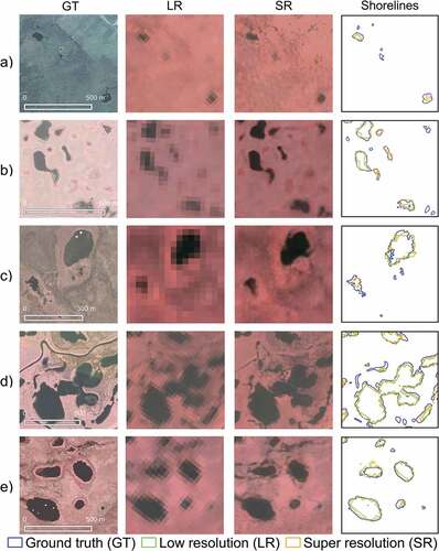
Figure 5. Airborne camera GT and Landsat LR and SR examples demonstrate the advantages and limitations of SR in Fairbanks, Alaska, 1985 (a); Prairie Potholes South, North Dakota (b); Canadian Shield Margin, Northwest Territories (c); Mackenzie River Delta, Northwest Territories (d); and Old Crow Flats, Yukon territories (e). In row (a), an additional lake is detected in SR compared to LR for Landsat 5 data from 1985. In (b), the lake in the northeast corner has an SR lake detection within thirty meters of GT, showing how use of an adjacency buffer better evaluates results. Several lakes fragmented into two in the SR classification, altering the abundance but not total area of lakes. In row (c), SR classification detects one lake missed in LR, but both classifiers miss three lakes sized near the native GT MMU. In row (d), several small GT lakes are not detected in either Landsat resolution. A river in the top of the image is successfully masked out and therefore does not contribute to summary metrics. In row (e), all lakes detected in SR are also detected in LR, and there are two false positive SR lakes generated near the image center. Center coordinates: 64.8775, −147.7242 (a); 47.1432, −99.2494 (b); 63.7498, −117.6939 (c); 68.2699, −134.4791 (d); 67.8731, −139.9617 (e).

3.2. Determination of an appropriate minimum mapping unit (MMU) for Landsat SR imagery

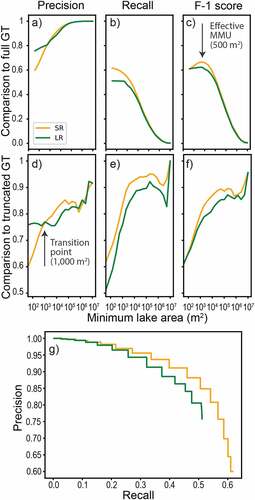
An optimal MMU of 500 m² was identified for lake detection in Landsat SR imagery and used to compute metrics for both resolutions. From the full GT comparison used for sensitivity analysis, SR F-1 score peaks at this lake size (Figure 6c), signifying best tradeoff between type I and II errors for lakes of this size. LR also has a subtle maximum around 40–1,000 m², but we do not consider it robust enough to unequivocally state an LR MMU, a task that we defer to previous studies. The observed overall similarity in SR and LR F-1 curves despite a 10× difference in spatial scale suggests that this property is largely independent of pixel size and likely tied to intrinsic sensor resolution. Therefore, from the F-1 score plot (Figure 6c), we identify an optimal MMU of 500 m² (²/₃ Landsat pixel) for 10× SR lake detection and use this MMU for subsequent metrics for both SR and LR.

Figure 6. Accuracy metrics for different minimum lake sizes indicate that recall and F-1 scores are greater for Landsat SR than LR for all lake sizes (e, f), while precision varies and is less for SR than LR for small lakes until a transition at 1,000 m² (d). An effective MMU of 500 m² (²/₃ of a Landsat pixel) is determined based on the global maximum of F-1 score in (c). Metrics are calculated against all GT lakes (a-c), and for GT lakes only above the corresponding lake size threshold (d-f), with the latter curves being noisier due to the sample size decreasing with size threshold. The precision-recall curve (g) is plotted using data in (d-f), and the SR classification has a greater area under the curve (0.57) than that of LR (0.48).

3.3. Detection of small lakes in contemporary Landsat SR imagery

SR imagery detects small lakes more reliably than does LR (Figure 5). Despite inferior precision for lakes < ~1,000 m² (~1 Landsat pixel), the SR classifier yields superior recall, and F-1 scores for lakes <10,000 m² (~10 Landsat pixels, Figure 6a–). SR and LR AF1 scores are 0.75 and 0.73, respectively, for lakes larger than the 500 m² MMU (Table 1). In addition, the area under the precision-recall curve (Figure 6g) is greater for SR (0.57) than for LR (0.48), implying improved performance, even when averaged over all 20 minimum lake size thresholds used to compute it. The high precision (low type I error) of LR in detecting small lakes can be attributed to under-sampling of small lakes in the LR dataset. In this size range, only the LR lakes with the darkest NIR values are detected, and as a result, they are unlikely to be false positives. In contrast, SR false positives are more common due to confusion with roads, shadows, and fragments of rivers not included in the river mask. In sum, more small lakes can be detected in SR than in LR imagery, but at the expense of some false detections, leading to modest gains overall.

Table 1. SR lake detections have better skill than LR for lakes larger than 500 m², as measured by Average Recall (AR) and F-1 score (AF1), but not by Average Precision (AP), when compared against GT.

		AP	AR	AF1
Landsat 8	LR	0.75	0.71	0.73
	SR	0.74	0.77	0.75
Landsat 5	LR	1.00	0.31	0.47
	SR	0.98	0.43	0.60

The SR water classification yields a remarkably accurate number and size distribution of lakes if all potential lake detections are included (Figure 7a). From 25,281 GT lakes, 25990 are detected in SR (+2.8% difference) and 17,059 in LR (−33% difference, Table 2). SR outperforms LR in estimating the count and mean and median lake size, which agree with GT by+7.7 and+37%, respectively, and represent significant improvements over LR (+72% and+711%, respectively). A lake-size distribution histogram based on only true positives shows improved agreement compared to the LR histogram, especially for smaller lake sizes (Figure 7b). It is evident that many of these correctly sized lakes are located outside of the 30 m tolerance used to define a true positive. For lakes larger than the 500 m² MMU, the classifier obtains a 78.1% recall over all remaining size bins (Figure 6e). If this tolerance is relaxed to 90 m, the recall for SR increases to 83.8%, signifying that about ¹/₃ of these false-positive lakes are “near misses” within 90 m (Figure 8b). Overall, SR lakes show good agreement with GT in number and size, representing significant improvements over LR.

Figure 7. Lake-size distribution histograms based on all detected lakes (a, c) show good agreement between the size frequencies of SR and GT lakes for contemporary Landsat 8 scenes (a, b) and historical Landsat 5 scenes (c, d). When only plotting true positive lakes (b, d), this agreement is diminished, although SR still detects more lakes than LR in nearly all size bins up to 10,000 m² for both recent (b) and 1985 (d) Landsat imagery. Removing rivers occasionally led to LR lakes counterintuitively smaller than one 900 m² Landsat pixel (a, b). These lakes were nevertheless retained to follow consistent geoprocessing steps for all datasets.

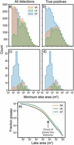
Figure 8. Accuracy metrics for different tolerance distances to 90 m based on the MMU of 500 m². Table 1 reports mean statistics using tolerances ≤ 30m.

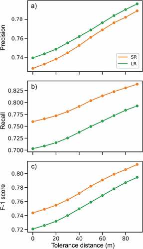
Table 2. Scale-independent lake detection metrics of count (N), true positives, lake area, and power law parameters A₀ (optimal onset of power law behavior) and α (fitted power law slope).

Resolution	N	N (greater than MMU)	True positives	Mean lake area (m^2)	Median lake area (m^2)	α*	A0* (m^2)
GT	25,281	14,522	-	54,639	899	2.151 ± 0.061	536,738
LR	17,059	15,226	10,533	93,988	7,288	2.197 ± 0.056	471,756
SR	25,990	13,947	11,339	58,835	1,235	2.194 ± 0.069	698,115
GT**	43,562	23,178	-	137,000	665	1.89 ± 0.04	343,074

*All reported α and A₀ values have statistical significance at a 0.001 significance level. **A comparison is made to Kyzivat et al. (2019), who use a similar domain to GT, but correct for large lakes not completely observable by the narrow airborne swaths examined here.

Power law LSD behavior is evident for larger lakes at all three resolutions, as indicated by a constant slope when plotted as a survival function in log-log space (Figure 7e). Fitted truncated power laws (Clauset, Rohilla Shalizi, and Newman 2009) show no significant difference in the power law exponent α or minimum size A₀ among all image resolutions (Table 2). Even so, the SR LSD is a better approximation than the LR LSD, which has a power law slope matching GT for the large lakes where it can be computed, but exhibits slope deviations for small lakes (Figure 7e). Thus, the SR-derived LSD closely matches the GT LSD, offering significant improvement over the LR-derived LSD.

3.4. Detection of small lakes in historical Landsat SR imagery

SR lake detection was also successfully demonstrated for a 1985 Landsat 5 scene over Fairbanks, Alaska, USA. Like with Landsat 8, SR lake detections have inferior precision, but superior recall and F-1 scores compared to LR lake detections (Table 1). Compared with Landsat 8 statistics, the 1985 Landsat 5 SR scene yields superior precision (AP = 0.98 for Landsat 5, vs. 0.75 for Landsat 8) but inferior recall (AR = 0.43 vs. 0.77) and F-1 score (AF1 = 0.60 vs. 0.75) (Table 1). Notably, SR lake detection yields only one false positive in this scene, and LR yields none, producing higher AP values than the Landsat 8 scenes. The low AR and AF1 values are likely due to the finer native resolution of the historic Fairbanks shoreline dataset (minimum lake size of 13 m², Lindgren et al. 2016) than the contemporary GT dataset (40 m² minimum, Kyzivat et al. 2018), even though both were ultimately truncated to 40 m² for plotting and to 500 m² for summary metrics. Since the historical GT dataset has higher native resolution than the contemporary GT dataset, these differences in AR and AF1 are likely a product of GT dataset comprehensiveness, not of Landsat sensor properties.

4. Discussion

4.1. Significance of results

Here, we demonstrate that a 3 m SR model trained solely on Planet SmallSat imagery can be used to super-resolve 30 m contemporary and historical Landsat imagery to detect small Arctic-boreal lakes at sub- to several-pixel scales. Our cross-sensor application of SR to lake mapping is an advance over previous practices in at least three ways: 1) it quantifies an SR MMU for lake object detection and finds the MMU is an improvement from LR imagery; 2) it assesses error using fine-scale and scale-independent object-based metrics, finding remarkable concordance in lake abundance and size distribution; and 3) most significantly, it shows that a model trained by degrading HR imagery to obtain LR (here, 3 m resolution Planet SmallSat imagery, degraded to 30 m) can be successfully applied to a different LR instrument (here, contemporary and historical 30 m Landsat imagery). Because our approach performs cross-sensor training using only one sensor (i.e. Planet), this advance is of particular value to the Landsat archive, which long predates widely available HR imagery.

Our results suggest that Landsat 10× SR provides little improvement in precise geolocational mapping of small lakes, yet some improvement to overall lake detection. Gains caused by improved spatial resolution are offset by increases in false-positive detections, of which ~¹/₃ are “near misses” (i.e. 35% are located within 30–90 m of real-world lake, Section 3.3). Despite these geolocational errors, improvements in overall lake detection (Table 1) are evident, depending on which metric and error types are considered. Our observed reduction in AP caused by SR is on par with the outer range of Shermeyer and Van Etten (2018), who found typical mean average precision (mAP, a multi-class analog to AP) ranging from 0.55 to 0.59, representing an increase in mAP of −0.2 to 0.11 compared to LR object detection for various resampling ratios. The 8× SR model of Courtrai, Pham, and Lefèvre (2020) had an AP of 0.55 to 0.77 and an F-1 score of 0.03 to 0.86, with no available GT at that resolution for comparison. Our contemporary Landsat AP of 0.75 (LR) and 0.74 (SR) for a 10× resolution ratio (Table 1) falls within the range of these two previous studies, both in magnitude and in lack of SR performance gain. In both studies, the objects being detected were larger than ~5 LR pixels and used resolution ratios ≤8×, with objects in Shermeyer and Van Etten (2018) typically between 10 and 50 pixels. In contrast, our smallest detectable lakes are of subpixel size, which explains why SR produces a decrease in AP in our study, while this was a rare occurrence for Shermeyer and Van Etten (2018). Neither of these studies report AR, which measures type II error and can be just as important as type I error, depending on the application (Matsuda et al. 2005). Based on AR and AF1, we show modest improvement in SR lake detection and localization with our suggested MMU of 500 m² offering the best tradeoff between type I and II error.

Our quantification of cross-sensor performance using scale-independent metrics, such as the lake-size distribution (LSD), offers additional scientific benefits beyond Landsat SR performance assessment. In particular, SR imagery can help determine whether observed slope breaks in LSD plots are due to sensor resolution or to a physical process in lake formation. Using airborne camera imagery, Kyzivat et al. (2019) find an onset of power law behavior at 343,074 m², which is in general agreement with our results of 536,738 to 698,115 m² (Table 2). This size limit is within the range of MMUs of 2,000 m² − 30000 m² (2–33 pixels) from previous studies (Pekel et al. 2016; Kyzivat et al. 2019; Muster et al. 2019; Sui et al. 2022; Verpoorter et al. 2014; Paltan, Dash, and Edwards 2015; Pi et al. 2022) and well above our own recommendation of ²/₃ of a pixel for SR Landsat imagery. This high size limit indicates that the onset of power law behavior is a true geophysical phenomenon, not an artifact of sensor resolution. Thus, scale-based lake estimates cannot be improved by increasing spatial resolution, and SR is better used for direct lake counting.

The main value added by applying an SR model to Landsat imagery is improved lake counts and size distributions, particularly for small lakes sized around one to several pixels. For example, even when truncating all datasets to 40 m², our LR classifier still detects fewer lakes than both GT and SR, particularly for small lakes up to 8,000 m² or 11,000 m² (~9–12 pixels) depending on whether false positives are included (Figure 7a) or excluded (Figure 7b). As expected, our LR classifier under-counts lakes smaller than the conventionally used LR Landsat MMU (2,000–30,000 m² or~2–33 pixels, Section 1). SR thus offers a remedy for this under-counting by improving the reliable MMU for LR imagery four-fold and yielding unbiased estimates of lake count. Although not always improving geolocational accuracy, SR can be used for estimating the overall bulk size distribution and abundance of Arctic-boreal lakes.

The most promising aspect of our cross-sensor SR study its successful application to historical Landsat 5 imagery (Figures 4, 5, 7). We show that this application yields improved detection of small lakes based on a simple, threshold-based image classification (Figure 6, Table 1). To our knowledge, no historical object detection from SR has been previously shown or evaluated, although Pouliot et al. (2018) also derived SR images from Landsat 5 trained against modern-era HR Sentinel-2 data. Our SR transformation produces a small but statistically insignificant bias in radiometric values, consistent with Lezine, Kyzivat, and Smith (2021), who reports a negative or zero pixel value bias, and with Salgueiro Romero et al. (2020, Figure 6 within) whose cross-sensor SR model produces little change in image histogram shape. Thus, the SR transformation from ESRGAN (and perhaps other) models appears to have little impact on image radiometric properties, even across sensors. Importantly, unlike Salgueiro Romero et al. (2020) and other cross-sensor SR studies (Galar et al. 2020; Yoo et al. 2021), our model was trained with imagery derived from only one sensor (Planet), yet could still be transferred to another sensor (Landsat), opening up the possibility of further retroactive generation of SR.

4.2. Ethical considerations of super resolution object detection

Our retroactive generation of super resolution (SR) imagery for a time when no satellite HR imagery was publicly available raises interesting ethical concerns about the production and use of satellite SR imagery. First, there is a human proclivity to regard image data, particularly from high-resolution (HR) satellite images, as accurate, neutral, or politically uncharged (Bennett et al. 2022). This proclivity is concerning when considering that satellite SR images are commonly derived from GANs, models originally designed to create synthetic, or fake, data (Goodfellow et al. 2014). A known byproduct of ESRGAN (Wang et al. 2018) and other GAN-based models (Wang, Bayram, and Sertel 2022), for example, is their tendency to produce spurious but seemingly realistic image features (e.g. Lezine, Kyzivat, and Smith 2021), as shown in Figure 4e. GANs and other artificial intelligence models used in earth observation also suffer from a lack of explainability (Gevaert 2022), which can make users less likely to evaluate their uncertainties. While the ethical consequences of misplaced Arctic-boreal lakes shown here are innocuous, both type I and type II errors in other applications of SR object detection, such as intelligence gathering (e.g. Shermeyer and Van Etten 2018) could have serious ramifications. A related concern is the deliberate use of SR satellite images to mislead or disseminate disinformation, for example, with geographic deep fakes (Xu and and Zhao 2018; Zhao et al. 2021). Put simply, there is an innate allure to high spatial resolution imagery that human interpreters should be cognizant of when viewing retroactive SR satellite products for which no independent HR information is available for verification. We therefore caution that the approach presented here may safely be applied to assess bulk lake count inventories and size distributions (LSDs), but not to determine specific geolocational positions or areas of individual lakes.

4.3. Limitations and future work

Small lakes are more readily detected in SR than in LR imagery, but at the expense of more false detections. To balance these effects and increase reliability, we suggest considering only those objects larger than our suggested 10× Landsat SR MMU. Given an MMU of ~ ²/₃ of Landsat pixel, 10× super resolution appears to be an unnecessarily high resolution ratio for hydrological mapping, and 2× or 4× ratios may be just as effective. Although absolute measurements of accuracy (e.g. AF1 of 0.75 and 0.73 for SR and LR, respectively) are sensitive to the chosen 30 m tolerance distance, this tolerance improves both SR and LR results equally, and thus relative comparisons between datasets or lake size thresholds are still valid. Results could also be improved by incorporating multi-temporal inputs using techniques from image fusion (Zhao and Liu 2022). While we here degraded the radiometric resolution of Landsat-8 to 8-bit data in preparation for the SR model, future investigations should make full use of the native 16-bit radiometric resolution of Landsat 7–9 for contemporary SR studies. Our GT dataset derived from narrow airborne flight lines cannot detect large lakes in their entirety, and we made no attempt to correct for associated impacts on LSD (Kyzivat et al. 2019). This study’s first demonstration for a single Landsat 5 SR image leaves abundant opportunities for future studies comparing larger Landsat 5 datasets with historical air photos, maps, or other fine-scale information. Finally, we note a dearth of ethics studies examining the creation, use, and dissemination of SR satellite imagery, and hope our brief discussion prompts future work in this area.

5 Conclusion

The major contributions of this study are summarized as follows:

• We provide an early example of historical super resolution (SR), including from Landsat 5.

• We evaluate the use of 10× SR images for object detection and localization for lakes ranging from sub-pixel to thousands of pixels in size.

• We systematically test a minimum mapping unit (MMU) for SR lake detection, considering both fine-scale (precision, recall, F-1 score) and scale-independent metrics (lake abundance, size distribution, onset of power law behavior).

• We evaluate SR imagery on an independent sensor not used for training and test for any bias in radiometric values.

• We describe a blended tiling method to reconstruct satellite scenes from output tiles produced by SR models.

Here, we demonstrate generation of 3 m super resolution (SR) imagery from archived 30 m Landsat imagery, using a general adversarial network (GAN) trained entirely with independent, high-resolution (HR) Planet SmallSat imagery. This cross-sensor generation of SR is unique in not requiring time-intensive image cross-normalization techniques, and in seeking to detect small objects (lakes) at sub- to several-pixel scales. Furthermore, we show the reliable detection of lakes in Landsat 5 and 8 imagery as small as ~²/₃ of a Landsat pixel (500 m²), a significant improvement over the 2–33 pixel limit typically used for native resolution Landsat imagery. The super-resolved 3 m resolution of Landsat SR imagery does not adversely impact radiometric values, introducing only a small, statistically insignificant bias. Total SR lake counts agree within a remarkable +2.8% of ground truth (GT) if false positives are allowed and −55% if they are excluded. In contrast, total lake counts from native-resolution (30 m) Landsat imagery agree within −32%, and −58%, respectively. Compared to unenhanced imagery, an SR transformation improves the type II error (recall) and F1-score of lake detection, but not the type I error (precision) for both Landsat 5 (1985) and 8 (2017). Type II error has been largely overlooked by previous studies but is more relevant than type I error for assessing lake abundance. From this early demonstration, we conclude that classifications of cross-sensor SR improve estimates of the overall abundance and size distribution of lakes, and that onset of power law behavior in lake size distributions (LSDs) is a true geophysical phenomenon, not an artifact of sensor resolution. Even so, SR-derived lake maps contain “realistic-looking” errors in lake geolocation and shoreline details that human observers should be wary of. They should thus be interpreted with caution and are best used for bulk estimation of total lake abundance and LSD. Much work remains surrounding the creation of SR models, their retroactive application to historical satellite imagery, and formulation of ethical guidelines for the production, interpretation, and use of SR images.

Author contributions

E.D.K. carried out the analysis and L.C.S. provided guidance. Both authors designed the study and reviewed the final manuscript.

Availability of data and code

Code and data used for this analysis are available on GitHub (https://github.com/ekcomputer/pixel-smasher) and Zenodo (https://doi.org/10.5281/zenodo.7306219).

Acknowledgments

The authors would like to thank Ekaterina Lezine and Prof. Karianne Bergen for helpful guidance.

Disclosure statement

No potential conflict of interest was reported by the authors.

Supplementary material

Supplemental data for this article can be accessed online at https://doi.org/10.1080/15481603.2023.2207288.

Additional information

Funding

This work was funded by the NASA Terrestrial Hydrology Program (grant number 80NSSC20K0429) managed by Dr. Jared Entin, a Future Investigators in NASA Earth and Space Science and Technology (FINESST) fellowship managed by Dr. Allison Leidner (grant number 80NSSC19K1361), and the NASA Terrestrial Ecology Program (grant number 80NSSC22K1237) managed by Dr. Hank Margolis.

References

- Agustsson, E., and R. Timofte. (2017). NTIRE 2017 Challenge on Single Image Super-Resolution: Dataset and Study. IEEE Computer Society Conference on Computer Vision and Pattern Recognition Workshops, 2017 July, 1122–17. 10.1109/CVPRW.2017.150
- Allen, G. H., T. M. Pavelsky, E. A. Barefoot, M. P. Lamb, D. Butman, A. Tashie, and C. J. Gleason. 2018. “Similarity of Stream Width Distributions Across Headwater Systems.” Nature Communications 9 (1): 610. doi:10.1038/s41467-018-02991-w.
- Alstott, J., E. Bullmore, and D. Plenz. 2013. Powerlaw: A Python Package for Analysis of Heavy-Tailed Distributions. doi:10.1371/journal.pone.0085777.
- Anthony, K. W., and P. Lindgren. 2021. ABoVe: Historical Lake Shorelines and Areas Near Fairbanks, Alaska, 1949-2009. Oak Ridge, Tennessee, USA: ORNL DAAC. doi:10.3334/ORNLDAAC/1859.
- Anthony, W., P. Lindgren, P. Hanke, M. Engram, P. Anthony, R. P. Daanen, A. Bondurant, et al. 2021. “Decadal-Scale Hotspot Methane Ebullition Within Lakes Following Abrupt Permafrost Thaw.” Environmental Research Letters 16: 35010. doi:10.1088/1748-9326/abc848.
- Bennett, M. M., J. K. Chen, L. F. Alvarez, and C. J. Gleason. 2022. “The Politics of Pixels: A Review and Agenda for Critical Remote Sensing.” Progress in Human Geography 46 (3): 729–752. doi:10.1177/03091325221074691.
- Cael, B. B., and D. A. Seekell. 2016. “The Size-Distribution of Earth’s Lakes.” Scientific Reports 6 (29633). doi:10.1038/srep29633.
- Clauset, A., C. Rohilla Shalizi, and M. E. J. Newman. 2009. “Power-Law Distributions in Empirical Data.” SIAM Review 51 (4): 661–703. doi:10.1137/070710111.
- Contributors, G. D. A. L. /. O. G. R. 2022. “GDAL/OGR Geospatial Data Abstraction Software Library.” doi:10.5281/zenodo.5884351.
- Courtrai, L., M. -T. Pham, and S. Lefèvre. 2020. “Small Object Detection in Remote Sensing Images Based on Super-Resolution with Auxiliary Generative Adversarial Networks.” Remote Sensing 12 (19): 3152. doi:10.3390/rs12193152.
- Downing, J. A., Y. T. Prairie, J. J. Cole, C. M. Duarte, L. J. Tranvik, R. G. Striegl, W. H. McDowell, et al. 2006. “The Global Abundance and Size Distribution of Lakes, Ponds, and Impoundments.” Limnology and Oceanography 51 (5): 2388–2397. doi:10.4319/lo.2006.51.5.2388.
- Fayne, J. V., L. C. Smith, L. H. Pitcher, E. D. Kyzivat, S. W. Cooley, M. G. Cooper, M. W. Denbina, A. C. Chen, C. W. Chen, and T. M. Pavelsky. 2020. “Airborne Observations of Arctic-Boreal Water Surface Elevations from AirSwot Ka-Band InSar and LVIS LiDar.” Environmental Research Letters 15 (10). doi:10.1088/1748-9326/abadcc.
- Galar, M., R. Sesma, C. Ayala, L. Albizua, and C. Aranda. 2020. “Super-Resolution of Sentinel-2 Images Using Convolutional Neural Networks and Real Ground Truth Data.” Remote Sensing 12 (18): 2941. doi:10.3390/rs12182941.
- Gevaert, C. M. 2022. “Explainable AI for Earth Observation: A Review Including Societal and Regulatory Perspectives.” International Journal of Applied Earth Observation and Geoinformation 112: 102869. doi:10.1016/J.JAG.2022.102869.
- Goodfellow, I. J., J. Pouget-Abadie, M. Mirza, B. Xu, D. Warde-Farley, S. Ozair, A. Courville, and Y. Bengio. 2014. “Generative Adversarial Networks.” Advances in Neural Information Processing Systems, June. http://arxiv.org/abs/1406.2661.
- Harris, C. R., K. Jarrod Millman, R. G. van, P. Virtanen, D. Cournapeau, E. Wieser, J. Taylor, et al. 2020. “Array Programming with NumPy.” Nature 585 (7825): 357–362. 2020 585:7825. doi:10.1038/s41586-020-2649-2.
- Horvat, C., L. A. Roach, R. Tilling, C. M. Bitz, B. Fox-Kemper, C. Guider, K. Hill, A. Ridout, and A. Shepherd. 2019. “Estimating the Sea Ice Floe Size Distribution Using Satellite Altimetry: Theory, Climatology, and Model Comparison.” The Cryosphere 13 (11): 2869–2885. doi:10.5194/TC-13-2869-2019.
- Ignatov, A., R. Timofte, T. Van Vu, T. M. Luu, T. X. Pham, C. Van Nguyen, Y. Kim, et al. 2019. “PIRM Challenge on Perceptual Image Enhancement on Smartphones: Report.” Lecture Notes in Computer Science (Including Subseries Lecture Notes in Artificial Intelligence and Lecture Notes in Bioinformatics) 11133: 315–333. LNCS. doi:10.1007/978-3-030-11021-5_20/FIGURES/13.
- Jordahl, K., M. Fleischmann, J. Wasserman, J. McBride, J. Gerard, J. Tratner, Joris Van den Bossche, et al. 2020. “geopandas/geopandas: v0. 8.1.” Zenodo.
- Kyzivat, E. D., L. C. Smith, F. Garcia-Tigreros, C. Huang, C. Wang, T. Langhorst, J. V. Fayne, et al. 2022. “The Importance of Lake Emergent Aquatic Vegetation for Estimating Arctic-Boreal Methane Emissions.” Journal of Geophysical Research: Biogeosciences 127 (6): e2021JG006635. doi:10.1029/2021JG006635.
- Kyzivat, E. D., L. C. Smith, L. H. Pitcher, J. Arvesen, T. M. Pavelsky, S. W. Cooley, and S. Topp. 2018. ABoVe: AirSwot Color-Infrared Imagery Over Alaska and Canada, 2017. Oak Ridge, Tennessee, USA: ORNL DAAC. doi:10.3334/ORNLDAAC/1643.
- Kyzivat, E. D., L. C. Smith, L. H. Pitcher, J. V. Fayne, S. W. Cooley, M. G. Cooper, S. Topp, et al. 2019. ABoVe: AirSwot Water Masks from Color-Infrared Imagery Over Alaska and Canada, 2017. Oak Ridge, Tennessee, USA: ORNL DAAC. doi:10.3334/ORNLDAAC/1707.
- Kyzivat, E. D., L. C. Smith, L. H. Pitcher, J. V. Fayne, S. W. Cooley, M. G. Cooper, S. N. Topp, et al. 2019. “A High-Resolution Airborne Color-Infrared Camera Water Mask for the NASA ABoVe Campaign.” Remote Sensing 11 (18): 2163. doi:10.3390/rs11182163.
- Lezine, E. M. D., and E. Kyzivat 2020. 4x and 10x Super Resolution Generator Models Trained with Planet CubeSat Satellite Imagery. 10.5281/ZENODO.4171628
- Lezine, E. M. D., E. D. Kyzivat, and L. C. Smith. 2021. “Super-Resolution Surface Water Mapping on the Canadian Shield Using Planet CubeSat Images and a Generative Adversarial Network.” Canadian Journal of Remote Sensing 47 (2): 261–275. doi:10.1080/07038992.2021.1924646.
- Lindgren, P. R., G. Grosse, W. Anthony, and F. J. Meyer. 2016. “Detection and Spatiotemporal Analysis of Methane Ebullition on Thermokarst Lake Ice Using High-Resolution Optical Aerial Imagery.” Biogeosciences 13 (1): 27–44. doi:10.5194/BG-13-27-2016.
- Lindgren, P., G. Grosse, F. Meyer, and K. Anthony. 2019. “An Object-Based Classification Method to Detect Methane Ebullition Bubbles in Early Winter Lake Ice.” Remote Sensing 11 (7): 822. doi:10.3390/rs11070822.
- Matsuda, H. 2005. “The Importance of Type II Error and Falsifiability.” Human and Ecological Risk Assessment: An International Journal 11 (1): 189–200. doi:10.1080/10807030590920015.
- Messager, M. L., B. Lehner, G. Grill, I. Nedeva, and O. Schmitt. 2016. “Estimating the Volume and Age of Water Stored in Global Lakes Using a Geo-Statistical Approach.” Nature Communications 7: 1–11. doi:10.1038/ncomms13603.
- Miller, C., C. P. Griffith, S. J. Goetz, E. E. Hoy, N. Pinto, I. B. McCubbin, A. K. Thorpe, et al. 2019. “An Overview of ABoVe Airborne Campaign Data Acquisitions and Science Opportunities.” Environmental Research Letters 14 (8): 080201. doi:10.1088/1748-9326/ab0d44.
- Muster, S., W. J. Riley, K. Roth, M. Langer, F. C. Aleina, C. D. Koven, S. Lange, et al. 2019. “Size Distributions of Arctic Waterbodies Reveal Consistent Relations in Their Statistical Moments in Space and Time.” Frontiers in Earth Science 7 (5). doi:10.3389/feart.2019.00005.
- Muster, S., K. Roth, M. Langer, S. Lange, F. C. Aleina, A. Bartsch, and A. Morgenstern, et al. 2017. “PeRl: A Circum-Arctic Permafrost Region Pond and Lake Database.” Earth System Science Data 95194: 317–348. doi:10.5194/essd-9-317-2017.
- Paltan, H., J. Dash, and M. Edwards. 2015. “A Refined Mapping of Arctic Lakes Using Landsat Imagery.” International Journal of Remote Sensing 36 (23): 5970–5982. doi:10.1080/01431161.2015.1110263.
- Pedregosa, F., Varoquaux, G., Gramfort, A., Michel V. and Thirion, B., Grisel, O., and Blondel, M., et al. 2011. Scikit-learn: Machine Learning in Python. Journal of Machine Learning Research, 12: 2825–2830.
- Pekel, J. -F., A. Cottam, N. Gorelick, and A. S. Belward. 2016. “High-Resolution Mapping of Global Surface Water and Its Long-Term Changes.” Nature 540 (December): 418–436. doi:10.1038/nature20584.
- Pi, X., Q. Luo, L. Feng, Y. Xu, J. Tang, X. Liang, E. Ma, et al. 2022. “Mapping Global Lake Dynamics Reveals the Emerging Roles of Small Lakes.” Nature Communications 13 (1): 1–12. doi:10.1038/s41467-022-33239-3.
- Pouliot, D., R. Latifovic, J. Pasher, and J. Duffe. 2018. “Landsat Super-Resolution Enhancement Using Convolution Neural Networks and Sentinel-2 for Training.” Remote Sensing 10 (3): 394. doi:10.3390/rs10030394.
- Rabbi, J., N. Ray, M. Schubert, S. Chowdhury, and D. Chao. 2020. “Small-Object Detection in Remote Sensing Images with End-To-End Edge-Enhanced GAN and Object Detector Network.” Remote Sensing 12 (9): 1432. doi:10.3390/rs12091432.
- Salgueiro Romero, L. F., Marcello, J., & Vilaplana, V. 2020. Super-resolution of Sentinel-2 imagery using generative adversarial networks. Remote Sensing, 12(15), 2424. https://doi.org/10.3390/RS12152424
- Shermeyer, J., and A. Van Etten. (2018, December). The effects of super-resolution on object detection performance in satellite imagery. http://arxiv.org/abs/1812.04098
- Smith, L. C. 1997. “Satellite Remote Sensing of River Inundation Area, Stage, and Discharge: A Review.” Hydrological Processes 11: 1427–1439. doi:10.1002/(SICI)1099-1085(199708)11:10<1427:AID-HYP473>3.0.CO;2-S.
- Sui, Y., M. Feng, C. Wang, and X. Li. 2022. “A High-Resolution Inland Surface Water Body Dataset for the Tundra and Boreal Forests of North America.” Earth System Science Data 14 (7): 3349–3363. doi:10.5194/essd-14-3349-2022.
- Sustika, R., A. B. Suksmono, D. Danudirdjo, and K. Wikantika. (2020). Generative Adversarial Network with Residual Dense Generator for Remote Sensing Image Super Resolution. Proceeding - 2020 International Conference on Radar, Antenna, Microwave, Electronics and Telecommunications, ICRAMET 2020, 34–39. 10.1109/ICRAMET51080.2020.9298648
- Verpoorter, C., T. Kutser, D. A. Seekell, and L. J. Tranvik. 2014. “A Global Inventory of Lakes Based on High-Resolution Satellite Imagery.” Geophysical Research Letters 41 (18): 6396–6402. doi:10.1002/2014GL060641.
- Virkar, Y., and A. Clauset. 2014. “Power-Law Distributions in Binned Empirical Data.” The Annals of Applied Statistics 8 (1): 89–119. doi:10.1214/13-AOAS710.
- Virtanen, P., R. Gommers, T. E. Oliphant, M. Haberland, T. Reddy, D. Cournapeau, E. Burovski, et al. 2020. “SciPy 1.0: Fundamental Algorithms for Scientific Computing in Python.” Nature Methods 17 (3): 261–272. doi:10.1038/s41592-019-0686-2.
- Wang, P., B. Bayram, and E. Sertel. 2022. “A Comprehensive Review on Deep Learning Based Remote Sensing Image Super-Resolution Methods.” Earth-Science Reviews 232: 104110. doi:10.1016/J.EARSCIREV.2022.104110.
- Wang, X., K. Yu, S. Wu, J. Gu, Y. Liu, C. Dong, C. C. Loy, Y. Qiao, and X. Tang 2018, September. ESRGAN: Enhanced Super-Resolution Generative Adversarial Networks. The European Conference on Computer Vision Workshops (ECCVW). https://github.com/xinntao/ESRGAN http://arxiv.org/abs/1809.00219
- Woodcock, C. E., Allen, R., Anderson, M., Belward, A., Bindschadler, R., Cohen, and W., Gao, F., et al. 2011. Free access to landsat imagery. Science, 320(5879): 1011. https://doi.org/10.1126/SCIENCE.320.5879.1011A/ASSET/702BD2AE-519F-42A1-9E01-18FC13B57888/ASSETS/GRAPHIC/1011A-1.GIF
- Wulder, M. A., T. R. Loveland, D. P. Roy, C. J. Crawford, J. G. Masek, C. E. Woodcock, R. G. Allen, et al. 2019. “Current Status of Landsat Program, Science, and Applications.” Remote Sensing of Environment 225: 127–147. doi:10.1016/J.RSE.2019.02.015.
- Wulder, M. A., J. C. White, T. R. Loveland, C. E. Woodcock, A. S. Belward, W. B. Cohen, E. A. Fosnight, J. Shaw, J. G. Masek, and D. P. Roy. 2016. “The Global Landsat Archive: Status, Consolidation, and Direction.” Remote Sensing of Environment 185: 271–283. doi:10.1016/J.RSE.2015.11.032.
- Xu, S., X. Mu, D. Chai, and X. Zhang. 2018. “Remote Sensing Image Scene Classification Based on Generative Adversarial Networks.” Remote Sensing Letters 9 (7): 617–626. doi:10.1080/2150704X.2018.1453173.
- Xu, C., and B. Zhao 2018. Satellite Image Spoofing: Creating Remote Sensing Dataset with Generative Adversarial Networks (Short Paper). In S. Winter, A. Griffin, & M. Sester (Eds.), 10th International Conference on Geographic Information Science (GIScience 2018) (Vol. 114, pp. 67:1–67:6). Schloss Dagstuhl–Leibniz67:167:6). Schloss DagstuhlLeibniz67:167:6). Schloss DagstuhlLeibnizZentrum fuer Informatik. 10.4230/LIPIcs.GISCIENCE.2018.67
- Yamano, H., H. Shimazaki, T. Matsunaga, A. Ishoda, C. McClennen, H. Yokoki, K. Fujita, Y. Osawa, and H. Kayanne. 2006. “Evaluation of Various Satellite Sensors for Waterline Extraction in a Coral Reef Environment: Majuro Atoll, Marshall Islands.” Geomorphology 82 (3–4): 398–411. doi:10.1016/J.GEOMORPH.2006.06.003.
- Yang, Y., and S. Newsam 2010. Bag-Of-Visual-Words and Spatial Extensions for Land-Use Classification. International Conference on Advances in Geographic Information Systems. http://weegee.vision.ucmerced.edu/datasets/landuse.html
- Yang, K., and L. C. Smith. 2016. “Internally Drained Catchments Dominate Supraglacial Hydrology of the Southwest Greenland Ice Sheet.” Journal of Geophysical Research: Earth Surface 121: 1891–1910. doi:10.1002/2016JF003927.
- Yoo, S., J. Lee, J. Bae, H. Jang, and H. Gyoo Sohn. 2021. “Automatic Generation of Aerial Orthoimages Using Sentinel-2 Satellite Imagery with a Context-Based Deep Learning Approach.” Applied Sciences (Switzerland) 11 (3): 1–25. doi:10.3390/app11031089.
- Zhao, Y., and D. Liu. 2022. “A Robust and Adaptive Spatial-Spectral Fusion Model for PlanetScope and Sentinel-2 Imagery.” GIScience & Remote Sensing 59 (1): 520–546. doi:10.1080/15481603.2022.2036054.
- Zhao, B., S. Zhang, C. Xu, Y. Sun, and C. Deng. 2021. “Deep Fake Geography? When Geospatial Data Encounter Artificial Intelligence.” Cartography and Geographic Information Science 48: 1–15. doi:10.1080/15230406.2021.1910075.