Can Gross Primary Productivity Products be effectively evaluated in regions with few observation data?

ABSTRACT

The dynamics of Gross Primary Productivity (GPP) is key to understand the global carbon cycle. Multiple GPP products are currently available based on remote sensing, Light Use Efficiency model (LUE) or diagnostic biophysical model. However, little knowledge is available on the spatial patterns of the uncertainty of different GPP products and their potential drivers over the Central Asia (CA), a fragile environment for accurate GPP estimation. This study investigates the sensitivity of the 8-day, monthly and yearly GPP uncertainties based on the three-cornered hat (TCH) method and Shapley additive explanation (SHAP) model in terms of vegetation, energy, water, climate and terrain factors in the dryland ecosystem during the 2003–2015 period. Ten GPP products were examined, including one product (FLUXCOM) from machine learning (ML), six products (EC-LUE, FluxSat, LUEopt, MODIS, MuSyQ and VPM) based on the (LUE), two products (GOSIF and NIRv) from satellite-based direct proxies (Proxies) and one product (PML) from the diagnostic biophysical model. The results indicate that the spatial distribution of the ten GPP products in CA showed similar patterns at different time scales, but with values varied at different products and time scales. According to the eddy covariance (EC) observations and the TCH-based uncertainties, the FLUXCOM product showed smaller relative uncertainties than other products. The attribution analysis denotes that the sources of uncertainty of the GPP varied for each product, and thus the improvement strategies for different products should be implemented separately The FLUXCOM should adapt the vegetation- related module to the dryland environment of CA. The LUE model should optimize the LUE parameters for the dryland ecosystem and incorporate the water related variables in the model. The Proxies model should incorporate the water and energy variables (such as soil moisture and radiation) as input data to improve their performance in CA. The diagnostic model should consider the elevation variable as input data, which may improve the performance of the PML in CA. Our results do not only provide an important basis for the selection of GPP products in the study of the carbon cycle in CA, but also offer a new insight into the GPP model development and improvement for the dryland ecosystem.

KEYWORDS:

• Gross Primary Productivity
• Central Asia
• Three-cornered hat (TCH) method
• Uncertainties quantification
• Attribution analysis

1. Introduction

The Gross Primary Productivity (GPP) is a key carbon flux component within the terrestrial carbon budget and plays an essential role for a better understanding of the global carbon cycle and land – atmosphere interaction in the context of global change (Bi et al. 2022). With the development of in-situ observation techniques and related models in recent decades, the number of GPP products has rapidly increased (Zhang and Ye 2021), which provides data support for the study of the terrestrial ecosystem carbon cycle (Joiner and Yoshida 2020; Pei et al. 2020). However, the carbon cycle of the terrestrial ecosystem is complicated and the estimations of the magnitude and variability of the global GPP still suffer from a significant uncertainty, increasing the uncertainty in the study of carbon sink and carbon source of the terrestrial ecosystem, e.g. the so-called “mystery of missing carbon” (Houghton, Davidson, and Woodwell 1998; Rogelj et al. 2013; Sasai et al. 2007). Other sources of uncertainty are related to the fact that there is no consensus among the different GPP products and the use of various GPP products at different time scales might lead to large differences in the GPP estimates (Zhang and Ye 2021). Therefore, a comprehensive evaluation of the GPP products is not only helpful to carefully select the GPP products for various studies but also contributes to model development and improvement.

There are two main methods which are commonly used to estimate the GPP: (1) the eddy covariance (EC) technique (Lasslop et al. 2010) and (2) the model simulation. The EC method could measure the net ecosystem carbon exchange (NEE) directly while partitioned into the total ecosystem respiration and GPP using partitioning algorithms (Baldocchi 2003; Lasslop et al. 2010; Loescher et al. 2006). Tower-based GPP estimates are commonly considered as a true value and might be used as a benchmark for the GPP evaluation (Running et al. 1999). However, it is a challenging task to extrapolate the GPP to a large scale due to the limited tower stations (that are also sparsely distributed globally). Three main methods exist for deriving the large-scale GPP estimates: (1) empirical approaches such as data-driven estimates (Jung et al. 2019; Xiao et al. 2010; Tramontana et al. 2016) (2) the process-based model (Zhang et al. 2019; Slevin et al. 2017; Sitch et al. 2003) and (3) the light use efficiency (LUE)-based model (Zheng et al. 2020; Monteith 1972; Madani, Kimball, and Running 2017; Joiner et al. 2018). Although these approaches provide many global GPP estimates, each product rely on assumptions and there is still a research gap concerning the comparison between the different existing products, especially in drylands where almost no EC stations exist. These factors further increase the uncertainty of the GPP products used in the study of carbon sinks in dryland ecosystems (Poulter et al. 2014; Ahlström et al. 2015; Li et al. 2015).

Drylands, which account for 46.2% (±0.8%) of the global land area (IPCC 2019), play an indispensable role in the global carbon cycle (Reynolds James et al. 2007). The arid region of Central Asia (CA), which has most of the cold/temperate deserts (80–90%) in the world, is one of the most uncertain regions when estimating the global carbon stock (Li et al. 2015). Although three EC measurements of NEE have already been implemented in CA (Li et al. 2014; Ochege et al. 2022), they have not yet been included in the flux networks (Pastorello et al. 2020), which are used for the estimation of the regional or global GPP. Moreover, the spatial representation of these sites is rather limited, which makes it hard to comprehensively understand the carbon cycle mechanism in CA. Various GPP products deliver potential possibilities for the carbon cycle research in the CA region but the performance of the GPP products should be carefully evaluated before application, otherwise, bias can be introduced in the conclusions.

Although the accuracy of the GPP products could be evaluated by comparison with observations at EC sites, the evaluation results are only valid for an area of a few hundred meters around the station, especially in CA, which is a data-scarce region (Xiao et al. 2010). The quantification of the uncertainties among various datasets within the entire CA region remains a challenge due to the sparse distribution and limited observation period of the available EC sites. The Three-Cornered Hat (TCH) method has the potential to quantify the timeseries’ dataset uncertainty without ground observations (Xu et al. 2019, 2020; Liu et al. 2021). The application of the TCH method can effectively solve the shortcomings of the GPP evaluation based on the EC sites. The TCH has been applied to quantify the precipitation (Xu et al. 2020), soil moisture (Liu et al. 2021) and evapotranspiration uncertainties (Xu et al. 2019) but there are few studies available on the use of TCH to evaluate GPP (Zhang and Aizhong 2022). Therefore, this study can be seen as a preliminary attempt to combine various GPP products based on the TCH method. The successful application of this method will help to assess the uncertainty of the GPP products in areas lacking ground-based measurements.

In this study, a comprehensive evaluation of ten available GPP products was conducted using existing EC measurement and TCH method aiming to establish the potential for different GPP products at 8-day, monthly and annual time scales and to advance our understanding of the terrestrial carbon cycle in CA. The objectives of this study are: (1) to explore the spatio-temporal pattern of ten GPP products at different time scales; (2) to conduct a comprehensive evaluation of ten GPP products, as well as to understand the patterns and spatio-temporal uncertainties; and (3) to investigate the source of the GPP uncertainties from both quantitative and qualitative points of view. The above-mentioned three goals are important to guide the data providers to improve their products in a targeted manner and to help data end users in choosing appropriate products for their research application.

2. Materials and methods

2.1 Study area

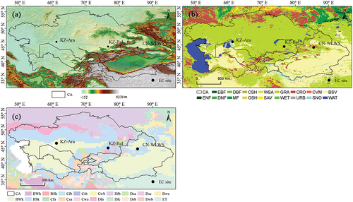
Central Asia (CA, 34.3°–55.4°N, 46.5°–96.4°E) is located in the middle of Eurasia and consists of the Xinjiang Province, China and five states: Kazakhstan, Kyrgyzstan, Tajikistan, Turkmenistan and Uzbekistan (Figure 1). The elevation gradually decreases from southeast to northwest and the terrain is dominated by plains and hills. The key climate feature is characterized by temperate continental climate, with cold winters and hot summers, scarce precipitation and large annual and daily temperature ranges (Han et al. 2016). The major land cover type includes grasslands and deserts and the foothills of the eastern mountainous area (of the study area) are covered by forests, alpine meadows and shrubs (Li et al. 2015). CA is characterized by a complex arid and semi-arid natural environment, which constitutes a fragile ecological area. In recent decades, the study area has experienced a complex and dramatic climate change, i.e. a rapid warming at a rate larger than the global average rate (Hu et al. 2014; Hoegh-Guldberg et al. 2018), more heat extremes (Reyer et al. 2017), some potential for a moderate rise in the occurrence of droughts (IPCC 2019) and an elevation of the CO₂ concentration in the atmosphere (Li et al. 2015).

Figure 1. (a) Digital Elevation Model (DEM) map from Global Land One-Kilometer Base Elevation, (b) Land-cover map of the IGBP classification schemes form MCD12Q1, (c) Köppen climate classification map form Climate Change and Infectious Diseases and eddy covariance site distribution in Central Asia (CA). The abbreviation refers to S2 in supplementary materials.

2.2 Data

2.2.1 Flux tower observations

In this study, three flux tower observations (Table 1) were used to evaluate the performance of the GPP products. These stations are not included in the flux network (i.e. FLUXNET (Pastorello et al. 2020)) and have thus not been utilized for the estimation and evaluation of the global GPP products. For each site, the data logger equipped in the EC system measured and recorded the carbon, water and energy fluxes at 2.0 m above ground at 10 Hz, as well as the ancillary measurements, including photosynthetically active radiation flux density, air temperature, humidity, precipitation, downward and upward shortwave and longwave radiation, soil temperature, soil moisture content, and soil heat flux and saved them as half-hourly averages. All measurements from the flux tower were carried out with data quality control and gap filling (Li et al. 2014). After achieving the gap filling, half-hourly NEE were obtained and further partitioned into ecosystem respiration (Reco) and GPP (Lasslop et al. 2010). The half-hourly GPP data were calculated as daily data and then the daily GPP were averaged to 8-day mean data to match the temporal resolution of the GPP products, covering the period from 30^th April to 18^th August 2012 at KZ-Ara site, from 23^rd May to 6^th September 2012 at KZ-Bal site and 1^st April to 1^st November in 2009, 2010, 2012 and 2013 at CN-WLWS site. Specifically, the tower-based GPP were only used to evaluate the 8-day GPP products due to the limited observation period.

Table 1. The information of the in-situ observations for the evaluation of the GPP products. AMT, annual mean temperature; AP, annual precipitation. KZ-Ara, Aral Sea station in Kazakhstan; KZ-Bal, Balkhash Lake station in Kazakhstan; CN-WLWU, Wulanwusu station in China.

Site	Longitude	Latitude	Vegetation type	AMT	AP	Time period	Reference
KZ-Ara	61.08°E	45.96°N	Shrub	8.3°C	140.5 mm	30^th April to 18^th August 2012	(Li et al. 2014).
KZ-Bal	76.63°E	44.57°N	Grass	5.7°C	140 mm	23^rd May to 6^th September 2012	(Li et al. 2014).
CN-WLWS	85.52°E	44.28°N	Crop	7.0°C	210 mm	1^st April to 1^st November in 2009, 2010, 2012 and 2013	(Ochege et al. 2022)

2.2.2 GPP products

Numerous mainstream ongoing GPP products are potential targets for our evaluation (Zhang et al. 2019). However, ten GPP products were finally selected after the synthetic consideration of the temporal coverage and resolution, spatio-temporal integrity, the requirements for the same units of the GPP, as well as the similarity in the original spatial resolutions. Basic information on these ten products used in this study is listed in Table 2.

Table 2. Information of ten Gross Primary Productivity (GPP) products. In the “GPP scheme” columns, LUE refers to the Light Use Efficiency, ML means Machine Learning, Proxies refers to the satellite-based direct proxies of the GPP and diagnostic means a diagnostic biophysical model. The spatial coverage of all ten products is global.

Name	GPP scheme	Temporal coverage	Temporal resolution	Spatial resolution	Validation	Reference
EC-LUE	LUE	1982 to 2017	8-d	0.05	95 EC sites (global)	(Zheng et al. 2020)
FLUXCOM	ML	2001 to 2015	8-d, monthly	0.083	224 EC sites (global)	(Jung et al. 2019)
FluxSat	LUE	1 March 2000 to 1 August 2020	daily	0.05	122 EC sites (global)	(Joiner et al. 2018)
GOSIF	Proxies	2000 to 2020	8-d, monthly, annual	0.05	91 EC sites (global)	(Li et al. 2019)
LUEopt	LUE	1 January 1982 to 1 January 2017	monthly	8 km	54 EC sites (global)	(Madani, Kimball, and Running 2017)
MODIS	LUE	2000 to present	8-d	1 km	Not performed	(Monteith 1972)
MuSyQ	LUE	1981 to 2018	8-d	0.05	126 EC sites (global)	(Wang et al. 2021)
NIRv	Proxies	1982 to 2018	monthly	0.05	104 EC sites (global)	(Wang et al. 2021)
PML	diagnostic	2002.07 to 2019.08	8-d	0.05	95 EC sites (global)	(Zhang et al. 2019)
VPM	LUE	2000 to 2016	8-d, monthly, annual	0.05	113 EC sites (global)	(Zhang et al. 2017)

The EC-LUE GPP product (Zheng et al. 2020) was generated by revising a LUE model which integrated the impacts of several environmental variables on GPP across a long-term temporal scale. This product performed well in simulating the spatial, seasonal, and interannual variations in global GPP (R² >0.5 at more than 95% validation sites).

The FLUXCOM GPP (Jung et al. 2019; Tramontana et al. 2016) product was produced by upscaling GPP estimates from FLUXNET EC towers with remote sensing (RS) and meteorological data (METEO) by ensemble means of various machine learning algorithms. This product contains two setups: (1) FLUXCOM RS uses high spatial resolution land surface biophysical parameters from Moderate-resolution Imaging Spectroradiometer (MODIS) observations as input for nine machine learning methods, while (2) FLUXCOM RS+METEO uses mean seasonal cycle of land surface variables with four global climate forcing data sets as input to three machine learning methods. As the proxy of FLUXNET observations, FLUXCOM products are often considered as a benchmark or reference in land-atmosphere interactions and global carbon and water cycle studies (Jiang and Ryu 2016; Jung et al. 2019). In this study, FLUXCOM RS was used because its GPP products have the finer spatiotemporal resolution than FLUXCOM RS+METEO.

The FluxSat GPP product (Joiner et al. 2018) was estimated by a simplified light use efficiency framework that uses only remote sensing data as inputs. This GPP product was shown to perform well or better than satellite data-driven products based on the validation results with FLUXNET 2015 GPP. The results also show that a large fraction of spatiotemporal variability in GPP across different plant functional types (PFTs) can be explained by using this satellite-based models.

The GOSIF GPP product (Li et al. 2019) was estimated using the global, OCO-2-based Solar-induced Chlorophyll Fluorescence (SIF) product (GOSIF) and linear relationships between SIF and GPP. Their modeled SIF showed a good performance across various biomes (R² = 0.79, root mean squared error (RMSE) = 0.07 W m⁻² µm⁻¹ sr⁻¹). The estimated GOSIF was highly correlated with GPP from 91 EC flux sites (R² = 0.73, p < 0.001) (Li et al. 2019; Qiu et al. 2020).

The LUEopt GPP product (Madani, Kimball, and Running 2017) was based on the well-known Monteith LUE equation but was improved by optimized LUE (LUEopt) values derived from selected FLUXNET sites. The overall accuracy of this GPP product (R² = 0.84, RMSE = 313 g C m⁻¹) showed a 15% R² and 34% RMSE improvement relative to baseline GPP simulations using LUEmax inputs.

The MOD17A2H GPP product was estimated based on the concept of the LUE (Monteith 1972). This study acquired the available MODIS GPP product in the Google Earth Engine (GEE) cloud-based platform (Gorelick et al. 2017) after identification and removal band-quality observations based on the quality assessment/quality control (QA/QC) band. We applied the scale factor of 0.0001 to each MOD17A2H pixel to translate the numerical value into the sequestered carbon value (Running, Qiaozhen, and Zhao 2015).

The MuSyQ GPP product (Wang et al. 2021) was generalized using the improved MuSyQ algorithm which was derived from a LUE model. The accuracy of this product was slightly higher than that of the MOD17 GPP product when compared with the FLUXNET GPP.

The NIRv GPP product (Wang et al. 2021) was estimated using a simple linear regression to establish the relationship between satellite-based near-infrared reflectance (NIRv) and GPP. Grayson et al (Badgley, Field, and Berry 2017) first proposed the quantification method of NIRv, and found that the NIRv have strong correlations with SIF, site-level and globally gridded estimates of GPP. Thus, the NIRv can be considered as one direct proxy of GPP. This product could accurately represent both the monthly and annual GPP variations across 104 EC sites and the global performance fell between the estimations from machine learning (ML), LUE, and processed-based modes.

The PML GPP product (Zhang et al. 2019) was generated from MODIS data together with Global Land Data Assimilation System (GLDAS) meteorological forcing data using a coupled diagnostic biophysical model (called PML-V2) that, built using GEE (https://data.tpdc.ac.cn/en/). This product showed robust model performance (RMSE = 2.13 g C m⁻² d⁻¹ and bias = 3.3%) based on the cross-validation at 95 widely-distributed flux towers for 10 plant functional types.

The VPM GPP product (Zhang et al. 2017) was estimated by vegetation photosynthesis model (VPM) algorithm, which used an improved LUE theory that overcomes the limitation of MOD17. The overall accuracy of the VPM GPP dataset is relatively high with an R² of 0.74 and a low RMSE of 2.08 g C m⁻² d⁻¹.

2.2.3 Ancillary data

The explanatory variables have been used for the attribution analysis and were all averaged to mean values during the period 2003–2015 to match the related uncertainties of the GPP products. These explanatory variables described the land surface biophysical parameters, climate and terrain information of the study area. We used the following four MODIS data products: the MOD13A2 including the normalized difference vegetation index (NDVI) (Huete et al. 2002) and enhanced vegetation index (EVI) (Huete et al. 1997), MOD11A2 including the daytime and nighttime land surface temperature (LSTd and LSTn) (Wan 2008) and MOD15A2 including the leaf area index (LAI) and fraction of absorbed photosynthetic active radiation (FPAR) (Myneni et al. 2002) and MCD12Q1 land cover (LC) data (Friedl et al. 2010). The near-ground meteorological variables were extracted from the ECMWF Reanalysis v5 - Land (ERA5-Land) data (Muñoz-Sabater et al. 2021), including the temperature (Tm), total precipitation (P), Surface downwelling shortwave radiation (RSDN), layer 1 (0–7 cm depth) soil moisture as the near-surface soil moisture (SM1) and the mean of layers 2 (7–28 cm) and 3 (28–100 cm) as the sub-surface soil moisture (SM2). The climate zones (CZs) were derived from the Köppen-Geiger world maps’ climate classification (http://koeppen-geiger.vu-wien.ac.at/). The Global Land One-Kilometer Base Elevation (GLOBE, (Hastings et al. 2002)) provided the digital elevation model (DEM). The aspect and slope data were further obtained from the DEM data. In addition, the effect of the sample size on the TCH-based relative uncertainties’ (RU) estimates of the GPP products should be considered and also added to the attribution model as explanatory variables (Liu et al. 2021).

For each MODIS product, the low quality pixels were removed by using the quality assessment/quality control (QA/QC) flags (Zhang et al. 2021). The land cover data which comprise the International Geosphere-Biosphere Programme (IGBP) classification scheme were selected. The preprocessing MODIS and ERA5-Land data were conducted in the GEE platform (Gorelick et al. 2017).

2.3 Methods

2.3.1 Data preprocessing

Ten GPP products with a different spatio-temporal resolution and format were preprocessed to obtain a comparable and uniform specification (Figure 2). The preprocessing steps are as follows:

1. Unit unification. The products in the units of the monthly GPP product (g C m⁻² m⁻¹) from GOSIF and VPM were converted into monthly mean values in the units of g C m⁻² d⁻¹ for subsequent evaluation. The cumulative composites of the GPP values were converted into 8-day mean values in the units of g C m⁻² d⁻¹ for a subsequent evaluation.

2. Temporal aggregation. The 8-d mean GPP (i.e. MODIS, PML, EC-LUE) and the monthly mean GPP (i.e. FLUXCOM, LUEopt, NIRv) were aggregated into the annual values of the corresponding products, respectively. The daily FluxSat were aggregated into 8-day mean, monthly mean and annual values, respectively.

3. Spatial aggregation. The nearest-neighbor interpolation was used to resample the FLUXCOM, MODIS and LUEopt GPP products and ancillary datasets to the spatial resolution of 0.05°×0.05°.

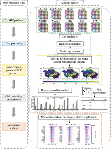
Figure 2. The framework for evaluating GPP products in areas lacking observation data.

The overlapping time span of the ten GPP products from 2003 to 2015 have been used in the intercomparison. Except for the LUEopt and NIRv, all remaining products were used in an 8-day time step comparison. Except for the MODIS, PML and EC-LUE, all remaining products were utilized in the monthly time step comparison. All of the ten products were selected for a yearly comparison.

2.3.2 Theil-Sen median analysis and the Mann – Kendall trend test

The combination of the Theil-Sen median trend analysis (Sen 1968) and Mann-Kendall test (Forthofer and Lehnen 1981) was applied to detect the change trends in the long-term time series’ GPP data. The Theil-Sen median trend analysis is a robust non-parametric statistical method. The Mann-Kendall is a non-parametric statistical test to determine the trend significance. In this research, the results of the Theil-Sen median trend analysis and Mann-Kendall test were categorized into 3 classes (i.e. significant decrease, significant increase and no significant change trend) according to the criteria in the Supplementary material S3.

2.3.3 GPP uncertainty quantification method

For each site-scale GPP estimation, the coefficient of determination (R²), the root-mean-square error (RMSE) and the mean absolute error (MAE) were used to evaluate the performance of the 8-day GPP products against the flux tower-based GPP observations during the period of limited flux observations. For the spatial-scale GPP values, the three-cornered hat (TCH) method was adopted. The theory of TCH was developed by (Gray and Allan 1974) and (Tavella and Premoli 1994). TCH could be employed to evaluate the relative uncertainties among the ten GPP products at a regional scale without any prior knowledge. It allows at least three different product time series to participate in the calculation simultaneously, with tolerance to the error cross-correlation to a certain extent. The details of the TCH are described in the Supplementary material S3.

2.3.4 Attribution analysis

Fully understanding the relationship between the underlying surface factors, near surface meteorological factors and GPP product uncertainty can play a significant role in finding the source of the GPP uncertainty and to improve the performance of the GPP model. Firstly, we trained the XGBoost model and then applied the Shapley additive explanation (SHAP) in order to separate the marginal contribution of each predictor to the target variable.

XGBoost stands for the Extreme Gradient Boosting (XGB) algorithm (Chen and Guestrin 2016), which is an implementation of the Gradient Boosted decision trees (GBDT). GBDT is an addition model based on the Boosting integration idea, which utilizes a forward distribution algorithm for greedy learning in training. XGB possesses the characteristics of high efficiency, flexibility and portability and is widely used by data scientists so as to achieve a better performance on many ML challenges. For each RU of the GPP product, we treated the RU as the target variable and the corresponding driven factors as predictors by a common hyperparameters’ setting optimized by the pixel-level dataset (learning rate: 0.8, max depth: 13, number of estimators: 50). Our results show that the performance of XGboost is reliable (Supplementary material Table S6.1).

SHAP (Lundberg and Lee 2017) is a game theoretic approach to explain the output of any ML model and its core concept is Shapley value. By constructing an additive interpretation model, SHAP considers all features as “contributors” and generates a prediction value for each prediction sample. Shapley value is the value assigned to each feature in the sample (i.e. marginal contribution). Therefore, the SHAP model might be coupled with any ML model so as to explain the contribution of each sample and feature to the corresponding predicted value. For each trained model, we applied the SHAP dependence method to isolate the marginal contributions of each single factor to the GPP RU (Supplementary material S7) and then, we ranked the variable importance by SHAP importance algorithm (absolute weighted averaged marginal contributions from each predictor variable).

3 Results

3.1 Inter-comparison of the spatio-temporal patterns of GPPs at different time scales

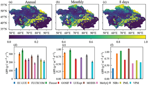
Here, the variance was used to quantify the spatial distribution difference among ten GPP products. At various time scales, the spatial distribution difference of the GPP products in CA showed similar patterns while the values seem quite different (Figure 3). The regions with high variance values were distributed along the Tianshan Mountains and the northern part of the study area and these regions also demonstrated higher GPP values (Fig S4. 1 to Fig S4. 3). The areas with low variance values were located in the southwest and southeast regions due to the lower GPP (close to 0) values. The maximum GPP values were noticed in Fluxsat with a value of 340.69 g C m⁻² y⁻¹, 0.93 g C m⁻² d⁻¹ and 0.93 g C m⁻² d⁻¹ for the mean annual, monthly and 8-day GPP values, respectively. The minimum GPP occurred in the EC-LUE (124.26 g C m⁻² y⁻¹), VPM (0.56 g C m⁻² d⁻¹) and EC-LUE (0.34 g C m⁻² d⁻¹) for the mean annual, monthly and 8-day GPP values, respectively. Furthermore, the annual, monthly and 8-day GPP values showed inconsistency regarding different land cover types and climate zones (Table S4.1 to S4. 3). In terms of land cover types, the maximum GPP values of EC-LUE, FLUXCOM, MODIS and MuSyQ occurred in ENF, MF, DBF and MF, respectively, while the Fluxsat, GOSIF, LUEopt, PML and VPM are in the CSH. In term of climate types, the maximum GPP values for all 10 products occurred in Dwb, but the next values did not show the consistent change relationship. Similar results were also found in the mean monthly values and mean 8 days GPP values.

Figure 3. The spatial distribution difference and comparison of (a) (d) mean annual, (b) (e) mean monthly and (c) (f) mean 8-day GPP in CA from 2003 to 2015. The spatial distribution difference between the ten GPP products was quantified at a pixel level by calculating the variance. For the (d) (e) and (f), the error bars indicate a ± 1 standard deviation.

At different time scales, the temporal variations of various GPP products in CA were similar but the magnitude was completely different (Fig S4. 4). For the interannual GPP values, the overall fluctuation tendency was similar, but varies greatly for different land cover types or climate zones (Fig S4. 5). For the monthly and 8-day GPP values, the temporal variations of different GPP products indicated a reverse U-shaped pattern but the timing of the peak values was inconsistent among the different land cover types or climate zones (Fig S4. 6 and Fig S4. 7).

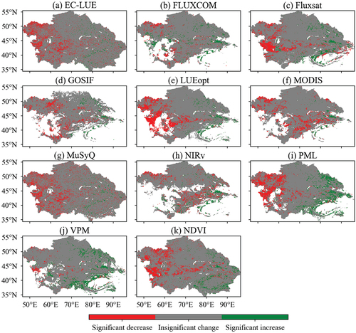
Here, we used the NDVI to represent the change trend of the vegetation, which can be used to evaluate the change trend of ten GPP products (Figure 4 k). The areas of significant decrease of the NDVI (mainly located in the eastern and central regions) were obviously larger than the areas of significant increase (located in the western regions). Although all GPP products showed a variation pattern of increase in the east and a decrease in the west, the spatial distribution was varied for the NDVI. The spatial variation of Fluxsat, GOSIF, LUEopt, MODIS, NIRv and PML was consistent with the vegetation change but the NIRv show more data gap areas. The distribution of the significant increase areas in EC-LUE and MuSyQ was more fragmented than the areas of increased vegetation. The FLUXCOM showed a significant increase area in the west, which was not consistent with the vegetation change. Although the VPM demonstrated a similar spatial variation pattern for the vegetation, the areas of significant increase were obviously larger than the areas with a significant decrease.

Figure 4. Spatial distributions of the change trends of ten GPP products (a – j) and NDVI (k) in CA from 2003 to 2015. The different trends are indicated by different colors: red pixels for a significant decrease, green pixels for a significant increase and gray pixels for no significant change (p < 0.05).

3.2 Relative uncertainties’ (RU) quantification of GPP products at different time scales

3.2.1 GPP validation with flux tower observations

In general, all eight GPP products performed differently in predicting the GPP, with R², RMSE and MAE ranging between 0.34 and 0.76, 1.87 and 2.64 g C m⁻² d⁻¹ and 1.07 and 1.49 g C m⁻² d⁻¹, respectively. The FLUXCOM products have the highest R² value and a relatively low RMSE and MAE (Table 3). For the individual site, all eight GPP products also performed differently predicting the GPP (Table S5. 1). The FLUXCOM showed a better performance at the KZ-Ara and KZ-Bal site with higher R² values and lower RMSE and MAE values. The EC-LUE and MuSyQ denoted higher R² values and lower RMSE and AME values at the CN-WLWS site.

Table 3. Comparison of the 8-day GPP products against the in-situ observations. The unit (of the RMSE and MAE) is g C m⁻² d⁻¹.

	EC-LUE	FLUXCOM	Fluxsat	GOSIF	MODIS	MuSyQ	PML	VPM
R^2	0.46	0.76	0.7	0.66	0.63	0.58	0.34	0.63
RMSE	2.29	1.88	1.87	2.27	2.15	1.95	2.64	2.11
MAE	1.23	1.15	1.11	1.38	1.23	1.07	1.49	1.32

3.2.2 Relative uncertainties’ quantification of the GPP products with the TCH method

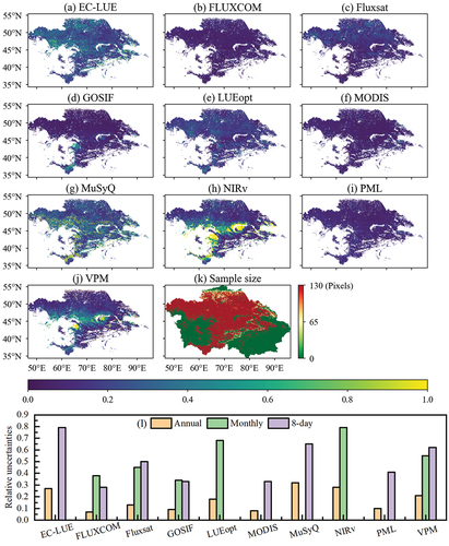
The RU of the GPP varied depending on the difference in products, time scales and land cover types or climate zones (Table S5.2 – S5.4). For the annual GPP products (Figure 5), the lower RU occurred in the north and south of CA, while the higher RU occurred in the middle of CA. The monthly and 8-day GPP products generated a higher RU (0.34–0.79, 0.28–0.79, respectively) than the corresponding yearly GPP products (0.07–0.32) across whole CA (Figure 5 l) but the distribution was consistent with the yearly GPP (Fig S5.1 and Fig S5.2). The FLUXCOM, Fluxsat, GOSIF, MODIS and PML showed a similar spatial RU pattern and had a lower RU in most areas of CA, while the NIRv and VPM denoted a similar pattern with a significant higher RU in the middle part of CA. The RU of MuSyQ increased from the north to the south part. The GPP products tend to generate a larger RU in the middle part of CA due to a low GPP magnitude. Over the surface of CA, the sample size decreased from the center to the margins. Moreover, the distribution of bare land in the southeast and southwest of CA induced no pixels were involved in the RU calculation and generated the low GPP magnitude (e.g. EC-LUE, GOSIF, MuSyQ, PML and VPM) or even no valid pixels (FLUXCOM, Fluxsat, LUEopt, MODIS and NIRv). In general, the FLUXCOM performed best among the yearly and 8-day GPP products with a low RU of 0.07 and 0.28, while the monthly GOSIF did best with a RU of about 0.34.

Figure 5. (a) – (j) the relative uncertainties of the annual GPP products in CA and (k) the sample size used in TCH. (l) the relative uncertainties of the GPP products at different time scales in CA by means of the TCH method (2003–2015).

4 Discussion

4.1 Comparison of the TCH-derived uncertainty and RMSE

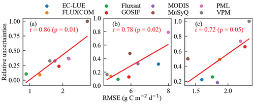
The performance of the TCH method could be evaluated by the RMSE because both have the same calculation formula as Eq (14) in the Supplementary material. The evaluation of the TCH results was only conducted at EC sites at an 8-day time scale due to the limited observation period. We detected a good agreement in the relationship between the RU and RMSE values, even in the cases of a limited number of EC stations and observation periods (Figure 6). The highest Pearson Correlation Coefficient (r) value was noticed at the KZ-Ara and lowest at the CN-WLWS site, which may be caused by farmland management activities, such as drip irrigation and plastic mulching (Yuan et al. 2019). The good agreement between the TCH results and RMSE at the EC site scale indicates that the overall TCH-based relative uncertainty results are quite reasonable for the entire CA region.

Figure 6. Comparison of the TCH-derived relative uncertainties (y-axis) and RMSE (x-axis) for the 8-day GPP products at the (a) KZ-Ara, (b) KZ-Bal and (c) CN-WLWS. The red lines demonstrate the regression line.

4.2 Attribution of the relative uncertainties of the GPP products

Different GPP models lead to various simulation uncertainties. In general, the FLUXCOM outperformed other models for the GPP estimation because it makes full use of the FLUXNET global dataset and ensemble the output of multiple ML models so as to generate more reliable GPP products in CA.

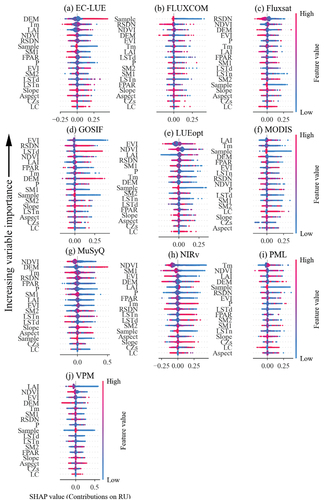
In addition, the vegetation, energy, water, climate and terrain factors are essential for an accurate estimation of the regional GPP. Investigating the impact of these factors on the RU of the GPP might provide a theoretical foundation to understand the RU source. Here, we applied the XGBoost and SHAP attribution method in order to detect the relative importance of different factors to the RU at a different time scale and how these impact the RU of GPP products (Figure 7, and Fig S7.1 – Fig S7. 2). Some factors such as the NDVI, DEM, LAI, RSDN and Tm have a higher contribution than other factors to the RU of GPP products on different time scales. However, these factors affect the RU in different ways and for various GPP products. The possible reason is that these factors have obvious positive or negative effects on the growth of vegetation. Specifically, we see that larger NDVI values are associated with smaller SHAP values in most of the LUE models (i.e. EC-LUE, LUEopt, MODIS, MuSyQ and VPM) and two Proxies models indicating these models simulates GPP better in high NDVI values regions. The NDVI values have no clear relationship with the RU of the annual FLUXCOM GPP but show a positive contribution at the monthly and 8-day scales. It indicates that the FLUXCOM had a lower performance when estimating the real GPP values in the areas with high NDVI values. The possible reason is that LUE and Proxies models only used vegetation-related input data to estimate GPP, while ML and diagnostic models used more water and energy-related input data except vegetation, which may weaken the impact of vegetation characteristics on ML and diagnostic GPP uncertainty. In addition, the spatial heterogeneity of dryland also may cause vegetation to play different or even opposite roles in different GPP estimation models (Barnes et al. 2021). For the DEM, the RU of three LUE models (Fluxsat, MODIS and VPM) and one Proxies model (NIRv) decreased depending on the increasing elevation, while the higher DEM values will augment the RU of the EC-LUE, GOSIF and MuSyQ. In terms of LAI, a high LAI could only reduce the RU of the VPM products, while there is no clear relationship between the LAI and RU of the other GPP products. The possible reason is that the impact of LAI on RU is weakened due to the existence of NDVI, both of which are indicators of regional vegetation characteristics. For the FLUXCOM, Fluxsat, MuSyQ and NIRv, the higher RSDN values will lower the RU values. Although the Tm contributes significantly to the RU of most annual GPP products, there was no obvious connection between the Tm and SHAP value. The higher the Tm, the greater the SHAP value of RU in LUEopt, EC-LUE, Fluxsta, MODIS, MuSyQ, PML and VPM. Some factors, such as the EVI, FPAR, Sample, SM1, SM2, LSTd, LSTn and P, have a lower contribution than the above-mentioned factors and their relative importance changes with the different time scales. The remaining factors such as the LC, CZs, Aspect and Slope contributed less to the RU of the GPP products at different time scales. The above-mentioned information offers a quantitative understanding of the RU of different GPP products and practical directions for the model improvements. It would be meaningful to discuss why each environmental characteristic had a significant effect on RU, in connection with regional characteristics. However, the purpose of this paper is to provide potential users of GPP products in CA with a quick selection of GPP products and a general understanding of their uncertainty. It is obvious that more detailed data and reasonable control experiments are needed to explore the deeper reasons for the impact of environmental characteristic on RU.

Figure 7. Relative importance and marginal contribution (SHAP values) of multiple variables to the relative uncertainties of the annual GPP products. The x axis represents the SHAP value, and its value >0 indicates that the explanatory variable will increase the RU of the GPP and vice versa. The color stands for the feature value (red: high, blue: low).

Furthermore, we summarized the main input of all GPP products so as to investigate the source of the RU in the GPP from a qualitative perspective (Table S7.1 in the supplementary material). In agreement with our expectations, all GPP models included more vegetation-related information. Most of the LUE models (i.e. EC-LUE, Fluxsat, MuSyQ and VPM) and the NIRv GPP products only comprise one or lack the energy and water available inputs, which may result in high RU compared with ML model and other products over CA. It has been found that water stress limits the LUE and dominates the interannual variation productivity, which constitute the main influencing factor for the LUE (Barman, Jain, and Liang 2014; Xie et al. 2020). In recent years, extreme events (such as droughts) have occur frequently, and has a profound impact on the growth of the vegetation, which finally contribute to the increase in the uncertainty of terrestrial ecosystem productivity (Pei et al. 2020). The vapor pressure deficit (VPD) and soil moisture (SM) are the two main drivers for drought stress on vegetation (Liu et al. 2020). According to Table S7. 1, only the LUEopt model considered the VPD and SM as available water input variables, which may reduce the RU comparison with other LUE models (e.g. EC-LUE and MuSyQ) to some extent. Since the FLUXCOM lacks the SM information as model input, they used the normalized difference water index and land surface water index (LSWI) as an alternative SM input indicator, which may result in a low RU. Previous studies showed that the water stress factors that reflect the physiological and ecological characteristics of the vegetation (such as the LSWI) rather than atmospheric water (such as VPD) or other meteorological substitutes should be considered when applying the GPP models in drought conditions (Pei et al. 2020). Among the LUE models and the improvements, the EC-LUE and VPM include the C4% (and only the EC-LUE considered the CO₂ fertilization effect on the GPP). However, these additional factors do not seem to reduce the RU of these products in the CA region. The possible reason might be that the determination of the LUEmax depends on the look-up table (Wei et al. 2017). Even for some improved LUE models (i.e. LUEopt), the LUE is determined according to the global flux tower (Madani, Kimball, and Running 2017) but the lack of EC observations in CA may still highlight this issue. The Proxies model that upscale the SIF-GPP relationship at EC site to the global scale for obtaining the GPP products also has similar problems due to the lack of EC site in CA. In addition, the vegetation in drylands is more sensitive to the changes in the environmental factors, which could lead to a significant underestimation of the LUEmax in the drylands ecosystems (Wang et al. 2019). Thus, the lack of suitable LUE parameters in drylands and the inability to accurately simulate the complex relationship between the water and LUE are the main reasons why the performance of most LUE models is lower than the one of FLUXCOM or GOSIF in CA. The effective ways to improve the performance of the LUE models applied to CA are to comprise the construction of EC flux towers in appropriate points of arid areas and to consider the water-related variables (e.g. SM, VPD or LSWI) as input for the LUE model parameterizations. In general, the FLUXCOM includes most of the vegetation, water and energy information required for the GPP estimation, especially key information (i.e. LSWI) under drought conditions, which makes the performance better than other products. There is a fact to be acknowledged that describe the problems in CA that arise due to the limitations of each GPP product, which is more important than the input parameters. But the lack of adequate EC observations data makes it impossible to carry out more experiments to deepen our discussion. Future studies should select the dryland with sufficient EC sites to investigate the RU of each GPP product.

The model input dataset errors and scale mismatch between the input and output also affected the RU of the GPP products. The input dataset covers the tower-based observations, meteorological observations or reanalysis data and remote sensing data. The EC data collection process will be influenced by systematic and random errors (Fratini et al. 2018). The errors in the grid-level data (such as meteorological reanalysis data and remote sensing data) were derived from the spatial heterogeneity, inconsistent sensors and the inversion method. In terms of the commonly used data such as MODIS products, the global relative uncertainty (associated with the MODIS LAI) is 26.6%, while the MODIS-LST measures about 4.5 K (Zhang et al. 2021). Previous study also found that the uncertainty of GPP is mainly due to the meteorological reanalysis data (Tramontana et al. 2015). In addition, mistakes will also be found in the GPP estimation when regridding the coarse resolution model input data to fine resolution model output data. For example, the spatial resolution of the model input data, such as the MERRA-2 (0.625∘ in longitude by 0.5∘ in latitude) and NCEP-reanalysis II (~1.875°×2°), was coarser than the model output (0.05°×0.05°). Errors in the model input may degrade the model performance to capture the correct relation between the GPP and the drivers and finally trigger the high RU of the GPP.

The model validation also has a significant impact on the RU of the GPP products (Table 2). FLUXCOM has been trained and validated with global 224 EC sites. However, the RU of the annual FLUXCOM was less than the monthly and 8-day RU. This is because of the fact that the global flux station covers various vegetation types but cannot cover the full arid areas. This indicates that the availability of the EC sites in CA may be limited to an annual scale, nevertheless attention should be paid to it on a higher time scale.

4.3 Limitations and implications for future model improvements

Despite the comprehensive evaluation of ten GPP products in CA conducted in this study, using the EC observations and the TCH method, we recognize that our evaluation still contains some limitations. There are several sources of uncertainties associated with our GPP evaluation, including: (1) limited observation sites: Three EC sites with homogeneous underlying surfaces are sparsely distributed and provided for only growing season observations to evaluate the 8-day GPP products. In addition, the EC measurements are site-scale observations and only represents the fluxes from the tower footprint up to several square kilometers (Göckede et al. 2008), but the spatial resolution of the GPP products measured from 1 km to 10 km. Therefore, it is hard to evaluate the GPP products with EC observations for different time scales and conditions. (2) Sample size in TCH: For these ten GPP products, the uncertainty variation and the difference of the corresponding determinants are mainly caused by the errors of the GPP algorithms or models and some of these are introduced by the uncertainty of the evaluation methods. The sample size is a possible source of uncertainty for the TCH method. For a pixel in the GPP products, the minimum number of samples of a given time series may affect the stability of uncertain results (Xu et al. 2019; Liu et al. 2021). Thus, the sample size is used as an explanatory variable in the attribution method so as to calibrate the contribution of other explanatory variables in the attribution analysis. (3) Preprocessing GPP products and explanatory variables: In order to conduct the TCH method and attribution analysis, the GPP products and explanatory variables were resampled to 0.05 ° × 0.05°. Although efforts have been made to select the products with a similar spatial resolution, however, some uncertainties were still introduced in this work caused by the resampling treatment (Wang, Wang et al. 2021). In addition, we used the ancillary data without evaluating their applicability in CA, which may also lead to some uncertainties in our results. However, this lies beyond the scope of this study. These data were only applied to deliver some general cognition for the RU of the GPP products.

The dryland ecosystems are more sensitive to climate change, which makes vegetation more vulnerable to changes in environmental factors, affecting the parameters of the model quite differently from other regions. Our results indicate that the FLUXCOM have a better performance than other products on the annual scale, while its performance is still unsatisfactory on the monthly and 8-day scales. The FLUXCOM variation presents some inconsistencies in vegetation change in CA and could not estimate the monthly and 8-day GPP very well, especially for high NDVI values. Thus, to improve the performance of the FLUXCOM model in arid regions, we should not only consider the EC sites in CA during the model training, but also incorporated the special physiological and ecological processes scheme to capture the characteristics of drylands vegetation in the model. For the LUE models, an attribution analysis shows that the performance of the LUE model is generally low because the LUE parameters are not suitable for the special physiological and ecological vegetation processes in the arid areas and there is also a lack of water-related available variables in the LUE models. For the Proxies models, the RU of the NIRv is obviously higher than the GOSIF. The attribution analysis indicates that the energy (e.g. Tm and PAR) and water (e.g. soil moisture) related variables are strongly affecting the RU of the NIRv in addition to the vegetation index related variables. Thus, the lacking variables (such as soil moisture and radiation) may be the main trigger for the high RU of the NIRv products. For the diagnostic model, the PML products seem to maintain a high RU in the GPP estimations. The high RU of the PML correlated with high DEM values, which are not used as input for the PML model. Hence, it is noted that we could obtain a higher performance of the PML GPP estimation when considering the influence of the elevation.

Theoretically, the feature importance and SHAP value of the explanatory variables could reflect the contribution of the driving factors to RU, which is very instructive to improve the algorithm and the models. Specifically, if the driver is also an input variable in the model and the greater the importance of the driver, it implies that the lower the correlation between this variable and the GPP product. It may be necessary to improve the module related to the variable. An example that matches this explanation is the NDVI related module in FLUXCOM. Otherwise, if the explanatory variable is not an input variable of the model but its contribution to the relative uncertainty is greater than for other variables, it may indicate that the consideration of this variable in the model might reduce the product uncertainty. The lack of DEM as input of the PML model is the example for this explanation. Our study offers the comprehensive evaluation of ten GPP products and investigate their sources of uncertainty in CA. These results will help us to better understand the applicability of various GPP products in CA and are expected to help us recognize the advantages and disadvantages of different technologies for estimating the GPP and their complementarity. Furthermore, the RU of each product derived from the TCH method is also valuable for improving the GPP estimation. We could apply the uncertainty information obtained from other products to make a better use of FLUXCOM or use it in a combined product, e.g. a weighted combination of the different products (Xu et al. 2020; Zhang and Aizhong 2022).

5 Conclusions

This study aims to comprehensively evaluate ten GPP products (i.e. EC-LUE, FLUXCOM, Fluxsat, GOSIF, LUEopt, MODIS, MuSyQ, NIRv, PML and VPM) of four types (i.e. LUE, ML, Proxies, diagnostic) on a multi- temporal scale in Central Asia (CA). The tower-based observations from three EC sites were used to validate these products and the three-corned hat (TCH) method was utilized to quantify the uncertainties of these GPP products in whole CA. Finally, an attribution analysis was performed to explore the characteristics and drivers of the variations of relative uncertainty for these ten GPP products at different time scale. Our results could be summarized as follows:

1. The regions with high variance values were distributed along the Tianshan Mountains and the northern part of the study area and these regions also showed higher GPP values. The spatial variation of Fluxsat, GOSIF, LUEopt, MODIS, NIRv and PML were consistent with the vegetation change.

2. According to the EC observations and TCH results, the FLUXCOM showed smaller relative uncertainties than the other products at different time scales.

3. According to the attribution analysis, different products corresponded to different sources of uncertainty. Taking the EC site located in CA into account as input data for the model training is a general method to improve the accuracy of these models. In addition, the ML model could incorporate the special physiological and ecological processes of vegetation in drylands for improving the precision of the GPP estimation in CA. Regarding the LUE models, tuning the suitable LUE parameters for the dryland ecosystems and considering the available water-related (e.g. SM, VPD or LSWI) could be two main paths to improve the performance of the LUE model in CA. For the Proxies model, the missing variables (such as soil moisture and radiation) may be the main reason for a high RU of the Proxies products. By considering the DEM variable as input data, the performance of the PML in CA might be improved for the diagnostic model.

Acknowledgments

We thank the Research Center for Ecology and Environment of Central Asia，Chinese Academy of Sciences for the support of data for this study.

Disclosure statement

No potential conflict of interest was reported by the authors.

Data availability statement

The data that support the findings of this study (i.e. the TCH results of ten GPP products) are available at figshare (https://doi.org/10.6084/m9.figshare.21505017.v2).

Additional information

Funding

 This work was supported by the Strategic Priority Research Program of the Chinese Academy of Sciences (Grant No. XDA20060302), the Tianshan Talent Cultivation (Grant No. 2022TSYCLJ0001), the High-End Foreign Experts Project, the Natural Science Foundation of Sichuan (Grant No. 2022NSFCSC1124), and the National Natural Science Foundation of China (42205127).

References

- Ahlström, A., R. Raupach Michael, G. Schurgers, B. Smith, A. Arneth, M. Jung, M. Reichstein, et al. 2015. “The Dominant Role of Semi-Arid Ecosystems in the Trend and Variability of the Land CO2 Sink.” Science 348 (6237): 895–20. doi:10.1126/science.aaa1668.
- Badgley, G., C. B. Field, and J. A. Berry. 2017. “Canopy Near-Infrared Reflectance and Terrestrial Photosynthesis.” Science Advances 3 (3): e1602244. doi:10.1126/sciadv.1602244.
- Baldocchi, D. D. 2003. “Assessing the Eddy Covariance Technique for Evaluating Carbon Dioxide Exchange Rates of Ecosystems: Past, Present and Future.” Global Change Biology 9 (4): 479–492. doi:10.1046/j.1365-2486.2003.00629.x.
- Barman, R., A. K. Jain, and M. Liang. 2014. “Climate-Driven Uncertainties in Modeling Terrestrial Gross Primary Production: A Site Level to Global-Scale Analysis.” Global Change Biology 20 (5): 1394–1411. doi:10.1111/gcb.12474.
- Barnes, M. L., M. M. Farella, R. L. Scott, D. J. P. Moore, G. E. Ponce-Campos, J. A. Biederman, N. MacBean, M. E. Litvak, and D. D. Breshears. 2021. “Improved Dryland Carbon Flux Predictions with Explicit Consideration of Water-Carbon Coupling.” Communications Earth & Environment 2 (1): 248. doi:10.1038/s43247-021-00308-2.
- Bi, W., W. He, Y. Zhou, W. Ju, Y. Liu, Y. Liu, X. Zhang, X. Wei, and N. Cheng. 2022. “A Global 0.05 Degrees Dataset for Gross Primary Production of Sunlit and Shaded Vegetation Canopies from 1992 to 2020.” Scientific Data 9 (1): 213. doi:10.1038/s41597-022-01309-2.
- Chen, T., and C. Guestrin. 2016. “XGBoost: A Scalable Tree Boosting System.” In KDD ’16: The 22nd ACM SIGKDD International Conference on Knowledge Discovery and Data Mining, 785–794. San Francisco California USA: Association for Computing Machinery.
- Forthofer, R. N., and R. G. Lehnen. 1981. “Rank Correlation Methods.” In Public Program Analysis: A New Categorical Data Approach, edited by R. N. Forthofer and R. G. Lehnen, 146–163. Boston, MA: Springer US.
- Fratini, G., S. Sabbatini, K. Ediger, B. Riensche, G. Burba, G. Nicolini, D. Vitale, and D. Papale. 2018. “Eddy Covariance Flux Errors Due to Random and Systematic Timing Errors During Data Acquisition.” Biogeosciences 15 (17): 5473–5487. doi:10.5194/bg-15-5473-2018.
- Friedl, M. A., D. Sulla-Menashe, B. Tan, A. Schneider, N. Ramankutty, A. Sibley, and X. Huang. 2010. “MODIS Collection 5 Global Land Cover: Algorithm Refinements and Characterization of New Datasets.” Remote Sensing of Environment 114 (1): 168–182. doi:10.1016/j.rse.2009.08.016.
- Göckede, M., T. Foken, M. Aubinet, M. Aurela, J. Banza, C. Bernhofer, J. M. Bonnefond, et al. 2008. “Quality Control of CarboEurope Flux Data – Part 1: Coupling Footprint Analyses with Flux Data Quality Assessment to Evaluate Sites in Forest Ecosystems.” Biogeosciences 5 (2): 433–450. doi:10.5194/bg-5-433-2008.
- Gorelick, N., M. Hancher, M. Dixon, S. Ilyushchenko, D. Thau, and R. Moore. 2017. “Google Earth Engine: Planetary-Scale Geospatial Analysis for Everyone.” Remote Sensing of Environment 202: 18–27. doi:10.1016/j.rse.2017.06.031.
- Gray, J. E., and D. W. Allan. 1974. A Method for Estimating the Frequency Stability of an Individual Oscillator. Paper presented at the 28th Annual Symposium on Frequency Control, 29-31 May 1974, Atlantic City, NJ, USA.
- Han, Q., G. Luo, L. Chaofan, A. Shakir, W. Miao, and A. Saidov. 2016. “Simulated Grazing Effects on Carbon Emission in Central Asia.” Agricultural and Forest Meteorology 216: 203–214. doi:10.1016/j.agrformet.2015.10.007.
- Hastings, D. A., P. K. Dunbar, G. M. Elphingstone, M. Bootz, H. Murakami, P. Holland, N. A. Bryant, et al. 2002. “SAFARI 2000 Digital Elevation Model, 1-km (GLOBE).” In ORNL Distributed Active Archive Center.
- Hoegh-Guldberg, O., D. Jacob, M. Bindi, S. Brown, I. Camilloni, A. Diedhiou, R. Djalante, et al. 2018. “Impacts of 1.5¡ãc Global Warming on Natural and Human Systems.” In Global Warming of 1.5¡ãc, edited by V. Masson-Delmotte, P. Zhai, H. O. P?rtner, D. Roberts, J. Skea, P. R. Shukla, and A. Pirani, 175–311. UK and New York, NY, USA: IPCC Secretariat.
- Houghton, R. A., E. A. Davidson, and G. M. Woodwell. 1998. “Missing Sinks, Feedbacks, and Understanding the Role of Terrestrial Ecosystems in the Global Carbon Balance.” Global Biogeochemical Cycles 12 (1): 25–34. doi:10.1029/97GB02729.
- Huete, A., K. Didan, T. Miura, E. P. Rodriguez, X. Gao, and L. G. Ferreira. 2002. “Overview of the Radiometric and Biophysical Performance of the MODIS Vegetation Indices.” Remote Sensing of Environment 83 (1): 195–213. doi:10.1016/S0034-4257(02)00096-2.
- Huete, A. R., H. Q. Liu, K. Batchily, and W. van Leeuwen. 1997. “A Comparison of Vegetation Indices Over a Global Set of TM Images for EOS-MODIS.” Remote Sensing of Environment 59 (3): 440–451. doi:10.1016/S0034-4257(96)00112-5.
- Hu, Z., C. Zhang, Q. Hu, and H. Tian. 2014. “Temperature Changes in Central Asia from 1979 to 2011 Based on Multiple Datasets.” Journal of Climate 27 (3): 1143–1167. doi:10.1175/JCLI-D-13-00064.1.
- IPCC. 2019. “Desertification. In: Climate Change and Land: An IPCC Special Report on Climate Change, Desertification, Land Degradation, Sustainable Land Management, Food Security, and Greenhouse Gas Fluxes in Terrestrial Ecosystems.” In Climate Change and Land, 249. UK and New York, NY, USA: IPCC Secretariat.
- Jiang, C., and Y. Ryu. 2016. “Multi-Scale Evaluation of Global Gross Primary Productivity and Evapotranspiration Products Derived from Breathing Earth System Simulator (BESS).” Remote Sensing of Environment 186: 528–547. doi:10.1016/j.rse.2016.08.030.
- Joiner, J., and Y. Yoshida. 2020. “Satellite-Based Reflectances Capture Large Fraction of Variability in Global Gross Primary Production (GPP) at Weekly Time Scales.” Agricultural and Forest Meteorology 291: 108092. doi:10.1016/j.agrformet.2020.108092.
- Joiner, J., Y. Yoshida, Y. Zhang, G. Duveiller, M. Jung, A. Lyapustin, Y. Wang, and C. Tucker. 2018. “Estimation of Terrestrial Global Gross Primary Production (GPP) with Satellite Data-Driven Models and Eddy Covariance Flux Data.” Remote Sensing 10 (9): 1346. doi:10.3390/rs10091346.
- Jung, M., S. Koirala, U. Weber, K. Ichii, F. Gans, G. Camps-Valls, D. Papale, C. Schwalm, G. Tramontana, and M. Reichstein. 2019. “The FLUXCOM Ensemble of Global Land-Atmosphere Energy Fluxes.” Scientific Data 6 (1). doi:10.1038/s41597-019-0076-8.
- Lasslop, G., M. Reichstein, D. Papale, A. D. Richardson, A. Arneth, A. Barr, P. Stoy, and G. Wohlfahrt. 2010. “Separation of Net Ecosystem Exchange into Assimilation and Respiration Using a Light Response Curve Approach: Critical Issues and Global Evaluation.” Global Change Biology 16 (1): 187–208. doi:10.1111/j.1365-2486.2009.02041.x.
- Li, L., X. Chen, C. van der Tol, G. Luo, and Z. Su. 2014. “Growing Season Net Ecosystem CO2 Exchange of Two Desert Ecosystems with Alkaline Soils in Kazakhstan.” Ecology and Evolution 4 (1): 14–26. doi:10.1002/ece3.910.
- Liu, J., L. Chai, J. Dong, J. P. W. Donghai Zheng, S. Liu, J. Zhou, J. Zhou, et al. 2021. “Uncertainty Analysis of Eleven Multisource Soil Moisture Products in the Third Pole Environment Based on the Three-Corned Hat Method.” Remote Sensing of Environment 255: 112225. doi:10.1016/j.rse.2020.112225.
- Liu, L., L. Gudmundsson, M. Hauser, D. Qin, L. Shuangcheng, and S. I. Seneviratne. 2020. “Soil Moisture Dominates Dryness Stress on Ecosystem Production Globally.” Nature Communications 11 (1): 4892. doi:10.1038/s41467-020-18631-1.
- Li, Xiao. 2019. “Mapping Photosynthesis Solely from Solar-Induced Chlorophyll Fluorescence: A Global, Fine-Resolution Dataset of Gross Primary Production Derived from OCO-2.” Remote Sensing 11 (21): 2563. doi:10.3390/rs11212563.
- Li, C., C. Zhang, G. Luo, X. Chen, B. Maisupova, A. A. Madaminov, Q. Han, and B. M. Djenbaev. 2015. “Carbon Stock and Its Responses to Climate Change in Central Asia.” Global Change Biology 21 (5): 1951–1967. doi:10.1111/gcb.12846.
- Loescher, H. W., B. E. Law, L. Mahrt, D. Y. Hollinger, J. Campbell, and S. C. Wofsy. 2006. “Uncertainties In, and Interpretation Of, Carbon Flux Estimates Using the Eddy Covariance Technique.” Journal of Geophysical Research: Atmospheres 111 (D21). doi:10.1029/2005JD006932.
- Lundberg, S. M., and S.I. Lee. 2017. “A Unified Approach to Interpreting Model Predictions.” In Proceedings of the 31st International Conference on Neural Information Processing Systems, 4768–4777. Long Beach, California, USA: Curran Associates Inc.
- Madani, N., J. S. Kimball, and S. W. Running. 2017. “Improving Global Gross Primary Productivity Estimates by Computing Optimum Light Use Efficiencies Using Flux Tower Data.” Journal of Geophysical Research: Biogeosciences 122 (11): 2939–2951. doi:10.1002/2017jg004142.
- Monteith, J. 1972. “Solar Radiation and Productivity in Tropical Ecosystems.” The Journal of Applied Ecology 9 (3): 747. doi:10.2307/2401901.
- Muñoz-Sabater, J., E. Dutra, A. Agustí-Panareda, C. Albergel, G. Arduini, G. Balsamo, S. Boussetta, et al. 2021. “ERA5-Land: A State-Of-The-Art Global Reanalysis Dataset for Land Applications.” Earth System Science Data 13 (9): 4349–4383. doi:10.5194/essd-13-4349-2021.
- Myneni, R. B., S. Hoffman, Y. Knyazikhin, J. L. Privette, J. Glassy, Y. Tian, Y. Wang, et al. 2002. “Global Products of Vegetation Leaf Area and Fraction Absorbed PAR from Year One of MODIS Data.” Remote Sensing of Environment 83 (1): 214–231. doi:10.1016/S0034-4257(02)00074-3.
- Ochege, F. U., G. Luo, X. Yuan, G. Owusu, L. Chaofan, and F. Meta Justine. 2022. “Simulated Effects of Plastic Film-Mulched Soil on Surface Energy Fluxes Based on Optimized TSEB Model in a Drip-Irrigated Cotton Field.” Agricultural Water Management 262: 107394. doi:10.1016/j.agwat.2021.107394.
- Pastorello, G., C. Trotta, E. Canfora, H. Chu, D. Christianson, Y.W. Cheah, C. Poindexter, et al. 2020. “The FLUXNET2015 Dataset and the ONEFlux Processing Pipeline for Eddy Covariance Data.” Scientific Data 7 (1): 225. doi:10.1038/s41597-020-0534-3.
- Pei, Y., J. Dong, Y. Zhang, J. Yang, Y. Zhang, C. Jiang, and X. Xiao. 2020. “Performance of Four State-Of-The-Art GPP Products (VPM, MOD17, BESS and PML) for Grasslands in Drought Years.” Ecological Informatics 56: 101052. doi:10.1016/j.ecoinf.2020.101052.
- Poulter, B., D. Frank, P. Ciais, R. B. Myneni, N. Andela, B. Jian, G. Broquet, et al. 2014. “Contribution of Semi-Arid Ecosystems to Interannual Variability of the Global Carbon Cycle.” Nature 509 (7502): 600–603. doi:10.1038/nature13376.
- Qiu, R., G. Han, M. Xin, X. Hao, T. Shi, and M. Zhang. 2020. “A Comparison of OCO-2 SIF, MODIS GPP, and GOSIF Data from Gross Primary Production (GPP) Estimation and Seasonal Cycles in North America.” Remote Sensing 12 (2): 258. doi:10.3390/rs12020258.
- Reyer, C. P. O., I. M. Otto, S. Adams, T. Albrecht, F. Baarsch, M. Cartsburg, D. Coumou, et al. 2017. “Climate Change Impacts in Central Asia and Their Implications for Development.” Regional Environmental Change 17 (6): 1639–1650. doi:10.1007/s10113-015-0893-z.
- Reynolds James, F., D. Mark Stafford Smith, F. Lambin Eric, B. L. Turner, P. J. B. S. Michael Mortimore, E. Downing Thomas, T. E. Downing, et al. 2007. “Global Desertification: Building a Science for Dryland Development.” Science 316 (5826): 847–851. doi:10.1126/science.1131634.
- Rogelj, J., D. L. McCollum, A. Reisinger, M. Meinshausen, and K. Riahi. 2013. “Probabilistic Cost Estimates for Climate Change Mitigation.” Nature 493 (7430): 79–83. doi:10.1038/nature11787.
- Running, S. W., D. D. Baldocchi, D. P. Turner, S. T. Gower, P. S. Bakwin, and K. A. Hibbard. 1999. “A Global Terrestrial Monitoring Network Integrating Tower Fluxes, Flask Sampling, Ecosystem Modeling and EOS Satellite Data.” Remote Sensing of Environment 70 (1): 108–127. doi:10.1016/S0034-4257(99)00061-9.
- Running, S., M. Qiaozhen, and M. Zhao. 2015. “MOD17A2H MODIS/Terra Gross Primary Productivity 8-Day L4 Global 500m SIN Grid V006.” NASA EOSDIS Land Processes DAAC.
- Sasai, T., K. Okamoto, T. Hiyama, and Y. Yamaguchi. 2007. “Comparing Terrestrial Carbon Fluxes from the Scale of a Flux Tower to the Global Scale.” Ecological Modelling 208 (2): 135–144. doi:10.1016/j.ecolmodel.2007.05.014.
- Sen, P. K. 1968. “Estimates of the Regression Coefficient Based on Kendall’s Tau.” Journal of the American Statistical Association 63 (324): 1379–1389. doi:10.1080/01621459.1968.10480934.
- Sitch, S., B. Smith, I. C. Prentice, A. Arneth, A. Bondeau, W. Cramer, J. O. Kaplan, et al. 2003. “Evaluation of Ecosystem Dynamics, Plant Geography and Terrestrial Carbon Cycling in the LPJ Dynamic Global Vegetation Model.” Global Change Biology 9 (2): 161–185. doi:10.1046/j.1365-2486.2003.00569.x.
- Slevin, D., S. F. B. Tett, J. F. Exbrayat, A. A. Bloom, and M. Williams. 2017. “Global Evaluation of Gross Primary Productivity in the JULES Land Surface Model V3.4.1.” Geoscientific Model Development 10 (7): 2651–2670. doi:10.5194/gmd-10-2651-2017.
- Tavella, P., and A. Premoli. 1994. “Estimating the Instabilities ofNclocks by Measuring Differences of Their Readings.” Metrologia 30 (5): 479–486. doi:10.1088/0026-1394/30/5/003.
- Tramontana, G., K. Ichii, G. Camps-Valls, E. Tomelleri, and D. Papale. 2015. “Uncertainty Analysis of Gross Primary Production Upscaling Using Random Forests, Remote Sensing and Eddy Covariance Data.” Remote Sensing of Environment 168: 360–373. doi:10.1016/j.rse.2015.07.015.
- Tramontana, G., M. Jung, C. R. Schwalm, K. Ichii, G. Camps-Valls, B. Raduly, M. Reichstein, et al. 2016. “Predicting Carbon Dioxide and Energy Fluxes Across Global FLUXNET Sites with Regression Algorithms.” Biogeosciences 13 (14): 4291–4313. doi:10.5194/bg-13-4291-2016.
- Wan, Z. 2008. “New Refinements and Validation of the MODIS Land-Surface Temperature/Emissivity Products.” Remote Sensing of Environment 112 (1): 59–74. doi:10.1016/j.rse.2006.06.026.
- Wang, J., R. Sun, H. Zhang, Z. Xiao, A. Zhu, M. Wang, Y. Tao, and K. Xiang. 2021. “New Global MuSyq GPP/NPP Remote Sensing Products from 1981 to 2018.” IEEE Journal of Selected Topics in Applied Earth Observations & Remote Sensing 14: 5596–5612. doi:10.1109/jstars.2021.3076075.
- Wang, H., L. Xin, M. Mingguo, and L. Geng. 2019. “Improving Estimation of Gross Primary Production in Dryland Ecosystems by a Model-Data Fusion Approach.” Remote Sensing of Environment 11 (1): 3. doi:10.3390/rs11030225.
- Wang, S., Y. Zhang, W. Ju, B. Qiu, and Z. Zhang. 2021. “Tracking the Seasonal and Inter-Annual Variations of Global Gross Primary Production During Last Four Decades Using Satellite Near-Infrared Reflectance Data.” The Science of the Total Environment 755 (Pt 2): 142569. doi:10.1016/j.scitotenv.2020.142569.
- Wei, S., Y. Chuixiang, W. Fang, and G. Hendrey. 2017. “A Global Study of GPP Focusing on Light-Use Efficiency in a Random Forest Regression Model.” Ecosphere 8 (5): e01724. doi:10.1002/ecs2.1724.
- Xiao, J., Q. Zhuang, B. E. Law, J. Chen, D. D. Baldocchi, D. R. Cook, R. Oren, A. D. Richardson, S. Wharton, and S. Ma. 2010. “A Continuous Measure of Gross Primary Production for the Conterminous United States Derived from MODIS and AmeriFlux Data.” Remote Sensing of Environment 114 (3): 576–591. doi:10.1016/j.rse.2009.10.013.
- Xie, X., L. Ainong, J. Tan, H. Jin, X. Nan, Z. Zhang, J. Bian, and G. Lei. 2020. “Assessments of Gross Primary Productivity Estimations with Satellite Data-Driven Models Using Eddy Covariance Observation Sites Over the Northern Hemisphere.” Agricultural and Forest Meteorology 280: 107771. doi:10.1016/j.agrformet.2019.107771.
- Xu, L., N. Chen, H. Moradkhani, X. Zhang, and H. Chuli. 2020. “Improving Global Monthly and Daily Precipitation Estimation by Fusing Gauge Observations, Remote Sensing, and Reanalysis Data Sets.” Water Resources Research 56 (3): 3. doi:10.1029/2019wr026444.
- Xu, T., Z. Guo, Y. Xia, V. G. Ferreira, S. Liu, K. Wang, Y. Yao, X. Zhang, and C. Zhao. 2019. “Evaluation of Twelve Evapotranspiration Products from Machine Learning, Remote Sensing and Land Surface Models Over Conterminous United States.” Journal of Hydrology 578: 124105. doi:10.1016/j.jhydrol.2019.124105.
- Yuan, X., J. Bai, L. Longhui, A. Kurban, and P. De Maeyer. 2019. “Modeling the Effects of Drip Irrigation Under Plastic Mulch on Vapor and Energy Fluxes in Oasis Agroecosystems, Xinjiang, China.” Agricultural and Forest Meteorology 265: 435–442. doi:10.1016/j.agrformet.2018.11.028.
- Zhang, Y., and Y. Aizhong. 2022. “Uncertainty Analysis of Multiple Terrestrial Gross Primary Productivity Products.” Global Ecology & Biogeography n/a (n/a): 2204–2218. doi:10.1111/geb.13578.
- Zhang, Y., D. Kong, R. Gan, F. H. S. Chiew, T. R. McVicar, Q. Zhang, and Y. Yang. 2019. “Coupled Estimation of 500 m and 8-Day Resolution Global Evapotranspiration and Gross Primary Production in 2002–2017.” Remote Sensing of Environment 222: 165–182. doi:10.1016/j.rse.2018.12.031.
- Zhang, W., G. Luo, C. Chen, F. U. Ochege, O. Hellwich, H. Zheng, R. Hamdi, and W. Shixin. 2021. “Quantifying the Contribution of Climate Change and Human Activities to Biophysical Parameters in an Arid Region.” Ecological Indicators 129: 129. doi:10.1016/j.ecolind.2021.107996.
- Zhang, Y., X. Xiao, S. Wu, G. Zhou, Y. Zhang, Qin, J. Dong, and Y. Qin. 2017. “A Global Moderate Resolution Dataset of Gross Primary Production of Vegetation for 2000–2016.” Scientific Data 4 (1): 170165. doi:10.1038/sdata.2017.165.
- Zhang, Y., and A. Ye. 2021. “Would the Obtainable Gross Primary Productivity (GPP) Products Stand Up? A Critical Assessment of 45 Global GPP Products.” The Science of the Total Environment 783: 146965. doi:10.1016/j.scitotenv.2021.146965.
- Zheng, Y., R. Shen, Y. Wang, L. Xiangqian, S. Liu, S. Liang, J. M. Chen, J. Weimin, L. Zhang, and W. Yuan. 2020. “Improved Estimate of Global Gross Primary Production for Reproducing Its Long-Term Variation, 1982–2017.” Earth System Science Data 12 (4): 2725–2746. doi:10.5194/essd-12-2725-2020.