Regression-based surface water fraction mapping using a synthetic spectral library for monitoring small water bodies

ABSTRACT

Small water bodies (SWBs), such as ponds and on-farm reservoirs, are a key part of the hydrological system and play important roles in diverse domains from agriculture to conservation. The monitoring of SWBs has been greatly facilitated by medium-spatial-resolution satellite images, but the monitoring accuracy is considerably affected by the mixed-pixel problem. Although various spectral unmixing methods have been applied to map sub-pixel surface water fractions for large water bodies, such as lakes and reservoirs, it is challenging to map SWBs that are small in size relative to the image pixel and have dissimilar spectral properties. In this study, a novel regression-based surface water fraction mapping method (RSWFM) using a random forest and a synthetic spectral library is proposed for mapping 10 m spatial resolution surface water fractions from Sentinel-2 imagery. The RSWFM inputs a few endmembers of water, vegetation, impervious surfaces, and soil to simulate a spectral library, and considers spectral variations in endmembers for different SWBs. Additionally, RSWFM applies noise-based data augmentation on pure endmembers to overcome the limitation often arising from the use of a small set of pure spectra in training the regression model. RSWFM was assessed in ten study sites and compared with the fully constrained least squares (FCLS) linear spectral mixture analysis, multiple endmember spectral mixture analysis (MESMA), and the nonlinear random forest (RF) regression without data-augmentation. The results showed that RSWFM decreases the water fraction mapping errors by ~ 30%, ~15%, and ~ 11% in root mean square error compared with the linear FCLS, MESMA unmixings, and the nonlinear RF regression without data-augmentation respectively. RSWFM has an accuracy of approximately 0.85 in R² in estimating the area of SWBs smaller than 1 ha.

KEYWORDS:

• spectral unmixing
• small water body
• Sentinel-2
• random forest
• synthetic spectral library

1. Introduction

Surface water is an indispensable natural resource on Earth, and alterations in the levels of surface water affect aquatic and terrestrial ecosystems at local to a global scale (Vörösmarty et al. 2010; Pekel et al. 2016; X. Wang et al. 2020). Small water bodies (SWBs), usually with an area of less than 10 ha, including ponds, on-farm reservoirs, fish farms, and paddy fields, play key roles in regional biodiversity conservation (Gibbs 1993), agricultural irrigation (Vanthof and Kelly 2019), and the global carbon cycle (Polishchuk et al. 2018). SWBs are widespread worldwide. More than 2.6 million on-farm reservoirs have been reported in the USA (Perin et al. 2022), and more than 5.17 million SWBs are found in China, including ~ 3.08 million SWBs located in the Yangtze River basin (Lv et al. 2022). Although SWBs account for only 8.6% of lakes and ponds globally, they contribute more than 15% and 42% of greenhouse gas emissions of CO₂ and CH₄, respectively (Holgerson and Raymond 2016). Furthermore, based on estimates of their sizes and distributions (Raymond et al. 2013; Holgerson and Raymond 2016), SWBs are crucial components of global change (Downing 2010). However, current global lake datasets are only able to detect surface water bodies larger than 10 ha (Lehner and Döll 2004; Perin et al. 2022) and 3 ha (Pi et al. 2022), and information about the spatial extent of the large amount of SWBs is still unavailable.

Monitoring of SWBs has been greatly facilitated by the development of satellite remote sensing. Very high resolution (VHR) images, such as from IKONOS, QuickBird, and PlanetScope can map surface water bodies at a spatial resolution finer than 10 m. For instance, Perin et al. (2021) mapped SWBs at 3 m spatial resolution using PlanetScope images and the OTSU threshold method (Otsu 1979). Huang et al. (2015) mapped urban water at a 2 m spatial resolution from GeoEye and Worldview images using a combination of pixel- and object-based machine learning methods. B. Wang et al. (2022) mapped small and densely distributed surface water bodies at a 1 m spatial resolution from Gaofen-2 images using a convolutional neural network. However, most of them are from commercial sensing systems and are often costly, and provide limited geographic coverage and sometimes a coarse temporal resolution. By contrast, medium-spatial-medium-temporal-resolution images such as Landsat and medium-spatial-high-temporal-resolution images such as Sentinel-2 satellites, are free, cover large areas, and have been widely used in surface water mapping at global and regional scales. The Landsat image archive provides imagery, typically at a 30 m spatial resolution, and has been used in surface water mapping (Pekel et al. 2016; X. Wang et al. 2018; Mahdianpari et al. 2020; Pickens et al. 2020; X. Li et al. 2021). Launched in 2016, the Sentinel-2 satellite provides multi-spectral images at a spatial resolution of 10 m and a temporal repetition rate of approximately 4 − 5 days at the equator. The relatively fine spatial resolution of Sentinel-2 images relative to those from Landsat allows enhanced surface water mapping (Freitas et al. 2019; Ludwig et al. 2019; Jamali et al. 2021; Perin et al. 2022). Although the mapping of SWBs has been facilitated by using the pixel-based image classification method, which labels a pixel to be either a water or nonwater class, it is difficult to accurately map SWBs smaller than ~ 0.04 − 0.36 ha from the Sentinel-2 and Landsat images (Freitas et al. 2019).

The mapping of SWBs from medium-spatial-resolution remote sensing images is challenging due to the mixed-pixel problem, which means that both water and land classes contribute to the observed spectral response of the image pixel. The mixed pixel problem is more common in mapping SWBs than in mapping large lakes, as all or most of the SWB area may be located within the mixed pixels (Halabisky et al. 2016; Sall et al. 2021; Lv et al. 2022). To reduce the impact of the mixed pixel problem, a large number of spectral unmixing methods, which decompose mixed pixels into a set of endmember spectra to obtain the proportions of each endmember in the mixed pixel, have been proposed to map subpixel SWBs. The most popular spectral unmixing methods are based on a linear mixture model, such as fully constrained least squares (FCLS) linear spectral mixture analysis (Heinz 2001; Feng et al. 2015; Zhang, Chen, and Lu 2015; Jarchow et al. 2020; Ling et al. 2020; C. Liu et al. 2020; Sall et al. 2021; Yang et al. 2022) and the multiple endmember spectral mixture analysis (MESMA) that allows the variable number and types of endmembers on each pixel (Kim et al. 2018; Yang et al. 2022). FCLS and MESMA are not appropriate in situations such as multiple scattering effects (Ray and Murray 1996). In contrast to FCLS and MESMA which have strict physical meaning, regression-based unmixing uses machine learning methods, such as random forest (RF) and support vector regression (SVR), to construct the relationship between the multiple spectra and the corresponding surface water fraction, and has been proposed as a means to generate subpixel surface water fraction maps (L. Li et al. 2018, 2019; Liang and Liu 2021). In regression-based unmixing, the relationship is determined from a set of pre-defined training data. For instance, Landsat images have been used to produce binary water maps, which may be combined with coarse spatial resolution MODIS images acquired at the same time to train the “MODIS reflectance image – surface water fraction” regression model (L. Li et al. 2018; Liang and Liu 2021). However, it is difficult to use the same method directly to map medium-spatial-resolution surface water fractions owing to a lack of fine-spatial-resolution surface water map databases used to produce water fraction images. With no ancillary data, the self-trained regression first segments the medium-spatial-resolution image into a binary water map and then downscales the medium-spatial-resolution multi-spectral image and binary water map to a coarse spatial resolution to train the regression model (Rover, Wylie, and Ji 2010; DeVries et al. 2017; B. Wang et al. 2022). The self-trained model is unsupervised and fails to incorporate fully the endmember information of SWBs during the unmixing.

To fully use prior endmember information, another regression-based unmixing method, regression-based unmixing using a synthetic spectral library (Okujeni et al. 2013; Senf et al. 2020), has great potential for surface water fraction mapping. The regression-based unmixing uses synthetic spectral library inputs, a few pure image endmember spectra (Mitraka, Del Frate, and Carbone 2016), or prior endmembers collected from a finer spatial hyperspectral image (Okujeni et al. 2013) and simulates a series of class fractions and the corresponding synthetic spectra based on linear and/or nonlinear mixture models as training data. Based on the synthetic training data, machine learning methods, such as SVR and RF, were used to construct the regression model used for prediction. The regression model approach has been used for applications such as the mapping of sub-pixel land cover class fractions in urban (Okujeni et al. 2013; Mitraka, Del Frate, and Carbone 2016; Okujeni et al. 2016; Priem et al. 2019) and vegetated areas (Suess et al. 2018; Cooper et al. 2020; Senf et al. 2020). The studies based on the regression model identify the area instead of locations of specific land covers (Okujeni et al. 2013; Okujeni, van der Linden, and Hostert 2015; Okujeni et al. 2018; Schug et al. 2018; Cooper et al. 2020; Schug et al. 2020; Senf et al. 2020). The accuracies were assessed based on hundreds of grids or polygons, and each grid or polygon is composed of a cluster of very high spatial resolution pixels that were manually interpreted and upscaled for validation. The results obtained showed that the unmixing method using the synthetic spectral library not only outperformed regression-based unmixing using ancillary data from land cover maps obtained by classifying finer-spatial-resolution remote sensing data in terms of error (Priem et al. 2019) but also increased the accuracy compared with popular unmixing models such as MESMA (Okujeni et al. 2013; Mitraka, Del Frate, and Carbone 2016; Okujeni et al. 2016). However, to the best of our knowledge, regression-based unmixing using a synthetic spectral library has not been applied to mapping surface water fractions because a set of challenges are encountered with current methods.

First, traditional regression-based unmixing using a synthetic spectral library usually focuses on the mapping of vegetation-impervious surface-soil (VIS) fractions, and does not consider the case of a water – land mixture in the image pixels. The traditional method usually treats water separately from other materials of interest, as water is generally darker in the image than other land covers. Particularly, the water pixels were masked using a predefined threshold applied to a water index, and the surface water fractions were 100% for the masked pixels and 0% for the other pixels (Powell et al. 2007; Schug et al. 2018; Cooper et al. 2020; Schug et al. 2020). This process reduces the impact of water on the unmixing of VIS but it is unsuitable for quantifying the sub-pixel surface water fraction. Few studies have considered the water endmember in the mixture model when generating the synthetic spectral library but have considered that the water spectra were relatively homogeneous and used only one or two water endmembers to generate the synthetic spectral library (Okujeni et al. 2013; Senf et al. 2020). A single and unique water endmember cannot typically represent the various spectral properties of different SWBs. SWBs may be very sensitive to the surrounding environment and exhibit spectral variability due to differences in properties such as depth, water quality, chlorophyll concentration, and turbidity (Peterson, Sagan, and Sloan 2020; H. Liu et al. 2021; Wang et al. 2022). Moreover, SWBs may sometimes have low inter-class spectral separability and have some similar spectral properties to non-water classes. For instance, the spectral response of SWBs with high chlorophyll concentrations can resemble that of dense vegetation, and the spectral response of SWBs with high turbidity and shallow water depth may resemble those of some soils (Matsushita et al. 2012). Therefore, it is necessary to consider the endmember spectra from SWBs with different spectral properties in the synthetic spectral mixture model to obtain an accurate prediction of surface water fractions.

Second, the traditional regression-based unmixing using a synthetic spectral library generates a series of mixed synthetic spectra but only very few pure spectra. The traditional method primarily focuses on the unmixing of VIS, where pure pixels are relatively few in the image to be analyzed. The method may use tens of thousands of mixed spectra but only dozens of pure endmembers as training samples, which has several limitations in the analysis of sub-pixel surface water mapping. First, limited pure water spectra cannot represent the various spectral classes of SWBs, and limited pure land spectra cannot represent the various spectral properties of different land covers, such as vegetation, impervious surface, and soil. Moreover, using a small dataset of pure pixels for training usually results in unsatisfactory predictions by machine learning models (Gao et al. 2013; Ling et al. 2019; Worden et al. 2021). Lastly, the very small proportion of pure spectra in the training dataset (~1%) may not represent the real-world proportions of pure water and pure land pixels, wherein the mixed water – land pixels, which are located close to the waterlines, are in the minority. Although increasing the number of pure water and pure land spectra in the training may result in a more representative pure endmember dataset, this process is not only complicated but also time-consuming in real scenarios.

In this study, a novel regression-based surface water fraction mapping method (RSWFM) is proposed to address the challenges of traditional regression-based unmixing using a synthetic spectral library for mapping SWBs from Sentinel-2 imagery. Unlike the traditional regression-based methods that mask the water pixels, RSWFM introduces water endmembers in the spectral mixture model and generates a series of water – land mixed spectra to train the regression model while considering the intra-class spectral variability in water endmembers and land endmembers. Additionally, to enlarge the number of pure spectra and enhance the representativeness of the pure spectra for training, RSWFM applies data augmentation, and a random noise addition method is applied to the original data (Gao et al. 2013; Ling et al. 2019) by adding Gaussian noise to the few pure endmembers. RSWFM adopts RF regression to train the relationship between the multi-spectral synthetic spectra and the corresponding surface water fractions for prediction. The aim of RSWFM is to map sub-pixel surface water fractions for small water bodies with areas that were mostly smaller than 1 ha. Here, the potential of the RSWFM method was assessed in ten study sites in China, the USA, Canada, and France and compared with two state-of-the-art linear unmixing algorithms and the nonlinear RF regression without data-augmentation both visually and quantitatively.

2. Study area and data

2.1. Study area

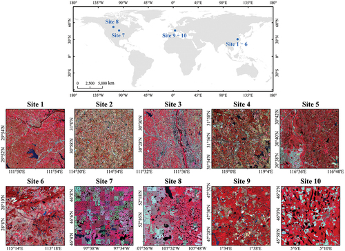
Ten study sites, each with an area of 100 km², were selected in this study (Figure 1). Sites 1–6 are located in the Yangtze River basin, China. Site 7 is located in North Dakota, USA. Site 8 is located in Saskatchewan, Canada. Sites 9–10 are located in Loir-et-Cher and Ain, France. Each site contains a large number of SWBs used for irrigation, aquaculture, and rice cultivation.

Figure 1. Locations of the ten study sites. Each study site has an area of 100 km². The false color Sentinel-2 images are composited with NIR-red-green as RGB.

2.2. Data

2.2.1. Sentinel-2 imagry

Ten Sentinel-2 multi-spectral images in the ten study sites were downloaded from the Copernicus European Space Agency hub. The Level 1C Sentinel-2 top of atmosphere (TOA) reflectance images were atmospheric corrected to surface reflectance images based on the Sen2Cor tool of SNAP software (Main-Knorn et al. 2017). In each site, a subset of Sentinel-2 images with an area of 100 km² was adopted for surface water fraction mapping (Figure 1). The ten Sentinel-2 subset images are free of opaque clouds and thin cirrus clouds based on the Sentinel-2 quality assessment band and the scene classification operator in the Sen2Cor tool. Sentinel-2 images cover the spectral range between 433 and 2280 nm, with 13 spectral bands at 10–60 m resolution. Ten bands with spatial resolutions of 10 m and 20 m were used in this study, including the blue, green, red, three vegetation red-edge bands, near-infrared (NIR) band, narrow near-infrared band, and two short-wave infrared (SWIR) bands. The Sentinel-2 images were projected onto the WGS-1984 Universal Transverse Mercator (UTM) projection.

2.2.2. Google Earth image for validation

Ten high-spatial-resolution (1 m) cloud-free Google Earth images were used as the ground truth data in Figure 2 (a₁–a₁₀). The Google Earth images were acquired temporally close to the corresponding Sentinel-2 images to reduce the impact of land cover change when assessing the surface water fraction mapping outputs from Sentinel-2 (Table 1). Each Google Earth image was projected onto the UTM projection which is the same as the corresponding Sentinel-2 image. The Google Earth images were geo-registered with the Sentinel-2 images to reduce the impact of registration errors (Hoge et al. 2003). Surface water bodies on all ten sites were digitized manually through visual interpretation on the basis of the Google Earth images to produce the 1 m water – land binary maps in Figure 2 (b₁–b₁₀) (Halabisky et al. 2016; Sall et al. 2021; Perin et al. 2022). The use of finer-spatial-resolution data with advanced interpretation models including visual interpretation through expert knowledge has shown its effectiveness to quantify the surface water maps (Olofsson et al. 2014; Pekel et al. 2016; Pickens et al. 2020). Then, the 1 m binary surface water maps were spatially degraded to 10 m resolution reference surface water fraction images to validate the accuracy of surface water fraction images. The reference surface water fraction in each Sentinel-2 pixel was calculated by dividing the total number of 1 m resolution water pixels within the pixel by 100 (Nill et al. 2022; B. Wang et al. 2022).

Figure 2. The validation images of the ten sites. (a₁−a₁₀) Google Earth RGB images used for validation, (b₁−b₁₀) surface water bodies digitized manually from Google Earth images. The blue color in (b₁−b₁₀) indicates surface water bodies.

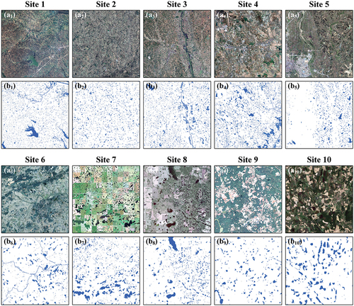
Table 1. The acquisition dates of the Sentinel-2 and Google Earth images.

Site	Date of Sentinel-2 image	Date of Google Earth image
1	21 August 2019	24 August 2019
2	26 December 2017	22 December 2017
3	27 April 2020	27 April 2020
4	2 December 2021	29 November 2021
5	7 April 2018	8 April 2018
6	10 November 2020	10 November 2020
7	20 September 2019	23 September 2019
8	12 June 2016	12 June 2016
9	6 October 2018	6 October 2018
10	14 May 2022	18 May 2022

2.3. SWBs in the ten sites

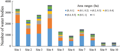
The statistics on the area of surface water bodies in each site are shown in Figure 3. The SWBs that are smaller than 1 ha are large in number at the ten sites. In particular, the number of SWBs is 3320, 2335, 2790, 3664, 1303, 938, 1515, 1109, 332, and 335 at the ten sites, respectively. The total area of SWBs smaller than 1 ha are ~377 ha (98.40% of total surface water area) at site 1, ~409 ha (98.54% of total surface water area) at site 2, ~480 ha (97.46% of total surface water area) at site 3, ~649 ha (96.92% of total surface water area) at site 4, ~268 ha (95.17% of total surface water area) at site 5, ~137 ha (86.78% of total surface water area) at site 6, ~190 ha (91.16% of total surface water area) at site 7, ~168 ha (89.45% of total surface water area) at site 8, ~69 ha (64.16% of total surface water area) at site 9, and ~39 ha (53.73% of total surface water area) at site 10. The depths of SWBs in the ten sites range from approximately 1 m to 5 m.

Figure 3. The number of water bodies in each study site.

3. Method

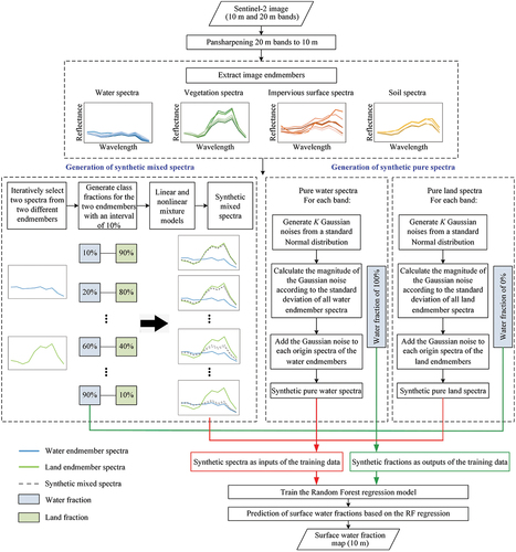
The proposed RSWFM generated 10 m spatial resolution surface water fraction maps from the Sentinel-2 images. The six 20 m Sentinel-2 bands were first downscaled to 10 m via pan-sharpening. Furthermore, according to a combination of linear and nonlinear spectral mixture models and noise-based data augmentation, synthetic spectral libraries for mixed water – land, pure water, and pure land pixels were generated based on the Sentinel-2 image endmembers and synthetic surface water fractions. With the training dataset, RF was used to construct the regression relationship between the synthetic spectra and the corresponding surface water fractions and then applied to the Sentinel-2 image to generate the surface water fraction map. A flowchart of the RSWFM is shown in Figure 4 and more details of the method are given below.

Figure 4. Flowchart of the proposed RSWFM. A mixing ratio interval of 10% is used in this study.

3.1. Sentinel-2 image pre-processing

The six Sentinel-2 20 m bands, including the three vegetation red-edge bands, narrow NIR band, and two SWIR bands, were downscaled to 10 m based on the area-to-point regression kriging (ATPRK), which uses linear regression modeling and residual downscaling to sharpen the coarse spatial resolution imagery (Q. Wang, Shi, and Atkinson 2016). ATPRK could provide sufficient spatial geometric information in downscaling the 20 m Sentinel-2 imagery in comparison with other pan-sharpening approaches (Q. Wang et al. 2016; Q. Li et al. 2022). The key of ATPRK is selecting the appropriate 10 m Sentinel-2 pan-like band used for downscaling each 20 m Sentinel-2 bands. In ATPRK, the four 10 m band were upscaled to 20 m. Then, the Pearson correlation coefficients between the 20 m band and each upscaled 10 m band were calculated, and the pan-like band used for pan-sharpening each 20 m Sentinel-2 band was determined based on the 10 m band with the highest Pearson correlation coefficients to that 20 m band (Hoge et al. 2003).

3.2. Generation of the synthetic spectral libraries

3.2.1. Endmember spectra collection

At each study site, several endmember spectra were collected directly from the Sentinel-2 image. The endmember spectra were sampled from homogeneous regions in the Sentinel-2 image based on the corresponding Google Earth image (Mitraka, Del Frate, and Carbone 2016). The size of the homogeneous region to define endmember spectra was at least 30 × 30 m. A two-level hierarchical classification scheme was used in this study (Mitraka, Del Frate, and Carbone 2016; Cooper et al. 2020; Schug et al. 2020). The first level contains four main classes including water, vegetation, impervious surface, and soil. The second level divided the first level into more detailed sub-classes so that various land cover classes can be involved in compositing the spectral library. For instance, the first level class of vegetation includes the subclasses of trees, crops, and shrubs in the second level in site 2, and the first level class of impervious includes the subclasses of building roofs and roads in the second level in site 5. The number of endmember spectra for the first level class is listed in Table 2. Because the Sentinel-2 images used for analysis were selected for different seasons, the endmember spectra for each site were used to construct the synthetic spectral library for only that particular site. Ten synthetic spectral libraries were thus constructed.

Table 2. The number of water, vegetation, impervious surface, and soil endmembers in the ten sites.

Site	Water	Vegetation	Impervious surface	Soil	Total
1	8	5	7	4	24
2	9	4	6	6	25
3	8	4	6	6	24
4	7	7	7	6	27
5	9	4	7	5	25
6	9	5	5	6	25
7	7	8	6	6	27
8	5	7	4	6	22
9	9	7	4	4	24
10	8	8	5	5	26

3.2.2. Generation of synthetic mixed spectra

RSWFM generated a series of synthetic water-vegetation-impervious surface-soil (WVIS) fractions and the corresponding synthetic mixed spectra.

First, synthetic WVIS fractions were generated. The RSWFM adopts a binary mixture model that considers a pixel composed of no more than two classes (Franke et al. 2009; Okujeni et al. 2013). Two different endmembers were first selected, and the class fractions of the two selected endmembers were assigned proportionally, as shown in Figure 4 (Okujeni et al. 2013). The mixing ratios for the two endmembers were set from 10% to 90%, with an interval of 10% to reconcile the conflicts among running time, data complexity, and redundancy. The sum of the two endmember fractions was 100%.

Synthetic mixed spectra were generated according to endmember spectra and synthetic class fractions. With each synthetic endmember fraction in the binary mixture model, two spectra, each from the corresponding endmember, were mixed to generate synthetic mixed spectra. We iteratively selected all combinations of spectra from the two endmembers in the binary mixture model to fully represent all possible spectral mixing scenarios. In each binary mixture model, both linear and nonlinear mixture models are considered for generating the synthetic mixed spectra (Okujeni et al. 2013; Okujeni, van der Linden, and Hostert 2015; Mitraka, Del Frate, and Carbone 2016). The linear and nonlinear spectral synthesis models are described in Equations (1)(1) ${\alpha }_i=\sum _{j=1}^N{a}_j(i)\cdot {\rho }_j$(1) and (2(2) ${\beta }_i={\alpha }_i+\sum _{j=1}^N\sum _{l=j}^N{b}_{j,l}(i)\cdot {\rho }_j{\rho }_l$(2) ), respectively:

(1) ${\alpha }_i=\sum _{j=1}^N{a}_j(i)\cdot {\rho }_j$(1)

(2) ${\beta }_i={\alpha }_i+\sum _{j=1}^N\sum _{l=j}^N{b}_{j,l}(i)\cdot {\rho }_j{\rho }_l$(2)

where α_i is the i^th synthetic mixed spectra using the linear spectral synthesis model, β_i is the i^th synthetic mixed spectra using the nonlinear spectral synthesis model, a_j(i) is the mixing ratio of endmember j in mixed spectra i, b_j,l(i) is a non-negativity coefficient for representing the nonlinear contribution randomly assigned from an exponential distribution with a mean value of 0.05 in mixed spectra i (Meganem et al. 2013), ρ_j and ρ_l are the spectra of endmembers j and l, respectively, and N is the number of endmembers in the mixture model.

3.2.3. Generation of synthetic pure spectra

To enhance the representability of pure endmembers in the training regression-based unmixing model, noise-based data augmentation was performed to increase the number of pure spectra and enhance the representativeness of the pure spectra. Several synthetic Gaussian noises were added to the spectra of pure water and pure land endmembers. For each endmember spectrum in Table 2, a total of K spectra vectors were generated based on Gaussian noise-based augmentation. Specifically, we assumed that ${\rho }_{b,i,k}^{water}$ is the k^th (k = 1, 2, … , K) synthetic spectrum for the i^th water endmember in the b^th spectral band, which was calculated as

(3) ${\rho }_{b,i,k}^{water}={\rho }_{b,i}^{water}+\frac{{\sigma }_b^{water}}{C}\times {\xi }_{b,i,k}^{water}$(3)

where ${\rho }_{b,i}^{water}$ is the spectrum of the b^th band in the i^th water endmember; ${\xi }_{b,i,k}^{water}$ is k^th synthetic additive Gaussian noise with zero mean and one variance in the b^th band for the i^th water endmember; and ${\sigma }_b^{water}$ is the spectrum standard deviation of the b^th band in all water endmembers, which is multiplied by the synthetic Gaussian noise. The magnitude of Gaussian noise is proportional to the standard deviation of the spectral value in the b^th band. C is a constant coefficient that controls the magnitude of the Gaussian noise.

Similarly, for land endmembers, the k^th (k = 1, 2, … , K) synthetic spectrum for the i^th land endmember in the b^th spectral band, that is, ${\rho }_{b,i,k}^{land}$, was calculated as:

(4) ${\rho }_{b,i,k}^{land}={\rho }_{b,i}^{land}+\frac{{\sigma }_b^{land}}{C}\times {\xi }_{b,i,k}^{land}$(4)

where ${\rho }_{b,i}^{land}$ is the spectrum of the b^th band in the i^th land endmember; ${\xi }_{b,i,k}^{land}$ is k^th synthetic additive Gaussian noise with zero mean and one variance in the b^th band for the i^th land endmember; and ${\sigma }_b^{land}$ is the spectrum standard deviation of the b^th band in all land endmembers, which is multiplied by the synthetic Gaussian noise.

3.3. Spectra unmixing based on RF regression

According to the aforementioned synthetic spectral library, a series of synthetic spectral values and their corresponding class fractions were generated. In the regression model, all the class fractions from vegetation, impervious surface, and soil were merged as land class fractions. The synthetic spectral values and their corresponding surface water fractions for the mixed and pure spectra were input into an RF regression to train the surface water fraction prediction model. Specifically, the synthetic spectra were input as independent variables, and the corresponding synthetic surface water fraction was input as a response variable. The number of synthetic mixed and pure spectra is dependent on the number of image endmembers, the mixing ratio interval for water and land, and the parameter K in Equations (3)(3) ${\rho }_{b,i,k}^{water}={\rho }_{b,i}^{water}+\frac{{\sigma }_b^{water}}{C}\times {\xi }_{b,i,k}^{water}$(3) and (4(4) ${\rho }_{b,i,k}^{land}={\rho }_{b,i}^{land}+\frac{{\sigma }_b^{land}}{C}\times {\xi }_{b,i,k}^{land}$(4) ). Detailed information about the number of spectra used for training the RF regression model is shown in Table 3.

Table 3. The number of spectra samples for training regression models in different sites. The number of synthetic mixed water – land spectra is mainly dependent on the mixing ratio interval, which is set as 10% in this study. The number of synthetic pure spectra is dependent on the parameter K, and this table shows the number of synthetic pure spectra with K = 500 which is adopted in model comparison in the experimental results.

Site	Number of original image endmember spectra		Number of synthetic spectra			Total
	Water	Land	Mixed water–land spectra	Pure water spectra	Pure land spectra
1	8	16	3798	4000	8000	15822
2	9	16	4104	4500	8000	16629
3	8	16	3816	4000	8000	15840
4	7	20	4914	3500	10000	18441
5	9	16	4086	4500	8000	16611
6	9	16	4122	4500	8000	16647
7	7	20	4536	3000	10000	17563
8	5	17	2916	2000	8500	13438
9	9	15	3726	4500	7500	15750
10	8	18	4482	4000	9000	17508

RF regression (Breiman 2001) is an ensemble-learning nonlinear regression algorithm based on classification and regression trees (CART). In contrast to CART, RF combines a set of individual decision trees to improve the prediction performance. To avoid overfitting with the increase in decision trees and training data, each tree was constructed using binary partitioning of random bootstrap samples at each node of this tree. The final prediction was acquired by averaging the results of all trees. Once the RF regression model was built, it was used to predict the surface water fraction map by inputting the Sentinel-2 multi-spectral image.

The RF regression model contains two main hyperparameters including the number of decision trees (ntree) and the random subset of variables at each node (mtry). The Bayesian optimizer, an iterative response surface-based global optimization algorithm, was adopted to automatically select the optimal RF hyperparameters ntree and mtry (Pelikan, Goldberg, and Cantú-Paz 1999; Wu et al. 2019). In particular, the Bayesian optimization uses Gaussian process regression to autonomously learn the next hyperparameter value set from all the information available from previous evaluations during the tuning process (Snoek, Larochelle, and Adams 2012). According to previous studies, the range of ntree was set to 1 to 600, the optimal range of mtry was set to 1 to 10 which is the total number of variables (i.e. the number of inputted Sentinel-2 bands), and the iteration of optimization was set to 50 in the Bayesian optimizer (Feng et al. 2015; DeVries et al. 2017; L. Li et al. 2018; Han et al. 2020).

4. Comparison and assessment

4.1. Comparison with different spectral unmixing methods

The proposed RSWFM was compared with two state-of-the-art unmixing algorithms: FCLS and MESMA. At each study site, the same set of endmembers (Table 2) was used with each unmixing method. In FCLS, the unmixing result is ill-posed if the number of endmembers is larger than that of spectral bands (Small 2001). To generate reliable results and reduce computational complexity, FCLS averaged the four endmembers in mapping the surface water fraction. In contrast, MESMA and RSWFM input all the endmember spectra in unmixing.

In RSWFM, the impacts of the parameters K and C in Equations (3)(3) ${\rho }_{b,i,k}^{water}={\rho }_{b,i}^{water}+\frac{{\sigma }_b^{water}}{C}\times {\xi }_{b,i,k}^{water}$(3) and (4(4) ${\rho }_{b,i,k}^{land}={\rho }_{b,i}^{land}+\frac{{\sigma }_b^{land}}{C}\times {\xi }_{b,i,k}^{land}$(4) ) were assessed. Parameter K, which determines the number of synthetic pure spectra in the training data, was set to 0, 50, 100, 200, 500, 800, 1000, and 1200. Parameter C, which controls the magnitude of Gaussian noise, was set as 0.2, 0.5, 1, 5, 10, 20, and 50. Very large values for K (K > 1200) and C (C > 50) will increase the running time and do not necessarily increase the mapping accuracy through many trials and were thus not assessed. When K = 0, RSWFM was the same as traditional regression-based unmixing without noise-based data augmentation.

4.2. Accuracy assessment

The accuracy of the predictions from the different methods was assessed by comparison with the reference surface water fraction maps produced from the Google Earth images (Figure 2 (b₁−b₁₀)). The per-pixel accuracies of the different methods were assessed using the root mean square error (RMSE) and the mean absolute error (MAE) as follows:

(5) $RMSE=\sqrt{\frac{\sum _{m=1}^M{(P_m-R_m)}^2}{M}}$(5)

(6) $MAE=\frac{\sum _{m=1}^M\left|P_m-R_m\right|}{M}$(6)

where M is the number of 10 m Sentinel-2 image pixels, P_m is the predicted surface water fraction of the m^th pixel, and R_m is the reference surface water fraction for the m^th pixel.

The percentage area error for each water body was assessed using the mean absolute percentage error (MAPE) (Chicco, Warrens, and Jurman 2021):

(7) $MAPE=\frac{\sum _{m=1}^M\left|\frac{P_m-R_m}{R_m}\right|}{M}\times 100\mathrm{\%}$(7)

where M is the number of SWBs assessed, P_m is the predicted area of m^th SWB, and R_m is the reference area of m^th SWB. An MAPE value of 0 indicates that there is no error between the predicted and reference water areas, while an MAPE value greater than 100% indicates that the predicted values are highly unreliable.

The correlation of predicted and reference SWB areas was assessed using the coefficient of determination (R²) of the fitted line in the linear regression (Wright 1921; Chicco, Warrens, and Jurman 2021):

(8) $R^2=1-\frac{\sum _{\mathrm{m}=1}^M(P_m-R_m){ }^2}{\overline{(}R-R_m){ }^2}$(8)

where M is the number of SWBs assessed, P_m is the predicted area of m^th SWB, R_m is the reference area of m^th SWB, and $\bar{R}$ is the mean reference area of all SWBs. The upper bound value of R² is 1, and the fitness performs perfectly when the R² attains 1.

5. Results

The predicted surface water fraction maps obtained from the different methods were compared. This section demonstrates the results of RSWFM without noise-based data augmentation (with K = 0, that is, no synthetic pure spectra were generated, and there is no impact from C according to Equations (3(3) ${\rho }_{b,i,k}^{water}={\rho }_{b,i}^{water}+\frac{{\sigma }_b^{water}}{C}\times {\xi }_{b,i,k}^{water}$(3) –4(4) ${\rho }_{b,i,k}^{land}={\rho }_{b,i}^{land}+\frac{{\sigma }_b^{land}}{C}\times {\xi }_{b,i,k}^{land}$(4) )) and RSWFM with noise-based data augmentation with parameters K = 100, C = 5 and K = 500, C = 5. The impacts of different K values (0, 50, 100, 200, 500, 800, 1000, and 1200) and C values (0.2, 0.5, 1, 5, 10, 20, and 50) are discussed in the discussion section.

5.1. Comparison of model performances in ten sites

The surface water fraction maps generated by FCLS, MESMA, and RSWFM at the ten sites are shown in Figure 5. FCLS unmixing overestimated the surface water fraction typically at sites 3–7 and site 9. RSWFM without noise-based data augmentation (K = 0) overestimated the surface water fraction at sites 3–9. The surface water fraction maps generated by RSWFM were more similar to the reference map than those generated by FCLS, MESMA, and RSWFM without noise-based data augmentation.

Figure 5. Comparison of surface water fraction maps using different models. (a₁−a₁₀) Reference surface water fraction maps, (b₁−b₁₀) FCLS, (c₁−c₁₀) MESMA, (d₁−d₁₀) the RSWFM with parameter K=0, (e₁−e₁₀) the RSWFM with parameter K=100 and parameter C=5, and (f₁−f₁₀) the RSWFM with parameter K=500 and parameter C=5.

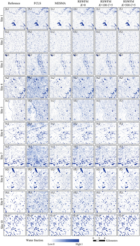
The quantitative accuracy assessment metrics of RMSEs and MAEs for the surface water fraction maps from each method are listed in Table 4. The proposed RSWFM generated the lowest RMSEs, which were lower than 0.16 for all ten sites. In general, RSWFM decreased the RMSEs by 0.01–0.11 (~30% on average) compared with FCLS and by 0.01–0.07 (~15% on average) compared with MESMA. Similarly, the RSWFM generated MAEs that were lower than 0.09 and decreased the MAEs by 0–0.11 (~46% on average) compared with FCLS. Moreover, RSWFM generated the lowest MAEs at all sites, except for sites 2, 4, and 5.

Table 4. Accuracy assessment results. The lowest values (indicating the most accurate) in each row are highlighted in bold.

Site	Metric	FCLS	MESMA	RSWFM K=0	RSWFM K=100 C=5	RSWFM K=500 C=5
1	RMSE	0.1466	0.1402	0.1408	0.1308	0.1303
	MAE	0.0747	0.0403	0.0550	0.0402	0.0355
2	RMSE	0.1125	0.1106	0.1047	0.0931	0.0894
	MAE	0.0432	0.0304	0.0576	0.0432	0.0352
3	RMSE	0.2051	0.1739	0.1487	0.1428	0.1451
	MAE	0.0920	0.0553	0.0657	0.0554	0.0518
4	RMSE	0.2438	0.1758	0.1716	0.1592	0.1589
	MAE	0.1595	0.0610	0.1114	0.0856	0.0747
5	RMSE	0.2049	0.1564	0.1504	0.1393	0.1362
	MAE	0.1125	0.0530	0.0840	0.0689	0.0604
6	RMSE	0.1801	0.1270	0.1240	0.1081	0.1094
	MAE	0.0916	0.0418	0.0587	0.0405	0.0362
7	RMSE	0.1990	0.1598	0.1267	0.1073	0.0982
	MAE	0.1418	0.0536	0.0674	0.0460	0.0363
8	RMSE	0.1500	0.1675	0.1306	0.1201	0.1182
	MAE	0.0567	0.0532	0.0572	0.0386	0.0333
9	RMSE	0.2033	0.1160	0.1310	0.1056	0.1009
	MAE	0.1223	0.0360	0.0709	0.0419	0.0335
10	RMSE	0.1385	0.1149	0.1274	0.1155	0.1126
	MAE	0.0494	0.0355	0.0611	0.0381	0.0298

RSWFMs (K = 100 and K = 500) generated lower RMSE and MAE values than the traditional regression-based unmixing without noise-based data augmentation (RSWFM with K = 0) at ten sites, showing that increasing the number of synthetic pure spectra could reduce the surface water fraction mapping error. In particular, RSWFM (K = 100 and K = 500) decreased RMSE by 0.003–0.031 (~11% on average) and decreased MAE by 0.01–0.04 (~33% on average) compared with RSWFM (K = 0).

5.2. Comparison of SWBs of different sizes, shapes, and spectral properties

The results of the surface water fractions for several SWBs of different sizes, shapes, and spectral properties from all the methods are compared in this section.

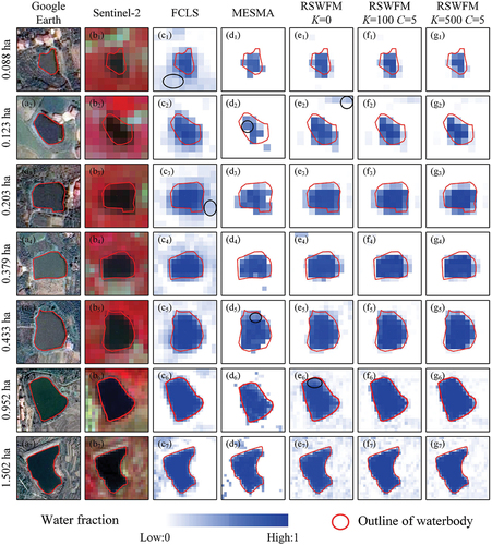
Figure 6 shows the predicted surface water fractions for SWBs of different sizes obtained from the different methods. FCLS overestimated surface water fractions for many pure land pixels, such as those highlighted by black ellipses in Figure 6 (c₁) and (c₃). MESMA underestimated the surface water fractions for many pure water pixels, such as those highlighted by black ellipses in Figure 6 (d₂) and (d₅). The traditional regression-based unmixing without noise-based data augmentation (RSWFM with K = 0) overestimated the surface water fractions for several pure land pixels, such as the black ellipse in Figure 6 (e₂), and underestimated the surface water fractions for several pure water pixels, such as the black ellipse in Figure 6 (e₆). In contrast, RSWFM with noise-based data augmentation (K = 100 and K = 500) predicted surface water fractions better in the pure land and pure water pixels generally. All the methods roughly predicted the shape of the SWBs when they were larger than approximately 0.3 ha in Figure 6. This is because large SWBs contain many pure-water pixels. All the methods failed to accurately predict the exact shape of the smallest SWB, which was 0.088 ha (first row in Figure 6). This is because a large proportion of the SWB area was located in the mixed water – land boundary pixels. This finding reveals that even though Sentinel-2 images have a relatively fine 10 m resolution, they are still challenging in mapping the SWB of small size (especially <0.1 ha, about 10 Sentinel-2 pixels).

Figure 6. Zoomed-in regions for SWB examples in different area ranges. (a₁−a₇) Google-Earth image, (b₁−b₇) Sentinel-2 image, (c₁−c₇) FCLS, (d₁−d₇) MESMA, and (e₁−e₇) the RSWFM with parameter K=0, (f₁−f₇) the RSWFM with parameters K=100 and C=5, and (g₁−g₇) the RSWFM with parameters K=500 and C=5. The Sentinel-2 near-infrared, red, and green bands are respectively mapped to RGB channels in the false color composite images in (b).

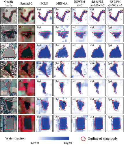
Figure 7 shows the predicted surface water fractions for SWBs of different shapes obtained using different methods. It is clear that for artificial fishponds and on-farm reservoirs that have rectangular and circular shapes, such as SWB in Figure 7 (a₇), all the methods can roughly predict the shape of these SWBs. For natural ponds with irregular shapes, none of the methods could precisely map the shape of the SWB, as shown in Figure 7 (c₄–g₄). For the linear SWB in Figure 7 (a₁), all the methods have generally mapped the shape of the SWB but failed to accurately map the regions where the river is meandering, as highlighted by black ellipses in Figure 7 (c₁–g₁). Similar results were obtained by comparing the different methods. In particular, the FCLS overestimated the surface water fraction in the vegetation regions, as shown in Figure 7 (c₂) and (c₃). MESMA underestimated the surface water fraction within the pond, as indicated by the black ellipse in Figure 7 (d₄) and (d₆). RSWFM (K = 100 and K = 500) reduced the overestimation in the vegetation regions compared with RSWFM (K = 0), as shown in Figure 7 (e₅) and (e₇), and better mapped the shape of the SWBs, showing the effectiveness of integrating noise-based data augmentation.

Figure 7. Zoomed-in regions for SWB examples with different shapes. (a₁−a₇) Google-Earth image, (b₁−b₇) Sentinel-2 image, (c₁−c₇) FCLS, (d₁−d₇) MESMA, and (e₁−e₇) the RSWFM with parameter K=0, (f₁−f₇) the proposed RSWFM with parameters K=100 and C=5, and (g₁−g₇) the proposed RSWFM with parameters K=500 and C=5. The Sentinel-2 near-infrared, red, and green bands are respectively mapped to RGB channels in the false color composite images in (b).

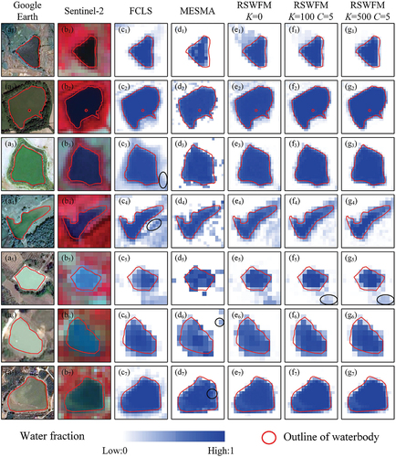
Figure 8 shows the predicted surface water fractions for SWBs with different spectral properties using different methods. The SWBs are represented as black, dark blue, light blue, and dark green in the Sentinel-2 false-color composite images in Figure 8 (b₁–b₇). In general, because FCLS averaged the spectra of different water endmembers, it overestimated the surface water fractions in the regions covered by dense vegetation, as highlighted by the black ellipse in Figure 8 (c₃). Moreover, FCLS overestimated the surface water fraction in the shadow area, as highlighted by the black ellipse in Figure 8 (c₄), because the dark shadows and water have similar spectral properties. In contrast, MESMA and RSWFM, which consider the intra-class spectral variability in water endmembers, better-distinguished water from land and reduced the overestimation of the surface water fraction in vegetation areas. MESMA overestimated the surface water in the bare region, as highlighted by the black ellipse in Figure 8 (d₆), and underestimated the surface water near the water−land boundary region, as highlighted by the black ellipse in Figure 8 (d₇). In contrast, the RSWFM maps were more similar to the real surface water of the SWBs in Figure 8 (a₁–a₇). Although RSWFM outperformed the comparators in mapping most SWBs, it predicted some flaws for some SWBs. For instance, RSWFM overestimated surface water fractions in the bare land regions highlighted in the black ellipse in Figure 8 (f₅) and (g₅), whereas MESMA better mapped the surface water fractions in this region.

Figure 8. Zoomed-in regions for SWB examples with different spectral properties. (a₁−a₇) Google-Earth image, (b₁−b₇) Sentinel-2 image, (c₁−c₇) FCLS, (d₁−d₇) MESMA, and (e₁−e₇) the proposed RSWFM with parameter K=0, (f₁−f₇) the proposed RSWFM with parameters K=100 and C=5, and (g₁−g₇) the proposed RSWFM with parameters K=500 and C=5. The Sentinel-2 near-infrared, red, and green bands are respectively mapped to RGB channels in the false color composite images in (b).

6. Discussion

6.1. Impact of RSWFM parameters

RSWFM performance depends on its parameters. In RSWFM, the parameter K controls the number of enlarged pure spectra (the number of synthetic pure spectra is K times the number of endmember spectra), and the parameter C in Equations (3(3) ${\rho }_{b,i,k}^{water}={\rho }_{b,i}^{water}+\frac{{\sigma }_b^{water}}{C}\times {\xi }_{b,i,k}^{water}$(3) –4(4) ${\rho }_{b,i,k}^{land}={\rho }_{b,i}^{land}+\frac{{\sigma }_b^{land}}{C}\times {\xi }_{b,i,k}^{land}$(4) ) controls the magnitude of the Gaussian noise added to the pure endmember spectra. Different K values (K = 0, 50, 100, 200, 500, 800, 1000, and 1200) and C values (C = 0.2, 0.5, 1, 5, 10, 20, and 50) were assessed.

The corresponding RMSE values for the surface water fraction maps are shown in Figure 9. When 0.5<C < 50, RSWFM with K > 0 generated smaller RMSE values than the traditional regression-based unmixing without noise-based data augmentation (RSWFM with K = 0) at all ten sites, showing that using noise-based data augmentation could improve the accuracy of RSWFM. In general, the lowest RMSE values were found for RSWFM with K ranging from 200 to 1000 and C ranging from 1 to 5 for all ten sites, and the difference in RMSE was less than approximately 0.015 within this range. RSWFM with a small value of K (K ≤100) generated a relatively larger RMSE than RSWFM with a relatively larger value (K ≥200), indicating that RSWFM requires a sufficient number of augmented pure endmember spectra to ensure the accuracy of the RF regression. It is also noticed that using an extremely large value of K will not necessarily decrease the RMSE (such as RSWFM with C = 5 at site 1) but will increase the complexity and running time of the RF regression model. For instance, RSWFM with K = 1000 decreased RMSE by only 0.001 but the running time doubled in comparison with RSWFM with K = 500.

Figure 9. RMSE values of surface water fraction from RSWFM using different values for the parameters CK and KC. Lighter color indicates smaller RMSE values.

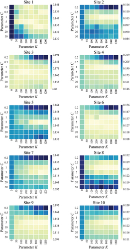
For parameter C, which controls the magnitude of the Gaussian noise in the synthetic pure endmember, neither a very large value (C = 50) nor a very small value (C = 0.2) generates a low RMSE. This is because a very large value of C indicates a small magnitude of noise, and the synthetic pure endmember spectra would not be representative of the variance in pure endmember spectra change, whereas a small value of C indicates a very large magnitude of the noise that may overestimate the variance of synthetic pure endmember spectra.

The optimal values of K and C are in the range of 200 to 1000 and 1 to 5 respectively based on the ten sites around the world. In this study, the K = 500 and C = 5 usually generated the results with the smallest RMSE. It is also suggested to select the optimal parameters for C and K on the basis of the grid search through many trials.

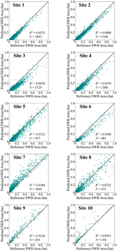
6.2. Per-SWB water area estimation

This section explores the potential of RSWFM for estimating the surface water area for each SWB. RSWFM with K = 500 and C = 5 is assessed. Water buffers were created for each SWB by expanding the water outline outward by 20 m (Halabisky et al. 2016; Sall et al. 2021). The surface water area for an SWB was calculated by summarizing the total surface water fraction of pixels in the 20 m buffer of the SWB in the RSWFM surface water fraction map. Figure 10 shows scatter plots between the reference and predicted surface water areas for SWBs smaller than 1 ha, whose buffers did not interact with other SWBs. Linear regression was used to fit the reference and predict SWB water areas, and the R² of the fitted line was used to assess the degree of match between the reference and predicted SWB water areas. RSWFM generated an R² larger than 0.85, showing a good agreement when comparing the RSWFM prediction and the reference. R² larger than 0.95 that showed the highest agreements were found in site 1, site 2, and site 6. R² smaller than 0.90 were found in site 8 (R² = 0.8722) and site 10 (R² = 0.8591) where the dense vegetation and phytoplankton have similar spectral features as the SWBs.

Figure 10. Scatter plots of the predicted SWB areas estimated by the proposed RSWFM and reference SWB areas in ten sites. The 1:1 line is shown as the black dotted line. N represents the number of SWBs used for assessment in each site. The parameters K and C used in RSWFM are 500 and 5, respectively.

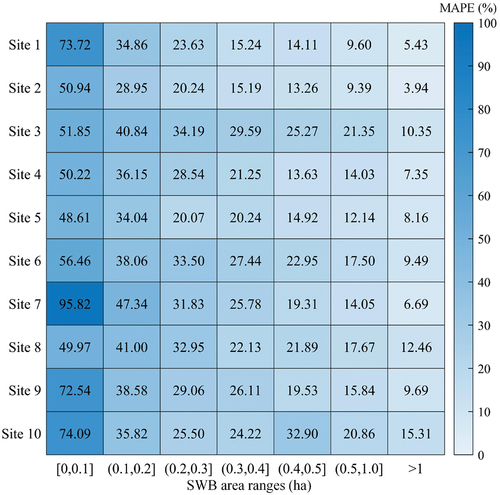
Figure 11 shows MAPEs of the predicted SWB water area for SWBs of different sizes in the ten sites; a lower MAPE indicates a better match between the predicted and the reference water area for a target SWB. Different from previous studies that mapped the SWBs smaller than 5–30 ha based on the pixel-based classification (Bie et al. 2020; Perin et al. 2021), this study explored the potential of the sub-pixel method of RSWFM in mapping SWBs smaller than 1 ha. In general, the water area estimation accuracy from the proposed RSWFM increased with the increase of area ranges except for the area range of 0.5–1 ha in site 4, the area range of 0.3–0.4 ha in site 5, and the area range of 0.4–0.5 ha in site 10. This finding is consistent with the findings of previous studies that the accuracy in mapping SWB decreases with the decrease in SWB area (Perin et al. 2022). The MAPEs for RSWFM were larger than ~ 50% when SWB was less than 0.1 ha in all ten sites, highlighting the need of mapping these very small SWBs from 10 m Sentinel-2 imagery in the future.

Figure 11. Mean absolute percentage errors (MAPEs) comparison for the estimated area of SWBs grouped into different SWB area ranges in ten sites. The selected SWBs used for MAPE estimation of each SWB area range are those with an area of corresponding SWB area range and site. The MAPEs value increase with the decrease of SWB area generally.

6.3. Limitations and future research

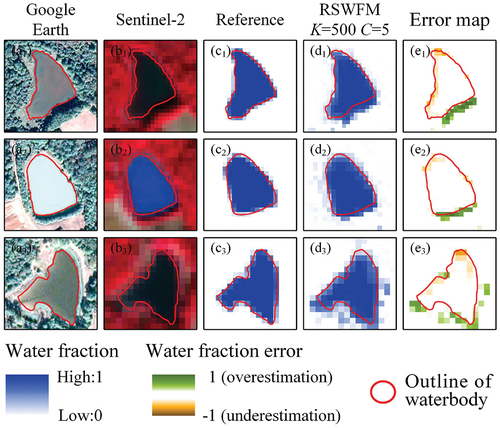
The regions where the proposed RSWFM overestimated and underestimated surface water fractions were analyzed. Since the aim of this study is to map water fractions instead of binary water maps, the metrics such as false positives or true negatives were not adopted in the analysis (Ovakoglou et al. 2021; Pantazi et al. 2022). In this study, the water fraction error images in Figure 12 were generated by subtracting the reference surface water fractions from the RSWFM predictions. In the error maps, a positive value indicates overestimation, and a negative value indicates underestimation in surface water fraction. It is found that overestimations in surface water fraction were mostly found in dense vegetation regions such as shown in Figure 12 (e₂) and (e₃) and in dark shadow regions such as shown in Figure 12 (e₁) and (e₃), because the dense vegetation and dark shadow have similar spectral features to water. The underestimations in surface water fraction were mostly found at the water – land boundaries for the SWBs.

Figure 12. Zoomed-in regions for SWB examples in the surface water fraction error map. (a₁−a₃) Google-Earth images, (b₁−b₃) Sentinel-2 images, (c₁−c₃) Reference surface water fractions, (d₁−d₃) the proposed RSWFM with parameters K=500 and C=5, and (e₁−e₃) surface water fraction error maps which were generated by subtracting the reference surface water fractions from the RSWFM predictions.

Although the proposed RSWFM decreased the RMSE compared to the classical FCLS and MESMA, limitations still exist. The proposed method is a supervised method that requires prior endmember spectra, which is the same as other supervised unmixing methods such as FCLS and MESMA. In this study, endmembers in each site were selected from each corresponding Sentinel-2 image respectively. It is noticed that different SWBs are generally variant in spectra in different regions around the world, and many SWBs are variant in spectra at different seasons. For instance, on-farm reservoirs are used to store water in the wet season and are used for irrigation for crops and become dry. It is thus necessary to collect representative endmember spectra for the study site to be analyzed and avoid selecting water endmembers from dry ponds. In this study, the image endmembers directly selected from the Sentinel-2 image with the help of very high resolution (VHR) Google Earth images were adopted. The image endmember has the advantage of reducing the impact of imaging observation condition, solar altitude, and vegetation phenology on unmixing studies (Halabisky et al. 2016; Okujeni et al. 2016; L. Li et al. 2019; Sall et al. 2021). Similar to the supervised spectral unmixing models based on the linear mixture models (Heinz 2001; Franke et al. 2009) and machine learning models (Okujeni et al. 2013, 2018), we highlighted the use of representative image endmembers when using the proposed RSWFM in unmixing the Sentinel-2 images. Another potential work is the combination of publically available online spectral libraries to construct a universal machine learning model to enhance the generalization of the proposed RSWFM. In addition, this study assessed RSWFM in ten sites with SWBs of fishponds, natural ponds, and small on-farm reservoirs in some selective regions around the world. Although this approach provided a range of SWBs a greater diversity of SWBs could be evaluated by working on a larger, even global, area. Besides, the proposed method was applied to the 10 m Sentinel-2 image in this study, and the result was that it was still challenging to accurately map SWBs that were smaller than 0.1 ha. With the development of VHR images such as PlanetScope, it would be possible to explore the potential of the RSWFM method for mapping SWBs from VHR imagery.

7. Conclusion

This study proposes a novel regression-based surface water fraction mapping method based on a synthetic spectra library for SWBs from Sentinel-2 imagery and improves the traditional spectral unmixing algorithms in mapping sub-pixel surface water fractions of SWBs. In particular, the proposed RSWFM is based on state-of-the-art regression-based unmixing using a synthetic spectral library and improves several aspects of the classical methods. RSWFM considers the water endmember in the unmixing model, whereas most regression-based unmixing masks out water pixels. RSWFM increased the number of pure endmembers by adding synthetic Gaussian noise to the spectra of pure endmembers, which is effective in dealing with the limitations of the small training dataset in the machine learning method. RSWFM considers both linear and nonlinear mixture models, which can better deal with the multiple scattering effects than the linear FCLS and MESMA models. RSWFM considers different spectral properties in water endmembers and better predicts surface water fractions than FCLS, which simply averages the water endmember spectra in the unmixing.

RSWFM was assessed at ten sites with hundreds or thousands of SWBs smaller than 1 ha. The experimental results showed that the proposed RSWFM generated high accuracy (RMSE <0.16, MAE < 0.09) in the surface water fraction map. Additionally, the proposed method generated predicted SWB areas with an R² value of the fitted linear regression greater than 0.85. Considering its good applicability for SWBs, the proposed RSWFM is particularly valuable for surface water fraction mapping of SWBs across large areas at a medium spatial resolution.

Acknowledgments

The authors would like to thank Yunning Peng, Xuliang Xiang, and Jiayuan Duan for manually interpreting the small water bodies from Google Earth images used for validation.

Disclosure statement

No potential conflict of interest was reported by the author(s).

Data availability statement

The data that support the findings of this study are available upon request from the corresponding author (Xiaodong Li, [email protected]). The codes of RSWFM and RSWFM v1.0 are available online for mapping sub-pixel surface water fractions of SWBs from Sentinel-2 images (https://github.com/PolarLan/RSWFM.git).

Additional information

Funding

This work was supported by the Natural Science Foundation of China [62071457]; the Natural Science Foundation of China [42271400]; the International Science and Technology Cooperation Project from Hubei Province, China [2022EHB018]; Science and Technology Partnership Program, Ministry of Science and Technology of China [KY201802007], Key Research Program of Frontier Sciences, Chinese Academy of Sciences [ZDBS-LY-DQC034]; Young Top-notch Talent Cultivation Program of Hubei Province, Application Foundation Frontier Project of Wuhan [2020020601012283]; and the Hubei Provincial Natural Science Foundation of China for Distinguished Young Scholars [2022CFA045].

References

- Bie, W., T. Fei, X. Liu, H. Liu, and G. Wu. 2020. “Small Water Bodies Mapped from Sentinel-2 Msi (Multispectral Imager) Imagery with Higher Accuracy.” International Journal of Remote Sensing 41 (20): 7912–25. doi:10.1080/01431161.2020.1766150.
- Breiman, L. 2001. “Random Forests.” Machine Learning 45 (1): 5–32. doi:10.1023/A:1010933404324.
- Chicco, D., M. J. Warrens, and G. Jurman. 2021. “The Coefficient of Determination R-Squared is More Informative Than Smape, Mae, Mape, MSE and RMSE in Regression Analysis Evaluation.” Peer Journal Computer Science 7: e623. doi:10.7717/peerj-cs.623.
- Cooper, S., A. Okujeni, C. Jänicke, M. Clark, S. van der Linden, and P. Hostert. 2020. “Disentangling Fractional Vegetation Cover: Regression-Based Unmixing of Simulated Spaceborne Imaging Spectroscopy Data.” Remote Sensing of Environment 246: 111856. doi:10.1016/j.rse.2020.111856.
- DeVries, B., C. Huang, M. W. Lang, J. W. Jones, W. Huang, I. F. Creed, and M. L. Carroll. 2017. “Automated Quantification of Surface Water Inundation in Wetlands Using Optical Satellite Imagery.” Remote Sensing 9 (8): 807. doi:10.3390/rs9080807.
- Downing, J. A. 2010. “Emerging Global Role of Small Lakes and Ponds: Little Things Mean a Lot.” Limnetica 29 (1): 0009–24. doi:10.23818/limn.29.02.
- Feng, Q., J. Gong, J. Liu, and Y. Li. 2015. “Flood Mapping Based on Multiple Endmember Spectral Mixture Analysis and Random Forest Classifier—The Case of Yuyao, China.” Remote Sensing 7 (9): 12539–12562. doi:10.3390/rs70912539.
- Franke, J., D. A. Roberts, K. Halligan, and G. Menz. 2009. “Hierarchical Multiple Endmember Spectral Mixture Analysis (Mesma) of Hyperspectral Imagery for Urban Environments.” Remote Sensing of Environment 113 (8): 1712–1723. doi:10.1016/j.rse.2009.03.018.
- Freitas, P., G. Vieira, J. Canário, D. Folhas, and W. F. Vincent. 2019. “Identification of a Threshold Minimum Area for Reflectance Retrieval from Thermokarst Lakes and Ponds Using Full-Pixel Data from Sentinel-2.” Remote Sensing 11 (6): 657. doi:10.3390/rs11060657.
- Gao, L., Q. Du, B. Zhang, W. Yang, and Y. Wu. 2013. “A Comparative Study on Linear Regression-Based Noise Estimation for Hyperspectral Imagery.” IEEE Journal of Selected Topics in Applied Earth Observations & Remote Sensing 6 (2): 488–498. doi:10.1109/JSTARS.2012.2227245.
- Gibbs, J. P. 1993. “Importance of Small Wetlands for the Persistence of Local Populations of Wetland-Associated Animals.” Wetlands 13 (1): 25–31. doi:10.1007/BF03160862.
- Halabisky, M., L. M. Moskal, A. Gillespie, and M. Hannam. 2016. “Reconstructing Semi-Arid Wetland Surface Water Dynamics Through Spectral Mixture Analysis of a Time Series of Landsat Satellite Images (1984–2011).” Remote Sensing of Environment 177: 171–183. doi:10.1016/j.rse.2016.02.040.
- Han, W., C. Huang, H. Duan, J. Gu, and J. Hou. 2020. “Lake Phenology of Freeze-Thaw Cycles Using Random Forest: A Case Study of Qinghai Lake.” Remote Sensing 12 (24): 4098. doi:10.3390/rs12244098.
- Heinz, D. C. 2001. “Fully Constrained Least Squares Linear Spectral Mixture Analysis Method for Material Quantification in Hyperspectral Imagery.” IEEE Transactions on Geoscience & Remote Sensing 39 (3): 529–545. doi:10.1109/36.911111.
- Hoge, W. S., D. Mitsouras, F. J. Rybicki, R. V. Mulkern, and C. -F. Westin. 2003. Registration of Multidimensional Image Data via Subpixel Resolution Phase Correlation. Paper presented at the Proceedings 2003 International Conference on Image Processing (Cat. No. 03CH37429). Barcelona, Spain. doi:10.1109/ICIP.2003.1246778.
- Holgerson, M. A., and P. A. Raymond. 2016. “Large Contribution to Inland Water Co2 and Ch4 Emissions from Very Small Ponds.” Nature Geoscience 9 (3): 222–226. doi:10.1038/ngeo2654.
- Huang, X., C. Xie, X. Fang, and L. Zhang. 2015. “Combining Pixel-And Object-Based Machine Learning for Identification of Water-Body Types from Urban High-Resolution Remote-Sensing Imagery.” IEEE Journal of Selected Topics in Applied Earth Observations & Remote Sensing 8 (5): 2097–2110. doi:10.1109/JSTARS.2015.2420713.
- Jamali, A., M. Mahdianpari, B. Brisco, J. Granger, F. Mohammadimanesh, and B. Salehi. 2021. “Deep Forest Classifier for Wetland Mapping Using the Combination of Sentinel-1 and Sentinel-2 Data.” GIScience & Remote Sensing 58 (7): 1072–1089. doi:10.1080/15481603.2021.1965399.
- Jarchow, C. J., B. H. Sigafus, E. Muths, and B. R. Hossack. 2020. “Using Full and Partial Unmixing Algorithms to Estimate the Inundation Extent of Small, Isolated Stock Ponds in an Arid Landscape.” Wetlands 40 (3): 563–575. doi:10.1007/s13157-019-01201-7.
- Kim, S. M., S. H. Yoon, S. Ju, and J. Heo. 2018. “Monitoring and Analyzing Water Area Variation of Lake Enriquillo, Dominican Republic by Integrating Multiple Endmember Spectral Mixture Analysis and Modis Data.” Ecology and Resilient Infrastructure 5 (2): 59–71. doi:10.17820/eri.2018.5.2.059.
- Lehner, B., and P. Döll. 2004. “Development and Validation of a Global Database of Lakes, Reservoirs and Wetlands.” Journal of Hydrology 296 (1–4): 1–22. doi:10.1016/j.jhydrol.2004.03.028.
- Liang, J., and D. Liu. 2021. “Automated Estimation of Daily Surface Water Fraction from Modis and Landsat Images Using Gaussian Process Regression.” International Journal of Remote Sensing 42 (11): 4261–4283. doi:10.1080/01431161.2021.1892859.
- Li, Q., B. Barrett, R. Williams, T. Hoey, and R. Boothroyd. 2022. “Enhancing Performance of Multi-Temporal Tropical River Landform Classification Through Downscaling Approaches.” International Journal of Remote Sensing 43 (17): 6445–6462. doi:10.1080/01431161.2022.2139164.
- Li, X., F. Ling, G. M. Foody, D. S. Boyd, L. Jiang, Y. Zhang, P. Zhou, Y. Wang, R. Chen, and Y. Du. 2021. “Monitoring High Spatiotemporal Water Dynamics by Fusing Modis, Landsat, Water Occurrence Data and Dem.” Remote Sensing of Environment 265: 112680. doi:10.1016/j.rse.2021.112680.
- Ling, F., D. Boyd, Y. Ge, G. M. Foody, X. Li, L. Wang, Y. Zhang, L. Shi, C. Shang, and X. Li. 2019. “Measuring River Wetted Width from Remotely Sensed Imagery at the Subpixel Scale with a Deep Convolutional Neural Network.” Water Resources Research 55 (7): 5631–5649. doi:10.1029/2018WR024136.
- Ling, F., X. Li, G. M. Foody, D. Boyd, Y. Ge, X. Li, and Y. Du. 2020. “Monitoring Surface Water Area Variations of Reservoirs Using Daily Modis Images by Exploring Sub-Pixel Information.” Isprs Journal of Photogrammetry & Remote Sensing 168: 141–152. doi:10.1016/j.isprsjprs.2020.08.008.
- Li, L., A. Skidmore, A. Vrieling, and T. Wang. 2019. “A New Dense 18-Year Time Series of Surface Water Fraction Estimates from Modis for the Mediterranean Region.” Hydrology and Earth System Sciences 23 (7): 3037–3056. doi:10.5194/hess-23-3037-2019.
- Liu, H., B. He, Y. Zhou, X. Yang, X. Zhang, F. Xiao, Q. Feng, S. Liang, X. Zhou, and C. Fu. 2021. “Eutrophication Monitoring of Lakes in Wuhan Based on Sentinel-2 Data.” GIScience & Remote Sensing 58 (5): 776–798. doi:10.1080/15481603.2021.1940738.
- Liu, C., J. Shi, X. Liu, Z. Shi, and J. Zhu. 2020. “Subpixel Mapping of Surface Water in the Tibetan Plateau with Modis Data.” Remote Sensing 12 (7): 1154. doi:10.3390/rs12071154.
- Li, L., A. Vrieling, A. Skidmore, T. Wang, and E. Turak. 2018. “Monitoring the Dynamics of Surface Water Fraction from Modis Time Series in a Mediterranean Environment.” International Journal of Applied Earth Observation and Geoinformation 66: 135–145. doi:10.1016/j.jag.2017.11.007.
- Ludwig, C., A. Walli, C. Schleicher, J. Weichselbaum, and M. Riffler. 2019. “A Highly Automated Algorithm for Wetland Detection Using Multi-Temporal Optical Satellite Data.” Remote Sensing of Environment 224: 333–351. doi:10.1016/j.rse.2019.01.017.
- Lv, M., S. Wu, M. Ma, P. Huang, Z. Wen, and J. Chen. 2022. “Small Water Bodies in China: Spatial Distribution and Influencing Factors.” Science China Earth Sciences 65 (8): 1431–1448. doi:10.1007/s11430-021-9939-5.
- Mahdianpari, M., H. Jafarzadeh, J. E. Granger, F. Mohammadimanesh, B. Brisco, B. Salehi, S. Homayouni, and Q. Weng. 2020. “A Large-Scale Change Monitoring of Wetlands Using Time Series Landsat Imagery on Google Earth Engine: A Case Study in Newfoundland.” GIScience & Remote Sensing 57 (8): 1102–1124. doi:10.1080/15481603.2020.1846948.
- Main-Knorn, M., B. Pflug, J. Louis, V. Debaecker, U. Müller-Wilm, and F. Gascon. 2017. Sen2cor for Sentinel-2. Paper presented at the Image and Signal Processing for Remote Sensing XXIII. Warsaw, Poland. doi:10.1117/12.2278218.
- Matsushita, B., W. Yang, P. Chang, F. Yang, and T. Fukushima. 2012. “A Simple Method for Distinguishing Global Case-1 and Case-2 Waters Using Seawifs Measurements.” Isprs Journal of Photogrammetry & Remote Sensing 69: 74–87. doi:10.1016/j.isprsjprs.2012.02.008.
- Meganem, I., P. Déliot, X. Briottet, Y. Deville, and S. Hosseini. 2013. “Linear–Quadratic Mixing Model for Reflectances in Urban Environments.” IEEE Transactions on Geoscience & Remote Sensing 52 (1): 544–558. doi:10.1109/TGRS.2013.2242475.
- Mitraka, Z., F. Del Frate, and F. Carbone. 2016. “Nonlinear Spectral Unmixing of Landsat Imagery for Urban Surface Cover Mapping.” IEEE Journal of Selected Topics in Applied Earth Observations & Remote Sensing 9 (7): 3340–3350. doi:10.1109/JSTARS.2016.2522181.
- Nill, L., I. Grünberg, T. Ullmann, M. Gessner, J. Boike, and P. Hostert. 2022. “Arctic Shrub Expansion Revealed by Landsat-Derived Multitemporal Vegetation Cover Fractions in the Western Canadian Arctic.” Remote Sensing of Environment 281: 113228. doi:10.1016/j.rse.2022.113228.
- Okujeni, A., F. Canters, S. D. Cooper, J. Degerickx, U. Heiden, P. Hostert, F. Priem, D. A. Roberts, B. Somers, and S. van der Linden. 2018. “Generalizing Machine Learning Regression Models Using Multi-Site Spectral Libraries for Mapping Vegetation-Impervious-Soil Fractions Across Multiple Cities.” Remote Sensing of Environment 216: 482–496. doi:10.1016/j.rse.2018.07.011.
- Okujeni, A., S. van der Linden, and P. Hostert. 2015. “Extending the Vegetation–Impervious–Soil Model Using Simulated Enmap Data and Machine Learning.” Remote Sensing of Environment 158: 69–80. doi:10.1016/j.rse.2014.11.009.
- Okujeni, A., S. van der Linden, S. Suess, and P. Hostert. 2016. “Ensemble Learning from Synthetically Mixed Training Data for Quantifying Urban Land Cover with Support Vector Regression.” IEEE Journal of Selected Topics in Applied Earth Observations & Remote Sensing 10 (4): 1640–1650. doi:10.1109/JSTARS.2016.2634859.
- Okujeni, A., S. van der Linden, L. Tits, B. Somers, and P. Hostert. 2013. “Support Vector Regression and Synthetically Mixed Training Data for Quantifying Urban Land Cover.” Remote Sensing of Environment 137: 184–197. doi:10.1016/j.rse.2013.06.007.
- Olofsson, P., G. M. Foody, M. Herold, S. V. Stehman, C. E. Woodcock, and M. A. Wulder. 2014. “Good Practices for Estimating Area and Assessing Accuracy of Land Change.” Remote Sensing of Environment 148: 42–57. doi:10.1016/j.rse.2014.02.015.
- Otsu, N. 1979. “A Threshold Selection Method from Gray-Level Histograms.” IEEE Transactions on Systems, Man, and Cybernetics 9 (1): 62–66. doi:10.1109/TSMC.1979.4310076.
- Ovakoglou, G., I. Cherif, T. K. Alexandridis, X. -E. Pantazi, A. -A. Tamouridou, D. Moshou, X. Tseni, I. Raptis, S. Kalaitzopoulou, and S. Mourelatos. 2021. “Automatic Detection of Surface-Water Bodies from Sentinel-1 Images for Effective Mosquito Larvae Control.” Journal of Applied Remote Sensing 15 (1): 014507. doi:10.1117/1.JRS.15.014507.
- Pantazi, X. E., A. A. Tamouridou, D. Moshou, I. Cherif, G. Ovakoglou, X. Tseni, S. Kalaitzopoulou, S. Mourelatos, and T. K. Alexandridis. 2022. “Evaluation of Machine Learning Approaches for Surface Water Monitoring Using Sentinel-1 Data.” Journal of Applied Remote Sensing 16 (4): 044501. doi:10.1117/1.JRS.16.044501.
- Pekel, J. F., A. Cottam, N. Gorelick, and A. S. Belward. 2016. “High-Resolution Mapping of Global Surface Water and Its Long-Term Changes.” Nature 540 (7633): 418–422. doi:10.1038/nature20584.
- Pelikan, M., D. E. Goldberg, and E. Cantú-Paz. 1999. Boa: The Bayesian Optimization Algorithm. In Proceedings of the 1st Annual Conference on Genetic and Evolutionary Computation, 1: 525–532. Morgan Kaufmann Publishers Inc.
- Perin, V., S. Roy, J. Kington, T. Harris, M. G. Tulbure, N. Stone, T. Barsballe, M. Reba, and M. A. Yaeger. 2021. “Monitoring Small Water Bodies Using High Spatial and Temporal Resolution Analysis Ready Datasets.” Remote Sensing 13 (24): 5176. doi:10.3390/rs13245176.
- Perin, V., M. G. Tulbure, M. D. Gaines, M. L. Reba, and M. A. Yaeger. 2022. “A Multi-Sensor Satellite Imagery Approach to Monitor On-Farm Reservoirs.” Remote Sensing of Environment 270: 112796. doi:10.1016/j.rse.2021.112796.
- Peterson, K. T., V. Sagan, and J. J. Sloan. 2020. “Deep Learning-Based Water Quality Estimation and Anomaly Detection Using Landsat-8/sentinel-2 Virtual Constellation and Cloud Computing.” GIScience & Remote Sensing 57 (4): 510–525. doi:10.1080/15481603.2020.1738061.
- Pickens, A. H., M. C. Hansen, M. Hancher, S. V. Stehman, A. Tyukavina, P. Potapov, B. Marroquin, and Z. Sherani. 2020. “Mapping and Sampling to Characterize Global Inland Water Dynamics from 1999 to 2018 with Full Landsat Time-Series.” Remote Sensing of Environment 243: 111792. doi:10.1016/j.rse.2020.111792.
- Pi, X., Q. Luo, L. Feng, Y. Xu, J. Tang, X. Liang, E. Ma, R. Cheng, R. Fensholt, and M. Brandt. 2022. “Mapping Global Lake Dynamics Reveals the Emerging Roles of Small Lakes.” Nature Communications 13 (1): 1–12. doi:10.1038/s41467-022-33239-3.
- Polishchuk, Y., A. Bogdanov, I. Muratov, V. Polishchuk, A. Lim, R. Manasypov, L. Shirokova, and O. Pokrovsky. 2018. “Minor Contribution of Small Thaw Ponds to the Pools of Carbon and Methane in the Inland Waters of the Permafrost-Affected Part of the Western Siberian Lowland.” Environmental Research Letters 13 (4): 045002. doi:10.1088/1748-9326/aab046.
- Powell, R. L., D. A. Roberts, P. E. Dennison, and L. L. Hess. 2007. “Sub-Pixel Mapping of Urban Land Cover Using Multiple Endmember Spectral Mixture Analysis: Manaus, Brazil.” Remote Sensing of Environment 106 (2): 253–267. doi:10.1016/j.rse.2006.09.005.
- Priem, F., A. Okujeni, S. van der Linden, and F. Canters. 2019. “Comparing Map-Based and Library-Based Training Approaches for Urban Land-Cover Fraction Mapping from Sentinel-2 Imagery.” International Journal of Applied Earth Observation and Geoinformation 78: 295–305. doi:10.1016/j.jag.2019.02.003.
- Raymond, P. A., J. Hartmann, R. Lauerwald, S. Sobek, C. McDonald, M. Hoover, D. Butman, R. Striegl, E. Mayorga, and C. Humborg. 2013. “Global Carbon Dioxide Emissions from Inland Waters.” Nature 503 (7476): 355–359. doi:10.1038/nature12760.
- Ray, T. W., and B. C. Murray. 1996. “Nonlinear Spectral Mixing in Desert Vegetation.” Remote Sensing of Environment 55 (1): 59–64. doi:10.1016/0034-4257(95)00171-9.
- Rover, J., B. K. Wylie, and L. Ji. 2010. “A Self-Trained Classification Technique for Producing 30 M Percent-Water Maps from Landsat Data.” International Journal of Remote Sensing 31 (8): 2197–2203. doi:10.1080/01431161003667455.
- Sall, I., C. J. Jarchow, B. H. Sigafus, L. A. Eby, M. J. Forzley, and B. R. Hossack. 2021. “Estimating Inundation of Small Waterbodies with Sub‐Pixel Analysis of Landsat Imagery: Long‐Term Trends in Surface Water Area and Evaluation of Common Drought Indices.” Remote Sensing in Ecology and Conservation 7 (1): 109–124. doi:10.1002/rse2.172.
- Schug, F., D. Frantz, A. Okujeni, S. van Der Linden, and P. Hostert. 2020. “Mapping Urban-Rural Gradients of Settlements and Vegetation at National Scale Using Sentinel-2 Spectral-Temporal Metrics and Regression-Based Unmixing with Synthetic Training Data.” Remote Sensing of Environment 246: 111810. doi:10.1016/j.rse.2020.111810.
- Schug, F., A. Okujeni, J. Hauer, P. Hostert, J. Ø. Nielsen, and S. van der Linden. 2018. “Mapping Patterns of Urban Development in Ouagadougou, Burkina Faso, Using Machine Learning Regression Modeling with Bi-Seasonal Landsat Time Series.” Remote Sensing of Environment 210: 217–228. doi:10.1016/j.rse.2018.03.022.
- Senf, C., J. Laštovička, A. Okujeni, M. Heurich, and S. van der Linden. 2020. “A Generalized Regression-Based Unmixing Model for Mapping Forest Cover Fractions Throughout Three Decades of Landsat Data.” Remote Sensing of Environment 240: 111691. doi:10.1016/j.rse.2020.111691.
- Small, C. 2001. “Estimation of Urban Vegetation Abundance by Spectral Mixture Analysis.” International Journal of Remote Sensing 22 (7): 1305–1334. doi:10.1080/01431160151144369.
- Snoek, J., H. Larochelle, and R. P. Adams. 2012. “Practical Bayesian Optimization of Machine Learning Algorithms.“ Present at Advances in Neural Information Processing Systems 25. Lake Tahoe, Nevada, United States.
- Suess, S., S. van der Linden, and A. Okujeni, P. P. Griffiths, J. Leitão, M. Schwieder, and P. Hostert. 2018. “Characterizing 32 Years of Shrub Cover Dynamics in Southern Portugal Using Annual Landsat Composites and Machine Learning Regression Modeling.” Remote Sensing of Environment 219: 353–364. doi:10.1016/j.rse.2018.10.004.
- Vanthof, V., and R. Kelly. 2019. “Water Storage Estimation in Ungauged Small Reservoirs with the Tandem-X Dem and Multi-Source Satellite Observations.” Remote Sensing of Environment 235: 111437. doi:10.1016/j.rse.2019.111437.
- Vörösmarty, C. J., P. B. McIntyre, M. O. Gessner, D. Dudgeon, A. Prusevich, P. Green, S. Glidden, S. E. Bunn, C. A. Sullivan, and C. R. Liermann. 2010. “Global Threats to Human Water Security and River Biodiversity.” Nature 467 (7315): 555–561. doi:10.1038/nature09440.
- Wang, B., Z. Chen, L. Wu, X. Yang, and Y. Zhou. 2022. “Sada-Net: A Shape Feature Optimization and Multiscale Context Information-Based Water Body Extraction Method for High-Resolution Remote Sensing Images.” IEEE Journal of Selected Topics in Applied Earth Observations & Remote Sensing 15: 1744–1759. doi:10.1109/JSTARS.2022.3146275.
- Wang, Y., X. Li, P. Zhou, L. Jiang, and Y. Du. 2022. “Ahswfm: Automated and Hierarchical Surface Water Fraction Mapping for Small Water Bodies Using Sentinel-2 Images.” Remote Sensing 14 (7): 1615. doi:10.3390/rs14071615.
- Wang, S., M. Shen, W. Liu, Y. Ma, H. Shi, J. Zhang, and D. Liu. 2022. “Developing Remote Sensing Methods for Monitoring Water Quality of Alpine Rivers on the Tibetan Plateau.” GIScience & Remote Sensing 59 (1): 1384–1405. doi:10.1080/15481603.2022.2116078.
- Wang, Q., W. Shi, and P. M. Atkinson. 2016. “Area-To-Point Regression Kriging for Pan-Sharpening.” Isprs Journal of Photogrammetry & Remote Sensing 114: 151–165. doi:10.1016/j.isprsjprs.2016.02.006.
- Wang, Q., W. Shi, Z. Li, and P. M. Atkinson. 2016. “Fusion of Sentinel-2 Images.” Remote Sensing of Environment 187: 241–252. doi:10.1016/j.rse.2016.10.030.
- Wang, X., X. Xiao, Z. Zou, J. Dong, Y. Qin, R. B. Doughty, M. A. Menarguez, B. Chen, J. Wang, and H. Ye. 2020. “Gainers and Losers of Surface and Terrestrial Water Resources in China During 1989–2016.” Nature Communications 11 (1): 1–12. doi:10.1038/s41467-020-17103-w.
- Wang, X., S. Xie, X. Zhang, C. Chen, H. Guo, J. Du, and Z. Duan. 2018. “A Robust Multi-Band Water Index (Mbwi) for Automated Extraction of Surface Water from Landsat 8 Oli Imagery.” International Journal of Applied Earth Observation and Geoinformation 68: 73–91. doi:10.1016/j.jag.2018.01.018.
- Worden, J., K. M. de Beurs, J. Koch, and B. C. Owsley. 2021. “Application of Spectral Index-Based Logistic Regression to Detect Inland Water in the South Caucasus.” Remote Sensing 13 (24): 5099. doi:10.3390/rs13245099.
- Wright, S. 1921. “Correlation and Causation.“ Journal of agricultural research 20 (7): 557–585. https://handle.nal.usda.gov/10113/IND43966364.
- Wu, J., X. Chen, H. Zhang, L. Xiong, H. Lei, and S. Deng. 2019. “Hyperparameter Optimization for Machine Learning Models Based on Bayesian Optimization.” Journal of Electronic Science and Technology 17 (1): 26–40. doi:10.11989/JEST.1674-862X.80904120.
- Yang, X., Q. Chu, L. Wang, and M. Yu. 2022. “Water Body Super-Resolution Mapping Based on Multiple Endmember Spectral Mixture Analysis and Multiscale Spatio-Temporal Dependence.” Remote Sensing 14 (9): 2050. doi:10.3390/rs14092050.
- Zhang, C., Y. Chen, and D. Lu. 2015. “Mapping the Land-Cover Distribution in Arid and Semiarid Urban Landscapes with Landsat Thematic Mapper Imagery.” International Journal of Remote Sensing 36 (17): 4483–4500. doi:10.1080/01431161.2015.1084552.