Monitoring and understanding chlorophyll-a concentration changes in lakes in northeastern China using MERIS and OLCI satellite data

ABSTRACT

Lakes in the Northeast Plains-Mountain Lake Region (NPLR) of China face severe risks of eutrophication due to climate change and intensive anthropogenic pressures. As a vital indicator for eutrophication status, the dynamics of chlorophyll-a (Chl-a) concentrations in NPLR lakes were, for the first time, comprehensively investigated in this study. A support vector regression (SVR)-based model was established and applied to the MERIS (2003–2011) and OLCI (2016–2019) observations to derive a long-term Chl-a record for 33 NPLR lakes. The NPLR lakes exhibited a climatological annual mean Chl-a of 12.3 mg m⁻³, ranging from 6.8 to 18.6 mg m⁻³ among the 33 studied lakes. During the study period, 11 lakes exhibited statistically significant increases in Chl-a concentrations (p < 0.05), and 3 lakes showed significantly decreasing trends. Spatially, lakes in lowland regions had higher Chl-a than those in mountainous regions. This study quantified the relative importance of seven explanatory factors in influencing interannual Chl-a changes for each lake. Results showed statistically significant impacts of agricultural fertilizer (10 lakes), wastewater (4 lakes), runoff (7 lakes), and wind (5 lakes) in affecting the interannual variations of Chl-a. The decreases in Chl-a were primarily attributed to the reduced livestock excrement. Compared to hydro-climatic factors, anthropogenic pressures (i.e. agriculture fertilizer, livestock excrement, and wastewater discharge) had more significant impacts on the interannual variations of Chl-a, accounting for more than 50% of 18 lakes. This study enhances our understanding of the long-term Chl-a dynamics in NPLR lakes and their responses to hydro-climatic factors and anthropogenic forcing. These findings are valuable for basin-scale water environment protection and sustainable development.

KEYWORDS:

• Chlorophyll-a
• reservoirs and lakes
• human activity
• MERIS
• OLCI
• northeastern China

1. Introduction

Inland water plays a vital role in providing essential water resources for human living, economic and social development, and biodiversity maintenance (Pahlevan et al. 2019). However, due to climate change and intensive human activities, inland lakes (including natural lakes and man-constructed reservoirs) worldwide are exposed to unprecedented eutrophication pressure, which seriously threatens eco-environmental security (Chen, Huang, and Tang 2020; Ho, Michalak, and Pahlevan 2019). As such, a comprehensive understanding of changes in the water environment in response to hydro-climatic factors and human activities can provide scientific support for maintaining the balance between regional water environment protection and socio-economic development.

As field measurements and laboratory analyses require high human resources and financial investments, water quality records with continuous tempo-spatial coverage have been a long-standing constraint on water environmental research. Fortunately, rapidly developing remote sensing technology has brought new perspectives to water environment monitoring (Matthews, Bernard, and Winter 2010). As an important indicator of water eutrophication status, chlorophyll-a (Chl-a) concentration is highly related to the biogeochemical cycling processes in lakes and has been widely applied in water environment monitoring and evaluations (Attila et al. 2018; Huovinen et al. 2019). Previous studies on Chl-a monitoring in Chinese lakes were mainly focused on the East Plain Region and Yungui Plateau Region (Chen, Huang, and Tang 2020; Han et al. 2014). However, to date, no systematic efforts have been devoted to comprehensively revealing the Chl-a variations of large lakes in northeastern China. This area holds ecological significance due to its abundant distribution of lakes. Meanwhile, the extensive agricultural, industrial, and residential activities in these regions have resulted in high nutrient loading into these lakes (Wang et al. 2013), thereby posing substantial threats to their aquatic ecosystem health.

Chl-a monitoring for inland turbid waters, such as lakes in northeastern China, has been commonly recognized as a challenging problem in water color remote sensing because the strong signals induced by sediment particles made it difficult to identify accurate Chl-a information from the remotely detected radiance (Gitelson et al. 2008). Though there have been various empirical or semi-analytical Chl-a models proposed for turbid waters (Gower et al. 2005; Mishra, Schaeffer, and Keith 2014; Moses et al. 2009), considering that the optical environment of inland waters may vary significantly, the generalizability of these models appeared to be inadequate in different regions (Jiang et al. 2020). The emerging artificial intelligence algorithms have provided new opportunities for mining the complex relationships between Chl-a and water-leaving radiance for inland waters and have gained several successful attempts worldwide. For instance, Guan et al. (2020) achieved long-term Chl-a monitoring of 51 lakes on the Yangtze Plain using a support vector regression (SVR)-based piecewise model, with the mean relative error of Chl-a predictions of less than 25%. Li et al. (2021) indicated the promising performance of machine learning methods in predicting Chl-a concentrations compared to the conventional band or band ratio algorithms spanning 45 large lakes in China. Aptoula and Ariman (2021) and García-Nieto et al. (2020) applied the convolutional neural network (CNN) and Gaussian process regression (GPR) in Chl-a monitoring in Lake Balik (Turkey) and Tanes Reservoir (Northern Spain), respectively.

Among the various ocean color measurements, the Medium Resolution Imaging Spectrometer (MERIS, 2002–2011) and Ocean and Land Color Instrument (OLCI, 2016-present) had incomparable advantages in remote estimations of Chl-a, owing to their satisfactory spectral resolution (15 bands for MERIS and 21 bands for OLCI with a bandwidth of ~10 nm), high temporal frequency (1–3 days), and modest spatial resolution (300 m) (Smith, Robertson Lain, and Bernard 2018). With the observations of these two instruments, this study aims to provide the basis for understanding the temporal and spatial Chl-a dynamics and influencing factors of lakes in northeastern China. The specific objectives are 1) to establish a locally practical model for retrieving Chl-a concentration of lakes in northeastern China, 2) to delineate the long-term spatial and temporal variability of Chl-a with MERIS and OLCI observations, and 3) to explore the main driving forces, including hydro-climatic factors (i.e. air temperature, wind speed, precipitation, and runoff) and anthropogenic pressures (i.e. agriculture fertilizer, livestock excrement, and wastewater discharge), to the long-term phytoplankton biomass variations in these lakes. This study will contribute to a better knowledge of the ecological responses of lakes to hydro-climatic factors and anthropogenic pressures in northeastern China and provide crucial information for regional/national ecological restoration and water resources management.

2. Study area and datasets

2.1. Study area

The Northeast Plain-Mountain Lake Region (NPLR, 122°E-133°E, 42°N-47°N) is home to more than 400 lakes larger than 1 km², accounting for approximately one-fifth of lakes in China. These lakes are mainly distributed along the three major rivers, namely the Nen River, the Second Songhua River, and the Songhua River, and in the mountainous regions. Lakes are hydrologically connected to the major rivers or tributaries through natural rivers or manufactured channels. 33 lakes with a surface area greater than 15 km² are selected for the Chl-a examination in this study, as shown in Figure 1. The basic information for each lake is listed in Table 1. The overall water quality conditions of these lakes belong to II-V categories referring to the Environmental Quality Standard for Surface Water (GB3838–2002) (MEP 2002). The total nitrogen and total phosphorus concentrations of lakes during field measurements are given in Table S1 in the supplementary materials.

Figure 1. Spatial distributions of the 33 examined lakes (>15 km²) in NPLR. The land-use type distribution is mapped according to the National land cover dataset (NLCD) record with 1km resolutions in 2015. Note that Lake Xingkai is a transboundary water body shared by China and Russia. An asterisk (*) beside lake names denotes lakes in mountainous areas.

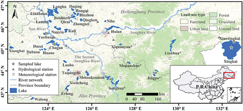
Table 1. Basic information of the examined lakes and Pearson correlation coefficients (r) between the annual mean Chl-a and annual mean values of the seven explanatory variables during the study period. “*” denotes a statistically significant correlation at the p < 0.05 level, and “NA” denotes data unavailable.

	Lon	Lat	Area	Mean depth	Chl-a	Air temperature	Wind	Precipitation	Runoff	Fertilizer	Excrement	Wastewater
Lake	(°)	(°)	(km^2)	(m)	(mg/m^3)	(℃)	(m/s)	(mm)	(m^3/s)	(10^4t)	(10^4t)	(10^4t)
Chagan	124.3	45.3	300	3.5	17.1	0.32	0.60*	−0.27	0.61*	−0.51	0.55*	−0.16
Yueliang	123.8	45.7	206	2.3	12.4	−0.09	−0.07	0.43	0.74*	0.15	0.17	0.28
Lianhuan	124.2	46.7	318	2.2	12.8	0.13	−0.08	−0.21	−0.39	−0.61*	0.62*	0.66*
Longhu	124.4	46.7	131	2.7	12.7	0.05	−0.27	0.48	0.40	−0.11	0.29	0.20
Xianghai^R	122.3	45	71	4.5	13.4	0.08	−0.42	0.39	−0.55*	0.14	0.17	0.05
Huaao	123.8	45	36	1.7	14.8	0.05	−0.49	0.23	−0.11	0.65*	0.35	0.78*
Daozi	123.6	45	19	3.2	13.7	−0.23	0.19	−0.27	0.37	0.30	0.37	0.04
Dabusu	123.6	45	35.2	1.2	16.4	0.03	0.29	−0.66*	0.03	0.25	0.02	−0.02
Boluo	124.8	44.4	62	1.3	14.3	0.22	−0.09	−0.28	NA	0.09	0.45	0.75*
Taipingchi^R	124.9	44.1	25	2.5	18.2	0.06	−0.24	0.15	NA	−0.04	0.10	0.40
Xinlicheng^R	125.4	44.6	51	6	9.5	0.16	0.43	−0.27	−0.61*	0.05	0.64*	−0.16
Shitoukoumen^R	125.8	43.9	84	3.3	12.6	0.14	−0.21	−0.46	−0.60*	0.60*	0.46	0.05
Daqing^R	125.1	46.8	82	3	9.9	0.34	0.66*	0.11	−0.09	0.19	0.39	0.53
Nanyin^R	124.5	45.9	54	3.5	11.7	0.40	−0.51	0.26	0.27	0.62*	0.49	0.17
Kuli	124.8	45.6	90	2.5	18.6	0.32	−0.71*	0.05	−0.63*	0.71*	0.40	−0.06
Qingken	125.5	46.4	53	1.2	12.3	0.20	0.09	0.46	−0.35	0.89*	−0.37	0.58*
Hongqi^R	125.2	46.6	35	2.8	8.8	0.17	0.68*	0.28	0.34	0.35	−0.26	0.63*
Beishierli	125.2	46.5	74	1.7	15.2	0.11	−0.11	0.23	−0.38	0.24	−0.44	−0.22
Zhongnei	125	46.3	33	1.6	16.0	−0.30	−0.24	0.56*	−0.22	0.71*	0.21	−0.23
Qicai	125.1	46.3	16	1.5	16.4	−0.23	−0.46	0.23	−0.31	0.63*	0.57*	−0.39
Binzhou	125.3	46.6	46	1.8	13.7	0.43	−0.53	−0.20	−0.11	0.22	0.82*	0.70*
Lamasi	124.1	46.3	60	3	17.2	0.36	−0.12	−0.23	0.54*	−0.35	−0.04	0.09
Wolong	122.8	42.7	60	1.2	12.9	0.67*	−0.46	−0.11	NA	0.36	−0.39	−0.50
Nihe^R	126.6	46.3	44	2.6	13.2	0.09	−0.49	−0.19	NA	0.40	0.35	−0.14
Hulan	127	46.4	192	2.5	11.5	0.14	−0.60*	−0.58*	0.19	−0.50	0.58*	0.69*
Xiquanyan^R	127.3	45.3	41	12	7.5	0.57*	−0.47	0.44	−0.26	0.77*	0.68*	−0.41
Mopanshan^R	127.8	44.5	28	23	6.8	0.56*	0.34	0.41	0.61*	0.60*	−0.31	−0.49
Erlong^R	124.8	43.2	170	10	9.4	0.05	0.72*	0.18	NA	0.56*	−0.29	0.71*
Songhua^R	126.9	43.6	425	30	7.2	0.08	0.33	0.48	0.55*	0.59*	0.60*	0.52
Jingpo	128.8	43.8	95	13	9.8	0.41	0.55*	0.40	NA	0.47	0.11	−0.43
Lianhua^R	129.7	45.2	110	40	8.0	0.36	0.47	0.56*	NA	0.44	−0.07	−0.18
Xiaoxingkai	137.7	45.3	180	1.8	10.1	0.29	0.45	−0.34	0.67*	0.58*	0.30	−0.45
Xingkai	132.7	45.3	4380	3.5	8.3	0.34	0.30	−0.22	0.18	0.23	0.09	−0.28

Note: The superscript “R” denotes reservoirs; otherwise, they are natural lakes. The Chl-a column lists the satellite-derived long-term mean Chl-a concentration of the examined lakes.

Located in northeastern China, NPLR is characterized by a typical temperate continental monsoon climate. The annual precipitation varies geographically from 350 to 750 mm, with 70%-80% of precipitation occurring from June to September. The annual mean wind speed is approximately 2.6 m/s. The area has a long frozen period (defined as a monthly mean temperature below 0°C) lasting nearly five months from late November to late March/early April of the following year; the frozen period was excluded in our analysis. The mean annual air temperature of the non-frozen period is approximately 13.6°C. June to August is the warmest period, with a mean air temperature of 22.5°C.

Spanning Jilin and Heilongjiang Provinces in northeastern China, NPLR has experienced intense human activities. As a pivotal grain production base in China, there are more than 370 thousand km² of farmland, with the majority of these farmlands developed in the plain region in the middle to lower reaches of the Nen River (Figure 1). For most studied lakes, farmland constituted the dominant land-use type of the drainage areas (Fig. S1), posing considerable threats of non-point source pollution to lakes as a result of agricultural fertilization (Liu et al. 2014). Besides, NPLR has a population of approximately 5 million and is home to numerous industrial factories. Consequently, nutrient loads from residential activity and industrial production are likely associated with the degradation of the lake water environment.

2.2. Field measurements

Field measurements of Chl-a concentration were collected from six lakes, namely Chagan, Yueliang, Songhua, Jingpo, Xiaoxingkai, and Xingkai. These lakes cover a wide geographical range, from shallow lakes in the lowland area to deep lakes in the mountainous region. Six cruise surveys were conducted in these lakes across spring, summer, and autumn from 2018 to 2021 (see details in Table S2); these data can adequately represent the optical and radiometric variability and environmental conditions of the NPLR lakes. Altogether, 246 samples were collected approximately 0.5 m below the water surface. As per the NASA Ocean Optics Protocols (Mueller et al. 2003), water samples were filtered through 0.45-μm filters, and the filters were then soaked in 90% acetone and stored at 0° for 24 h. A Shimadzu UV-2600 PC spectrophotometer was used to measure the Chl-a concentrations (mg m⁻³). Meanwhile, the colored dissolved organic matter (CDOM) and total suspended sediments (TSS) were measured using standard protocols (Feng et al. 2014). Statistics of the field measurements are summarized in Table S3. The measured Chl-a concentration covered a wide range from 1.7 to 55.4 mg m⁻³, with an average concentration of 14.1 mg m⁻³ (Table S3).

2.3. Satellite data and processing

The Medium Resolution Imaging Spectrometer (MERIS) and Sentinel-3 Ocean and Land Color Instrument (OLCI) data were downloaded from the U.S. NASA Goddard Space Flight Center (GSFC, http://oceancolor.gsfc.nasa.gov/). A visual examination was conducted to exclude images that were significantly affected by clouds, sun glint, and thick aerosols; then, 943 images with high quality were selected for the Chl-a estimation. The temporal statistics of MERIS and OLCI scenes used in this study are listed in Table S4. There was at least a one-time satellite observation every month during the study period, indicating that statistically convincing results could be obtained from such high-frequency observations. When constructing a Chl-a model, remote sensing observations from both OLCI 3A and 3B were used to build the concurrent dataset with a time window of ±3 h, leading to 237 match-ups available in total.

The Rayleigh correction was applied to all MERIS and OLCI images based on the SeaDAS software (version 7.5, http://oceancolor.gsfc.nasa.gov/seadas/). Then, the POLYMER (i.e. a POLYnomial-based approach designed for MERIS) atmospheric algorithm was employed to generate the full-atmospherically corrected reflectance (R_rs, sr⁻¹) (François, Pierre-Yves, and Didier 2011). Considering the generally inconspicuous difference of water surface area in NPLR, a constant threshold (0.1) of the normalized difference water index (NDWI, (R_{rc_green} – R_{rc_nir})/(R_{rc_green} + R_{rc_nir})) was applied to clear images in the dry season to generate the mask for extracting water area, and one pixel was eroded inward to avoid the land adjacency effect.

2.4. Auxiliary data

Climatic records, including air temperature, wind speed, and precipitation, were recorded every hour and averaged to a monthly mean value; data were obtained from the China Meteorological Administration (CMA) (http://data.cma.cn/). The air temperature and wind speed of each lake were computed using the data of the nearest gauge. The areal precipitation of each lake catchment (as shown in Fig. S2) was computed according to Thiessen polygons. The daily runoff at the nearest hydrological station located upstream of each lake was provided by the Songliao Water Resources Commission, and the monthly mean values were further aggregated for analysis. Distributions of the meteorological and hydrological stations are displayed in Figure 1.

Nutrient loads from point sources and non-point sources imposed by human activities may be the primary stressor for phytoplankton growth and Chl-a abundance in lakes (Duan et al. 2009). As such, three dominant pollution sources in NPLR, including agriculture fertilizer, livestock excrement, and wastewater discharge (NIGLAS 2019), were considered in this study to analyze the anthropogenic impacts on the dynamic changes of Chl-a. The annual fertilizer application amount (i.e. the total amount of nitrogen fertilizer, phosphate fertilizer, potassium fertilizer, and compound fertilizer), livestock population, and discharge amount of wastewater flow from industries and sewage treatment plants/facilities were available at a county level. These data were collected from the Provincial Statistical Yearbooks, China Statistical Yearbook, and China Statistical Yearbook on Environment (http://data.cnki.net/Yearbook). Data within each lake catchment were used to represent the anthropogenic impacts on that lake. Data related to agriculture fertilizer and livestock excrement were converted from county scale to each lake catchment based on the areal percentages of cropland and rural land, and the amount of livestock excrement is computed by Equation (1)(1) $Q={\sum }_{i=1}^n{N}_i{T}_i{P}_i$(1) . The nutrient loads of wastewater discharge were counted within each lake catchment. Detailed information on pollutant load calculation and lake catchment can be found in Text S1 in the supplementary materials.

(1) $Q={\sum }_{i=1}^n{N}_i{T}_i{P}_i$(1)

where Q is the total amount of livestock excrement (kg), which is the feces and urine produced by major feeding animals, including cattle, sheep, pigs, and poultry. n is the number of livestock types, $N_i$ is the quantity of the ith type of livestock, $T_i$ is the rearing cycle period of the ith kind of livestock (d), $P_i$ is the excretion coefficient of livestock excrement (kg/d); N was collected from the Provincial Statistical Yearbooks, and T and P were determined by referring to Bao et al. (2019).

3. Methodology

3.1. Candidate chl-a models

To explore an applicable model for estimating Chl-a of NPLR lakes, various documented Chl-a models related to MERIS/OLCI bands were examined first, including semi-empirical models, e.g. the two-band (Moses et al. 2009; Tzortziou et al. 2007) and fluorescence line height (FLH (Gower, Doerffer, and Borstad 2010) models, and semi-analytical models, e.g. three-band (Dall’olmo and Gitelson 2005), maximum chlorophyll index (MCI (Binding, Greenberg, and Bukata 2011), normalized difference chlorophyll index (NDCI (Mishra, Schaeffer, and Keith 2014), and green-red difference index (GRDI (Feng et al. 2014) models. Considering that the NPLR lakes were generally turbid (Du et al. 2020), the blue band-based models (such as ocean color index) were not involved in this study, because the signals of short-wavelength bands may be highly affected by the presence of sediments (Cannizzaro and Carder 2006). The in situ Chl-a concentrations were correlated with the central wavelengths of relevant MERIS/OLCI bands to fit the Chl-a retrieval algorithms. The original model, input band/ratio, and equation form of all these models are summarized in Table 2.

Table 2. Quantitative Chl-a models. The coefficients are determined using the in situ Chl-a concentrations and OLCI concurrent reflectance.

Original model	Order	Band/ratio	Adjusted model	NSE	rRMSE	MAE
					(%)	(mg m^−3)
Moses et al. (2009)	power	x=Rrs,709/Rrs,665	y=8.04*x^3.9	0.48	42.8	4.7
Tzortziou et al. (2007)	NLR	x=Rrs,665/Rrs,560	y=34.96Exp(−1.1x)	0.31	47.0	5.5
Dall’olmo and Gitelson (2005)	Linear	x=(1/Rrs,665-1/Rrs,709)*Rrs,754	y=72.63x+10.73	0.15	56.0	6.3
Gower et al. (2010)	Linear	x=FLH	y=−4319.1x+8.65	0.49	43.6	4.7
Binding et al. (2011)	NLR	x=MCI	y=8.65Exp(81.3x)	0.06	58.4	6.8
Mishra et al. (2014)	NLR	x=Rrs,709-Rrs,665/Rrs,709+Rrs,665	y=8.0Exp(7.9x)	0.50	42.8	4.7
Feng et al. (2014)	NLR	x=Rrs,560-Rrs,681/Rrs,560+Rrs,681	y=22.04Exp(11.56x)	0.35	46.3	5.5
W Yang et al. (2010)	Linear	x=(1/Rrs,665-1/Rrs,709)*(1/Rrs,754-1/Rrs,709)	y=0.002x+11.46	0.30	49.4	5.4
Gitelson et al. (2008)	Linear	x=(1/Rrs,681-1/Rrs,709)*Rrs,754	y=81.89x+8.30	0.34	49.3	5.2
SLR	Linear	x=Rrs,560, Rrs,620, Rrs,665, Rrs,681, Rrs,709, Rrs,754 and Rrs,779 (see Section 3.1 for detail)	/	0.79	28.5	3.5
BP	Nonlinear		/	0.83	25.7	3.1
SVR	Nonlinear		/	0.88	22.6	2.5

As the above statistical/analytical algorithms had limited feasibility in capturing Chl-a changes in NPLR lakes (see Section 4.1 for the performance), the machine learning (ML) approach, which showed remarkable potential in predicting Chl-a was examined (He et al. 2020; Li et al. 2021). Three widely-used ML algorithms in remote sensing monitoring, including a linear algorithm (stepwise linear regression, SLR) and two nonlinear algorithms (backpropagation neural network, BP, and support vector regression, SVR), were selected as candidate Chl-a models. Detailed descriptions of these three ML algorithms can be found in Text S2.

For the ML-based models, reflectance at 7 commonly used bands of MERIS and OLCI products (i.e. 560, 620, 665, 681, 709, 754, and 779 nm) were chosen as the input attributes. The short-wavelength bands (413 nm, 443 nm) that were notably affected by CDOM and/or suspended particles were excluded (Feng et al. 2014); though signals of the 560 nm band may also be influenced by CDOM, such an effect should be relatively small in NPLR lakes considering the relatively low CDOM levels (Table S3). All the attributes were normalized to [−1,1] to avoid the scale effect (Hsu et al. 2003).

The concurrent satellite reflectances matched with in situ Chl-a concentrations were used for training and testing the ML-based models. The reflectance normalization was conducted to obviate the effect of first-order signals from sediment particles (Feng et al. 2014). The 237 match-ups (with a time window of ±3 h) of R_rs spectra and Chl-a concentrations were randomly divided into two groups, i.e. 70% (166 in number) for training the model and the remaining 30% (71 in number) for validation. The training and validation datasets both contained match-ups from all sampled lakes. The Nash-Sutcliffe efficiency index (NSE), relative root mean square error (rRMSE), and mean absolute error (MAE) were used to evaluate the model performance. Statistical formulae about NSE, rRMSE, and MAE are explained in Text S3.

3.2. Statistical analysis

Correlation analysis between Chl-a and explanatory variables was conducted for each individual lake, and then correlation results were compared across all studied lakes to explore the influence of explainable variables on interannual Chl-a changes. The explainable variables mainly include hydro-climatic factors, i.e. air temperature, wind, precipitation, and runoff, and anthropogenic forcing, i.e. agriculture fertilizer, livestock excrement, and wastewater discharge. The correlation coefficient (r) was computed, and the correlation significance levels were defined as significant (p < 0.05) and nonsignificant (p > 0.05) (Ahlgren and Jarneving 2003). Further, the general linear model (GLM) was applied to quantify the relative importance of various explanatory variables to the annual changes of Chl-a (Feng, Hou, and Zheng 2019), and the total relative importance of hydro-climatic factors and anthropogenic forcing was then computed as follows:

(2) $R{I}_i=F_i/\left({\sum }_{i=1}^n{F}_i+F_{\epsilon }\right)$(2)

(3) $R{I}_{hc}={\sum }_{i=1}^{n_{hc}}R{I}_i$(3)

(4) $R{I}_{ha}={\sum }_{i=1}^{n_{ha}}R{I}_i$(4)

where RI_i is the relative importance of the ith explanatory factor, which was determined as the proportion of variance of the ith factor to the total variance; F_i is the variance derived from GLM for the ith factor, $F_{\epsilon }$ is the variance for model residual. RI_hc and RI_ha are the total relative importance of hydro-climatic and anthropogenic factors, respectively; n_hc and n_ha are the numbers of hydro-climatic and anthropogenic factors, respectively, and n is the total number of explanatory factors.

4. Results

4.1. Performance of the candidate Chl-a models

The fitting results (NSE, rRMSE, and MAE) between 237 match-ups of R_rs spectra and in situ Chl-a concentrations of each Chl-a model are shown in Table 2. All the semi-empirical and semi-analytical models exhibited unsatisfactory abilities in capturing Chl-a variations, as indicated by NSE lower than 0.5, rRMSE higher than 40%, and MAE higher than 4.7 mg m⁻³. Though the band combinations related to red bands (i.e. R_rs,709/R_rs,665, FLH, and NDCI) behaved relatively better, they are still far from the accuracy level that can be applied for long-term Chl-a monitoring at a large scale.

The machine learning methods performed more promisingly than the band combinations. All three ML-based models exhibited better abilities in predicting Chl-a concentrations, with NSE > 0.79, rRMSE < 30%, and MAE <3.5 mg m⁻³. As shown in Figure 2, all ML models obtained satisfactory fitting performances in both training and validation datasets, and the Chl-a predictions agreed well with the field measurements for all the sampled lakes, indicating that they were capable of extracting adequate information related to Chl-a dynamics from the water-leaving reflectance and generate accurate Chl-a predictions.

Figure 2. Comparison between the in situ Chl-a concentrations and the predictions derived from the ML-based models. (a)-(c) are the training datasets for the SLR-, BP-, and SVR-based model, respectively, and (d)-(f) are the validation datasets for the three models.

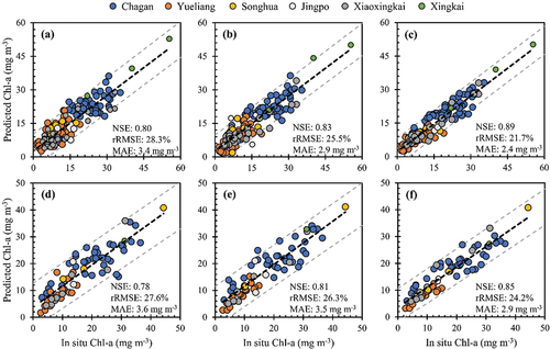
Among the three ML algorithms, the SVR-based model outperformed the other two, as indicated by the highest NSE of 0.89/0.85, the smallest rRMSE of 21.7%/24.2%, and the smallest MAE of 2.4/2.9 mg m⁻³ for the training/validation datasets (Figure 2), respectively. The paired t-test revealed no significant difference between the SVR-based Chl-a predictions and the in-situ measurements (Table S5). In addition to the overall performance, the SVR-based model also produced a generally consistent statistical distribution pattern with the in-situ measurements (Fig. S3(a)), and the smallest estimate errors in different Chl-a ranges (i.e. <10, 10–20, 20–30, and >30 mg m⁻³ in Fig. S3(b) and (c)). Indeed, SVR is generally considered to have better generalization capabilities when dealing with limited quantity and/or quality of training data. This further strengthens its advantages in water color monitoring cases, given the inadequacy of ground measurements (Mohebzadeh et al. 2021; Sun, Li, and Wang 2009). Despite the low Chl-a concentrations (<10 mg m⁻³) having relatively higher estimate errors (36.9% in Fig. S2), such precision level is acceptable referring to the objective of the Ocean Color Satellite Mission in Chl-a monitoring (i.e. an uncertainty level of 35%) (Moore, Campbell, and Dowell 2009). Also, compared to previous studies, such performance could be at least satisfactory (Guan et al. 2020; Li et al. 2021; Tilstone et al. 2021). Thus, the SVR-based model is capable of deriving the long-term Chl-a predictions for the NPLR lakes.

4.2. Long-term Chl-a change patterns in the NPLR lakes

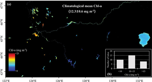
The SVR-based Chl-a model was applied to MERIS and OLCI observations to generate the long-term Chl-a maps from 2003 to 2011 and 2016 to 2019. The climatological mean values of Chl-a are displayed in Figure 3, and the Chl-a statistics of the examined lakes are summarized in Table S5. The Chl-a of NPLR lakes were found to vary spatially, with climatological mean values ranging from 6.8 mg m⁻³ (Mopanshan Reservoir) to 18.6 mg m⁻³ (Lake Kuli), averaging at 12.3 mg m⁻³. Nearly half of the lakes had an annual mean Chl-a concentration between 10 and 15 mg m⁻³, and 10 and 8 lakes were detected with an annual mean Chl-a lower than 10 mg m⁻³ and greater than 15 mg m⁻³, respectively (Figure 3(b)). In general, lakes distributed in the middle to lower reaches of the Nen River were found to have higher Chl-a concentrations (14.3 mg m⁻³ on average) compared to those in the mountainous area (7.9 mg m⁻³ on average, lakes with asterisks in Figure 1). Meanwhile, the Chl-a concentration was relatively higher in natural lakes than in reservoirs (13.8 versus 10.4 mg m⁻³ on average).

Figure 3. (a) is the long-term mean Chl-a concentration of the examined lakes in NPLR based on MERIS (2003–2012) and OLCI (2016–2019) observations; (b) shows the number of studied lakes in different annual mean Chl-a concentration categories.

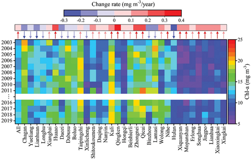
Figure 4 depicts the climatological annual mean Chl-a and the change rate for each lake during the study period. Overall, the NPLR lakes experienced a statistically significant increasing trend of 0.10 mg m⁻³/year. The change rate of lakes ranged from −0.21 (Lake Hulan) to 0.32 mg m⁻³/year (Lake Qingken). Specifically, 11 lakes had statistically significant increasing trends of Chl-a (p < 0.05, annotated with deep red upward arrows in Figure 4), and 3 lakes showed statistically significant decreasing trends of Chl-a, i.e. Lakes Chagan, Lianhuan, and Hulan (annotated with deep blue downward arrows in Figure 4). Spatially, the lakes with decreasing Chl-a were mainly distributed in the middle to lower reaches of the Nen River, while those with increasing Chl-a were primarily found in the mountainous area.

Figure 4. Annual mean Chl-a concentration for all examined lakes. Each column represents a lake, and each cell represents the annual mean Chl-a value. The upward arrows represent increasing trends (statistically nonsignificant results with p > 0.05 are in light red, and significant ones with p < 0.05 are in deep red), and the downward arrows represent decreasing trends (nonsignificant and significant results are respectively in light blue and deep blue).

In terms of intra-annual changes, the seasonality of Chl-a can be observed in NPLR lakes (Fig. S4), where higher Chl-a concentrations were found in the warm season (e.g. June to September), and lower Chl-a concentrations mainly occurred in the cold period (e.g. April and November).

4.3. Analysis of potential driving forces on interannual Chl-a changes

The correlations between annual mean Chl-a and seven corresponding explanatory variables are analyzed for each individual lake to explore the forcing factors of interannual Chl-a variations (Table 1). More than 80% of the lakes were detected to be significantly correlated to at least one factor, indicating a sufficient ability of the examined factors to explain Chl-a variations in NPLR lakes.

Results indicated that Chl-a in almost all lakes correlated positively to air temperature, while both positive and negative correlations were obtained between Chl-a and wind (in respective 14 and 19 lakes), precipitation (in respective 19 and 14 lakes), and runoff (in both 13 lakes). It appears that runoff was the most dominant factor among the hydro-climatic factors, which obtained statistically significant correlations with Chl-a in 10 lakes (6 positive correlations and 4 negative correlations, Figure 5), with r ranging from −0.55 to 0.74 (Table 1). In addition, Chl-a showed significant correlations with the annual mean air temperature, wind speed, and precipitation in 3 lakes, 7 lakes, and 4 lakes, respectively. Time-windowed correlation analyses between the Chl-a and hydro-climatic factors were performed on a monthly scale. As shown in Fig. S5, air temperature had significant positive effects on the monthly variation of Chl-a in general, and wind speed also provided notable negative effects in certain periods.

Figure 5. The interannual changes in annual mean Chl-a (black dot lines) and runoff (grey dot lines) for individual lakes that had statistically significant (p<0.05) correlations between them. The shaded gray area represents the observational gap between MERIS and OLCI.

Compared to air temperature, wind, precipitation, and runoff, the impacts of point source and non-point source loadings on Chl-a were found to be more pronounced. Agriculture fertilizer was found to be the most influential factor, with significant positive correlations found in 12 lakes (Figure 6), followed by livestock excrement and wastewater discharge, each of which exhibited significant correlations with Chl-a in 8 lakes (Figures 7 and 8).

Figure 6. The interannual changes in annual mean Chl-a (black dot lines) and fertilizer amount (grey dot lines) for individual lakes where statistically significant (p<0.05) positive correlations were found between them. The shaded gray area represents the observational gap between MERIS and OLCI.

Figure 7. The interannual changes in annual mean Chl-a (black dot lines) and livestock excrement amount (grey dot lines) for individual lakes where statistically significant (p<0.05) correlations were found between them. The shaded gray area represents the observational gap between MERIS and OLCI.

Figure 8. The interannual changes in annual mean Chl-a (black dot lines) and wastewater discharge (grey dot lines) for individual lakes where statistically significant (p<0.05) correlations were found between them. The shaded gray area represents the observational gap between MERIS and OLCI.

Furthermore, the GLM analysis was conducted to quantify the relative importance of each explanatory variable to the interannual dynamics of Chl-a. As shown in Figure 9, for all studied lakes, the seven examined factors accounted for 63.9% to 99.4% of the Chl-a variations, with 26 lakes obtaining a total relative importance exceeding 80%. Among the 33 studied lakes, agriculture fertilizer was the dominant factor, accounting for 18.9% on average of Chl-a changes. Runoff had an explanatory power of 16.2% on average, followed by livestock excrement (13.8%) and wastewater discharge (12.3%). Air temperature, wind, and precipitation played less important roles in altering the interannual Chl-a changes, with the relative importance of 11.3%, 7.1%, and 11.9% on average, respectively. Among the 22 lakes with increasing Chl-a, agriculture fertilizer was found to have statistically significant impacts in 10 lakes, with the most considerable explanatory power up to 65.9% in Lake Xiaoxingkai. Runoff was found to be the dominant explanatory factor of 7 lakes, accounting for 19.0% to 62.3% of the Chl-a increase, and wastewater discharge significantly accounted for more than 30% in 3 lakes. As for the 11 lakes with decreasing Chl-a, more than half of them were closely related to the decrease in livestock excrement (Figures 4 and 9).

Figure 9. Relative importance of the seven explanatory variables to the interannual Chl-a changes for each of the examined lakes, where “*” denotes a statistically significant result with p<0.05. The black and red hollow boxes are the total relative importance of hydro-climatic factors and anthropogenic factors.

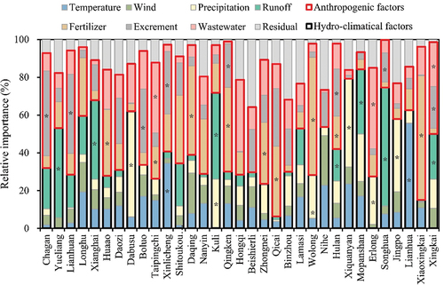
The red and black hollow boxes in Figure 9 added the relative importance of explanatory variables in terms of the hydro-climatic and anthropogenic factors, respectively. In general, anthropogenic factors explained most of the variability of interannual Chl-a changes in NPLR lakes and acted as the dominant driving forces. The total relative importance of the three anthropogenic factors exceeded 50% in 18 lakes, while the prominent influence of hydro-climatic factors was detected in 12 lakes, accounting for more than 50% of the long-term Chl-a changes. It is found that lakes significantly influenced by anthropogenic activities (with more than 50% explanatory power for Chl-a changes) are mostly distributed in plain regions, while lakes in mountainous regions appeared to be more susceptible to hydro-climatic factors.

5. Discussion

5.1. Uncertainties of the estimated Chl-a concentration

Due to the complex optical environment of coastal and inland waters, the uncertainties of atmospheric correction (AC) in deriving surface reflectance remain a challenge in water environment monitoring by remote sensing means (Vanhellemont and Ruddick 2021; Warren, Simis, and Selmes 2021). This study adopted the POLYMER algorithm to generate the surface reflectance from top-of-atmospheric radiance detected by MERIS and OLCI instruments. Initially developed for MERIS data, POLYMER has shown superior abilities in obtaining accurate surface reflectance in turbid case-II waters, not only in terms of the rationality of the spectra derived (Guan et al. 2020) but also in the quantity of the valid R_rs data obtained under unfavorable observation conditions (Zhang et al. 2018). Nowadays, POLYMER has been extended to many other sensors, including OLCI, and applied to global water color monitoring as an effective processor (Giannini et al. 2021; Mograne et al. 2019). In this study, the short-wavelength bands (e.g. the blue bands), which are often associated with considerable uncertainties, were excluded from the Chl-a retrieval (Zhang et al. 2018). Moreover, the concurrent satellite R_rs was directly used to establish the Chl-a retrieval model, suggesting that the uncertainties of AC-corrected R_rs would be implicitly compensated during the fitting process of model construction. Thus, the uncertainties in R_rs will have a very limited impact on the long-term estimation and interpretation of Chl-a.

As mentioned above, observations from two satellite instruments (i.e. MERIS and OLCI) were applied in this study. Ideally, match-ups of both instruments should be collected for Chl-a model construction to avoid the effect of cross-sensor variability. However, due to the absence of field measurements during the MERIS period, only the OLCI match-ups were used to establish the retrieval model, which may cause uncertainties in Chl-a retrievals during the MERIS period. Fortunately, as a successor to the MERIS mission, OLCI shared multiple similarities with MERIS in terms of spatial, spectral, and radiometric characteristics (Liu et al. 2018; Smith, Robertson Lain, and Bernard 2018). This suggests that the two approaches have comparable observational capability. Several studies have also demonstrated a strong consistency in water environment monitoring between these two products (Liu et al. 2018; Pastor-Guzman et al. 2020; Smith, Robertson Lain, and Bernard 2018). For example, Guan et al. (2020) compared the Chl-a concentrations derived from the equivalent R_rs of MERIS and OLCI (converted from the field measurements) and observed a good agreement between the estimations from the two products across the Yangtze Plain in southern China. Based on this evidence, this study further showed satisfactory performances of the Chl-a algorithm for both sensors, and the diverged Chl-a change trends (higher or lower) between two observation periods are different among lakes, e.g. Chl-a during the MERIS period was found to be higher than that during the OLCI period of Lakes Chagan, Lianhuan, and Hulan, etc., while the reverse was true for Lakes Songhua, Jingpo, and Qingken, etc. Such trends would not happen in the presence of significant systematic errors between MERIS and OLCI observations. As stated above, the cross-sensors could not lead to significant systematic errors in the long-term Chl-a monitoring in NPLR lakes and the validity of the Chl-a estimation could be justified.

An ML-based (i.e. SVR) algorithm was developed for Chl-a retrievals in NPLR lakes. Despite that the ML approaches have shown unparalleled advantages over traditional mathematical methods in mining complex relationships between reflectance and Chl-a concentrations (Table 2), they should be prudently applied in the practice of water quality monitoring because these models rely heavily on the data quantity and quality for model training and the structures of ML algorithms (Kotsiantis, Zaharakis, and Pintelas 2007). In this study, 237 match-ups covering a wide range of Chl-a concentrations (1.7–55.4 mg m⁻³) were used to establish the retrieval model; such a range of measurements could be able to represent the dynamic variation of interannual and intra-annual Chl-a in NPLR as documented by previous studies (Duan et al. 2007; Guo et al. 2018; Li et al. 2016). Additionally, the training datasets contained low to high concentrations of Chl-a measurements and match-ups from all the sampled lakes, ensuring that the ML-based models could learn enough information during the model training process (Figure 2). Furthermore, this study compared the capabilities of various ML algorithms in Chl-a prediction, and the SVR-based model was then selected because it produced superior performances in both training and validation datasets (NSE >0.85, rRMSE < 25%, and MAE <3.0 mg m⁻³), being adequately practical for the long-term Chl-a monitoring.

The presence of apparent surface phytoplankton scums (when phytoplankton float at the surface under severe phytoplankton blooms) or aquatic vegetation could contaminate the satellite signals because they have stronger reflections than water areas (Kravitz et al. 2020), which thus would impact the retrieval of Chl-a concentration. It is fortunate that the pixels covered with such phytoplankton scums or vegetation were flagged during the AC process using POLYMER algorithm, and no R_rs will be generated for such pixels. In this context, the estimated Chl-a concentrations in this study were less contaminated by surface phytoplankton scums or vegetation. It should also be noted that neglecting the Chl-a concentration of these pixels may result in an underestimation of phytoplankton biomass. However, surface scums in NPLR lakes have rarely been observed by Landsat at 30 m resolution (Fang et al. 2018), let alone by the MERIS and OLCI observations with ten times coarser resolution. As such, the influence of surface scums on Chl-a statistics in this study should be minimum (at least from the perspective of MERIS and OLCI products).

5.2. Implications for managing human-induced eutrophication in NPLR lakes

Chl-a provides a reasonable estimate of phytoplankton (referring to free-floating phytoplankton) biomass (Carlson 1977), and the phytoplankton growth rate is controlled by various environmental variables, including temperature, water movement, nutrients, and light. The hydro-climatic factors and anthropogenic activities can alter these environmental variables of lakes in different ways, which in turn affect phytoplankton growth rate and biomass. This study demonstrated that anthropogenic activities were the primary drivers (total relative importance > 50%, Section 4.2) of the long-term Chl-a changes in more than half of the examined lakes. Understanding the causal effects between the Chl-a concentration and anthropogenic activities can serve as the baseline information for policy-makers to propose sustainable management solutions.

According to the statistics of Jilin and Heilongjiang Provinces, the annual chemical fertilizer usage has rapidly increased by more than 45% from 2003 to 2019 (Fig. S6). The continual increase in fertilizer application was found to be significantly correlated with Chl-a increase in 12 lakes (Table 1) and play a statistically significant role in affecting the Chl-a variations of 9 lakes (Figure 9). Livestock excrement was found to serve as a major explanatory factor to Chl-a changes in 7 examined lakes because animal feedlots were hardly treated before being drained into the water body in rural areas. Apart from non-point source pollution, the impacts from point source pollution (i.e. industrial wastewater discharge) should also be noted in several lakes (e.g. Lakes Hulan, Erlong, and Hongqi) (Figure 7).

The loss of non-point source pollution into lakes is strongly associated with surface runoff. Though runoff was counted as a hydro-climatic factor in this study, the roles of runoff in affecting the Chl-a concentration of lakes were diverged. On one hand, runoff replenishment can contribute to diluting the pollutant concentrations of lakes (e.g. Xianghai, Xinlicheng, and Shitoukoumen Reservoirs). On the other hand, runoff scours the drainage area, carrying nutrients into lakes, especially in lake catchments with intense non-point source pollution (e.g. Lakes Chagan, Songhua and Xiaoxingkai) (Liu et al. 2021, 2011; Yang et al. 2010). Wind was found to significantly regulate Chl-a changes in 7 lakes (Table 1). Nutrients settled to the bottom can be resuspended into the water column triggered by wind forcing in shallow lakes (Ji and Jin 2006) and subsequently fuel the algae bloom. However, this resuspension can also diminish the euphotic zone and light availability for algae growth.

In addition to the long-term Chl-a changes, seasonal variations of Chl-a were also noted, with a higher Chl-a concentration in warm seasons and a lower Chl-a concentration in cold periods. As phytoplankton growth rate increases with temperature until an optimum is reached (USEPA 2000), the rising temperature in summer most likely promoted the growth of cyanobacteria in NPLR lakes, resulting in a high concentration of Chl-a in summer.

This study provided a high-quality Chl-a record and a comprehensive insight into the influencing mechanisms of Chl-a variations of basin-scale lakes in the Northeast Plains-Mountain Lake Region. The analytical framework can be referable and extendable to other similar inland and coastal regions with densely distributed lakes for tracing the long-term water quality dynamics. In this study, the primary stressors related to Chl-a changes were found to vary among lakes. Therefore, river basin management strategies should be tailored for each water body. For example, optimizing fertilization is a practical way to reduce agricultural non-point source pollution, and the centralized wastewater treatment systems should be equipped for the scattered and concentrated animal feedlots.

The seven explanatory factors examined in this study can effectively interpret the Chl-a dynamics in most lakes, with the total relative importance exceeding 80% in 26 lakes. In the case of the four hydro-climatic factors, it’s noted that some recording stations are located at a certain distance from the lakes. Given the high spatial resolution data, further validation of their impacts on Chl-a dynamics is still necessary. Furthermore, this study focused exclusively on three human-induced factors, namely agriculture fertilizer, livestock excrement, and wastewater discharge. It is important to recognize that there are other factors influencing phytoplankton growth in lakes, such as the economic activities of lakes (i.e. fishing, leisure, and tourism industries) (Li et al. 2022; Liu et al. 2019; Su, Wall, and Ma 2014; Yu et al. 2021), and the regulatory regimes of central or local government (Gao et al. 2023; Qin et al. 2020). In addition to the factors addressed in this study, enhanced analysis of the potential influences of multiple forces would contribute to a better understanding of the Chl-a changing mechanisms in lakes, especially for those with relatively weak interpretability (e.g. Lakes Beishierli, Binzhou, Lamasi, and Nihe Reservoir, with the residual relative importance of more than 20%).

This study revealed the statistical correlation between environmental variables and Chl-a concentrations; however, the Chl-a concentration and lake eutrophication status are highly related to complex hydro-chemical and biological processes. Phytoplankton biomass is governed by phytoplankton growth, metabolism (including respiration and excretion), predation, settling, and external sources (Ji 2017). Among these processes, phytoplankton growth is the most important factor influencing phytoplankton biomass and is a multiplicative function of temperature, light, and nutrients. With sufficient hydrological, environmental, and ecological data, future investigations can delve deeper into the mechanisms governing phytoplankton kinetics in lakes based on numerical/physical models.

6. Conclusions

This study successfully developed and applied a practical SVR-based model to establish Chl-a data records for 33 lakes (>15 km²) in the NPLR using MERIS and OLCI observations between 2003 and 2019. The long-term retrievals revealed the Chl-a change rates ranging from −0.21 to 0.32 mg m⁻³/year across the lakes. Among them, 11 lakes exhibited statistically significant increasing trends, while 3 lakes showed significantly decreasing trends. Spatially, lakes in the mountainous region and east plain region generally exhibited increasing trends of Chl-a, while those in the middle to lower reaches of the Nen River experienced decreased Chl-a values. Furthermore, this study identified the driving forces behind interannual Chl-a changes, highlighting the significant influences of both hydro-climatic factors and anthropogenic activities. Non-point source pollution, particularly agriculture fertilizer and livestock excrement, were found to be the most important anthropogenic factors impacting Chl-a dynamics in lakes. This emphasized the need to address non-point source pollution associated with agricultural activities for economically and ecologically sustainable development in northeastern China.

To the best of our knowledge, this is the first comprehensive assessment of Chl-a changes over broad spatial and temporal scales across the NPLR lakes. The results provide valuable insights into the dynamics and influencing factors of Chl-a in the NPLR lakes, contributing to the understanding and management of human-induced eutrophication in the region. Moreover, the developed SVR-based model for Chl-a prediction holds promise as a candidate model for near real-time remote sensing monitoring of Chl-a using OLCI observations. However, further research is warranted to delve deeper into the complex hydro-chemical and biological processes governing Chl-a dynamics and improve the accuracy of Chl-a estimations through advanced modeling approaches.

Highlights

• Runoff was the second most important stressor for inter-annual Chl-a changes in NPLR

• A machine learning-based algorithm was developed for retrieving Chl-a of inland lakes

• Long-term Chl-a dynamics in NPLR lakes were revealed using MERIS and OLCI data

• Increasing fertilizer application primarily contributed to Chl-a increases in 12 lakes

Author contributions

Lu Zhang: Methodology, Formal analysis, Writing – Original Draft. Zhuohang Xin: Conceptualization, Writing – Review & Editing, Funding acquisition. Qi Guan: Methodology. Lian Feng: Supervision, Writing – Review & Editing. Chuanmin Hu: Supervision, Writing – Review & Editing. Chi Zhang: Funding acquisition. Huicheng Zhou: Supervision, Funding acquisition.

Acknowledgments

This research was supported by the National Natural Science Foundation of China [grant numbers 51925902, U21A20155, 52279007]. We gratefully acknowledge NASA for providing MERIS and OLCI surface reflectance. We also thank the reviewers for their constructive suggestions.

Disclosure statement

The authors declare that they have no known competing financial interests or personal relationships that could have appeared to influence the work reported in this paper.

Data availability statement

The MERIS and OLCI reflectance data used in this study can be accessed through the NASA Goddard Space Flight Center (http://oceancolor.gsfc.nasa.gov/cgi/browse.pl?sen=amod). The climatic records were available at http://data.cma.cn/data/cdcdetail/dataCode/SURF_CLI_CHN_MUL_MMON_19812010.html. The annual fertilizer application amount, livestock population, and wastewater discharge amount can be obtained through http://data.cnki.net/Yearbook.

Supplementary material

Supplemental data for this article can be accessed online at https://doi.org/10.1080/15481603.2023.2285166.

Additional information

Funding

The work was supported by the National Natural Science Foundation of China [52279007, 51925902, U21A20155].

References

- Ahlgren, P., and B. Jarneving. 2003. “Requirements for a Cocitation Similarity Measure, with Special Reference to Pearson’s Correlation Coefficient.” Journal of the American Society for Information Science and Technology 54 (6): 550–19. https://doi.org/10.1002/asi.10242.
- Aptoula, E., and S. Ariman. 2021. “Chlorophyll-A Retrieval from Sentinel-2 Images Using Convolutional Neural Network Regression.” IEEE Geoscience and Remote Sensing Letters 19:1–5. https://doi.org/10.1109/LGRS.2021.3070437.
- Attila, J., P. Kauppila, K. Y. Kallio, H. Alasalmi, V. Keto, E. Bruun, and S. Koponen. 2018. “Applicability of Earth Observation Chlorophyll-A Data in Assessment of Water Status via MERIS — with Implications for the Use of OLCI Sensors.” Remote Sensing of Environment 212:273–287. https://doi.org/10.1016/j.rse.2018.02.043.
- Bao, W., Y. Yang, T. Fu, and G. H. Xie. 2019. “Estimation of Livestock Excrement and Its Biogas Production Potential in China.” Journal of Cleaner Production 229:1158–1166. https://doi.org/10.1016/j.jclepro.2019.05.059.
- Binding, C. E., T. A. Greenberg, and R. P. Bukata. 2011. “Time Series Analysis of Algal Blooms in Lake of the Woods Using the MERIS Maximum Chlorophyll Index.” Journal of Plankton Research 33 (12): 1847–1852. https://doi.org/10.1093/plankt/fbr079.
- Cannizzaro, J. P., and K. L. Carder. 2006. “Estimating Chlorophyll a Concentrations from Remote-Sensing Reflectance in Optically Shallow Waters.” Remote Sensing of Environment 101 (1): 13–24. https://doi.org/10.1016/j.rse.2005.12.002.
- Carlson, R. E. 1977. “A Trophic State Index for Lakes.” Limnology and Oceanography 22 (2): 361–369. https://doi.org/10.4319/lo.1977.22.2.0361.
- Chen, Q., M. Huang, and X. Tang. 2020. “Eutrophication Assessment of Seasonal Urban Lakes in China Yangtze River Basin Using Landsat 8-Derived Forel-Ule Index: A Six-Year (2013-2018) Observation.” Science of the Total Environment 745:135392. https://doi.org/10.1016/j.scitotenv.2019.135392.
- Dall’olmo, G., and A. A. Gitelson. 2005. “Effect of Bio-Optical Parameter Variability on the Remote Estimation of Chlorophyll-A Concentration in Turbid Productive Waters: Experimental Results.” Applied Optics 44 (3): 412–422. https://doi.org/10.1364/AO.44.000412.
- Duan, H., R. Ma, X. Xu, F. Kong, S. Zhang, W. Kong, J. Hao, and L. Shang. 2009. Two-Decade Reconstruction of Algal Blooms in China’s Lake Taihu 43 (10): 3522–3528. https://doi.org/10.1021/es8031852.
- Duan, H., Y. Zhang, B. Zhang, K. Song, Z. Wang, D. Liu, and F. Li. 2007. “Estimation of Chlorophyll-A Concentration and Trophic States for Inland Lakes in Northeast China from Landsat TM Data and Field Spectral Measurements.” International Journal of Remote Sensing 29 (3): 767–786. https://doi.org/10.1080/01431160701355249.
- Du, Y., K. Song, G. Liu, Z. Wen, C. Fang, Y. Shang, F. Zhao, Q. Wang, J. Du, and B. Zhang. 2020. “Quantifying Total Suspended Matter (TSM) in Waters Using Landsat Images During 1984-2018 Across the Songnen Plain, Northeast China.” Journal of Environmental Management 262:110334. https://doi.org/10.1016/j.jenvman.2020.110334.
- Fang, C., K. Song, L. Li, Z. Wen, G. Liu, J. Du, Y. Shang, and Y. Zhao. 2018. “Spatial Variability and Temporal Dynamics of HABs in Northeast China.” Ecological Indicators 90:280–294. https://doi.org/10.1016/j.ecolind.2018.03.006.
- Feng, L., X. Hou, and Y. Zheng. 2019. “Monitoring and Understanding the Water Transparency Changes of Fifty Large Lakes on the Yangtze Plain Based on Long-Term MODIS Observations.” Remote Sensing of Environment 221:675–686. https://doi.org/10.1016/j.rse.2018.12.007.
- Feng, L., C. Hu, X. Han, X. Chen, and L. Qi. 2014. “Long-Term Distribution Patterns of Chlorophyll-A Concentration in China’s Largest Freshwater Lake: MERIS Full-Resolution Observations with a Practical Approach.” Remote Sensing 7 (1): 275–299. https://doi.org/10.3390/rs70100275.
- François, S., D. Pierre-Yves, and R. Didier. 2011. “Atmospheric Correction in Presence of Sun Glint: Application to MERIS.” Optics Express 19 (10): 9783–9800. https://doi.org/10.1364/OE.19.009783.
- Gao, J., G. Deng, H. Jiang, Y. Wen, S. Zhu, C. He, C. Shi, and Y. Cao. 2023. “Water Quality Pollution Assessment and Source Apportionment of Lake Wetlands: A Case Study of Xianghai Lake in the Northeast China Plain.” Journal of Environmental Management 344:118398. https://doi.org/10.1016/j.jenvman.2023.118398.
- García-Nieto, P. J., E. García-Gonzalo, J. R. Alonso Fernández, and C. Díaz Muñiz. 2020. “A New Predictive Model for Evaluating Chlorophyll-A Concentration in Tanes Reservoir by Using a Gaussian Process Regression.” Water Resources Management 34 (15): 4921–4941. https://doi.org/10.1007/s11269-020-02699-x.
- Giannini, F., B. P. V. Hunt, D. Jacoby, and M. Costa. 2021. “Performance of OLCI Sentinel-3A Satellite in the Northeast Pacific Coastal Waters.” Remote Sensing of Environment 256:112317. https://doi.org/10.1016/j.rse.2021.112317.
- Gitelson, A. A., G. Dall’olmo, W. Moses, D. C. Rundquist, T. Barrow, T. R. Fisher, D. Gurlin, and J. Holz. 2008. “A Simple Semi-Analytical Model for Remote Estimation of Chlorophyll-A in Turbid Waters: Validation.” Remote Sensing of Environment 112 (9): 3582–3593. https://doi.org/10.1016/j.rse.2008.04.015.
- Gower, J. F. R., R. Doerffer, and G. A. Borstad. 2010. “Interpretation of the 685 Nm Peak in Water-Leaving Radiance Spectra in Terms of Fluorescence, Absorption and Scattering, and Its Observation by MERIS.” International Journal of Remote Sensing 20 (9): 1771–1786. https://doi.org/10.1080/014311699212470.
- Gower, J., S. King, G. Borstad, and L. Brown. 2005. “Detection of Intense Plankton Blooms Using the 709 nm Band of the MERIS Imaging Spectrometer.” International Journal of Remote Sensing 26 (9): 2005–2012. https://doi.org/10.1080/01431160500075857.
- Guan, Q., L. Feng, X. Hou, G. Schurgers, Y. Zheng, and J. Tang. 2020. “Eutrophication Changes in Fifty Large Lakes on the Yangtze Plain of China Derived from MERIS and OLCI Observations.” Remote Sensing of Environment 246:111890. https://doi.org/10.1016/j.rse.2020.111890.
- Guo, J., C. Zhang, G. Zheng, J. Xue, and L. Zhang. 2018. “The Establishment of Season-Specific Eutrophication Assessment Standards for a Water-Supply Reservoir Located in Northeast China Based on Chlorophyll-A Levels.” Ecological Indicators 85:11–20. https://doi.org/10.1016/j.ecolind.2017.09.056.
- Han, X., L. Feng, X. Chen, and H. Yesou. 2014. “MERIS Observations of Chlorophyll-A Dynamics in Erhai Lake Between 2003 and 2009.” International Journal of Remote Sensing 35 (24): 8309–8322. https://doi.org/10.1080/01431161.2014.985395.
- He, J., Y. Chen, J. Wu, D. A. Stow, and G. Christakos. 2020. “Space-Time Chlorophyll-A Retrieval in Optically Complex Waters That Accounts for Remote Sensing and Modeling Uncertainties and Improves Remote Estimation Accuracy.” Water Research 171:115403. https://doi.org/10.1016/j.watres.2019.115403.
- Ho, J. C., A. M. Michalak, and N. Pahlevan. 2019. “Widespread Global Increase in Intense Lake Phytoplankton Blooms Since the 1980s.” Nature 574 (7780): 667–670. https://doi.org/10.1038/s41586-019-1648-7.
- Hsu, C. W., C. C. Chang, and C. J. Lin. 2003. A Practical Guide to Support Vector Classification. Taipei. Accessed February 21, 2021. https://www.csie.ntu.edu.tw/~cjlin/papers/guide/guide.pdf.
- Huovinen, P., J. Ramirez, L. Caputo, and I. Gomez. 2019. “Mapping of Spatial and Temporal Variation of Water Characteristics Through Satellite Remote Sensing in Lake Panguipulli, Chile.” Science of the Total Environment 679:196–208. https://doi.org/10.1016/j.scitotenv.2019.04.367.
- Ji, Z.-G. 2017. Hydrodynamics and Water Quality: Modeling Rivers, Lakes, and Estuaries. America: John Wiley & Sons.
- Jiang, G., S. A. Loiselle, D. Yang, R. Ma, W. Su, and C. Gao. 2020. “Remote Estimation of Chlorophyll a Concentrations Over a Wide Range of Optical Conditions Based on Water Classification from VIIRS Observations.” Remote Sensing of Environment 241:241. https://doi.org/10.1016/j.rse.2020.111735.
- Ji, Z.-G., and K.-R. Jin. 2006. “Gyres and Seiches in a Large and Shallow Lake.” Journal of Great Lakes Research 32 (4): 764–775. https://doi.org/10.3394/0380-1330(2006)32[764:GASIAL]2.0.CO;2.
- Kotsiantis, S. B., I. D. Zaharakis, and P. E. Pintelas. 2007. “Machine Learning: A Review of Classification and Combining Techniques.” Artificial Intelligence Review 26 (3): 159–190. https://doi.org/10.1007/s10462-007-9052-3.
- Kravitz, J., M. Matthews, S. Bernard, and D. Griffith. 2020. “Application of Sentinel 3 OLCI for Chl-A Retrieval Over Small Inland Water Targets: Successes and Challenges.” Remote Sensing of Environment 237:237. https://doi.org/10.1016/j.rse.2019.111562.
- Li, Z., Z. Jiang, Y. Qu, Y. Cao, F. Sun, and Y. Dai. 2022. “Analysis of Landscape Change and Its Driving Mechanism in Chagan Lake National Nature Reserve.” Sustainability 14 (9): 5675. https://doi.org/10.3390/su14095675.
- Li, S., K. Song, G. Mu, Y. Zhao, J. Ma, and J. Ren. 2016. “Evaluation of the Quasi-Analytical Algorithm (QAA) for Estimating Total Absorption Coefficient of Turbid Inland Waters in Northeast China.” IEEE Journal of Selected Topics in Applied Earth Observations and Remote Sensing 9 (9): 4022–4036. https://doi.org/10.1109/JSTARS.2016.2549026.
- Li, S., K. Song, S. Wang, G. Liu, Z. Wen, Y. Shang, L. Lyu, et al. 2021. “Quantification of Chlorophyll-A in Typical Lakes Across China Using Sentinel-2 MSI Imagery with Machine Learning Algorithm.” Science of the Total Environment 778:146271. https://doi.org/10.1016/j.scitotenv.2021.146271.
- Liu, Y., L. Li, L. Liang, and J. Li. 2011. “Study on the Non-Point Source Pollution in the Upper and Middle Reaches of the Taoer River Basin.” Chinese Journal of Population Resources and Environment 9 (1): 48–54. https://doi.org/10.1080/10042857.2011.10685018.
- Liu, G., S. G. H. Simis, L. Li, Q. Wang, Y. Li, K. Song, H. Lyu, Z. Zheng, and K. Shi. 2018. “A Four-Band Semi-Analytical Model for Estimating Phycocyanin in Inland Waters from Simulated MERIS and OLCI Data.” IEEE Transactions on Geoscience and Remote Sensing 56 (3): 1374–1385. https://doi.org/10.1109/TGRS.2017.2761996.
- Liu, D., C. Song, C. Fang, Z. Xin, J. Xi, and Y. Lu. 2021. “A Recommended Nitrogen Application Strategy for High Crop Yield and Low Environmental Pollution at a Basin Scale.” Science of the Total Environment 792:148464. https://doi.org/10.1016/j.scitotenv.2021.148464.
- Liu, R., J. Wang, J. Shi, Y. Chen, C. Sun, P. Zhang, and Z. Shen. 2014. “Runoff Characteristics and Nutrient Loss Mechanism from Plain Farmland Under Simulated Rainfall Conditions.” Science of the Total Environment 468-469:1069–1077. https://doi.org/10.1016/j.scitotenv.2013.09.035.
- Liu, X., G. Zhang, G. Sun, Y. Wu, and Y. Chen. 2019. “Assessment of Lake Water Quality and Eutrophication Risk in an Agricultural Irrigation Area: A Case Study of the Chagan Lake in Northeast China.” Water 11 (11): 2380. https://doi.org/10.3390/w11112380.
- Matthews, M. W., S. Bernard, and K. Winter. 2010. “Remote Sensing of Cyanobacteria-Dominant Algal Blooms and Water Quality Parameters in Zeekoevlei, a Small Hypertrophic Lake, Using MERIS.” Remote Sensing of Environment 114 (9): 2070–2087. https://doi.org/10.1016/j.rse.2010.04.013.
- MEP. 2002. Environmental Quality Standards for Surface Water (GB 3838–2002) (In Chinese). https://www.mee.gov.cn/ywgz/fgbz/bz/bzwb/shjbh/shjzlbz/200206/W020061027509896672057.pdf.
- Mishra, D. R., B. A. Schaeffer, and D. Keith. 2014. “Performance Evaluation of Normalized Difference Chlorophyll Index in Northern Gulf of Mexico Estuaries Using the Hyperspectral Imager for the Coastal Ocean.” GIScience & Remote Sensing 51 (2): 175–198. https://doi.org/10.1080/15481603.2014.895581.
- Mograne, M., C. Jamet, H. Loisel, V. Vantrepotte, X. Mériaux, and A. Cauvin. 2019. “Evaluation of Five Atmospheric Correction Algorithms Over French Optically-Complex Waters for the Sentinel-3A OLCI Ocean Color Sensor.” Remote Sensing 11 (6): 668. https://doi.org/10.3390/rs11060668.
- Mohebzadeh, H., E. Mokari, P. Daggupati, and A. Biswas. 2021. “A Machine Learning Approach for Spatiotemporal Imputation of MODIS Chlorophyll a.” International Journal of Remote Sensing 42 (19): 7381–7404. https://doi.org/10.1080/01431161.2021.1957513.
- Moore, T. S., J. W. Campbell, and M. D. Dowell. 2009. “A Class-Based Approach to Characterizing and Mapping the Uncertainty of the MODIS Ocean Chlorophyll Product.” Remote Sensing of Environment 113 (11): 2424–2430. https://doi.org/10.1016/j.rse.2009.07.016.
- Moses, W. J., A. A. Gitelson, S. Berdnikov, and V. Povazhnyy. 2009. “Satellite Estimation of Chlorophyll-A Concentration Using the Red and NIR Bands of MERIS—The Azov Sea Case Study.” IEEE Geoscience and Remote Sensing Letters 6 (4): 845–849. https://doi.org/10.1109/LGRS.2009.2026657.
- Mueller, J. L., A. Morel, R. Frouin, C. Davis, R. Arnone, K. Carder, Z. Lee, R. Steward, S. Hooker, and C. Mobley. 2003. “Ocean optics protocols for satellite ocean color sensor validation, revision 4.” Volume III: Radiometric Measurements and Data Analysis Protocols. https://oceancolor.gsfc.nasa.gov/docs/technical/
- NIGLAS. 2019. National Lake Survey Report in China (In Chinese). Nanjing: Nanjing Institute of Geography and Limnology, Chinese Academy of Sciences.
- Pahlevan, N., S. K. Chittimalli, S. V. Balasubramanian, and V. Vellucci. 2019. “Sentinel-2/Landsat-8 Product Consistency and Implications for Monitoring Aquatic Systems.” Remote Sensing of Environment 220:19–29. https://doi.org/10.1016/j.rse.2018.10.027.
- Pastor-Guzman, J., L. Brown, H. Morris, L. Bourg, P. Goryl, S. Dransfeld, and J. Dash. 2020. “The Sentinel-3 OLCI Terrestrial Chlorophyll Index (OTCI): Algorithm Improvements, Spatiotemporal Consistency and Continuity with the MERIS Archive.” Remote Sensing 12 (16): 2652. https://doi.org/10.3390/rs12162652.
- Qin, G., J. Liu, S. Xu, and T. Wang. 2020. “Water Quality Assessment and Pollution Source Apportionment in a Highly Regulated River of Northeast China.” Environmental Monitoring and Assessment 192 (7): 446. https://doi.org/10.1007/s10661-020-08404-0.
- Smith, M. E., L. Robertson Lain, and S. Bernard. 2018. “An Optimized Chlorophyll a Switching Algorithm for MERIS and OLCI in Phytoplankton-Dominated Waters.” Remote Sensing of Environment 215:217–227. https://doi.org/10.1016/j.rse.2018.06.002.
- Sun, D., Y. Li, and Q. Wang. 2009. “A Unified Model for Remotely Estimating Chlorophyll a in Lake Taihu, China, Based on SVM and in situ Hyperspectral Data.” IEEE Transactions on Geoscience and Remote Sensing 47 (8): 2957–2965. https://doi.org/10.1109/TGRS.2009.2014688.
- Su, M. M., G. Wall, and Z. Ma. 2014. “Assessing Ecotourism from a Multi-Stakeholder Perspective: Xingkai Lake National Nature Reserve, China.” Environmental Management 54 (5): 1190–1207. https://doi.org/10.1007/s00267-014-0360-5.
- Tilstone, G. H., S. Pardo, G. Dall’olmo, R. J. W. Brewin, F. Nencioli, D. Dessailly, E. Kwiatkowska, T. Casal, and C. Donlon. 2021. “Performance of Ocean Colour Chlorophyll a Algorithms for Sentinel-3 OLCI, MODIS-Aqua and Suomi-VIIRS in Open-Ocean Waters of the Atlantic.” Remote Sensing of Environment 260:112444. https://doi.org/10.1016/j.rse.2021.112444.
- Tzortziou, M., A. Subramaniam, J. R. Herman, C. L. Gallegos, P. J. Neale, and L. W. Harding. 2007. “Remote Sensing Reflectance and Inherent Optical Properties in the Mid Chesapeake Bay.” Estuarine, Coastal and Shelf Science 72 (1–2): 16–32. https://doi.org/10.1016/j.ecss.2006.09.018.
- USEPA. 2000. “Chapter: The Basis for Lake and Reservoir Nutrient Criteria.“ In Nutrient Criteria Technical Guidance Manual-Lakes and Reservoirs, 1–16. Washington, DC: Office of water, office of science and technology.
- Vanhellemont, Q., and K. Ruddick. 2021. “Atmospheric Correction of Sentinel-3/OLCI Data for Mapping of Suspended Particulate Matter and Chlorophyll-A Concentration in Belgian Turbid Coastal Waters.” Remote Sensing of Environment 256:112284. https://doi.org/10.1016/j.rse.2021.112284.
- Wang, R., T. Xu, L. Yu, J. Zhu, and X. Li. 2013. “Effects of Land Use Types on Surface Water Quality Across an Anthropogenic Disturbance Gradient in the Upper Reach of the Hun River, Northeast China.” Environmental Monitoring and Assessment 185 (5): 4141–4151. https://doi.org/10.1007/s10661-012-2856-x.
- Warren, M. A., S. G. H. Simis, and N. Selmes. 2021. “Complementary Water Quality Observations from High and Medium Resolution Sentinel Sensors by Aligning Chlorophyll-A and Turbidity Algorithms.” Remote Sensing of Environment 265:112651. https://doi.org/10.1016/j.rse.2021.112651.
- Yang, W., B. Matsushita, J. Chen, T. Fukushima, and R. Ma. 2010. “An Enhanced Three-Band Index for Estimating Chlorophyll-A in Turbid Case-II Waters: Case Studies of Lake Kasumigaura, Japan, and Lake Dianchi, China.” IEEE Geoscience and Remote Sensing Letters 7 (4): 655–659. https://doi.org/10.1109/LGRS.2010.2044364.
- Yu, S., X. Li, B. Wen, G. Chen, A. Hartleyc, M. Jiang, and X. Li. 2021. “Characterization of Water Quality in Xiao Xingkai Lake: Implications for Trophic Status and Management.” CHINESE GEOGRAPHICAL SCIENCE 31 (3): 558–570. https://doi.org/10.1007/s11769-021-1199-3.
- Zhang, M., C. Hu, J. Cannizzaro, D. English, B. B. Barnes, P. Carlson, and L. Yarbro. 2018. “Comparison of Two Atmospheric Correction Approaches Applied to MODIS Measurements Over North American Waters.” Remote Sensing of Environment 216:442–455. https://doi.org/10.1016/j.rse.2018.07.012.