Fine-grained wetland classification for national wetland reserves using multi-source remote sensing data and Pixel Information Expert Engine (PIE-Engine)

ABSTRACT

Timely and accurate wetland information is necessary for wetland resource management. Recent advances in machine learning and remote sensing have facilitated cost-effective monitoring of wetlands. However, reliable methods for fine-grained and rapid wetland mapping are still lacking. To address the issue, a wetland sample set with 20 categories for China was collected based on a sampling strategy that combines automatic sample generation and visual interpretation. Simultaneously, a novel multi-stage method for fine-grained wetland classification was proposed, which integrates pixel-based and object-based strategies using ensemble learning algorithms and multi-source remote sensing data. First, a pixel-based ensemble learning algorithm was implemented to classify five rough wetland categories and six non-wetland categories. Second, an object-based ensemble learning approach was designed to separate the water cover in the pixel-based classification results into eight detailed categories. Third, the merged pixel-based and object-based classification results were refined with knowledge-based post-processing procedures to identify 14 fine-grained wetland categories. Results using the Pixel Information Expert Engine (PIE-Engine) cloud platform proved the effectiveness of the proposed wetland classification method. The overall accuracy, kappa, and weighted F1 reached 87.39%, 82.80%, and 86.02%, respectively. The adopted ensemble learning algorithm yielded better performance than classifiers such as CatBoost, random forest, and XGBoost. The incorporation of spectral, texture, shape, topographic, and geographic features from multi-source data contributed to differentiating wetland categories. According to the relative contribution, spectral indexes (NDVI and NDWI), texture features (sum average and contrast), and topographic features (slope and elevation) were identified as important leading predictors for the first-stage pixel-based classification. Shape features (shape index and compactness) and auxiliary features (geographic location) were crucial predictors for the second-stage object-based classification. Compared with other products, our 10-m wetland mapping results for national wetland reserves were rich in detail and fine in categories. Overall, the constructed sample set and developed classification method show promise in laying a foundation for large-scale wetland mapping. The derived wetland maps can provide support for wetland protection and restoration.

KEYWORDS:

• Wetland mapping
• remote sensing
• ensemble learning
• pixel-based classification
• object-based classification
• PIE-Engine

1. Introduction

Wetlands provide rich ecosystem services and functions, and are vital in conserving biodiversity, regulating climate, and promoting human well-being (Assessment 2005). However, wetlands worldwide have been drastically reduced and are threatened by climate change and human disturbance (Hu et al. 2017). Wetland changes have significant consequences, such as habitat fragmentation, biodiversity loss, and floods (Xi et al. 2021). Accurate and timely information about wetland distribution is urgently needed to support wetland monitoring, habitat assessment, and biogeochemical cycle research (Peng et al. 2022).

In recent years, remote sensing has become a critical means for detecting wetlands (Dronova, Taddeo, and Harris 2022). Several large-scale wetland mapping datasets have been developed based on remote sensing data, such as Global Tidal Flat Mapping Product (GTF) (Murray et al. 2019), Global Wetland Map with a Fine Classification System (Zhang et al. 2023), Global Non-Floodplain Wetland Dataset (Lane et al. 2023), Pan-Canadian Wetland Map (Mahdianpari et al. 2021), Mangrove Mapping Dataset of China (CAS_Mangroves) (Jia et al. 2018), Coastal Aquaculture Pond Mapping Dataset of China (CAS_Ponds) (Ren et al. 2019), National Wetland Mapping Dataset of China (CAS_Wetlands) (Mao et al. 2020), Coastal Wetland Maps of China (Wang et al. 2021), etc. However, these datasets had limitations in terms of classification and data source. Additionally, these datasets are often not up-to-date due to the large time required for realization. Therefore, the development of more accurate and timely wetland maps remains a challenge.

Sentinel data, with its short revisit cycle and high spatial resolution, is promising to help rapid and accurate wetland mapping. Some studies have leveraged Sentinel-2 data to distinguish wetland areas and have achieved good performance (Jia et al. 2021; Wang et al. 2023). However, Sentinel-2 imagery is often limited due to cloud cover and cloud shadows. In contrast, Sentinel-1 data is more promising (Hu et al. 2021; Zhang and Lin 2022). Some studies have integrated Sentinel-2 and Sentinel-1 images to map wetlands (Li et al. 2022; Lu and Wang 2021), confirming that Sentinel-1 imagery could complement and expand the capabilities of Sentinel-2 imagery. Moreover, multi-dimensional features have been extracted from multi-source data to support wetland classification. For example, pixel-based spectral features extracted from time-series images are commonly used features (Peng et al. 2023). However, such features are often only suitable for rough wetland classification and cannot help distinguish some detailed wetland categories with similar spectra. In contrast, object-based features have been proven to be important for improving the accuracy of detailed wetland classification (Jia et al. 2023; Mao et al. 2020). However, wetland classification using object-based features needs to adapt to different regional characteristics and may lose high-resolution spatial details (Fitoka et al. 2020). Overall, fine-grained wetland classification remains challenging, and more effective methods are needed.

Machine learning, including random forests and support vector machines, has been increasingly utilized in wetland classification research due to its excellent performance (Jafarzadeh et al. 2022; Onojeghuo et al. 2021; Zhang et al. 2022). However, shallow machine learning methods require manual feature construction (Liu et al. 2019). In contrast, deep learning methods can automatically extract high-level features from raw data and are gradually used to aid wetland mapping (Hu, Woldt, et al. 2021; Li et al. 2021). Nonetheless, deep learning methods require large amounts of training samples, and are more suitable for very high-spatial-resolution data (Wang et al. 2022). Additionally, ensemble learning algorithms have attracted attention in recent studies (Jafarzadeh, Mahdianpari, and Gill 2022; Liu et al. 2021; Wen and Hughes 2020). Ensemble learning algorithms help reduce classification variation and improve model performance by combining multiple individual machine learning models (Cai et al. 2020). Stacking ensemble learning algorithms utilize the aggregated predictions of the low-level base classifiers as features to train high-level classifiers, thus addressing the shortcomings of individual base predictions and enhancing prediction and generalization abilities (Long et al. 2021). For example, Fu et al. (2022) applied a stacking ensemble learning algorithm to achieve high-precision mangrove species classification (Fu et al. 2022). However, the performance and potential of ensemble learning algorithms, especially stacking ensemble learning algorithms, for detailed and fine-grained wetland category classification have been poorly explored.

China has a large area of wetlands but has experienced severe wetland degradation and loss (Mao et al. 2018), which has attracted significant attention (Mao et al. 2022). The lack of spatially explicit and timely wetland distribution data has posed great restrictions on formulating and implementing ecological protection and restoration policies. Therefore, it is necessary to monitor the wetland status in China. To tackle the challenge, a novel method for fine-grained wetland classification combining pixel-based and object-based strategies using the ensemble learning algorithm and multi-source remote sensing data was proposed. Five national wetland reserves in China were taken as examples for demonstrations and applications. The derived mapping results can support wetland assessment and protection. The specific aims of this study are to (1) construct a sample set of wetlands and non-wetlands for wetland mapping in China; (2) develop a method for wetland classification and validate its reliability; and (3) derive wetland maps in 2021 at a 10-m spatial resolution for five national wetland reserves.

2. Materials and methods

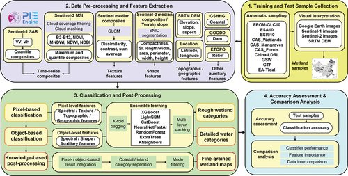
Figure 1 shows the overall framework for wetland classification and analysis. First, a wetland sample set for China was collected based on a sample collection strategy that combines automatic sampling and visual interpretation. Second, various features including spectral, texture, shape, topographic and geographic features were acquired and extracted from multi-source data including Sentinel-1/2 time series based on the Pixel Information Expert Engine (PIE-Engine) cloud platform. Third, a multi-stage wetland classification method integrating pixel-based and object-based strategies using the ensemble learning algorithm was developed, and fine-grained maps were derived for national wetland reserves. Lastly, accuracy assessment and comparison analysis were conducted to evaluate the reliability and effectiveness of the proposed method. Details on each step are provided in follows.

Figure 1. The framework for wetland classification and analysis.

2.1. Study area

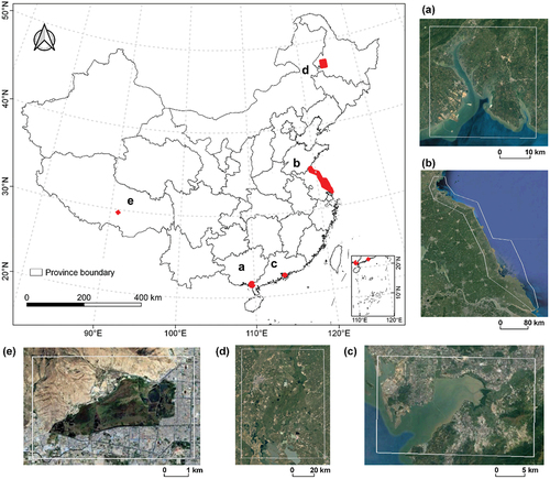
To construct a wetland sample set that encompasses diverse wetland categories, the entire country of China was taken as sampling area. Based on the sample set, experiments were conducted to demonstrate its potential to improve wetland classification accuracy. Subsequently, five national wetland reserves in China were selected to test the proposed method for mapping wetland categories. Specifically, the five reserves (Figure 2) include Guangxi Beilun Estuary National Nature Reserve (Site 1), Yancheng National Nature Reserve (Site 2), Mai Po Marshes and Inner Deep Bay (Site 3), Zhalong (Site 4) and Lalu National Nature Reserve (Site 5). Among them, Sites 1–4 have been included in the List of Ramsar Wetlands of International Importance. Specifically, Site 1 (109°27”−109°48’E, 21°25”-21°46’N) is a coastal wetland spanning an area of 1417 km² characterized by contiguous bay mangrove forest. Site 2 (119°4”−122°2’E, 31°39”-35°8’N) covers a vast area of 26,550 km² and has a representative tidal wetland ecosystem. Site 3 (113°51”−114°6’E, 22°24”-22°33’N) spans an area of 425 km² and comprises wetland areas such as artificial ponds and tidal flats. Site 4 situated in Heilongjiang Province (123°45”−124°46’E, 46°41”-47°35’N) covers an area of 7686 km² and holds an inland wetland ecosystem dominated by reed swamps. Site 5 (91°3”−91°7’E, 29°39”-29°41’N) is an alpine wetland covering an area of 28 km² situated on the Qinghai-Tibet Plateau.

Figure 2. Locations of five national wetland reserves in China. (a) Site 1 (Guangxi Beilun Estuary National Nature Reserve), (b) Site 2 (Yancheng National Nature Reserve), (c) Site 3 (Mai Po Marshes and Inner Deep Bay), (d) Site 4 (Zhalong), (e) Site 5 (Lalu National Nature Reserve). Google Earth imagery is shown in the background.

2.2. Classification system

According to the Ramsar Convention definition of wetlands (Gong et al. 2010) and considering the specific wetland characteristics in China and the suitability of remote sensing images, a wetland classification system was designed for this study (Table 1). Based on previous research in China (Niu et al. 2012), the classification system incorporates 14 fine-grained wetland categories. Additionally, for non-wetland areas, the classification system refers to the International Geosphere-Biosphere Project classification system (Loveland et al. 2000), and includes six categories. A detailed description of each category is listed in Table S1.

Table 1. The wetland classification system used in this study.

Category I	Category II	Category III
Wetland	Coastal wetland	Coastal swamp
		Coastal marsh
		Shallow marine water
		Estuarine water
		Lagoon
		Tidal flat
	Inland wetland	Inland swamp
		Inland marsh
		River
		Lake
		Floodplain
	Artificial wetland	Reservoir/pond
		Canal/channel
		Salt pan/aquaculture pond
Non-wetland	Cropland
	Forest
	Grassland
	Impervious
	Barren land
	Snow/ice

2.3. Data source

The detailed information of data utilized is summarized in Table 2 and Table S2.

Table 2. The detailed information of data utilized in this study.

Type	Data source	Spatial resolution	Time
Synthetic Aperture Radar (SAR)	Sentinel-1 ground range detected data (GRD)	10 m	2021
Multi-Spectral Imagery (MSI)	Sentinel-2 Level-2 surface reflectance data (SR)	10–20 m	2021
Google Earth images	Google Earth data	<1 m (highest)	2020–2021 (most)
Topography	Shuttle Radar Topography Mission Digital Elevation Model data (SRTM DEM)	30 m	2000
Land cover	Finer Resolution Observation and Monitoring of Global Land Cover (FROM-GLC10)	10 m	2017
	European Space Agency WorldCover dataset (ESA10)	10 m	2020
	Esri Land Cover dataset (ESRI10)	10 m	2020
Wetland maps	National Wetland Mapping Dataset of China (CAS_Wetlands)	30 m	2015
	Mangrove Mapping Dataset of China (CAS_Mangroves)	30 m	2015
	Coastal Aquaculture Pond Mapping Dataset of China (CAS_Ponds)	30 m	2015
	China’s Surface Water Bodies, Large Dams, Reservoirs and Lakes Dataset (China-LDRL)	30 m	2019
	Global Surface Water Mapping Dataset (GSW)	30 m	2021
	Global Tidal Flat Mapping Product (GTF)	30 m	2016
	Multi-class Tidal Wetland Dataset for East Asia (EA-Tidal)	10 m	2020
Other datasets	Global Self-consistent, Hierarchical, High-resolution Geography Database (GSHHG)	/	2017
	Global Georeferenced Database of Dams (GOODD)	/	2020
	Global Relief Model data (ETOPO)	15 arc-second	2022

2.3.1. Sentinel data

Sentinel-1 and Sentinel-2 imagery from the year 2021 were used as primary data sources for sample collection and wetland classification. All Sentinel data were acquired from the European Space Agency (ESA), and processed using the PIE-Engine cloud platform. PIE-Engine is an online remote sensing cloud computing platform that combines large-scale remote sensing data and computing resources to enable complex image processing, providing open data and elastic computing force support for research in the field of earth science (Chang et al. 2022).

Specifically, the Sentinel-1 data used in the study were ground range detected (GRD) data, which were processed based on the Sentinel-1 Toolbox. The Sentinel-1 GRD data consisted of vertical-vertical (VV) and vertical-horizontal (VH) polarization bands. On the other hand, the Sentinel-2 data used in the study were orthorectified atmospherically corrected surface reflectance (SR) data. The Sentinel-2 SR data were processed using the sen2cor tool, including 10-m bands for near-infrared (NIR), red, green and blue, as well as 20-m bands for shortwave infrared (SWIR) and red edge. To mask out clouds in the Sentinel-2 scenes, quality assessment bands were utilized. Scenes with a cloud cover of less than 30% were selected for further analysis. In total, 954 Sentinel-2 images and 635 Sentinel-1 images were collected and processed across five national wetland reserves in the study, The spatial distribution of the collected images is shown in Figure S1, while the detailed temporal distribution of the Sentinel images is shown in Figure S2.

2.3.2. Elevation data

Elevation data, as shown in Figure S1, was obtained from the Shuttle Radar Topography Mission Digital Elevation Model (SRTM DEM) (Farr et al. 2007). It was acquired from the National Aeronautics and Space Administration and was used to aid in sample interpretation and wetland classification. It provides 30-m resolution elevation information in the year 2000.

2.3.3. Google earth data

High-resolution imagery from Google Earth was utilized to assist in sample collection for the study. Google Earth provides a comprehensive and seamless mosaic of multi-source remote sensing imagery across various zoom levels and collection time, which is valuable for visual interpretation.

2.3.4. Land cover and wetland maps

Some high-spatial-resolution land cover and wetland datasets were utilized to assist in sampling. The three global 10-m land cover datasets used contained Finer Resolution Observation and Monitoring of Global Land Cover 10-m dataset (FROM-GLC10) (Gong et al. 2019), 10-m ESA WorldCover dataset (ESA10) (Zanaga et al. 2021) and 10-m Esri Land Cover map (ESRI10) (Karra et al. 2021). FROM-GLC10 and ESA10 offer global land cover datasets for the years 2017 and 2020, respectively, using machine learning methods. ESRI10 provides a global land cover product for the year 2020 utilizing deep learning techniques. The non-wetland extents were extracted from the three land cover datasets and used for subsequent sample generation (Table S2).

Wetland thematic products (Table S2) used included CAS_Wetlands (Mao et al. 2020), CAS_Mangroves (Jia et al. 2018), CAS_Ponds (Ren et al. 2019), Global Surface Water Mapping Dataset (GSW) (Pekel et al. 2016), China’s Surface Water Bodies, Large Dams, Reservoirs and Lakes Dataset (China-LDRL) (Wang et al. 2022), GTF (Murray et al. 2019), and Multi-class Tidal Wetland Dataset for East Asia (EA-Tidal) (Zhang et al. 2022). CAS_Wetlands is a 30-m wetland thematic map generated using hierarchical and object-based classification of Landsat imagery from 2015. CAS_Mangroves and CAS_Ponds are 30-m maps depicting the distribution of mangroves and coastal aquaculture ponds in China based on Landsat images from 2015 and object-based classification methods, respectively. GSW records the maximum extent of global surface water since 1985 using Landsat data. China-LDRL maps lakes, reservoirs, large dams and other surface water bodies in China utilizing Landsat and Google Earth imagery from 2019. GTF provides global distribution information on tidal flats with Landsat imagery from 2016. EA-Tidal depicts salt marshes, mangroves, and tidal flats in East Asia at a 10-m resolution for the year 2020. The wetland extents were extracted from the above wetland products and used for subsequent sample generation (Table S2).

2.3.4. Other auxiliary data

Several other datasets were used to assist in wetland classification in the study. The coastline information was extracted from Global Self-consistent, Hierarchical, High-resolution Geography Database (GSHHG) (Wessel and Smith 1996). GSHHG is a high-resolution shoreline dataset that merges data from three public domain datasets, developed by the University of Hawaiʻi and National Oceanic and Atmospheric Administration (NOAA). The dam information was derived from Global Georeferenced Database of Dams (GOODD) (Mulligan, van Soesbergen, and Sáenz 2020) provided by King’s College London. It was developed by digitizing visible dams using satellite imagery from Google Earth. In addition, Global Relief Model data (ETOPO) (NOAA 2022) was obtained from NOAA at a 15 arc-second resolution to provide geophysical characteristics of the Earth’s surface.

2.4. Sample collection

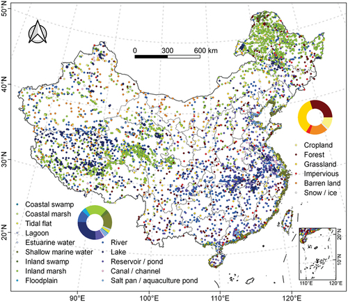
A sample collection strategy combining automatic sampling and visual interpretation was designed to improve efficiency. First, existing land cover and wetland maps were utilized to generate the sampling extent and sampling units. Then, the category of each sampling unit was visually interpreted and determined. Specifically, the wetland extent from seven wetland thematic products was merged, and 4000 potential wetland sampling units were derived and randomly distributed within this extent. Similarly, the non-wetland extent from three land cover products was intersected, and 2500 potential non-wetland sampling units were randomly generated within these areas. Additionally, another 500 sampling units were collected and randomly distributed outside the potential wetland and non-wetland extents. The obtained sampling units were visually interpreted with the assistance of Google Earth imagery, Sentinel time-series imagery, and SRTM DEM data. The size of each sampling unit was recorded, indicating the homogeneity of the area surrounding the sample point (Li et al. 2017). The sizes were classified into several levels, such as 1, 3 × 3, 9 × 9, 25 × 25, 51 × 51, and 99 × 99 pixels, considering the correspondence with the pixel sizes of common satellite data. Referring to the previous study (Zhao et al. 2014), the category of each sample was double-checked to ensure reliability, and uncertain or seriously mixed samples were removed. Finally, a total of 5070 samples with high confidence were collected, of which 3292 were identified as wetlands and 1778 were identified as non-wetlands. Figure 3 shows a detailed distribution of the national-scale sample set. In addition to the national-scale samples, additional samples were collected from five national wetland reserves for local validation. The specific number of samples collected at each site is provided: Site 1 (142 samples), Site 2 (143 samples), Site 3 (165 samples), Site 4 (160 samples), and Site 5 (57 samples).

Figure 3. Geographical distribution of the wetland sample set over China. The pie charts show the detailed distribution of wetland and non-wetland samples among categories.

2.5. Wetland classification

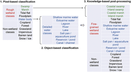
In this study, a multi-stage method was proposed for fine-grained wetland classification (Figure 4). First, a pixel-based ensemble learning algorithm was implemented to classify five rough wetland categories (swamp, marsh, tidal flat, floodplain, and water body) and six non-wetland categories (cropland, forest, grassland, impervious, barren land, and snow/ice). Second, an object-based ensemble learning approach was designed specifically to separate the water cover into more detailed eight categories (shallow marine water, estuarine water, lagoon, river, lake, salt pan/aquaculture pond, reservoir/pond, and canal/channel). Third, the results from the pixel-based and object-based classifications were integrated and refined using knowledge-based post-processing procedures to map 14 fine-grained wetland categories, including coastal swamp, coastal marsh, shallow marine water, estuarine water, lagoon, tidal flat, inland swamp, inland marsh, river, lake, floodplain, reservoir/pond, canal/channel, and salt pan/aquaculture pond.

Figure 4. The conception of the multi-stage wetland classification.

2.5.1. Feature extraction

For wetland classification in this study, both pixel-based and object-based features were extracted (as listed in Tables 3 and 4). Apart from Sentinel-2 SR, several commonly used spectral indexes were calculated, including the Normalized Difference Vegetation Index (NDVI), Normalized Difference Built-up Index (NDBI), Normalized Difference Water Index (NDWI), and Modified Normalized Difference Water Index (MNDWI). To account for seasonal variations among different wetland categories (Liu et al. 2020), quantile composites were computed for each band and index to provide simplified time-series information. To capture the maximum extent of water and vegetation (Jia et al. 2020), the maximum NDWI and NDVI values were used to obtain the wettest and greenest composites. In addition, quantile composites were computed for Sentinel-1 bands to supplement the information from Sentinel-2 and enhance the classification accuracies (Peng et al. 2023). Besides, texture features (dissimilarity, contrast, variation, and sum average) were calculated to add spatial relationship information of pixels. Specifically, texture features were derived using gray level co-occurrence matrix (GLCM) (Haralick, Shanmugam, and Dinstein 1973) based on Sentinel-1 (VH and VV) and Sentinel-2 (NDWI and NDVI) median composite images. The neighborhood size for GLCM was set to 3 and the directional bands were averaged.

Table 3. Pixel-based features adopted for wetland classification.

Type	Data source	Band/index	Feature
Time-series composites	Sentinel-2 time series	B2, B3, B4, B8, B5, B6, B7, B8A, B11, B12	Maximum and quantile (0,10,25,50,75,90 and 100) composites
		Normalized Difference Vegetation Index (NDVI) = (B8-B4)/(B8+B4)
		Normalized Difference Built-up Index (NDBI) = (B11-B8)/(B11+B8)
		Normalized Difference Water Index (NDWI) = (B3-B8)/(B3+B8)
		Modified Normalized Difference Water Index (MNDWI) = (B3-B11)/(B3+B11)
	Sentinel-1 time series	VV, VH	Quantile (0,10,25,50,75,90 and 100) composites
Texture features	Sentinel-2 median composites	NDVI, NDWI	Gray level co-occurrence matrix (GLCM) (dissimilarity, contrast, variation and sum average)
	Sentinel-1 median composites	VV, VH
Topographic features	Shuttle Radar Topography Mission Digital Elevation Model (SRTM DEM)	Elevation	Slope, aspect
Geographic features	Location	Latitude, longitude	Sine and cosine values

Table 4. Object-based features adopted for wetland classification.

Type	Data source	Feature	Description
Spectral features	Sentinel-2 median composites	B2, B3, B4, B8, B5, B6, B7, B8A, B11, B12, NDVI, NDBI, NDWI and MNDWI	Mean values of an object
Shape features	Simple Non-Iterative Clustering (SNIC) segmentation results	Compactness	Product of the length and width of an object divided by number of its pixels
		Shape index	Perimeter of an object divided by four times the square root of area
		Length/width	Ratio of length to width of an object
		Area	Area of an object
		Perimeter	Perimeter of an object
		Width	Width of an object
		Height	Height of an object
Auxiliary features	Global Self-consistent, Hierarchical, High-resolution Geography Database (GSHHG)	Coastal	Proportion of coastal area of an object
	Global Georeferenced Database of Dams (GOODD)	Dam	Intersection with the 400-m buffer of dams of an object
	Global Relief Model (ETOPO)	Relief	Mean bedrock elevation of an object

To enhance water classification, object-based shape features were computed. First, the Simple Non-Iterative Clustering (SNIC) method (Achanta and Süsstrunk 2017) was applied to obtain superpixel segmentation results based on Sentinel-2 median composites and terrain slope derived from SRTM DEM data. Further, to capture the geometric characteristics of different water categories (Mao et al. 2020), shape features including compactness, shape index, length/width, area, perimeter, width, and height were calculated for each object. Simultaneously, mean values of SR and indexes were extracted from Sentinel-2 median composites for each object.

To assist in wetland classification, additional auxiliary features including topographic features (elevation, slope, and aspect) derived from SRTM DEM data and geographic features (longitude and latitude) were utilized. In addition, at the object level, the proportion of coastal area (Coastal) was derived based on GSHHG data to separate coastal and inland categories, and the intersection with the 400-m buffer of the dams (Dam) based on GOODD data was calculated to provide information related to reservoirs, and bedrock elevation information (Relief) based on ETOPO data was extracted for helping identify shallow marine water.

2.5.2. Pixel-based classification

In this study, an ensemble learning algorithm was developed for the first stage based on pixel-based features (Table 3) to classify 11 rough categories, including five rough wetland categories (swamp, marsh, tidal flat, floodplain, and water body) and six non-wetland categories (cropland, forest, grassland, impervious, barren land, and snow/ice).

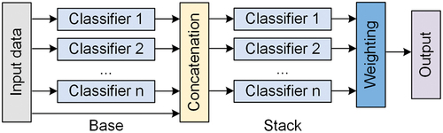
Ensemble learning often outperforms individual classifiers by combining predictions of multiple classifiers. Here, ensemble learning classifiers were trained utilizing a multi-layer stacking strategy. The architecture is depicted in Figure 5. Each stack layer consisted of multiple individual base classifiers. The output predictions of the base classifiers were concatenated with the original input features and fed into multiple stacker classifiers at higher layers. The stacker classifiers of the previous layer could be further regarded as base classifiers of the next layer. The final stack layer applies ensemble selection to aggregate predictions of stacker classifiers in a weighted manner (Caruana et al. 2004). Meanwhile, a k-fold bagging strategy was adopted at all stack layers to mitigate overfitting issues and further enhance performance.

Figure 5. The architecture of ensemble learning with multi-layer stacking strategy, shown here with n types of base classifiers and 2 stack layers.

Automatic ensemble learning was implemented by utilizing the AutoGluon framework (Erickson et al. 2020). It helped train classifiers and conduct procedures including model selection, model ensembling, and hyperparameter tuning automatically. Types of base classifiers used here contained XGBoost, CatBoost, k-nearest neighbors, neural networks, extremely randomized trees, random forests, and Light Gradient Boosting Machine (LightGBM). The parameters of classifiers were initialized using default values and optimized automatically. Specifically, for XGBoost, the learning rate and number of iterations were set to 0.1 and 10,000, respectively. In CatBoost, the learning rate and number of iterations were set to 0.05 and 10,000, respectively. For k-nearest neighbors, weight functions included distance and uniform. For neural networks, batch size, and epoch were 256 and 30, respectively, and target and base learning rates were set to 0.1 and 0.01, respectively. In extremely randomized trees and random forests, the number of trees was 300, and the criteria used included Gini and entropy. In LightGBM, classifiers were trained with three groups of parameter settings, including one with default parameters, one enabling the use of extremely randomized trees, and one with custom parameters enabling larger models. Basically, in LightGBM, the number of iterations, learning rate, number of leaves, fraction of features, and minimal number of data in one leaf were 10,000, 0.05, 31, 1, and 20, respectively, boosting type used was traditional Gradient Boosting Decision Tree. For the large LightGBM model, the learning rate, number of leaves, fraction of features, and minimal number of data in one leaf were set to 0.03, 128, 0.9, and 3, respectively. The overall number of stack layers was three and the number of bagging folds was five. All parameter settings of classifiers are listed in Table S3.

2.5.3. Object-based classification

In the second-stage object-based classification, the water cover was separated into eight detailed categories including shallow marine water, estuarine water, lagoon, river, lake, salt pan/aquaculture pond, reservoir/pond, and canal/channel.

The Sentinel-2 median composites and terrain slope images were first segmented using the SNIC algorithm. SNIC can group neighboring pixels into clusters effectively in a bottom-up, seed-based manner (Tu et al. 2020). After multiple experiments and visual comparisons in the study area, SNIC parameter settings were used as follows. Superpixel seed location spacing was set to 16 pixels, and connectivity and compactness were set to 8 and 0.5, respectively.

Based on the segmentation results, discriminative object-based spectral, shape, and auxiliary features, as listed in Table 4, were calculated to facilitate water classification. Referring to previous studies (Mao et al. 2020; Peng et al. 2023), shape features, such as compactness, shape index, and length/width, help separate water cover since various water categories show geometric differences. Auxiliary features, including Coastal, Dam, and Relief, can aid in the identification of specific water categories such as reservoirs, shallow marine water, and lagoons.

To achieve detailed water classification, an ensemble learning model was further trained to automatically construct the classification rules with the object-based features in this study. The parameters of classifiers used in this stage were the same as those described in the pixel-based stage, though the number of stack layers was reduced to two.

2.5.4. Post-processing

The results of the pixel-based and object-based classifications were merged to preserve both detailed information from pixel-based classification and precise information from object-based classification. Specifically, the areas classified as water in the pixel-based classification results were relabeled using the detailed water categories from the object-based classification results.

Besides, swamps and marshes identified in the pixel-based classification results were separated into coastal and inland categories based on coastal region vectors derived from GSHHG data (Mao et al. 2020). Then, to reduce noise, mode filtering with a 3 × 3 kernel was leveraged to further post-process classification results. Finally, the classification results refined with the knowledge-based post-processing procedures with 14 wetland categories were obtained.

2.6. Accuracy assessment and comparison analysis

The collected sample set was randomly separated into two parts, including training samples (70%) and test samples (30%). With confusion matrices, accuracy indicators, including F1 score, weighted F1 score, user’s accuracy, producer’s accuracy, kappa coefficient, and overall accuracy (Congalton, Oderwald, and Mead 1983; Story and Congalton 1986), were calculated. According to accuracies, training time, and prediction time, the trained pixel-based and object-based classifiers were evaluated.

Based on the mean decrease in accuracies, the relative importance of each feature to classifiers was quantified. Given that multi-source data and multi-dimensional features have been included in wetland classification, it would be helpful to explore the contribution of various types of data and features. Consequently, classification accuracies when using different groups of features were compared. For pixel-based classification, the compared feature groups included (a) Sentinel-1 features without texture (S1-notexture); (b) Sentinel-1 features (S1); (c) Sentinel-2 features without texture (S2-notexture); (d) Sentinel-2 features (S2); (e) topographic and geographic features (Others); (f) S1 and S2 features (S1+S2); (g) S1 features and others (S1+Others); (h) S2 features and others (S2+Others); (i) S1, S2 features without texture and others (S1-notexture+S2-notexture+Others); (j) S1, S2 features and others (S1+S2+Others). For object-based classification, the compared feature combinations included (a) spectral features (Spectral); (b) shape features (Shape); (c) auxiliary features (Others); (d) spectral and shape features (Spectral+Shape); (e) spectral and auxiliary features (Spectral+Others); (f) shape and auxiliary features (Shape+Others); (g) spectral, shape and auxiliary features (Spectral+Shape+Others).

To reflect the reliability of the proposed wetland classification method, the derived wetland maps in five national reserves were intercompared with other existing products, including 30-m wetland mapping product CAS_Wetlands in 2015 and 10-m land cover mapping dataset FROM-GLC10 in 2017. To facilitate the comparison, wetland and water body categories were extracted from FROM-GLC10, and remapped into wetland maps.

Besides, to further prove the effectiveness, the proposed multi-stage ensemble learning method was compared with a single-stage ensemble learning method based on the overall accuracy and F1 score per class. Specifically, the single-stage ensemble learning classifier was trained with input pixel-based features and directly used to predict fine-grained categories. The performance of the wetland classification method was also validated across regions. Apart from classifiers trained with the total samples (global classifiers), classifiers based on local samples (local classifiers) were also trained. Specifically, five local classifiers were trained using samples centered on each national wetland reserve and its 1.5° buffer ring. The accuracies of global and local classifiers were tested across five national wetland reserves.

To investigate the reliability and potential of the proposed wetland mapping method, its robustness was tested under sample simulation scenarios. Referring to the theory of “stable classification with limited sample” (Gong et al. 2019), the wetland sample set was used to explore the sensitivity and tolerance of the pixel-based ensemble learning classifier to sample size and errors. Two groups of experiments were implemented. First, the number of training samples was progressively reduced by 1% each time. Second, class labels in part of the total samples were randomly altered, and such noisy samples with wrong labels were used to train classifiers. The variation of the mean overall accuracy was recorded. The results could provide insights into the migration potential of the sample set and the proposed method for mapping over time-series data since labels of samples would be changed as land cover changes.

3. Results

3.1. Performance of different classifiers

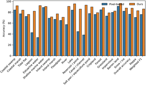
The comparisons of classifiers in Tables 5 and 6 demonstrated that the ensemble learning algorithm effectively improved the accuracies of both pixel-based (first-stage) and object-based (second-stage) wetland classification. The ensemble learning classifiers yielded higher accuracies than base classifiers including CatBoost, random forest, and XGBoost. Specifically, pixel-based and object-based overall accuracies of the ensemble learning classifiers were 20.84% and 11.07% higher than those of the k-nearest neighbors classifiers. Additionally, high-stack-layer classifiers tended to outperform low-stack-layer classifiers. When the ensemble learning classifier was increased from the second to the third stack layer, pixel-based overall accuracy was improved from 88.23% to 89.08%. In terms of running time, neural networks and large LighGBM classifiers performed poorly since they took a relatively longer time for training and prediction. In general, ensemble learning classifiers with the multi-layer stacking strategy showed the best performance regarding accuracies for both first-stage rough wetland categories (overall accuracy: 89.08%, kappa: 84.89%) and second-stage detailed water categories (overall accuracy: 95.10%, kappa: 85.32%).

Table 5. Comparison results of different classifiers according to first-stage pixel-based classification accuracy and running time×.

Classifier	Stack layer	Overall accuracy	Weighted F1	Kappa	Training time (s)	Prediction time (s)
Ensemble_L3	3	89.08%	88.12%	84.89%	1.3951	0.0015
Ensemble_L2	2	88.23%	87.62%	83.41%	1.5053	0.0013
CatBoost_L2	2	87.89%	87.13%	83.27%	121.8304	0.1119
RandomForestEntr_L2	2	87.81%	87.08%	83.26%	3.6804	0.7267
NeuralNet_L2	2	87.68%	86.93%	83.16%	177.6707	1.3805
XGBoost_L2	2	87.67%	86.90%	83.11%	313.5393	0.1746
RandomForestGini_L2	2	87.55%	86.88%	83.09%	2.6438	0.7317
LightGBMXT_L2	2	87.43%	86.70%	82.96%	105.1335	0.1400
LightGBMLarge_L1	1	87.39%	86.42%	82.96%	670.6065	1.1883
LightGBM_L2	2	87.32%	86.29%	82.91%	193.5103	0.1149
LightGBM_L1	1	87.17%	86.22%	82.86%	134.4801	0.4969
ExtraTreesGini_L2	2	87.14%	86.07%	82.77%	0.9878	0.7208
LightGBMLarge_L2	2	87.56%	85.96%	82.63%	312.8892	0.2953
ExtraTreesEntr_L2	2	87.04%	85.74%	82.61%	0.9119	0.7349
XGBoost_L1	1	86.97%	85.69%	82.35%	415.7402	0.3938
NeuralNet_L1	1	86.84%	85.66%	82.31%	469.5535	2.4058
CatBoost_L1	1	86.65%	85.57%	82.27%	318.3589	0.1687
LightGBMXT_L1	1	86.63%	84.96%	82.24%	162.6078	0.7994
RandomForestEntr_L1	1	86.32%	84.80%	82.21%	2.4335	0.5753
RandomForestGini_L1	1	86.03%	84.47%	81.93%	2.0811	0.5598
ExtraTreesEntr_L1	1	85.68%	84.04%	80.87%	0.9052	0.5982
ExtraTreesGini_L1	1	85.65%	83.94%	80.79%	1.0127	0.6255
KNeighborsDist_L1	1	69.72%	68.39%	62.85%	0.0651	3.7477
KNeighborsUnif_L1	1	68.24%	67.43%	60.02%	0.0630	3.8482

*Note: Explanations of classifier abbreviations can be found in Table S3. The suffix in classifier names, such as L3, L2, and L1, denotes stack layer.

Table 6. Comparison results of different classifiers according to second-stage object-based classification accuracy and running time×.

Classifier	Stack layer	Overall accuracy	Weighted F1	Kappa	Training time (s)	Prediction time (s)
Ensemble_L2	2	93.10%	91.18%	85.32%	0.2016	0.0023
RandomForestEntr_L1	1	92.34%	89.53%	84.73%	0.4286	0.0519
RandomForestGini_L1	1	92.40%	89.60%	81.92%	0.4415	0.0474
NeuralNet_L1	1	91.92%	88.84%	81.80%	418.4889	4.3730
XGBoost_L1	1	90.73%	88.45%	78.22%	37.1230	3.4959
ExtraTreesEntr_L1	1	89.33%	87.40%	77.12%	0.4265	0.0466
LightGBMLarge_L1	1	88.61%	87.05%	73.70%	187.7901	0.8240
ExtraTreesGini_L1	1	88.20%	86.18%	71.30%	0.4208	0.0470
LightGBM_L1	1	87.65%	85.82%	70.60%	48.8723	0.7386
LightGBMXT_L1	1	86.96%	84.81%	69.62%	45.6386	0.8445
CatBoost_L1	1	85.27%	82.02%	66.53%	41.6439	0.2258
KNeighborsDist_L1	1	83.73%	81.54%	65.16%	0.0059	0.0162
KNeighborsUnif_L1	1	82.03%	79.85%	63.20%	0.0123	0.0160

*Note: Explanations of classifier abbreviations can be found in Table S3. The suffix in classifier names, such as L3, L2, and L1, denotes stack layer.

The evaluated overall wetland classification accuracies using the proposed multi-stage method are presented in Table 7. Results implied that classification accuracy was relatively high. The overall accuracy, kappa, and weighted F1 reached 87.39%, 82.80%, and 86.02%, respectively. These results indicated the effectiveness of the proposed method for wetland classification. Among the non-wetland categories, forest, barren land, and snow/ice yielded high accuracies, with F1 scores of 88.45%, 96.31%, and 87.72%, respectively. In terms of coastal wetland categories, shallow marine water, estuarine water, and coastal swamp were well separated, with both user’s and producer’s accuracies exceeding 85%. Tidal flat had a high user’s accuracy of 92.22%, and a moderate producer’s accuracy of 64.83%, which indicated some omission errors. These errors might be related to the disturbance of tidal rise and fall. As for inland wetland categories, water categories, such as river and lake, achieved relatively high accuracies, with F1 values of more than 90%. However, the identification of floodplains was challenging, with a relatively low F1 value of 70.80%, which might result from confusion with barren land. Regarding artificial wetlands, the accuracies of three categories including salt pan/aquaculture pond, canal/channel, and reservoir/pond were satisfying, with F1 scores over 85%.

Table 7. Overall wetland classification accuracy of the proposed multi-stage method.

Class	User’s accuracy	Producer’s accuracy
Coastal swamp	95.24%	88.71%
Coastal marsh	90.30%	78.28%
Shallow marine water	86.53%	94.94%
Estuarine water	94.89%	89.73%
Lagoon	79.54%	84.63%
Tidal flat	92.22%	64.83%
Inland swamp	67.14%	76.32%
Inland marsh	74.04%	80.33%
River	89.26%	92.51%
Lake	93.93%	96.93%
Floodplain	64.95%	77.80%
Reservoir/pond	83.64%	88.06%
Canal/channel	91.79%	94.41%
Salt pan/aquaculture pond	90.83%	88.57%
Cropland	73.40%	85.98%
Forest	86.55%	90.44%
Grassland	80.84%	76.90%
Impervious	76.65%	88.52%
Barren land	95.30%	97.35%
Snow/ice	91.89%	83.91%
Overall accuracy	87.39%
Kappa	82.80%
Weighted F1	86.02%

3.2. Relative contribution of features

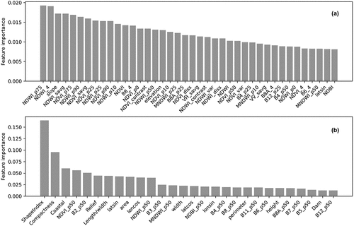
According to the relative importance, the top critical features for pixel-based and object-based wetland classification are illustrated in Figure 6. For pixel-based rough wetland classification, spectral indexes (NDVI and NDWI), texture features (sum average and contrast), and topographic features (slope and elevation) were identified as important leading predictors. It makes sense that the quantile and maximum composites of the spectral indexes help distinguish wetlands since they can provide dynamic information over time. Apart from spectral indexes, the relative importance of NIR (B8) and red edge (B8A) SR was high, which might be related to the apparent difference between vegetation and wetlands in these spectral ranges. The high importance of texture features was also reasonable considering the texture differences of categories such as swamps and marshes. Simultaneously, the significant contribution made by the topographic features indicated that the topographic environment was a critical factor influencing the distribution of wetlands. For object-based wetland classification, shape features (such as shape index and compactness) were found to be crucial and helped the separation of detailed water categories most. For example, shape features could contribute to the classification of patchy and linear water objects. Moreover, auxiliary features (such as coastal, relief, and geographic location) were also essential for object-based classification, since such information could be useful for distinguishing some categories with special distribution characteristics, such as shallow marine water and lagoon.

Figure 6. The relative importance of features for (a) pixel-based classification and (b) object-based classification. Note: explanations of feature names can be found in Tables 3 and 4. Suffixes in the feature names such as p50 and p75 denote quantile values. Suffixes including diss, contrast, var, and savg, refer to dissimilarity, contrast, variation, and sum average features. The suffix ‘_4’ stands for the wettest composites. Features including latsin, latcos, lonsin, and loncos represent sine and cosine values of latitude and longitude.

Different classification accuracies were achieved using different combinations of features (Tables 8 and 9). For first-stage pixel-based classification, the accuracies from Sentinel-2 features (overall accuracy: 84.08%, kappa: 79.01%) were much higher than those from Sentinel-1 features (overall accuracy: 71.29%, kappa: 62.57%) or other features (topographic and geographic features) (overall accuracy: 69.15%, kappa: 60.43%). Introducing texture features helped improve classification accuracies. For example, compared to classification with Sentinel-2 spectral features alone, overall accuracy and kappa of pixel-based classification including Sentinel-2 texture features were improved by 1.80% and 0.57%, respectively. In addition, integrating features from different sources could yield relatively good accuracies. For instance, for rough wetland categories, the combination of Sentinel-2 and Sentinel-1 features yielded an overall accuracy of 86.69%, while the combination of Sentinel-2 and other features yielded an overall accuracy of 86.91%. Moreover, integrating features from all three sources (Sentinel-1, Sentinel-2, and other features) achieved the best accuracy for pixel-based classification, resulting in an overall accuracy of over 89%. For second-stage object-based classification, the use of shape features yielded higher accuracies (overall accuracy: 82.76%, kappa: 71.13%) compared with spectral features (overall accuracy: 72.59%, kappa: 60.06%) or other auxiliary features (overall accuracy: 74.31%, kappa: 60.96%). The combination of spectral, shape, and other auxiliary features yielded the best performance according to overall accuracy and F1 scores for most categories. In summary, the integration of high-resolution spectral, texture, shape, and topographic features from multi-source remote sensing data, along with geographic and auxiliary features, provided a multi-dimensional perspective for revealing the distribution and patterns of fine-grained wetland categories.

Table 8. Comparison of pixel-based classification accuracy with different combinations of features×.

Class	S1 -notexture	S1	S2 -notexture	S2	Others	S1 +S2	S1 +Others	S2 +Others	S1-notexture +S2-notexture +Others	S1 +S2 +Others
Swamp	54.66%	55.55%	64.69%	73.29%	71.95%	68.55%	74.32%	75.89%	74.77%	74.84%
Marsh	59.22%	59.21%	68.69%	68.63%	67.30%	70.06%	72.31%	74.96%	74.73%	77.25%
Tidal flat	57.21%	60.76%	70.56%	74.95%	61.07%	72.43%	63.68%	75.11%	74.30%	76.14%
Floodplain	52.32%	58.29%	64.71%	70.00%	53.14%	69.49%	58.56%	67.40%	69.48%	70.80%
Water body	76.97%	81.98%	92.36%	93.20%	77.68%	94.22%	88.55%	92.62%	92.94%	95.03%
Cropland	51.68%	56.50%	74.97%	77.96%	36.88%	76.73%	69.47%	78.20%	76.92%	79.19%
Forest	68.27%	72.49%	83.78%	84.40%	77.93%	85.56%	83.20%	86.73%	86.73%	88.45%
Grassland	42.54%	44.06%	67.63%	73.26%	62.56%	71.52%	67.32%	75.82%	77.62%	78.82%
Impervious	52.38%	65.16%	58.56%	69.63%	15.43%	78.80%	71.86%	73.80%	76.41%	82.16%
Barren land	64.60%	69.79%	91.23%	93.04%	75.28%	93.74%	84.03%	94.13%	94.96%	96.31%
Snow/ice	54.85%	41.07%	87.39%	88.35%	66.56%	87.28%	64.05%	86.46%	88.09%	87.72%
Overall accuracy	66.23%	71.29%	82.28%	84.08%	69.15%	86.69%	82.41%	86.91%	87.87%	89.08%
Kappa	56.93%	62.57%	78.44%	79.01%	60.43%	82.17%	75.75%	81.83%	81.29%	84.89%
Weighted F1	64.72%	70.42%	81.74%	83.56%	68.76%	85.97%	81.71%	86.26%	87.01%	88.12%

*Note: Lines 2 to 12 are the F1 score per class.

Table 9. Comparison of object-based classification accuracy with different combinations of features×.

Class	Spectral	Shape	Others	Spectral +Shape	Spectral +Others	Shape +Others	Spectral +Shape +Others
Lagoon	58.05%	77.79%	71.85%	80.06%	73.06%	81.30%	82.59%
Estuarine water	77.67%	76.24%	89.91%	84.67%	90.67%	91.82%	92.67%
Shallow marine water	78.54%	83.41%	87.05%	85.44%	87.94%	89.32%	90.50%
River	74.56%	83.56%	64.99%	85.78%	79.00%	89.21%	90.64%
Lake	70.87%	90.61%	74.67%	92.88%	75.88%	94.12%	95.41%
Reservoir/pond	41.48%	55.86%	84.34%	57.10%	85.22%	86.95%	86.18%
Canal/channel	78.14%	86.56%	68.43%	88.77%	82.44%	92.25%	93.33%
Salt pan/aquaculture pond	59.72%	85.56%	67.56%	87.11%	70.90%	88.13%	89.78%
Overall accuracy	72.59%	82.76%	74.31%	87.93%	76.21%	91.38%	93.10%
Kappa	60.06%	71.13%	60.96%	75.32%	63.78%	81.23%	85.32%
Weighted F1	71.48%	78.41%	72.11%	86.44%	75.09%	88.83%	91.18%

*Note: Lines 2 to 9 are the F1 score per class.

3.3. Wetland maps for five national wetland reserves

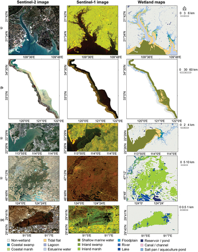
The 10-m wetland maps were derived for five national wetland reserves using the proposed classification method. As shown in Figure 7, the results could accurately depict the distribution and composition of wetlands in each reserve. In Site 1, Site 2, and Site 3, the primary wetland categories were coastal wetlands, including tidal flats, shallow marine water, coastal marshes and artificial wetlands like salt pans/aquaculture ponds. Additionally, Site 1 and Site 3 also exhibited a dense distribution of coastal swamps. In contrast, the majority of wetlands in Site 4 and Site 5 belonged to inland categories such as inland marshes, lakes, and rivers.

Figure 7. The wetland mapping results of five national wetland reserves in 2021. (a) Site 1, (b) Site 2, (c) Site 3, (d) Site 4, (e) Site 5. Figures in the first and second columns are Sentinel-2 and Sentinel-1 composite images in 2021, respectively.

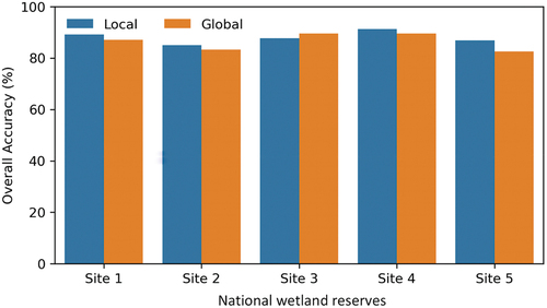
Quantitative comparisons of the performance of global and local classifiers across the five national wetland reserves are presented in Figure 8. Except for Site 3, the overall accuracies of the local classifiers were higher than those of the global classifiers. The largest and smallest differences in overall accuracies between local and global classifiers were observed for Site 5 (4.34%) and Site 4 (1.79%), respectively. Though local classifiers outperformed global classifiers slightly, global classifiers illustrated plausible accuracies across the five national wetland reserves with a mean overall accuracy of 86.40%. In general, these results proved the reliability of employing the proposed method in accurately mapping wetland categories in different regions.

Figure 8. Comparison of global and local classifiers across five national wetland reserves using overall accuracy.

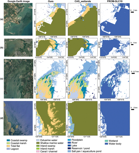
Intercomparison results with other products further demonstrated the quality of the derived wetland maps and the superiority of the proposed method. The visualization results in selected locations are shown in Figure 9. Compared to FROM-GLC10, CAS_wetlands, and our mapping results could identify multi-category wetland distribution. Simultaneously, our mapping results exhibited a more reasonable and detailed representation of wetland patterns. For instance, our mapping results depicted fine-grained and precise patterns of salt pans/aquaculture ponds, while CAS_wetlands slightly overestimated the wetland areas. Besides, our mapping results had relatively high characterization capabilities in wetlands such as tidal flats. Overall, though data sources and classification methods vary among products, our derived wetland maps provided the best visual correspondence with Google Earth images.

Figure 9. Comparison of our wetland mapping results, CAS_wetlands, and FROM-GLC10 in selected locations. (a) centered at 109.5°E, 21.5°N; (b) centered at 114.0°E, 22.5°N; (c) centered at 109.7°E, 21.6°N; (d) centered at 121.0°E, 33.0°N. Figures in the first column are Google Earth images.

4. Discussion

4.1. Effectiveness of the proposed wetland classification method

A fine-grained wetland mapping method that integrates pixel-based and object-based classification using multi-dimensional features and the ensemble learning algorithm was developed in this study.

Object-based classification can help construct strong features and information and thereby contribute to improving wetland mapping accuracy (Amani et al. 2022). However, it may cause a loss of spatial details. To address this, in this study, pixel-based and object-based classification methods were combined to achieve better wetland mapping results, considering a balance of accuracies and spatial details. As illustrated in Figure 9, the derived wetland maps in five national wetland reserves preserved more details compared to CAS_wetlands which relied solely on an object-based method (Mao et al. 2020). This highlights the advantage of integrating pixel-based classification as a basis for maintaining spatial details in wetland maps. Simultaneously, as shown in Figure 10, compared with the results obtained directly from a single-stage pixel-based ensemble learning method, the proposed multi-stage method yielded better performance. This indicates the effectiveness of merging and leveraging object-based features and classification results.

Figure 10. Comparison in classification accuracy of single-stage pixel-based method and our proposed multi-stage method. Class-level accuracies are F1 scores.

In recent studies, machine learning algorithms have outperformed traditional methods (Wei et al. 2022). In this study, the ensemble learning algorithm was used to integrate multiple machine learning algorithms and automatically construct efficient classifiers for wetland classification. Performance comparisons on various classifiers and features might provide insights for wetland mapping practice. Results showed that ensemble learning yielded the best wetland classification accuracies, compared with base classifiers such as XGBoost and random forest, despite needing longer running time. With the investigation of feature contribution, the results suggested that integrating multi-source data could provide important input features for wetland classification. In general, the quantitative and visualization results demonstrated the effectiveness of the ensemble learning algorithm. In this study, traditional machine learning algorithm was applied, although deep learning algorithms achieved better performance in some recent studies (Jamali and Mahdianpari 2022). The ensemble learning algorithm illustrated its potential and robustness in wetland classification with plausible accuracies. Besides, compared to deep learning algorithms, the ensemble learning algorithm could provide better interpretability according to feature importance.

4.2. Application potential of the sample set for large-scale mapping

A wetland sample set was presented under a classification system with 20 fine-grained categories in China in this study. Each sample was visually interpreted and double-checked using Sentinel imagery and Google Earth imagery, ensuring high reliability. Classification results based on the proposed method showed that the sample set performed well in terms of accuracy. Mapping results in the five national wetland reserves indicated that the sample set could support fine-grained mapping of wetland categories. This sample set is promising to form a base for future use in large-scale 10-m wetland mapping.

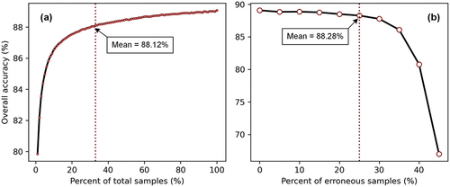
Simultaneously, the robustness of the sample set was also examined. As presented in Figure 11, the results implied that when the sample size was considerably smaller or a quarter of samples were in error, stable classification could still be achieved using the proposed method. Referring to stable classification (Gong et al. 2019), if the overall accuracy of the classifier trained using part of the samples is within 1% lower than that of the classifier trained using total samples, the classification is considered stable. From Figure 11a, the mean overall accuracy for pixel-based classification was relatively stable before using only 33% of the training samples (88.12% vs. 89.08%). So, only about 33% of the total samples need to be used to maintain a stable wetland classification (the overall accuracy gap was 0.96%). Furthermore, from Figure 11b, when the percentage of the erroneous training samples reached 25%, the mean overall accuracy for pixel-based wetland classification was within 1% from that obtained with unaltered samples. Therefore, the sample tolerance to errors is up to 25%. These results highlighted that by leveraging the ensemble learning algorithm, it was possible to use 33% of samples or samples containing 25% errors to achieve stable wetland classification results. Overall, this revealed the sensitivity and tolerance of the adopted ensemble learning classifier to sample size and errors. These results might guide wetland sample migration and application for long-time-series mapping in future research (Fekri et al. 2021).

Figure 11. Sample robustness to size reduction and errors based on pixel-based ensemble learning classifier. Variation of the mean overall accuracy with the (a) sample size and (b) impurity percentage of samples.

4.3. Advantage of the PIE-Engine cloud computing platform

With the advent of the era of remote sensing big data, various cloud computing platforms were developed to support rapid processing and analysis of massive data (Gorelick et al. 2017). The PIE-Engine platform used in this study is one of the important representatives. PIE-Engine is a spatiotemporal remote sensing cloud computing platform that integrates data, computing power, and algorithms by adopting container cloud technology. It can implement on-demand acquisition of remote sensing data and rapid processing of massive data. In this study, the PIE-Engine platform effectively supported the data processing and analysis tasks. Comparisons with Google Earth Engine (GEE) showed that the running of PIE-Engine was slightly longer than that of GEE owing to computing resource limitations, yet output results were mostly consistent. In general, the PIE-Engine platform used in this study is promising to provide more support for remote sensing and geospatial studies.

4.4. Limitations and future work

Some difficulties and limitations in this study should be addressed and improved in the future. Firstly, the same parameters were leveraged in the segmentation algorithm for all five national wetland reserves. While sensitivity analysis results showed that the chosen parameter settings (for example, compactness was set to 0.5) achieved the best mean classification accuracy in the study area (as shown in Figure S3), more flexible parameter setting methods should be explored to adapt to conditions in different regions in future research (Mui, He, and Weng 2015). Secondly, the adopted classification method yielded high-accuracy wetland maps, yet accuracies for some wetland categories such as floodplain, swamp, and marsh were relatively low. To overcome the challenge, the wetland classification method needs to be further enhanced in the future, probably by combining more effective auxiliary domain knowledge (Wang et al. 2020). Thirdly, the obtained wetland maps based on single-year images were insufficient to provide dynamic information. To monitor wetland changes and responses to environmental stressors, annual or seasonal wetland maps should be further produced in future works (Wu et al. 2022).

5. Conclusions

In this study, a novel multi-stage wetland classification method that integrates pixel-based and object-based strategies using the ensemble learning algorithm and multi-source remote sensing data was developed. A wetland sample set with 20 categories across China was constructed based on an efficient sample collection strategy that combines automatic sampling and visual interpretation. Comparison results suggested the ensemble learning algorithm achieved better performance than classifiers such as CatBoost, XGBoost, k-nearest neighbors, neural networks, extremely randomized trees, random forests, and LightGBM. The overall accuracy of the first-stage pixel-based classification using the ensemble learning algorithm reached 89.08%, while the second-stage object-based classification achieved an overall accuracy of 93.10%. In general, the proposed wetland classification method yielded high accuracies with overall accuracies, kappa, and weighted F1 scores of 87.39%, 82.80%, and 86.02%, respectively. Combining high-resolution spectral, radar, texture, shape, topographic and geographic features from multi-source data provided a multi-dimensional perspective for revealing the distribution of wetland categories. In addition to geographic and topographic information, time-series composites of spectral indexes (NDVI and NDWI), near-infrared (B8), and red-edge (B8A) SR, as well as texture features (sum average and contrast) were essential in pixel-based wetland classification, while shape features (shape index and compactness) were crucial for object-based water classification. Results for five national wetland reserves further illustrated the effectiveness of the proposed wetland classification method. Compared to other products such as CAS_Wetlands and FROM-GLC10, the wetland mapping results obtained using the proposed method could reflect a more detailed and fine-grained distribution of wetland categories. Overall, the results of this study proved the reliability and potential of the developed wetland classification method and the collected sample set on larger scales. The obtained wetland maps can provide support for wetland protection, evaluation, and management efforts.

Acknowledgments

We are grateful to ESA and Google for providing the satellite data.

Disclosure statement

The authors declare that they have no known competing financial interests or personal relationships that could have appeared to influence the work reported in this paper.

Data availability statement

The data that support the findings of this study are available upon request by contact with corresponding authors.

Supplementary material

Supplemental data for this article can be accessed online at https://doi.org/10.1080/15481603.2023.2286746

Additional information

Funding

The work was supported by the National Natural Science Foundation of China [42301461]; Open Research Fund Program of Key Laboratory of Digital Mapping and Land Information Application, Ministry of Natural Resources [ZRZYBWD202210].

References

- Achanta, R., and S. Süsstrunk. 2017. “Superpixels and Polygons Using Simple Non-Iterative Clustering.” Paper presented at the 2017 IEEE Conference on Computer Vision and Pattern Recognition (CVPR), Honolulu, HI, USA, 21-26 July 2017.
- Amani, M., M. Kakooei, A. Ghorbanian, R. Warren, S. Mahdavi, B. Brisco, A. Moghimi, et al. 2022. “Forty Years of Wetland Status and Trends Analyses in the Great Lakes Using Landsat Archive Imagery and Google Earth Engine.” Remote Sensing 14 (15): 3778. https://doi.org/10.3390/rs14153778.
- Assessment, M. E. 2005. Ecosystems and Human Well-Being: Wetlands and Water. Washington: World Resources Institute.
- Cai, Y., X. Li, M. Zhang, and H. Lin. 2020. “Mapping Wetland Using the Object-Based Stacked Generalization Method Based on Multi-Temporal Optical and SAR Data.” International Journal of Applied Earth Observation and Geoinformation 92:102164. https://doi.org/10.1016/j.jag.2020.102164.
- Caruana, R., A. Niculescu-Mizil, G. Crew, and A. Ksikes. 2004. “Ensemble Selection from Libraries of Models.” In Proceedings of the twenty-first international conference on Machine learning, 18. Banff, Alberta, Canada, Association for Computing Machinery.
- Chang, D., Z. Wang, X. Ning, Z. Li, L. Zhang, and X. Liu. 2022. “Vegetation Changes in Yellow River Delta Wetlands from 2018 to 2020 Using PIE-Engine and Short Time Series Sentinel-2 Images.” Frontiers in Marine Science 9. https://doi.org/10.3389/fmars.2022.977050.
- Congalton, R. G., R. G. Oderwald, and R. A. Mead. 1983. “Assessing Landsat Classification Accuracy Using Discrete Multivariate Analysis Statistical Techniques.” Photogrammetric Engineering & Remote Sensing 49 (12): 1671–2190.
- Dronova, I., S. Taddeo, and K. Harris. 2022. “Plant Diversity Reduces Satellite-Observed Phenological Variability in Wetlands at a National Scale.” Science Advances 8 (29): eabl8214. https://doi.org/10.1126/sciadv.abl8214.
- Erickson, N., J. Mueller, A. Shirkov, H. Zhang, P. Larroy, M. Li, and A. Smola. 2020. “AutoGluon-Tabular: Robust and Accurate AutoML for Structured Data.” https://doi.org/10.48550/arXiv.2003.06505. arXiv preprint arXiv:2003.06505.
- Farr, T. G., P. A. Rosen, E. Caro, R. Crippen, R. Duren, S. Hensley, M. Kobrick, et al. 2007. “The Shuttle Radar Topography Mission.” Reviews of Geophysics 45 (2). https://doi.org/10.1029/2005RG000183.
- Fekri, E., H. Latifi, M. Amani, and A. Zobeidinezhad. 2021. “A Training Sample Migration Method for Wetland Mapping and Monitoring Using Sentinel Data in Google Earth Engine.” Remote Sensing 13 (20): 4169. https://doi.org/10.3390/rs13204169.
- Fitoka, E., M. Tompoulidou, L. Hatziiordanou, A. Apostolakis, R. Höfer, K. Weise, and C. Ververis. 2020. “Water-Related Ecosystems’ Mapping and Assessment Based on Remote Sensing Techniques and Geospatial Analysis: The SWOS National Service Case of the Greek Ramsar Sites and Their Catchments.” Remote Sensing of Environment 245:111795. https://doi.org/10.1016/j.rse.2020.111795.
- Fu, B., X. He, H. Yao, Y. Liang, T. Deng, H. He, D. Fan, G. Lan, and W. He. 2022. “Comparison of RFE-DL and Stacking Ensemble Learning Algorithms for Classifying Mangrove Species on UAV Multispectral Images.” International Journal of Applied Earth Observation and Geoinformation 112:102890. https://doi.org/10.1016/j.jag.2022.102890.
- Gong, P., H. Liu, M. Zhang, C. Li, J. Wang, H. Huang, N. Clinton, et al. 2019. “Stable Classification with Limited Sample: Transferring a 30-M Resolution Sample Set Collected in 2015 to Mapping 10-m Resolution Global Land Cover in 2017.” Science Bulletin 64 (6): 370–373. https://doi.org/10.1016/j.scib.2019.03.002.
- Gong, P., Z. Niu, X. Cheng, K. Zhao, D. Zhou, J. Guo, L. Liang, et al. 2010. “China’s Wetland Change (1990–2000) Determined by Remote Sensing.” Science China Earth Sciences 53 (7): 1036–1042. https://doi.org/10.1007/s11430-010-4002-3.
- Gorelick, N., M. Hancher, M. Dixon, S. Ilyushchenko, D. Thau, and R. Moore. 2017. “Google Earth Engine: Planetary-Scale Geospatial Analysis for Everyone.” Remote Sensing of Environment 202:18–27. https://doi.org/10.1016/j.rse.2017.06.031.
- Haralick, R. M., K. Shanmugam, and I. Dinstein. 1973. “Textural Features for Image Classification.” IEEE Transactions on Systems, Man, and Cybernetics SMC- 3 (6): 610–621. https://doi.org/10.1109/TSMC.1973.4309314.
- Hu, S., Z. Niu, Y. Chen, L. Li, and H. Zhang. 2017. “Global Wetlands: Potential Distribution, Wetland Loss, and Status.” Science of the Total Environment 586:319–327. https://doi.org/10.1016/j.scitotenv.2017.02.001.
- Hu, Y., B. Tian, Y. Lin, X. Li, Y. Huang, R. Shi, X. Jiang, L. Wang, and C. Sun. 2021. “Mapping Coastal Salt Marshes in China Using Time Series of Sentinel-1 SAR.” ISPRS Journal of Photogrammetry & Remote Sensing 173:122–134. https://doi.org/10.1016/j.isprsjprs.2021.01.003.
- Hu, Q., W. Woldt, C. Neale, Y. Zhou, J. Drahota, D. Varner, A. Bishop, T. LaGrange, L. Zhang, and Z. Tang. 2021. “Utilizing Unsupervised Learning, Multi-View Imaging, and CNN-Based Attention Facilitates Cost-Effective Wetland Mapping.” Remote Sensing of Environment 267:112757. https://doi.org/10.1016/j.rse.2021.112757.
- Jafarzadeh, H., M. Mahdianpari, and E. W. Gill. 2022. “Wet-GC: A Novel Multimodel Graph Convolutional Approach for Wetland Classification Using Sentinel-1 and 2 Imagery with Limited Training Samples.” IEEE Journal of Selected Topics in Applied Earth Observations & Remote Sensing 15:5303–5316. https://doi.org/10.1109/JSTARS.2022.3177579.
- Jafarzadeh, H., M. Mahdianpari, E. W. Gill, B. Brisco, and F. Mohammadimanesh. 2022. “Remote Sensing and Machine Learning Tools to Support Wetland Monitoring: A Meta-Analysis of Three Decades of Research.” Remote Sensing 14 (23): 6104. https://doi.org/10.3390/rs14236104.
- Jamali, A., and M. Mahdianpari. 2022. “Swin Transformer and Deep Convolutional Neural Networks for Coastal Wetland Classification Using Sentinel-1, Sentinel-2, and LiDAR Data.” Remote Sensing 14 (2): 359. https://doi.org/10.3390/rs14020359.
- Jia, M., D. Mao, Z. Wang, C. Ren, Q. Zhu, X. Li, and Y. Zhang. 2020. “Tracking Long-Term Floodplain Wetland Changes: A Case Study in the China Side of the Amur River Basin.” International Journal of Applied Earth Observation and Geoinformation 92:102185. https://doi.org/10.1016/j.jag.2020.102185.
- Jia, M., Z. Wang, D. Mao, C. Ren, K. Song, C. Zhao, C. Wang, X. Xiao, and Y. Wang. 2023. “Mapping Global Distribution of Mangrove Forests at 10-m Resolution.” Science Bulletin 68 (12): 1306–1316. https://doi.org/10.1016/j.scib.2023.05.004.
- Jia, M., Z. Wang, D. Mao, C. Ren, C. Wang, and Y. Wang. 2021. “Rapid, Robust, and Automated Mapping of Tidal Flats in China Using Time Series Sentinel-2 Images and Google Earth Engine.” Remote Sensing of Environment 255:112285. https://doi.org/10.1016/j.rse.2021.112285.
- Jia, M., Z. Wang, Y. Zhang, D. Mao, and C. Wang. 2018. “Monitoring Loss and Recovery of Mangrove Forests During 42 Years: The Achievements of Mangrove Conservation in China.” International Journal of Applied Earth Observation and Geoinformation 73:535–545. https://doi.org/10.1016/j.jag.2018.07.025.
- Karra, K., C. Kontgis, Z. Statman-Weil, J. C. Mazzariello, M. Mathis, and S. P. Brumby. 2021. “Global Land Use/Land Cover with Sentinel 2 and Deep Learning.” Paper presented at the 2021 IEEE International Geoscience and Remote Sensing Symposium IGARSS, Brussels, Belgium, 11-16 July 2021.
- Lane, C. R., E. D’Amico, J. R. Christensen, H. E. Golden, Q. Wu, and A. Rajib. 2023. “Mapping Global Non-Floodplain Wetlands.” Earth System Science Data 15 (7): 2927–2955. https://doi.org/10.5194/essd-15-2927-2023.
- Li, M., B. Chen, C. Webster, P. Gong, and B. Xu. 2022. “The Land-Sea Interface Mapping: China’s Coastal Land Covers at 10 m for 2020.” Science Bulletin 67 (17): 1750–1754. https://doi.org/10.1016/j.scib.2022.07.012.
- Li, C., P. Gong, J. Wang, Z. Zhu, G. S. Biging, C. Yuan, T. Hu, et al. 2017. “The First All-Season Sample Set for Mapping Global Land Cover with Landsat-8 Data.” Science Bulletin 62 (7): 508–515. https://doi.org/10.1016/j.scib.2017.03.011.
- Liu, H., P. Gong, J. Wang, N. Clinton, Y. Bai, and S. Liang. 2020. “Annual Dynamics of Global Land Cover and Its Long-Term Changes from 1982 to 2015.” Earth System Science Data 12 (2): 1217–1243. https://doi.org/10.5194/essd-12-1217-2020.
- Liu, H., P. Gong, J. Wang, X. Wang, G. Ning, and B. Xu. 2021. “Production of Global Daily Seamless Data Cubes and Quantification of Global Land Cover Change from 1985 to 2020 - iMap World 1.0.” Remote Sensing of Environment 258:112364. https://doi.org/10.1016/j.rse.2021.112364.
- Liu, H., J. Li, L. He, and Y. Wang. 2019. “Superpixel-Guided Layer-Wise Embedding CNN for Remote Sensing Image Classification.” Remote Sensing 11 (2): 174. https://doi.org/10.3390/rs11020174.
- Li, H., C. Wang, Y. Cui, and M. Hodgson. 2021. “Mapping Salt Marsh along Coastal South Carolina Using U-Net.” ISPRS Journal of Photogrammetry & Remote Sensing 179:121–132. https://doi.org/10.1016/j.isprsjprs.2021.07.011.
- Long, X., X. Li, H. Lin, and M. Zhang. 2021. “Mapping the Vegetation Distribution and Dynamics of a Wetland Using Adaptive-Stacking and Google Earth Engine Based on Multi-Source Remote Sensing Data.” International Journal of Applied Earth Observation and Geoinformation 102:102453. https://doi.org/10.1016/j.jag.2021.102453.
- Loveland, T. R., B. C. Reed, J. F. Brown, D. O. Ohlen, Z. Zhu, L. Yang, and J. W. Merchant. 2000. “Development of a Global Land Cover Characteristics Database and IGBP DISCover from 1 km AVHRR Data.” International Journal of Remote Sensing 21 (6–7): 1303–1330. https://doi.org/10.1080/014311600210191.
- Lu, Y., and L. Wang. 2021. “How to Automate Timely Large-Scale Mangrove Mapping with Remote Sensing.” Remote Sensing of Environment 264:112584. https://doi.org/10.1016/j.rse.2021.112584.
- Mahdianpari, M., B. Brisco, J. Granger, F. Mohammadimanesh, B. Salehi, S. Homayouni, and L. Bourgeau-Chavez. 2021. “The Third Generation of Pan-Canadian Wetland Map at 10 m Resolution Using Multisource Earth Observation Data on Cloud Computing Platform.” IEEE Journal of Selected Topics in Applied Earth Observations & Remote Sensing 14:8789–8803. https://doi.org/10.1109/JSTARS.2021.3105645.
- Mao, D., L. Luo, Z. Wang, M. C. Wilson, Y. Zeng, B. Wu, and J. Wu. 2018. “Conversions Between Natural Wetlands and Farmland in China: A Multiscale Geospatial Analysis.” Science of the Total Environment 634:550–560. https://doi.org/10.1016/j.scitotenv.2018.04.009.
- Mao, D., Z. Wang, B. Du, L. Li, Y. Tian, M. Jia, Y. Zeng, K. Song, M. Jiang, and Y. Wang. 2020. “National Wetland Mapping in China: A New Product Resulting from Object-Based and Hierarchical Classification of Landsat 8 OLI Images.” ISPRS Journal of Photogrammetry & Remote Sensing 164:11–25. https://doi.org/10.1016/j.isprsjprs.2020.03.020.
- Mao, D., H. Yang, Z. Wang, K. Song, J. R. Thompson, and R. J. Flower. 2022. “Reverse the Hidden Loss of China’s Wetlands.” Science 376 (6597): 1061–. https://doi.org/10.1126/science.adc8833.
- Mui, A., Y. He, and Q. Weng. 2015. “An Object-Based Approach to Delineate Wetlands Across Landscapes of Varied Disturbance with High Spatial Resolution Satellite Imagery.” ISPRS Journal of Photogrammetry & Remote Sensing 109:30–46. https://doi.org/10.1016/j.isprsjprs.2015.08.005.
- Mulligan, M., A. van Soesbergen, and L. Sáenz. 2020. “GOODD, a Global Dataset of More Than 38,000 Georeferenced Dams.” Scientific Data 7 (1): 31. https://doi.org/10.1038/s41597-020-0362-5.
- Murray, N. J., S. R. Phinn, M. DeWitt, R. Ferrari, R. Johnston, M. B. Lyons, N. Clinton, D. Thau, and R. A. Fuller. 2019. “The Global Distribution and Trajectory of Tidal Flats.” Nature 565 (7738): 222. https://doi.org/10.1038/s41586-018-0805-8.
- Niu, Z., H. Zhang, X. Wang, W. Yao, D. Zhou, K. Zhao, H. Zhao, et al. 2012. “Mapping Wetland Changes in China Between 1978 and 2008.” Chinese Science Bulletin 57 (22): 2813–2823. https://doi.org/10.1007/s11434-012-5093-3.
- NOAA. 2022. “ETOPO 2022 15 Arc-Second Global Relief Model.” NOAA National Centers for Environmental Information. https://doi.org/10.25921/fd45-gt74
- Onojeghuo, A. O., A. Ruth Onojeghuo, M. Cotton, J. Potter, and B. Jones. 2021. “Wetland Mapping with Multi-Temporal Sentinel-1 & -2 Imagery (2017 – 2020) and LiDar Data in the Grassland Natural Region of Alberta.” GIScience & Remote Sensing 58 (7): 999–1021. https://doi.org/10.1080/15481603.2021.1952541.
- Pekel, J.-F., A. Cottam, N. Gorelick, and A. S. Belward. 2016. “High-Resolution Mapping of Global Surface Water and Its Long-Term Changes.” Nature 540 (7633): 418. https://doi.org/10.1038/nature20584.
- Peng, K., W. Jiang, P. Hou, Z. Wu, Z. Ling, X. Wang, Z. Niu, and D. Mao. 2023. “Continental-Scale Wetland Mapping: A Novel Algorithm for Detailed Wetland Types Classification Based on Time Series Sentinel-1/2 Images.” Ecological Indicators 148:110113. https://doi.org/10.1016/j.ecolind.2023.110113.
- Peng, S., X. Lin, R. L. Thompson, Y. Xi, G. Liu, D. Hauglustaine, X. Lan, et al. 2022. “Wetland Emission and Atmospheric Sink Changes Explain Methane Growth in 2020.” Nature 612 (7940): 477–482. https://doi.org/10.1038/s41586-022-05447-w.
- Ren, C., Z. Wang, Y. Zhang, B. Zhang, L. Chen, Y. Xi, X. Xiao, et al. 2019. “Rapid Expansion of Coastal Aquaculture Ponds in China from Landsat Observations During 1984–2016.” International Journal of Applied Earth Observation and Geoinformation 82:101902. https://doi.org/10.1016/j.jag.2019.101902.
- Story, M., and R. G. Congalton. 1986. “Accuracy Assessment: A User’s Perspective.” Photogrammetric Engineering & Remote Sensing 52 (3): 397–399.
- Tu, Y., B. Chen, T. Zhang, and B. Xu. 2020. “Regional Mapping of Essential Urban Land Use Categories in China: A Segmentation-Based Approach.” Remote Sensing 12 (7): 1058. https://doi.org/10.3390/rs12071058.
- Wang, Y., H. Liu, L. Sang, and J. Wang. 2022. “Characterizing Forest Cover and Landscape Pattern Using Multi-Source Remote Sensing Data with Ensemble Learning.” Remote Sensing 14 (21): 5470. https://doi.org/10.3390/rs14215470.
- Wang, M., D. Mao, X. Xiao, K. Song, M. Jia, C. Ren, and Z. Wang. 2023. “Interannual Changes of Coastal Aquaculture Ponds in China at 10-m Spatial Resolution During 2016–2021.” Remote Sensing of Environment 284:113347. https://doi.org/10.1016/j.rse.2022.113347.
- Wang, X., X. Xiao, Y. Qin, J. Dong, J. Wu, and B. Li. 2022. “Improved Maps of Surface Water Bodies, Large Dams, Reservoirs, and Lakes in China.” Earth System Science Data 14 (8): 3757–3771. https://doi.org/10.5194/essd-14-3757-2022.
- Wang, X., X. Xiao, X. Xu, Z. Zou, B. Chen, Y. Qin, X. Zhang, et al. 2021. “Rebound in China’s Coastal Wetlands Following Conservation and Restoration.” Nature Sustainability 4 (12): 1076–1083. https://doi.org/10.1038/s41893-021-00793-5.
- Wang, X., X. Xiao, Z. Zou, B. Chen, J. Ma, J. Dong, R. B. Doughty, et al. 2020. “Tracking Annual Changes of Coastal Tidal Flats in China During 1986–2016 Through Analyses of Landsat Images with Google Earth Engine.” Remote Sensing of Environment 238:110987. https://doi.org/10.1016/j.rse.2018.11.030.
- Wei, C., B. Guo, Y. Fan, Z. Wang, and J. Ji. 2022. “The Change Pattern and Its Dominant Driving Factors of Wetlands in the Yellow River Delta Based on Sentinel-2 Images.” Remote Sensing 14 (17): 4388. https://doi.org/10.3390/rs14174388.
- Wen, L., and M. Hughes. 2020. “Coastal Wetland Mapping Using Ensemble Learning Algorithms: A Comparative Study of Bagging, Boosting and Stacking Techniques.” Remote Sensing 12 (10): 1683. https://doi.org/10.3390/rs12101683.
- Wessel, P., and W. H. F. Smith. 1996. “A Global, Self-Consistent, Hierarchical, High-resolution Shoreline Database.” Journal of Geophysical Research: Solid Earth 101 (B4): 8741–8743. https://doi.org/10.1029/96JB00104.
- Wu, W., C. Zhi, Y. Gao, C. Chen, Z. Chen, H. Su, W. Lu, and B. Tian. 2022. “Increasing Fragmentation and Squeezing of Coastal Wetlands: Status, Drivers, and Sustainable Protection from the Perspective of Remote Sensing.” Science of the Total Environment 811:152339. https://doi.org/10.1016/j.scitotenv.2021.152339.
- Xi, Y., S. Peng, P. Ciais, and Y. Chen. 2021. “Future Impacts of Climate Change on Inland Ramsar Wetlands.” Nature Climate Change 11 (1): 45–51. https://doi.org/10.1038/s41558-020-00942-2.
- Zanaga, D., R. Van De Kerchove, W. De Keersmaecker, N. Souverijns, C. Brockmann, R. Quast, J. Wevers, et al. 2021. “ESA WorldCover 10 m 2020 v100.” In.: Zenodo
- Zhang, M., and H. Lin. 2022. “Wetland Classification Using Parcel-Level Ensemble Algorithm Based on Gaofen-6 Multispectral Imagery and Sentinel-1 Dataset.” Canadian Journal of Fisheries and Aquatic Sciences 606:127462. https://doi.org/10.1016/j.jhydrol.2022.127462.
- Zhang, X., L. Liu, T. Zhao, X. Chen, S. Lin, J. Wang, J. Mi, and W. Liu. 2023. “GWL_FCS30: A Global 30 m Wetland Map with a Fine Classification System Using Multi-Sourced and Time-Series Remote Sensing Imagery in 2020.” Earth System Science Data 15 (1): 265–293. https://doi.org/10.5194/essd-15-265-2023.
- Zhang, Z., N. Xu, Y. Li, and Y. Li. 2022. “Sub-Continental-Scale Mapping of Tidal Wetland Composition for East Asia: A Novel Algorithm Integrating Satellite Tide-Level and Phenological Features.” Remote Sensing of Environment 269:112799. https://doi.org/10.1016/j.rse.2021.112799.
- Zhao, Y., P. Gong, L. Yu, L. Hu, X. Li, C. Li, H. Zhang, et al. 2014. “Towards a Common Validation Sample Set for Global Land-Cover Mapping.” International Journal of Remote Sensing 35 (13): 4795–4814. https://doi.org/10.1080/01431161.2014.930202.