Mapping the tidal marshes of coastal Virginia: a hierarchical transfer learning approach

ABSTRACT

Coastal wetlands, especially tidal marshes, play a crucial role in supporting ecosystems and slowing shoreline erosion. Accurate and cost-effective identification and classification of various marsh types, such as high and low marshes, are important for effective coastal management and conservation endeavors. However, mapping tidal marshes is challenging due to heterogeneous coastal vegetation and dynamic tidal influences. In this study, we employ a deep learning segmentation model to automate the identification and classification of tidal marsh communities in coastal Virginia, USA, using seasonal, publicly available satellite and aerial images. This study leverages the combined capabilities of Sentinel-2 and National Agriculture Imagery Program (NAIP) imagery and a UNet architecture to accurately classify tidal marsh communities. We illustrate that by leveraging features learned from data abundant regions and small quantities of high-quality training data collected from the target region, an accuracy as high as 88% can be achieved in the classification of marsh types, specifically high marsh and low marsh, at a spatial resolution of 0.6 m. This study contributes to the field of marsh mapping by highlighting the potential of combining multispectral satellite imagery and deep learning for accurate and efficient marsh type classification.

KEYWORDS:

• Deep learning
• tidal marsh
• multi-source remote sensing data
• semantic segmentation

1. Introduction & literature review

Coastal salt marshes are among the world’s most dynamic and productive ecosystems, providing significant services to humans and the natural environment across the globe (Murray et al. 2019; Slagter et al. 2020; Zedler and Kercher 2005). They are found between terrestrial and nearshore aquatic environments along sheltered coasts and estuaries and provide a variety of ecological, economic, and societal benefits (Barbier et al. 2011; Campbell, Wang, and Wu 2020). Low marsh, in many areas mostly covered by Spartina alterniflora, is found below the mean high tide line and is regularly inundated by tides (CCRM 2019a; Tiner 1987). High marsh, characterized by a community of specialized emergent vegetation (typically, Spartina patens and Distichlis spicata) that tolerates irregular tidal inundation, is mostly located above the Mean High Water (MHW) between the low marsh and upland (CCRM 2019a; Tiner 1987). Both high marsh and low marsh play an important role in water purification, coastal hazard reduction, protection against coastal erosion and storm surges, carbon sequestration, and shoreline stabilization (Feagin et al. 2010; Fisher and Acreman 2004; Li et al. 2021). Despite the many benefits of tidal marshes, they are currently considered one of the most stressed ecosystems and are under significant threat by natural and anthropogenic pressures such as coastal development, sea level rise, pollution, storm surge, and climate change (Barbier et al. 2011; Campbell and Wang 2019; Miller, Rodriguez, and Bost 2021; Rodriguez and McKee 2021; Runfola et al. 2013; Zedler and Kercher 2005). According to Murray et al. (2019), $13,700$km² of tidal wetlands were lost from 1999 to 2019 due to these stressors. The ability to identify the spatial extent and distribution of tidal marshes – and monitor how they change over time – can aid our ability to understand how shifts in species distribution and abundance may occur, as well as to assess changes in the ecological services that these ecosystems provide (Kennish 2001). Mapping and monitoring these shifts provide valuable insights for preservation and restoration planning and for prioritizing adaptation strategies (Carr, Guntenspergen, and Kirwan 2020).

Coastal tidal marshes can cover large geographic areas, be highly heterogeneous and dynamic, and are usually difficult to access (Lamb, Tzortziou, and McDonald 2019). These factors limit the ability to inventory and monitor them from field data alone. There are many publicly available and nationwide data sources developed by various agencies in the US providing geographic information and conditions about wetlands. The most well-known data sources are the National Wetland Inventory (NWI) (FWS 2023), the National Land Cover Database (NLCD) (Dewitz 2021), and Coastal Change Analysis Program (C-CAP) (NOAA 2023). The NWI, developed by the US Fish and Wildlife Service dating back to the 1970s, was established to provide biologists and other researchers with information on the distribution and types of wetlands to aid in conservation efforts. The NLCD (released by the US Geological Survey (USGS)) and C-CAP (released by the National Oceanic Atmospheric Administration (NOAA)) also provide regional and nationwide data on land cover and are widely used to measure land cover changes over time (Homer et al. 2020). However, these datasets are broad in scope, and come with a number of limitations. For example, the NWI is rarely updated and has a number of known limitations such as underestimation (Gale 2021; Matthews et al. 2016) and exclusion of some important wetland habitats (i.e. Southern Blue Ridge of Virginia (Stolt and Baker 1995)). While NLCD and C-CAP are consistently released (2 to 3 years for NLCD and every 5 years for C-CAP), both of them are derived from the Landsat program, thus resulting in 30-m spatial resolution products; they also do not provide detailed delineations between marsh communities.

The conventional approach to surveying and mapping tidal marshes or wetlands typically involves a GPS field survey to gather coordinates and attribute information related to different marsh types, followed by manual digitization of marshes from remotely sensed data or available digital images (CCRM 2019b; FWS 2023). These processes are time-consuming, resource-intensive, and necessitate skilled technicians for accurate execution. Since the 1970s, satellite-based remote sensing has been utilized to monitor and map the distribution of salt marshes in US wetlands (Carter 1981). Due to satellite sensors’ ability to collect information over large spatial areas with high temporal frequency (e.g. Sentinel-2 has a revisit time of 5 days at the equator; Landsat revisit time is 8 days), they are widely used to observe tidal marshes on the ground and monitor changes over time. For example, Amani et al. (2022) utilized the historical Landsat archives to detect wetlands and monitor their changes throughout the entire Great Lakes basin in Canada over the past four decades. Previous studies have shown the advantages of using multispectral imagery in tidal marsh mapping as the different spectral bands contain different information (e.g. infrared and near-infrared), resulting in distinct spectral signatures for tidal marshes (Lamb, Tzortziou, and McDonald 2019; Slagter et al. 2020). However, in the highly heterogeneous coastal environment, it may be challenging to identify a mix of marsh vegetation types using moderate resolution imagery due to relatively similar spectral signatures and co-occurrence of marshland community types (Alam and Hossain 2021; Sun et al. 2021; Wang et al. 2019; Xie, Sha, and Yu 2008). In addition to utilizing the spectral properties of each individual image band, a diverse range of satellite imagery-based approaches have been explored for monitoring different marsh habitats. The integration of vegetation indices and supplementary environmental data has proven to be highly effective in extracting valuable information and discerning key properties of marshes and wetlands (Khanna et al. 2013; Li et al. 2021; Sun, Fagherazzi, and Liu 2018). In this context, the ability to automatically delineate low marsh and high marsh boundaries based on high-resolution imagery can help to “fill in the gaps” between in-situ survey efforts, as well as provide more temporally explicit information on the status of tidal marshes.

Several works have focused on using supervised and unsupervised machine learning algorithms such as random forests, support vector machines, and neural networks to classify land cover at the pixel level in coastal regions (Amani et al. 2022; Carle, Wang, and Sasser 2014; Lamb, Tzortziou, and McDonald 2019; Slagter et al. 2020). Such approaches have taken advantage of high spatial resolution satellite data, vegetation indices, and other types of environmental ancillary data. However, mapping the heterogeneous coastal environment at high resolution with pixel-based classification is inconsistent and usually generates “salt-and-pepper” noise in the mapping result (Kelly et al. 2011). Object-based image analysis (OBIA) has emerged as a promising approach for vegetation mapping by grouping similar pixels to delineate objects and subsequently classifying them into distinct vegetation types (Campbell and Wang 2019). However, the applicability of OBIA techniques in large-scale mapping remains constrained due to several inherent limitations and to date has only achieved satisfactory results in small region studies (Gao and Mas 2008; Liu and Xia 2010; Whiteside, Boggs, and Maier 2011).

Since 2012, satellite imagery analysis using deep learning (DL) methods, specifically convolutional neural networks (CNNs), has grown in popularity (Krizhevsky, Sutskever, and Hinton 2012; Xie et al. 2016), and provides a potential solution to large-scope marshland mapping and monitoring. Recent examples of the use of CNNs with satellite imagery include the detection of shoreline structures (Lv et al. 2023), roads (Brewer et al. 2021; Narayan et al. 2017), marine debris (Kikaki et al. 2022), coastal vegetation mapping (Li et al. 2021; Mainali et al. 2023), land use mapping (Bhosle and Musande 2019), and other types of analysis and applications (Brewer, Lin, and Runfola 2022; Goodman, BenYishay, and Runfola 2021; Runfola et al. 2022; Runfola, Stefanidis, and Baier 2022). Such applications with overhead imagery have driven research into modeling techniques geared specifically for such data (Kang et al. 2022; Mukherjee and Liu 2021; Runfola 2022; Tian et al. 2023). Concurrently, various techniques, including the application of CNN with transfer learning, have been employed to facilitate predictions in regions with limited data availability and to improve model performance across diverse domains, as corroborated by previous research (Brewer et al. 2021; Chaudhuri and Mishra 2023; Liu et al. 2021). As an example, the utilization of Convolutional Neural Networks (CNN) and the transfer learning approach by Chaudhuri and Mishra (2023) resulted in an accuracy ranging from 88% to 94% in the detection of aquatic invasive plants in wetlands.

A selection of recent studies have shown a significant improvement in accuracy when using convolutional neural networks approaches for tidal marsh mapping (Guirado et al. 2017; López-Tapia et al. 2021; Mainali et al. 2023; Morgan et al. 2022). However, previous work has mainly focused on the extraction or mapping of wetland or tidal marshes; to date, only one piece (Li et al. 2021) has explored the differentiation of high and low marshes using deep learning techniques. We build on this work, seeking to (1) provide additional evidence as to the external validity of these approaches by introducing a new domain of study and independent validation dataset; (2) explore the capability of these models with higher resolution (0.6 m) imagery than has previously been tested; and (3) assess the capability of a multi-stage approach to fusing sentinel and NAIP information.

This paper is organized as follows: In Section 2, we introduce our study area, imagery and annotation data; in Section 3, we discuss our methodology and model workflow. Next, we present our results in Section 4, and in Section 5, we provide a brief discussion of the potential of – and challenges to – deep learning approaches to tidal marsh community mapping.

2. Data

This section offers an overview of the data employed throughout the modeling process. Data preprocessing – notably, labeling datasets for use in modeling stages – is detailed here. Additional information regarding the specific methodologies employed with the data inputs and outputs can be found in the “Methods” section.

2.1. Study area

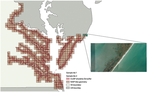
This study focuses on delineating high and low marsh communities within tidal marshes along the coast of the State of Virginia, USA. Our specific region of interest is defined as a 5-km buffer surrounding the Virginia shoreline (NOAA 2021), which is the major area marshland located in VA (see Figure 1). The majority of this coastal shoreline surrounds the Chesapeake Bay, an ecologically significant estuary that contributes to an annual economic output exceeding a hundred billion US dollars (Najjar et al. 2010; Phillips and McGee 2014).

Figure 1. Study area: shoreline (NOAA 2021) buffered with 5km distance along the state of Virginia (Runfola et al. 2020). Grid represent 2018 NAIP image tiles which intersect with the study area. Two example high-resolution NAIP imagery tiles from the eastern Delmarva Peninsula are also presented.

2.2. Imagery

2.2.1. Sentinel imagery

The Copernicus Sentinel-2 mission, launched in 2015 by the European Space Agency, provides high-resolution, multi-spectral imagery to support land monitoring studies (ESA 2018). Sentinel-2 carries 13 spectral bands with spatial resolution ranging from 10 m to 60 m, and the imagery is collected in a 5-day revisit cycle throughout the year. The 10 m RGB and NIR band (B2, B3, B4, and B8), four 20 m visible and near-infrared (VNIR) (B5, B6, B7, and B8a), and two short wave infrared bands (B11, B12) are used in this study.¹ To ensure consistent resolution across all bands, all bands originally provided at 20 m or 60 m spatial resolution were resampled to a 10 m resolution utilizing a bilinear resampling algorithm, implemented using the rasterio package in Python 3.7. This process was applied to each individual band. To account for intra-annual variability in the data, a collection of imagery was acquired for analysis, spanning different seasons in the period of 2017–2018.

2.2.2. Aerial imagery

Imagery from the National Agriculture Imagery Program (NAIP) dataset (collected by the United States Department of Agriculture (USDA)) was acquired in order to explore the value of high-resolution imagery for marsh community delineation (OCM-Partners 2022). The NAIP dataset is an aerial imagery database that has records starting in 2003 (temporal frequency of 2–3 years), sponsored through a collaboration between the United States Geological Survey (USGS) and US state governments (OCM-Partners 2022). Historically, the images were captured at 1-m spatial resolution with 4-band spectral resolution (red, green, blue, and near-infrared) across the continental United States during the agricultural growth season. Since 2018, the US state of Virginia – covering the majority of our study area – additionally began providing NAIP imagery with a resolution of 0.6 m. In this study, we use both 1-m and 0.6-m resolution NAIP imagery, spanning from 2014 to 2018. Of note, NAIP imagery is acquired during “leaf-on” time periods, leading to potential seasonal biases in acquisitions; we discuss the implications of this on model performance in the discussion.

2.2.3. Other ancillary information

Beyond the visual band information, during the training and testing phases, we also incorporated two satellite indices – NDVI and NDWI – into the network, acknowledging their historical significance in wetland classification (Sun, Fagherazzi, and Liu 2018).

2.3. Annotation resources

2.3.1. Tidal marsh inventory (TMI)

To label where marshes are located (i.e. the binary presence or absence of any type of marsh), we use the Virginia Tidal Marsh Inventory (TMI) (CCRM 2019b). The TMI is a comprehensive inventory of shoreline conditions for tidal marsh localities. The inventory relies on field workers to manually delineate marsh boundaries via a GPS-enabled system. Each marsh boundary is later digitized using the latest available high-resolution imagery from the Virginia Base Mapping Program.

2.3.2. Marsh habitat zonation map

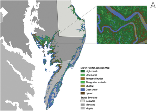
The Marsh Habitat Zone Map (MHZM) (Correll et al. 2019; SHARP 2017) is used to label imagery for high marsh and low marsh detection (expanding on the binary marsh/no marsh identification provided by TMI). The MHZM is a raster layer denoting salt marsh communities in the North Atlantic coast of the US, from northern Maine to Virginia, at a resolution of 3 m. It includes eight types of marsh communities: high marsh, low marsh, salt pool, terrestrial border, Phragmites australis (reed grass), mudflat, open water, and upland. The MHZM is subdivided into different ecological zones representing various geographic locations. For this study, zones that cover the eastern Delmarva Peninsula and the eastern shore of the Chesapeake Bay are selected to initialize a deep learning model for high marsh and low marsh feature detection (Figure 2).

Figure 2. Visualization of MHZM data covering the eastern Delmarva Peninsula and the eastern shore of the Chesapeake Bay.

2.3.3. Chesapeake Bay National Estuarine Research Reserve (CBNERR)

One challenge with both TMI and MHZM is the relatively coarse granularity of the products (due to their relatively broad geographic scopes). In order to fine-tune and validate our model using high-resolution, locally collected information, we leverage landcover maps of two NOAA National Estuarine Research Reserves (NERRs) in Virginia, the Goodwin islands and Catlett islands (Lerberg 2021). Both NERRs include detailed land cover types collected from fieldwork and digitized from high-resolution imagery by the Chesapeake Bay National Estuarine Research Reserve in Virginia (CBNERR-VA). The Goodwin islands, located on the southern side of the mouth of the York River, are a 777-acre archipelago of islands dominated by salt marshes, inter-tidal flats, and shallow open estuarine waters (Lerberg 2021). The salt marsh vegetation is dominated by Spartina alterniflora (low marsh) and Spartina patens (high marsh) and estuarine scrub/shrub vegetation in the forested wetland ridges. The Catlett Islands encompass 690 acres and display a ridge-and-swale geomorphology. The islands consist of multiple parallel ridges of forested wetland hammocks, forested upland hammocks, emergent wetlands, and tidal creeks surrounded by shallow sub-tidal areas that once supported beds of submerged aquatic vegetation. The smooth cordgrass (Spartina alterniflora) prevails over much of the marsh area along with salt grass (Distichlis spicata), saltmeadow cordgrass (Spartina patens), black needlerush (Juncus roemerianus), and various halophytic forbs (Lerberg 2021). In this study, the data from Catlett Islands is used for model fine-tuning, while the Goodwin Islands’ land cover is used to construct a dataset for independent model validation (i.e. information from the Goodwin Islands is only used for validation, and never used in model training, providing a completely external validation dataset).

2.3.4. Validation data acquisition from UAV flight

As an additional source for a fully independent validation of the presented models, two separate Unmanned Aerial Vehicle (UAV) surveys were conducted over Captain Sinclair and Maryus, Virginia, in November of 2022. The target site aerial imagery was acquired using DJI phantom-4 Multispectral drones. Filming was conducted at a 100 m altitude, primarily close to noon to minimize the impact of shadows. The orthographic image was generated by mosaicking the captured image tiles using Pix4Dmapper software (PIX4D 2022). These two sets of aerial drone imagery were employed to create an additional validation dataset for model predictions.

2.4. Data labeling procedures

The modeling procedures outlined in section 3 require a number of labeled datasets (see Table 1 for an overview of each model and the labeled datasets employed and Table 2 for a more detailed description of each tuned model):

1. Data for Marsh/No Marsh identification. We construct an independent model to identify the location of the marshland before categorizing it into high/low marsh; this requires labeled data sourced from the Tidal Marsh Inventory (TMI), and seasonal multi-band satellite imagery sourced from Sentinel-2.

2. Data for Partial Tuning. We implement an initial tuning of a model based on ImageNet (Deng et al. 2009) using data labeled with the MHZM dataset for high marsh and low marsh classification.

3. Data for Full Tuning. We implement a secondary tuning using labeled data from a local island, Catlett, sourced from CBNERR for high marsh and low marsh classification.

4. Data for Validation. Finally, we validate our models using two independently labeled dataset from (1) Goodwin Islands, sourced from CBNERR, and (2) Captain Sinclair and Maryus, Virginia, collected by UAV.

Table 1. Data source summary.

Model Name	Label Source	Label Data Type	Imagery	Imagery Resolution (meters)	Image Patches (counts)
Marsh Binary	Tidal Marsh Inventory (TMI)	vector polygons	Sentinel-2 (10m)	10	2837
Partical Tuning	Marsh Habitat Zonation Map (MHZM)	raster (3-m)	NAIP (1m)	1	10,060
Full Tuning	Catlett Islands (CBNERR)	vector polygons	NAIP (0.6m)	0.6	103
Validation	Goodwin Islands (CBNERR)	vector polygons	NAIP (0.6m)	0.6	106
Validation	Captain Sinclair & Maryus (UAV)	vector points	UAV	NA	300

Table 2. Data and model summary.

				Training Dataset(s)		Validation Dataset
Model Name	Target Classification	Description	Weights Initialization	Label Source	Imagery	Label Source	Imagery
Marsh Binary	Marsh/No marsh	U-Net w/ResNet34	ImageNet	Tidal Marsh Inventory (TMI; 70% split)	Sentinel-2 (10m resolution)	Tidal Marsh Inventory (TMI; 30% Split)	2837 Image Patches
Baseline	High/Low/No marsh	U-Net w/original Encoder/Decoder	Random	Catlett Islands (CBNERR)	NAIP (0.6m resolution)	Goodwin Islands (CBNERR)	106 Image Patches (~6.9M 0.6m Pixels)
Partial Tuning	High/Low/No marsh	U-Net w/ResNet34	ImageNet	Marsh Habitat Zonation Map (MHZM)	NAIP (1m resolution)	Goodwin Islands (CBNERR)	106 Image Patches (~6.9M 0.6m Pixels)
Full Tuning	High/Low/No marsh	U-Net w/ResNet34	ImageNet	Stage 1) MHZH Stage 2) Catlett Islands (CBNERR)	Stage 1) NAIP (1m resolution) Stage 2) 103 Image Patches (~6.M 0.6m Pixels)	Goodwin Islands (CBNERR)	106 Image Patches (~6.9M 0.6m Pixels)
Masked	High/Low/No marsh	Full Tuning Model w/Marsh Binary mask	N/A	N/A	N/A	Goodwin Islands (CBNERR)	106 Image Patches (~6.9M 0.6m Pixels)

Each of our modeling stages requires independent labeled datasets; the rest of this section details how these labeled datasets were constructed.

2.4.1. Labeling to support marshland binary modeling

The first stage of labeling is designed to provide labels to train a model which establishes the binary presence or absence of marshland. To construct these labels, we leverage 10-m resolution seasonal Sentinel-2 imagery and TMI data for labeling. The re-sampled 10-m resolution Sentinel-2 imagery is first cropped into a series of $128\times 128$ image patches, each of which has a dimension of $128\times 128\times 10$ (with 10 representing the number of bands). The TMI vector file is then overlapped with each image patch to create its corresponding labeling mask, with pixels covered by TMI boundaries labeled with value 1 representing marsh presence, and non-overlapped pixels labeled with value 0 representing marsh absence. This process results in 2,837 $128\times 128\times 10$ image patches that are used to train and test the binary marsh detection model.

2.4.2. Labeling to support partial tuning

The second stage of labeling is implemented with 1-m resolution NAIP imagery and MHZM data to construct a dataset for marsh community classification (specifically, high and low marshes). To improve compatibility with NAIP, the MHZM was first re-sampled from 3-m resolution to 1-m resolution using the nearest neighbor method. The re-sampled MHZM raster layer is then overlapped with the 1-m resolution NAIP imagery to generate a label mask; community types other than high marsh and low marsh are grouped into one background category, thus yielding a raster layer, with labels including high marsh, low marsh, and “background.”

After creating the labeled mask layer, a series of $256\times 256$ image patches are generated from the mask labels and the corresponding NAIP imagery. To ensure a reasonable number of sampling locations representing the two marsh types, we retained image patches if the $256\times 256$ pixel window contained at least 25% pixels marked either high marsh or low marsh type pixels, resulting in a dataset of 10,060 $4\times 256\times 256$ (4 is the number of image bands) tiles covering the eastern shore of the Chesapeake Bay and eastern Delmarva peninsula. This data is used to construct training datasets for the partial tuning model to learn features from high marsh, low marsh, and no marsh types.

2.4.3. Labeling to support full tuning

The third stage of labeling leverages 0.6-m resolution NAIP imagery from 2018 and high-resolution land cover maps from the Catlett Islands in VA. These images are used to further fine-tune the model. The NAIP tiles that cover the Catlett Islands were first retrieved and cropped into a series of $4\times 256\times 256$ image patches, and then these image patches are overlapped with the land cover types from CBNERRs to create the paired label patches. Within the label patches, all pixels that are not labeled as high marsh or low marsh are labeled as background (i.e. non-marsh). This process results in 103 $256\times 256$ image patch pairs for model fine-tuning, and we refer to these image patches generated from Catlett Islands as the full-tuning dataset in later sections.

2.4.4. Labeling to support external validation

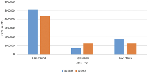
Finally, to externally validate the model, we leverage two independently collected datasets. The first of these is a stand-alone dataset from Goodwin Islands in VA. The same image processing procedures applied to Catlett Islands (our full tuning dataset) are also applied to the land cover maps of Goodwin Islands and NAIP imagery to generate patch pairs for validation. The validation image patches include 106 $4\times 256\times 256$ tiles covering Goodwin Islands, which includes 1,260,771 0.6-m resolution pixels representing high marsh, 1,277,593 pixels representing low marsh, and 4,408,452 pixels representing background. We refer to these image patches generated from the Goodwin Islands as the validation dataset in later sections.

The second independent validation dataset we employ is generated through visual interpretation of UAV imagery collected from Captain Sinclair and Maryus, Virginia. Initially, we identified and digitized a series of polygons representing land cover categories such as Juncus roemerianus, Spartina alterniflora, forest, water, and built-up areas. Subsequently, we randomly generated points within these digitized polygons using the open-source software QGIS (QGIS 2023). Each point underwent further interpretation to ensure data quality and was categorized into one of the three classes: high marsh, low marsh, or background. This process yielded a total of 300 points, comprising 158 for high marsh, 95 for low marsh, and 47 for background points. These points are used in conjunction with 106 validation image patches to generate model estimates and provide another external measurement of validity.

3. Methods

This study relies on a common procedure in the deep learning literature, transfer learning, which seeks to improve the performance of target models within specific domains by harnessing knowledge derived from distinct yet related source domains. This approach mitigates the need for an extensive amount of target domain data to construct effective target models (Zhuang et al. 2020). In this work, we train a U-Net model using a domain which has a large amount of information (data from the Delmarva Peninsula [MHZM]), and then “transfer” the weights learned in that region to our target domain by fully-tuning the model using a much smaller dataset from the Catlett Island (CBNERR). The overall workflow of this study is implemented in the following stages:

1. Leveraging the seasonal Sentinel imagery (Section 2.2.1) and digitized labels from the TMI, a binary (marsh vs. non-marsh) detection model, $M_A$, was trained over the entirety of coastal Virginia.

2. Leveraging NAIP imagery and label data from the MHZM, model $M_B$ was trained for the detection of high vs. low marsh. This step is referred to as partial tuning.

3. Initialization with the weights learned from partial tuning, $M_B$ is further fine-tuned with the in-situ high-resolution CBNERR data, generating a new model $M_C$. This step is referred to as full tuning.

4. Within areas identified as marshland by model $M_A$, model $M_C$ is implemented to discriminate between low and high marsh. This step is referred to as the masked model.

3.1. Models

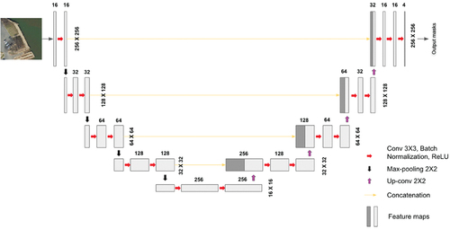
The primary algorithm used in this analysis is the U-Net, which is a well-established, relatively lightweight deep learning algorithm for semantic segmentation based on convolutional network architectures (Ronneberger, Fischer, and Brox 2015). The algorithm’s architecture includes two parts: down-sampling and up-sampling, also called the encoder and decoder. The encoder extracts varying resolution feature maps through a series of convolutional, rectified linear units (ReLU), and max-pooling layers. The decoder stage contains and combines (a) each feature map from the down-sampling process, and (b) spatial information through an up-sampling and concatenation process (Figure 3). The data flow of down-sampling and up-sampling forms a U-shaped architecture, and the output layer maintains the same resolution as the input layers.

Figure 3. The U-Net architecture (example of a 3-band input image with $256\times 256$ pixel-size) (Lv et al. 2023). The boxes indicate the feature maps at each layer, and the number on the top of each feature map shows the depth of feature map (channel). Numbers on the right side of each feature map are image/feature maps dimension.

3.1.1. Binary marsh modeling

In the binary marsh modeling $M_A$ stage, an U-Net model architecture with a Resnet-34 convolutional model is implemented to handle the encoding and decoding tasks. The model is initialized with weights pretrained with ImageNet (Deng et al. 2009). It takes 70% of the 2837 $12\times 128\times 128$ (10 spectral bands, NDVI and NDWI) image patches from Sentinel-2, and generates two types of pixel-level outputs: marsh and non-marsh. 30% of the image patches are later used to validate the model prediction accuracy (Abdi 2020; Campos-Taberner et al. 2020).

3.1.2. Partial tuning modeling

Once the location of the marshland is identified using model $M_A$, we seek to further classify the marsh as either “high” or “low”; the model presented in this subsection ($M_B$) provides the baseline for this step. Model $M_B$ is comprised of a separate U-Net model with Resnet-34 as backbone.² Network $M_B$ is then trained with 70% of the image patches from NAIP and MHZM (7042 patches). In this application, the model classifies each pixel as one of three types: high marsh, low marsh, and background (non-marsh).

3.1.3. Full tuning modeling

In the full tuning ($M_C$) model, a Resnet-34 U-Net is initialized using the optimal weights found in model $M_B$, and further trained with imagery collected from ground-truth by CBNERR (Catlett Islands). As in model $M_B$, each pixel is classified as high marsh, low marsh, or background. In this stage, all 103 $6\times 256\times 256$ image patches from CBNERR are used to train the model. The best performing model is saved for further investigation and validation.

3.1.4. Masked modeling

The masked modeling stage is a combination of the binary marsh detection model $M_A$ and the full tuning model $M_C$ results. In this stage, the $M_A$ is first leveraged to extract locations where the marshland has been detected. Within the areas identified as marshland, the $M_C$ is then leveraged to further classify the high-resolution NAIP imagery into different marsh types.

3.2. Data augmentation

In each training stage, we employ data augmentation techniques to enhance the standardization of the model input and augment the variability of the data observed by the model. To achieve standardization, we normalized the multispectral band within each image patch by dividing each band value by the maximum band value, resulting in a range between 0 and 1 for each band. As part of the data augmentation process, we generated the NDVI and NDWI bands for each image patch prior to inputting them into the model. Consequently, a total of six bands were used as inputs for model training, validation, and testing when employing NAIP imagery. In order to introduce greater diversity within the training images, we also applied morphological augmentation by randomly rotating the training images and their corresponding labels by 0, 90, 180, or 270 degrees.

3.3. Optimization & loss

In this study, we implement a multi-class cross-entropy loss function to evaluate the algorithm performance for each model described in section 3. The loss function is defined as:

(1) $loss=-\sum _{c=1}^N{y}_{o,c}log(p_{o,c})$(1)

where $N$ is the total number of mapping objects ($N$ = 2 in the model $M_A$ detecting marsh from Sentinel imagery, and $N$ = 3 in $M_B$ and $M_C$ with high and low marsh detection) and $y$ is the binary indicator (0 or 1) if class label $c$ is the correct classification for observation, $o$. $p$ is the predicted probability observation $o$ is of class $c$. Due to the imbalance of our pixel-level data distribution, a weighting scheme is used in the training process, in which classes are weighted according to their representation in the labeled data (Kikaki et al. 2022; Paszke et al. 2016):

(2) $W_{class}=\frac{1}{ln(c+p_{class})}$(2)

where $W_{class}$ is a multiplicative weight applied to the loss function for observations of a given class, $c$ is a hyper-parameter set to 1.03 (following past literature; see Kikaki et al. (2022)), and

(3) $p_{class}=\frac{N_{\mathrm{p}\mathrm{i}\mathrm{x}\mathrm{e}\mathrm{l}\mathrm{s}\mathrm{o}\mathrm{f}\mathrm{c}\mathrm{l}\mathrm{a}\mathrm{s}\mathrm{s}}}{N_{\mathrm{t}\mathrm{o}\mathrm{t}\mathrm{a}\mathrm{l}\mathrm{p}\mathrm{i}\mathrm{x}\mathrm{e}\mathrm{l}\mathrm{s}}}$(3)

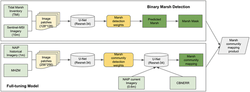
where $N_{\mathrm{t}\mathrm{o}\mathrm{t}\mathrm{a}\mathrm{l}\mathrm{p}\mathrm{i}\mathrm{x}\mathrm{e}\mathrm{l}\mathrm{s}}$ includes background pixels. During the training process, the Adam optimization is used to minimize the cross-entropy loss with an initial learning rate of 0.001. The learning rate is reduced by a factor of 10 when the models do not show any progress in validation performance for five consecutive epochs. To help avoid over-fitting, we use the best-scoring model after early stopping conditioned on no improvement in validation accuracy for 10 consecutive epochs. The overall workflow of the model process can be seen in Figure 4.

Figure 4. The workflow of the mapping process.

3.4. Accuracy assessment

We implement a wide range of validation metrics to assess pixel-level semantic segmentation performance. First and foremost, we present overall accuracy (Equation (4)(4) $\mathrm{A}\mathrm{c}\mathrm{c}\mathrm{u}\mathrm{r}\mathrm{a}\mathrm{c}\mathrm{y}=\frac{TP+TN}{TP+TN+FP+FN}$(4) ) to give guidance on the overall performance a user might expect. In addition, we evaluate the precision (Equation (5)(5) $\mathrm{P}\mathrm{r}\mathrm{e}\mathrm{c}\mathrm{i}\mathrm{s}\mathrm{i}\mathrm{o}\mathrm{n}=\frac{TP}{TP+FP}$(5) ) and recall (Equation (6)(6) $\mathrm{R}\mathrm{e}\mathrm{c}\mathrm{a}\mathrm{l}\mathrm{l}=\frac{TP}{TP+FN}$(6) ) at the pixel level for each class and the overall $F_1$ score (Congalton and Green 2019; Rwanga and Ndambuki 2017).

(4) $\mathrm{A}\mathrm{c}\mathrm{c}\mathrm{u}\mathrm{r}\mathrm{a}\mathrm{c}\mathrm{y}=\frac{TP+TN}{TP+TN+FP+FN}$(4)

(5) $\mathrm{P}\mathrm{r}\mathrm{e}\mathrm{c}\mathrm{i}\mathrm{s}\mathrm{i}\mathrm{o}\mathrm{n}=\frac{TP}{TP+FP}$(5)

(6) $\mathrm{R}\mathrm{e}\mathrm{c}\mathrm{a}\mathrm{l}\mathrm{l}=\frac{TP}{TP+FN}$(6)

(7) $F_1=\frac{2\ast Precision\ast Recall}{Precision+Recall}$(7)

In Equations (4)(4) $\mathrm{A}\mathrm{c}\mathrm{c}\mathrm{u}\mathrm{r}\mathrm{a}\mathrm{c}\mathrm{y}=\frac{TP+TN}{TP+TN+FP+FN}$(4) , (5(5) $\mathrm{P}\mathrm{r}\mathrm{e}\mathrm{c}\mathrm{i}\mathrm{s}\mathrm{i}\mathrm{o}\mathrm{n}=\frac{TP}{TP+FP}$(5) ), (6(6) $\mathrm{R}\mathrm{e}\mathrm{c}\mathrm{a}\mathrm{l}\mathrm{l}=\frac{TP}{TP+FN}$(6) ) and (7(7) $F_1=\frac{2\ast Precision\ast Recall}{Precision+Recall}$(7) ), TP (true positive) represents the number of pixels in which the model correctly predicts ground truth, TN (true negative) represents outcomes in which the model correctly predicts cases that are different than ground truth, FP (false positive) is predictions to a class that do actually not belong to that class, and FN (false negative) are the number of predictions belonging to a class but were predicted to be in a different class (Rwanga and Ndambuki 2017). The $F_1$ score is a harmonic mean between precision and recall. Finally, a cross-validation matrix (Congalton and Green 2019) for each model is additionally generated to compare the prediction accuracy for each type of marsh class.

4. Results & analysis

The results of binary detection of tidal marshes with Sentinel imagery are presented in Table 3; the results of the classification of the marsh community (high marsh vs. low marsh) are presented in Table 5. We further explain each result in the following sections.

Table 3. Accuracy assessment of binary marsh detection with Sentinel imagery and TMI (pixel-level).

		Prediction Classes
Actual Classes		Non-marsh	Marsh	Sum	Recall (%)
	Non-marsh	11,664,832	541,468	12,206,300	0.96
	Marsh	203,882	1,548,986	1,752,868	0.88
	Sum	11,868,714	2,090,454
	Precision	0.98	0.74
	Overall Accuracy	0.95	Overall $F_1$	0.89

Table 4. Accuracy assessment of binary marsh detection with NAIP imagery and TMI (pixel-level).

		Prediction Classes
Actual Classes		Non-marsh	Marsh	Sum	Recall (%)
	No-marsh	54,909,848	3,996,778	58,906,626	0.93
	Marsh	2,025,841	9,977,485	12,003,326	0.83
	Sum	56,935,689	13,974,263
	Precision	0.96	0.71
	Overall Accuracy	0.92	Overall $F_1$	0.86

Table 5. Accuracy assessment results tested using all data from the Goodwin Islands. Four prediction results are presented: baseline model, direct prediction from partial tuning, full tuning, and masked modeling. Each tested class is presented with two statistics: precision and recall. Each model is presented with overall accuracy and $F_1$ score.

		Background	High Marsh	Low Marsh	Overall Accuracy	$F_1$
Baseline	Precision	0.99	0.31	0.5	0.63	0.52
	Recall	0.77	0.98	0.15
Partial Tuning	Precision	0.98	0.34	0.47	0.66	0.48
	Recall	0.88	0.95	0.01
Full Tuning	Precision	0.99	0.71	0.66	0.85	0.81
	Recall	0.84	0.91	0.82
Masked Modeling	Precision	0.96	0.77	0.74	0.88	0.83
	Recall	0.91	0.85	0.79

4.1. Model performance of sentinel marsh detection

Table 3 provides a pixel-level accuracy assessment, based on a randomized 30% split of Sentinel data withheld for validation. Out of the 2,090,454 pixels predicted as marsh by the model, 1,548,986 pixels are marsh according to the validation data. This accounts for 74% of the pixels labeled as marsh. Out of the total 1,752,868 pixels labeled as marsh in the ground truth data, the model correctly identifies 1,548,986 of them as marsh, which corresponds to 88%. The model achieves an overall accuracy of 95% and an overall $F_1$ score of 0.89.

To test whether spatial resolution would improve or impede the model performance in marsh detection, we construct another dataset with the 0.6-m resolution NAIP and TMI labels. The results (based on a withheld subset of 30% of the data) are presented in Table 4. The prediction accuracy for the marsh and non-marsh detections is 71% and 96%, respectively. The recalls for the two classes – marsh and non-marsh – are 83% and 93%. Using high spatial resolution NAIP imagery, the model achieves 92% overall accuracy and an overall $F_1$ score of 0.86 (a small decrease from the sentinel models presented in Table 3).

4.2. Model performance and accuracy of marsh community mapping

Here, we present the results of our models designed to distinguish between high and low marsh (as described in sections 3.1.2, 3.1.3 and 3.1.4).

The models are each initially tested using a stand-alone testing dataset representing the Goodwin Islands (an area intentionally omitted from any training stage; see section 2.3); later in this section we provide results from an additional, independent UAV survey. Results from the Goodwin Islands are summarized in Table 5.³

The first model presented in Table 5 (the “Baseline Model”) provides a baseline as to the accuracy that might be expected if a researcher only used one locally collected dataset (Catlett Islands) to tune the model. As anticipated, this approach has poor performance in predicting both high marsh and low marsh, with 31% and 50% precision, respectively. Although the prediction accuracy for the non-marsh type (background) is 99%, the recall is only 77%, meaning 23% of the background pixels in the ground truth are mis-classified as marsh (i.e. overestimating the amount of marshland in the prediction). Considering that the number of background pixels in the testing dataset make up more than 50% of the entire testing set (see Figure 5), this is a large discrepancy at the pixel level. This baseline method achieves 63% overall accuracy and an overall $F_1$ score of 0.52.

Figure 5. The distribution of data used in full-tuning and validation. The blue bars are the number of pixels counts calculated from the full-tuning dataset, and the orange bars are pixel counts from the validation dataset (in Section 2.3).

The second model presented in Table 5 - the “Partial Tuning” model – is also tested using the stand-alone validation dataset. In this model, we are training based on the relatively coarse-resolution, but data rich Marsh Habitation Zonation Map (MHZM), but without any further training with in-situ collected data. Similar to the baseline model, partial tuning results in relatively poor performance in predicting all three categories, with a 66% overall accuracy and a $F_1$ score of 0.48.

The next model presented in Table 5 - the “full tuning” model – sought to establish the improvement in accuracy that may be possible given the in-situ collection of small amounts of high-quality data. The full tuning model improves the model performance dramatically, with 22% and 29% improvement in overall accuracy and $F_1$ score, respectively. The prediction accuracy of high marsh and low marsh increased from 0.31 to 0.71, and from 0.50 to 0.66, respectively. Although there is a slight decrease in recall in high marsh prediction (from 0.98 to 0.91), the recall of low marsh is increased from 0.15 to 0.82. The recall value for the background increased 7% (from 77% to 84%). This leads to a significant improvement in the model’s overall performance on each land cover category.

In the final model implementation (“masked model”), we first leverage the binary marsh model to mask regions for consideration, and then apply the full tuning model for high and low marsh identification to the resultant area. This model improves the overall accuracy by 3% and $F_1$ score by 2%. The model precision in predicting high marsh and low marsh increased by 6% and 8%, respectively.

Overall, there is a 25% improvement in overall accuracy and 31% improvement in $F_1$ score between the baseline model and the final masked model (with full tuning and marsh presence detection). The difference in precision is 46% and 24% for high marsh and low marsh, respectively. No particular class correlates closely with overall performance. Figure 6 shows the comparison of different prediction results, compared with ground truth labeling.

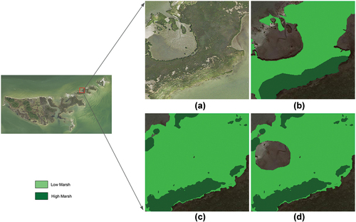
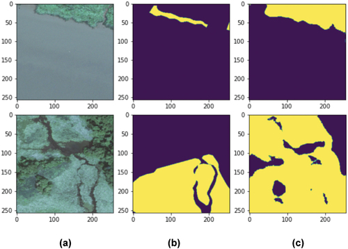
Figure 6. A visualization of model prediction in a selected area in the validation region (Goodwin Islands). A) the raw NAIP imagery (0.6-m spatial resolution); B) ground truth label; C) prediction output of full tuning model; D) prediction output of masked model.

To validate the robustness of the model predictions, Table 6 summarizes the results for data interpreted from UAV imagery using the masked modeling technique. The model exhibits an overall accuracy of 79% in predicting these samples. The model achieves a prediction accuracy of 73% and 93% for high marsh and low marsh, respectively. Notably, the recall value of high marsh is 98%, while the recall value of low marsh is 43%.

Table 6. A summary of the accuracy assessment results obtained from the masked modeling approach using UAV-interpreted data collected in Captain Sinclair and Maryus, Virginia.

	Precision	Recall	F1	Total
Background	0.98	0.89	0.93	47
High Marsh	0.73	0.98	0.84	158
Low Marsh	0.93	0.43	0.59	95
Overall Accuracy	0.79

4.3. Error distribution across space

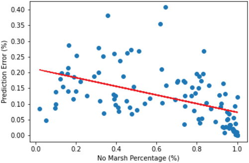
To explore the potential bias in the spatial distribution of errors (and thus provide a better understanding of which features may correlate with accuracy or inaccuracy), we generated a spatially gridded metric of error, which is presented in Figure 7. Each grid cell in this figure shows the overall percentage of misclassified pixels in the underlying validation dataset. As this figure illustrates, in regions with more complex land cover mixtures, the prediction error tends to be higher compared to regions with more homogeneous or distinct land cover types. We also find a relationship between an increased percentage of non-marsh in image patches and the total amount of error; broadly, as non-marsh areas increase, error tends to decrease, as shown in Figure 8.

Figure 7. Prediction error of each patch (Goodwin Islands).

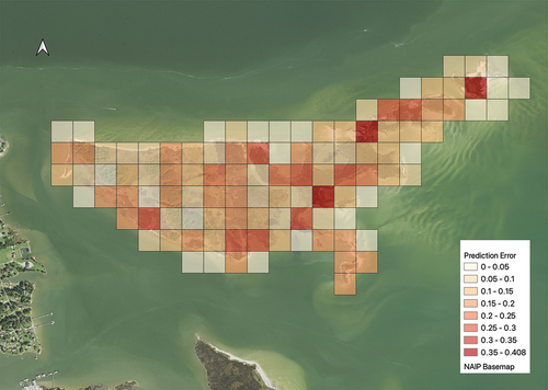
Figure 8. The relationship between prediction error and the percentage of no marsh type of images patches in the validation data.

5. Discussion

The overall results of this study illustrate that leveraging features learned from locations where data are abundant, the classification accuracy of marsh types – high marsh, low marsh, and non-marsh – can reach approximately 85% in the Virginia study area. The combination of data from multiple sources with various spatial resolutions – Sentinel and NAIP – can improve the overall accuracy of marsh community classification to 88%. Notably, this accuracy is a pixel-level metric, i.e. the number of approximately 60-cm pixels that are classified correctly. In this section, we explore model performance and highlight a number of directions for future research.

5.1. Discrepancies across data sources

One significant issue in the approach we present in this paper is the temporal mismatch between the image and annotation data for marsh detection. The binary marsh label data (TMI) were manually collected from high-resolution images between 2010 and 2018, varying across different sites. In contrast, the input imagery consists of data from 2017 to 2018 (Sentinel with different seasonal coverages) and 2018 (NAIP collected during leaf-on periods). Consequently, in some cases, the model attempts to correlate the state of marshland at one point in time with images from another time. This temporal mismatch can have a negative effect on model performance due to changes wetlands undergo over time, due to both natural and human-driven processes (Mainali et al. 2023). This is illustrated in Figure 9, where column (B) displays tidal marsh labels from TMI; as can be seen, these labels do not precisely align with the ground truth shown in the imagery in column (A). Given this discrepancy, it is possible that our validation understates the overall accuracy of the model’s performance because the validation and calibration data itself contain apparent errors, thus influencing the overall model performance reported earlier. Interestingly, models such as those presented in this piece could potentially be employed to retrospectively improve long-term records such as those provided by TMI.

Figure 9. A visualization of samples of images with the corresponding ground truth labels using high-resolution NAIP imagery. A) the raw NAIP imagery; B) annotations from TMI; C) model prediction of marsh presence (yellow pixels are marsh).

A separate, but interrelated challenge is that the extent of marshland inundation exhibits regular temporal variability attributable to natural hydrological processes. The tidal wetland area is subject to notable alterations during storm events, as well as gradual shifts resulting from phenomena such as sea level rise and land subsidence. Unfortunately, the NAIP imagery, which serves as our primary data source for mapping the marsh communities, is collected specifically during the leaf-on season. As a result, the influence of tidal dynamics on model performance, particularly for accurately mapping low marsh areas, is neglected. To address this limitation, future endeavors could involve employing alternative high-resolution imagery sources with higher temporal frequency. However, we note that the model performance we present here is very promising, suggesting that – despite this limitation – NAIP-based modeling approaches may still be a strong pathway forward for modeling efforts focused on the United States. This is notable, as NAIP is a public good which managers or analysts can retrieve free of cost; similar products from commercial companies can easily cost tens to hundreds-of-thousands of dollars depending on the scope of data required.

5.2. Comparison of results from different sources

In the context of binary marsh detection, the optimal model achieves an overall accuracy of 95% when utilizing the multispectral seasonal imagery acquired from Sentinel-2. By employing the four-band high-resolution imagery obtained from NAIP, the model achieves an overall accuracy of 92%. The observed 3% increase in overall accuracy, attained through the utilization of Sentinel-2 imagery, can likely be attributed to the information captured by the additional spectral bands that are not available in NAIP imagery. While there is a disparity in image patch sizes between Sentinel-2 ($128\times 128$) and NAIP ($256\times 256$) during the training phase, potentially resulting in variations in model performance, the effect of image size on classification accuracy is unknown and an avenue for future research.

However, it is important to note that the NAIP dataset offers a high-resolution data source that enables the measurement of the more detailed distribution of marsh communities within the study area. This provides valuable information that cannot be obtained from Sentinel-2 imagery alone. The combination of both resources for marsh community mapping allows for leveraging the benefits of both data sources, enhancing the accuracy and detail of the mapping results.

In the context of marsh community mapping, employing partial tuning on the testing dataset results in relatively poor performance, with an overall accuracy of 66% and an F1 score of 0.48. This lower performance can be attributed to the disparity in spatial resolution between the images used for model training and testing. Specifically, the model is trained using a series of 1-m resolution NAIP imagery, while evaluation is carried out on 0.6-m resolution imagery obtained from the study area. Notably, recent research conducted by Thambawita et al. (2021) underscores the impact of image resolution on model performance, highlighting the tendency for decreased performance when generalizing to spatial resolutions outside the scope of the training dataset.

To address this limitation, conducting full tuning using 0.6-m data collected from the study area leads to a significant improvement in performance, boosting the overall accuracy from 66% to 85%. This observation may help guide future efforts: while using off-the-shelf models is not a suitable solution today, collecting relatively small amounts of local data to fine-tune existing models to different locales is an effective pathway forward, even in the context of image resolution differences between the source and target modeling domains.

5.3. Feature importance – model interpretation

A frequent criticism of deep learning models highlights the difficulty of interpreting the relative importance of features in estimation. To explore the mechanisms driving the presented models, we apply a SHAP visualization (SHapley Additive exPlanations visualization technique (Lundberg and Lee 2017)) to explore what factors contribute to the model’s capability to distinguish different marsh types. Figure 10 provides an illustrative example of the factors influencing the accurate classification of three images within the ResNet-34-based network. In Figure 10, example images are in the first column, while the second, third, and fourth columns show pixel-level features that either contribute positively (highlighted in red) or negatively (highlighted in blue) to classification into the respective categories indicated above each.

Figure 10. Three random correctly classified test images are in the first column. The second, third, and fourth columns show the pixels/features that contributed for and against classification into each of the three classes. For example, the upper-left image is a low marsh image that was predicted by the model most likely to be a low marsh, then background, then high marsh. Blue pixels represent areas that contribute against classification to a given class and red pixels represent areas that contribute toward. In this case, the Resnet-34 based network for image classification was investigated.

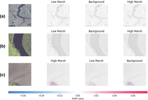
The visual examination of the SHAP examples, as illustrated in Figure 10, highlights the discernible influence of specific geographic characteristics on model classification. Notably, in Figures 10A,B, which pertain to the low marsh category, the boundary between water and land (i.e. marsh bank) exhibits a relatively high contribution compared to other surface areas in identifying low marsh regions. This contribution is represented by the presence of red-colored pixels along the shorelines. Relatedly, the final columns of the top two rows demonstrate that indicators along the shoreline exert a negative influence on the classification of high marsh. A more complex example is shown in Figure 10C, in which the true class (high marsh) is identified, but the information used for distinguishing between high marsh and low marsh shows a more diffuse pattern, i.e. contextual information is being leveraged, rather than only pixels proximate to the shoreline.

In the SHAP evaluation, because the underlying images are not themselves segmented, the SHAP values are constructed on a pixel-by-pixel basis, and thus do not inherently have semantic meanings. This study would benefit from more robust explainability techniques that identify (e.g. through natural language or generative interpretation) the most influential features affecting marsh classification.

5.4. Advantages as contrasted to alternative techniques for marsh monitoring in Virginia

Traditional tidal marsh mapping involves resource-intensive GPS field surveys and manual digitization from remotely sensed data. For instance, the most recent Tidal Marsh Inventory (TMI) for Virginia spanned a nine-year period from 2011 to 2019 (CCRM 2019b). While the TMI provides a comprehensive inventory of tidal marsh locations, it lacks detailed information about the specific spatial distribution of marsh types, such as distinguishing between high marsh and low marsh. In contrast, this study explores the application of deep learning techniques using high-resolution imagery. By leveraging these methods, we not only accurately map the marshland but also detect and differentiate marsh types, providing more detailed and comprehensive information compared to traditional approaches at significantly lower labor costs.

The proposed method in this study achieves an overall accuracy of 95% in binary marsh detection and 88% in marsh type classification for the Virginia region. The training process leverages an NVIDIA GPU Quadro RTX 6000 with 24 GB memory. After training, individual tiles (i.e. a $128\times 128$ Sentinel-2 image patch covering roughly 1,638,400m²) can be processed with estimates provided in less than a second. If these techniques can be made to generalize without local training information, the processing time for an entire study area could be decreased from years to hours.

5.5. Limitations in the use of high-resolution imagery

5.5.1. Seasonality

Tidal marshes demonstrate unique spectral attributes across diverse seasons and tidal conditions. Moreover, the spectral signatures and attributes of identical marsh types can undergo variations as a result of the influence of tidal inundation. Researchers conducting similar studies typically adhere to specific guidelines when dealing with tidal influences for analysis. For instance, some opt for images captured during low tide periods (Alam and Hossain 2021), while others have developed specialized filtering techniques to isolate the tidal influence in marsh classification studies (Sun et al. 2021).

One of the notable strengths of the U-Net architecture is its capability to learn and represent a wide range of image features that are correlated with phenomena of interest, a characteristic that proves especially advantageous in the context of regularly inundated coastal areas (Li et al. 2021). However, in the work presented in this paper, limitations arise from the utilization of publicly available high-resolution imagery, specifically NAIP, which lacks a high temporal coverage and repetitive data acquisition schedule. Consequently, the classification of high marsh and low marsh from such imagery may not fully capture the nuances of seasonal variations and tidal influences. It is important to acknowledge that this limitation is inherent to the use of publicly accessible high-resolution image sources today and cannot be entirely circumvented using open-source information. Although commercial high-resolution satellite imagery that also has temporal regularity is available from some private providers, not every government agency or environmental protection agency has the resources to make such purchases. Thus, we note that despite the inherent limitations of NAIP, the work presented in this study suggests that its use remains a viable pathway for mapping and modeling marsh types in fiscally constrained environments.

5.5.2. Shadows

Shadows stemming from cloud cover or tree canopies constitute an additional factor impacting the accurate classification of high-resolution imagery. Shaded regions frequently exhibit spectral characteristics that closely resemble those of water, primarily due to the influence of shadows cast by tree canopies, and can thus introduce significant errors into wetland detection algorithms. As the U-Net model is adept at identifying multiple features that may correlate with a feature of interest, one way to address this challenge is through the incorporation of images captured at different seasons or times.

However, in this study, we leverage NAIP, which provides only one image during a leaf-on period, suggesting that shadows may be a significant source of errors. In future studies, we suggest the integration of shadow-detection algorithms (i.e. Liasis and Stavrou (2016); Shi, Fang, and Zhao (2023)) into supplementary pre-processing stages. More generally, a fruitful avenue for future inquiry could be the integration of such shadow detection and removal strategies into the U-Net model itself.

6. Conclusion

Efforts to map tidal marshes play a crucial role in coastal resource management, offering valuable insights into the trends and overall health of essential vegetation. These data serve as a valuable resource for scientists, coastal planners, and managers, helping them identify specific areas where resources can be allocated, facilitating the implementation of monitoring, protection, and restoration initiatives aimed at enhancing the resilience of these habitats.

Despite the importance of these data, current practices of tidal marsh inventory mapping face several limitations, including the necessity for on-site data collection, manual image digitization, and restricted access to remote areas. These challenges can result in data products that are rarely – if ever – updated, a particularly detrimental factor in the context of dynamic processes like sea level rise. In this paper, our objective is to explore the capability of overhead imagery and deep learning-based segmentation models to identify marsh types – specifically, the degree to which it is possible to distinguish between high marsh and low marsh when using mixed-resolution imagery. To achieve this, we leverage multispectral Sentinel-2 imagery and high spatial resolution NAIP imagery for the classification of marsh plant communities. This study presents a benchmark accuracy of 88% for deep learning-based marsh community classification in coastal Virginia, achieved at a spatial resolution of 60 cm. Limitations arise when using static high-resolution NAIP imagery, including challenges related to tidal inundation and the influence of shadows (see section 5.5). The findings, proposed workflow, and methodology presented in this study offer a novel approach for regional governments to generate high-resolution tidal marsh inventories using only open-access imagery.

Author’s contribution

The authors confirm their contribution to the paper as follows: ZL conceptualized the project, with input from DR, EB, and KN. ZL wrote code to prepare data and implement machine learning methods, analysis, and other components. DR assisted in algorithm and methodology development. This piece was written by ZL with input from DR and EB. All authors reviewed the results and approved the final version of the manuscript.

Acknowledgments

The authors acknowledge William & Mary Research Computing for providing computational resources and technical support that have contributed to the results reported within this paper. URL: https://www.wm.edu/it/rc. Special appreciation is extended to Scott B. Lerberg and William G. Reay from the Chesapeake Bay National Estuarine Research Reserve, Virginia, for their invaluable support in CBNERR fieldwork activities and providing land cover information for Goodwin Islands and Catlett Islands. Recognition is also extended to Kory Angstadt and David Stanhope from VIMS Center for Coastal Resources Management (CCRM) for their contributions to UAV data collection. The authors would like to acknowledge Catherine Duning and Sharon Killeen from CCRM for their assistance in initial data exploration. Lastly, gratitude is extended to the anonymous reviewers and editor whose insightful comments greatly contributed to the enhancement of this manuscript.

Disclosure statement

No potential conflict of interest was reported by the author(s).

Data availability statement

The data that support the findings of this study are available from the corresponding authors, Dan Runfola and Zhonghui Lv, upon reasonable request.

Additional information

Funding

This work was supported by the National Science Foundation [2317591].

Notes

1. The B1, B9, and B10 bands were not leveraged, as they are mainly used for atmospheric correction.

2. Pretrained weights from ImageNet are used for initialization.

3. Results from a baseline model are also included by training a U-Net model with only the 103 image patches from Catlett Islands in Virginia, in order to establish the value of the more complex training procedure outlined in this piece; results from the UAV survey are presented in Table 6

References

- Abdi, A. M. 2020. “Land Cover and Land Use Classification Performance of Machine Learning Algorithms in a Boreal Landscape Using Sentinel-2 Data.” GIScience & Remote Sensing 57 (1): 1–23. https://doi.org/10.1080/15481603.2019.1650447.
- Alam, S. M. R., and M. S. Hossain. 2021. “A Rule-Based Classification Method for Mapping Saltmarsh Land-Cover in South-Eastern Bangladesh from Landsat- 8 Oli.” Canadian Journal of Remote Sensing 47 (3): 356–380. https://doi.org/10.1080/07038992.2020.1789852.
- Amani, M., M. Kakooei, A. Ghorbanian, R. Warren, S. Mahdavi, B. Brisco, and A. Moghimi, L. Bourgeau-Chavez, S. Toure, A. Paudel, A. Sulaiman. 2022. “Forty Years of Wetland Status and Trends Analyses in the Great Lakes Using Landsat Archive Imagery and Google Earth Engine.” Remote Sensing 14 (15): 3778. https://www.mdpi.com/2072-4292/14/15/3778.
- Barbier, E. B., S. D. Hacker, C. Kennedy, E. W. Koch, A. C. Stier, and B. R. Silliman. 2011. “The Value of Estuarine and Coastal Ecosystem Services.” Ecological Monographs 81 (2): 169–193. https://doi.org/10.1890/10-1510.1.
- Bhosle, K., and V. Musande. 2019. “Evaluation of Deep Learning Cnn Model for Land Use Land Cover Classification and Crop Identification Using Hyperspectral Remote Sensing Images.” The Journal of the Indian Society of Remote Sensing 47 (11): 1949–1958. https://doi.org/10.1007/s12524-019-01041-2.
- Brewer, E., J. Lin, P. Kemper, J. Hennin, D. Runfola, and T. R. Gadekallu. 2021. “Predicting Road Quality Using High Resolution Satellite Imagery: A Transfer Learning Approach.” PLOS ONE 16 (7): 1–18. https://doi.org/10.1371/journal.pone.0253370.
- Brewer, E., J. Lin, and D. Runfola. 2022. Susceptibility & Defense of Satellite Image-Trained Convolutional Networks to Backdoor Attacks. Information Sciences 603 (7): 244–261. https://doi.org/10.1016/j.ins.2022.05.004
- Campbell, A., and Y. Wang. 2019. “High Spatial Resolution Remote Sensing for Salt Marsh Mapping and Change Analysis at Fire Island National Seashore.” Remote Sensing 11 (9): 1107. https://doi.org/10.3390/rs11091107.
- Campbell, A. D., Y. Wang, and C. Wu. 2020. “Salt Marsh Monitoring Along the Mid-Atlantic Coast by Google Earth Engine Enabled Time Series.” PLOS ONE 15 (2): e0229605. https://doi.org/10.1371/journal.pone.0229605.
- Campos-Taberner, M., F. García-Haro, B. Martínez, E. Izquierdo-Verdiguier, C. Atzberger, G. Camps-Valls, and M. A. Gilabert. 2020. “Understanding Deep Learning in Land Use Classification Based on Sentinel-2 Time Series.” Scientific Reports 10 (1): 17188. https://doi.org/10.1038/s41598-020-74215-5.
- Carle, M. V., L. Wang, and C. E. Sasser. 2014. “Mapping Freshwater Marsh Species Distributions Using Worldview-2 High-Resolution Multispectral Satellite Imagery.” International Journal of Remote Sensing 35 (13): 4698–4716. https://doi.org/10.1080/01431161.2014.919685.
- Carr, J. A. I., G. A. I. Guntenspergen, and M. Kirwan. (2020). Modeling Marsh-Forest Boundary Transgression in Response to Storms and Sea-Level Rise, 47. https://www.sciencedirect.com/science/article/pii/S0169204613001345.
- Carter, V. 1981. “Remote Sensing for Wetland Mapping and Inventory.” Water International 6 (4): 177–185. https://doi.org/10.1080/02508068108685935.
- CCRM. (2019a). Field Guide to Virginia Salt and Marsh Brackish Marsh Plants. VIMS Center for Coastal Resource Management. Virginia Institute of Marine Science. http://ccrm.vims.edu/publications/pubs/8x11brochureannotated2rh.pdf.
- CCRM. (2019b). Virginia Shoreline & Tidal Marsh Inventory. VIMS Center for Coastal Resource Management. Virginia Institute of Marine Science. https://www.vims.edu/ccrm/research/inventory/virginia/index.php.
- Chaudhuri, G., and N. B. Mishra. 2023. “Detection of Aquatic Invasive Plants in Wetlands of the Upper Mississippi River from Uav Imagery Using Transfer Learning.” Remote Sensing 15 (3): 734. https://doi.org/10.3390/rs15030734.
- Congalton, R., and K. Green. 2019. Assessing the Accuracy of Remotely Sensed Data: Principles and Practices. 3rd ed. Boca Raton: CRC Press.
- Correll, M. D., W. Hantson, T. P. Hodgman, B. B. Cline, C. S. Elphick, W. G. Shriver, and E. L. Tymkiw, B. J. Olsen. 2019. “Fine-Scale Mapping of Coastal Plant Communities in the Northeastern Usa.” Wetlands 39 (1): 17–28. https://link.springer.com/article/10.1007/s13157-018-1028-3.
- Deng, J., W. Dong, R. Socher, L.-J. Li, K. Li, and L. Fei-Fei. 2009. Imagenet: A large- scale hierarchical image database. In 2009 ieee conference on computer vision and pattern recognition (pp. 248–255).
- Dewitz, J. 2021. National Land Cover Database (Nlcd) 2019 Products. U.S. Geological Survey. https://doi.org/10.5066/P9KZCM54.
- ESA. (2018). Sentinel. European Space Agency. https://sentinel.esa.int/web/sentinel/home.
- Feagin, R. A., M. L. Martínez, G. Mendoza-González, and R. Costanza. 2010. “Salt Marsh Zonal Migration and Ecosystem Service Change in Response to Global Sea Level Rise: A Case Study from an Urban Region.” Ecology and Society 15 (4). https://doi.org/10.5751/ES-03724-150414.
- Fisher, J., and M. C. Acreman. 2004. “Wetland Nutrient Removal: A Review of the Evidence.” Hydrology and Earth System Sciences 8 (4): 673–685. https://hess.copernicus.org/articles/8/673/2004/.
- FWS. (2023). National Wetlands Inventory. U.S. Fish Wildlife Service. Accessed on 2023: https://data.nal.usda.gov/dataset/national-wetlands-inventory.
- Gale, S. 2021. National Wetlands Inventory (Nwi) Accuracy in North Carolina. https://www.ncwetlands.org/wp-content/uploads/NWIAccuracyInNCNCDWR-FinalReport8-10-2021.pdf.
- Gao, Y. Y., and J.-F. Mas. 2008. A Comparison of the Performance of Pixel-Based and Object- Based Classifications Over Images with Various Spatial Resolutions.
- Goodman, S., A. BenYishay, and D. Runfola. 2021. “A Convolutional Neural Network Approach to Predict Non-Permissive Environments from Moderate- Resolution Imagery.” Transactions in GIS 25 (2): 674–691. https://doi.org/10.1111/tgis.12661.
- Guirado, E., S. Tabik, D. Alcaraz-Segura, J. Cabello, and F. Herrera. 2017. “Deep-Learning versus Obia for Scattered Shrub Detection with Google Earth Imagery: Ziziphus Lotus as Case Study.” Remote Sensing 9 (12): 1220. https://doi.org/10.3390/rs9121220.
- Homer, C., J. Dewitz, S. Jin, G. Xian, C. Costello, P. Danielson, and L. Gass, M. Funk, J. Wickham, S. Stehman, R. Auch. 2020. “Conterminous United States Land Cover Change Patterns 2001–2016 from the 2016 National Land Cover Database.” ISPRS Journal of Photogrammetry and Remote Sensing 162:184–199. https://doi.org/10.1016/j.isprsjprs.2020.02.019.
- Kang, Y., E. Jang, J. Im, and C. Kwon. 2022. “A Deep Learning Model Using Geostationary Satellite Data for Forest Fire Detection with Reduced Detection Latency.” GIScience & Remote Sensing 59 (1): 2019–2035. https://doi.org/10.1080/15481603.2022.2143872.
- Kelly, M., S. D. Blanchard, E. Kersten, and K. Koy. 11 2011. “Terrestrial Remotely Sensed Imagery in Support of Public Health: New Avenues of Research Using Object-Based Image Analysis.” Remote Sensing 3 (11): 2321–2345. https://doi.org/10.3390/rs3112321.
- Kennish, M. J. 2001. “Coastal Salt Marsh Systems in the U.S.: A Review of Anthropogenic Impacts.” Journal of Coastal Research 17:731–748. https://api.semanticscholar.org/CorpusID:128791900.
- Khanna, S., M. J. Santos, S. L. Ustin, A. Koltunov, R. F. Kokaly, D. A. Roberts, and A. A.-J. Golden. 2013. “Detection of Salt Marsh Vegetation Stress and Recovery After the Deepwater Horizon Oil Spill in Barataria Bay, Gulf of Mexico Using Aviris Data.” PLOS ONE 8 (11): e78989. https://doi.org/10.1371/journal.pone.0078989.
- Kikaki, K., I. Kakogeorgiou, P. Mikeli, D. E. Raitsos, K. Karantzalos, and B. K. Veettil. 2022. “Marida: A Benchmark for Marine Debris Detection from Sentinel- 2 Remote Sensing Data.” PLOS ONE 17 (1): e0262247. https://doi.org/10.1371/journal.pone.0262247.
- Krizhevsky, A., I. Sutskever, and G. Hinton. 2012. “Imagenet Classification with Deep Convolutional Neural Networks.” Neural Information Processing Systems 25 (1): 84–90. https://doi.org/10.1145/3065386.
- Lamb, B. T., M. A. Tzortziou, and K. C. McDonald. 10 2019. “Evaluation of Approaches for Mapping Tidal Wetlands of the Chesapeake and Delaware Bays.” Remote Sensing 11 (20): 2366. https://doi.org/10.3390/rs11202366.
- Lerberg, S. 2021. Goodwin Islands and Catlett islands high resolution land cover mapping products. Produced using Garfield, N., K. Madden, S. Upchurch, S. Shull, N. Herold, M. Ferner, and C. Weidman. 2013. Mapping Land Use and Habitat Change in the NERRS: Standard Operating Procedures: Version 2. Amended May 2015. Companion Document to: Recommended Guidelines for Adoption and Implementation of the NERRS Comprehensive Habitat and Land Use Classification System. Silver Spring, MD: Report for the National Estuarine Research Reserves System, NOAA/NOS/OCM.
- Liasis, G., and S. Stavrou. 2016. “Satellite Images Analysis for Shadow Detection and Building Height Estimation.” ISPRS Journal of Photogrammetry and Remote Sensing 119:437–450. https://doi.org/10.1016/j.isprsjprs.2016.07.006.
- Liu, M., B. Fu, D. Fan, P. Zuo, S. Xie, H. He, and L. Liu, L. Huang, E. Gao, M. Zhao. 2021. “Study on Transfer Learning Ability for Classifying Marsh Vegetation with Multi-Sensor Images Using Deeplabv3+ and Hrnet Deep Learning Algorithms.” International Journal of Applied Earth Observation and Geoinformation 103:102531. https://doi.org/10.1016/j.jag.2021.102531.
- Liu, D., and F. Xia. 2010. “Assessing Object-Based Classification: Advantages and Limitations.” Remote Sensing Letters 1 (4): 187–194. https://doi.org/10.1080/01431161003743173.
- Li, H., C. Wang, Y. Cui, and M. Hodgson. 2021. Mapping salt marsh along coastal south carolina using u-net. ISPRS Journal of Photogrammetry and Remote Sensing 179 (9): 121–132. https://doi.org/10.1016/j.isprsjprs.2021.07.011
- López-Tapia, S., P. Ruiz, M. Smith, J. Matthews, B. Zercher, L. Sydorenko, and N. Varia, Y. Jin, M. Wang, J. B. Dunn, A. K. Katsaggelos. 2021. “Machine Learning with High-Resolution Aerial Imagery and Data Fusion to Improve and Automate the Detection of Wetlands.” International Journal of Applied Earth Observation and Geoinformation 105:102581. https://doi.org/10.1016/j.jag.2021.102581.
- Lundberg, S., and S.-I. Lee. 2017. A Unified Approach to Interpreting Model Predictions. arXiv. https://arxiv.org/abs/1705.07874.
- Lv, Z., K. Nunez, E. Brewer, and D. Runfola. 2023. “Pyshore: A Deep Learning Toolkit for Shoreline Structure Mapping with High-Resolution Orthographic Imagery and Convolutional Neural Networks.” Computers & Geosciences 171 (105296): 105296. https://doi.org/10.1016/j.cageo.2022.105296.
- Mainali, K., M. Evans, D. Saavedra, E. Mills, B. Madsen, and R. Minnemeyer. 2023. “Convolutional Neural Network for High-Resolution Wetland Mapping with Open Data: Variable Selection and the Challenges of a Generalizable Model.” Science of the Total Environment 861:160622. https://doi.org/10.1016/j.scitotenv.2022.160622.
- Matthews, J. W., D. Skultety, B. Zercher, M. P. Ward, and T. J. Benson. 2016. “Field verification of original and updated national wetlands inventory maps in three metropolitan areas in Illinois, usa.” Wetlands 36 (6): 1155–1165. https://doi.org/10.1007/s13157-016-0836-6.
- Miller, C. B., A. B. Rodriguez, and M. C. Bost. 2021. “Sea-Level Rise, Localized Subsidence, and Increased Storminess Promote Saltmarsh Transgression Across Low- Gradient Upland Areas.” Quaternary Science Reviews 265:107000. https://doi.org/10.1016/j.quascirev.2021.107000.
- Morgan, G. R., C. Wang, Z. Li, S. R. Schill, and D. R. Morgan. 2022. “Deep Learning of High-Resolution Aerial Imagery for Coastal Marsh Change Detection: A Comparative Study.” ISPRS International Journal of Geo-Information 11 (2): 100. https://doi.org/10.3390/ijgi11020100.
- Mukherjee, R., and D. Liu. 2021. “Downscaling Modis Spectral Bands Using Deep Learning.” GIScience & Remote Sensing 58 (8): 1300–1315. https://doi.org/10.1080/15481603.2021.1984129.
- Murray, N. J., T. A. Worthington, P. Bunting, S. Duce, V. Hagger, C. E. Lovelock, and M. B. Lyons. 2019. “High-Resolution Mapping of Losses and Gains of Earth’s Tidal Wetlands.” .
- Najjar, R. G., C. R. Pyke, M. B. Adams, D. Breitburg, C. Hershner, M. Kemp, and R. Wood. 2010. “Potential Climate-Change Impacts on the Chesa- Peake Bay.” Estuarine, Coastal and Shelf Science 86 (1): 1–20. https://www.sciencedirect.com/science/article/pii/S0272771409004582.
- Narayan, A., E. Tuci, F. Labrosse, and M. H. M. Alkilabi. 2017, 9. Road Detection Using Convolutional Neural Networks. Proceedings of the 14th European Conference on Artificial Life ECAL 2017, 314–321. https://www.mitpressjournals.org/doi/abs/10.1162/isala053.
- NOAA. (2021). NOAA Continually Updated Shoreline Product (Cusp). Accessed March , 2022. https://shoreline.noaa.gov/data/datasheets/cusp.html.
- NOAA. 2023. Coastal Change Analysis Program (C-Cap) High-Resolution Land Cover. NOAA Office for Coastal Management.
- OCM-Partners. 2022. 2018 Virginia NAIP Digital Ortho Photo Imagery. NOAA National Centers for Environmental Information. https://www.fisheries.noaa.gov/inport/item/58386.
- Paszke, A., A. Chaurasia, S. Kim, and E. Culurciello. 2016. Enet: A Deep Neural Network Architecture for Real-Time Semantic Segmentation. CoRr, http://arxiv.org/abs/1606.02147.
- Phillips, S., and B. McGee. 2014. The Economic Benefits of Cleaning Up the Chesapeake (Tech. Rep). Chesapeake Bay Program.
- PIX4D. (2022). Pix4dmapper: professional photogrammetry software. https://www.pix4d.com/product/pix4dmapper-photogrammetry-software/.
- QGIS. (2023). Qgis Geographic Information System [Computer Software Manual]. https://www.qgis.org.
- Rodriguez, A. B., and B. A. McKee. 2021. “Salt Marsh Formation.” In Salt Marshes: Function, Dynamics, and Stresses, edited by D. M. FitzGerald and Z. J. Hughes, 31–52. Cambridge: Cambridge University Press.
- Ronneberger, O., P. Fischer, and T. Brox. 2015. “U-Net: Convolutional Networks for Biomedical Image Segmentation.” Lecture Notes in Computer Science (Including Subseries Lecture Notes in Artificial Intelligence and Lecture Notes in Bioinformatics) 9351:234–241. https://link.springer.com/chapter/10.1007/978-3-319-24574-428.
- Runfola, D. 2022. Computational Geography. The Geographic Information Science & Technology Body of Knowledge (1st Quarter 2022 Edition), John P. Wilson (Ed.). https://gistbok.ucgis.org/bok-topics/computational-geography.
- Runfola, D., A. Anderson, H. Baier, M. Crittenden, E. Dowker, S. Fuhrig, and S. Goodman, G. Grimsley, R. Layko, G. Melville, M. Mulder. 2020, 4. geoboundaries: A global database of political administrative boundaries. PLOS ONE 15 (4): e0231866. https://doi.org/10.1371/journal.pone.0231866
- Runfola, D., H. Baier, L. Mills, M. Naughton-Rockwell, and A. Stefanidis. 2022, 6. Deep Learning Fusion of Satellite and Social Information to Estimate Human Migratory Flows. Transactions in GIS. https://onlinelibrary.wiley.com/doi/full/10.1111/tgis.12953.
- Runfola, D. M., C. Polsky, C. Nicolson, N. M. Giner, R. G. Pontius, J. Krahe, and A. Decatur. 2013. “A Growing Concern? Examining the Influence of Lawn Size on Residential Water Use in Suburban Boston, Ma, Usa.” Landscape and Urban Planning 119:113–123. https://doi.org/10.1016/j.landurbplan.2013.07.006.
- Runfola, D., A. Stefanidis, and H. Baier. 2022. “Using satellite data and deep learning to estimate educational outcomes in data-sparse environments.” Remote Sensing Letters 13 (1): 87–97. https://www.tandfonline.com/doi/abs/10.1080/2150704X.2021.1987575.
- Rwanga, S., and J. Ndambuki. 2017. “Accuracy Assessment of Land Use/Land Cover Classification Using Remote Sensing and Gis.” International Journal of Geosciences 8 (4): 611–622. https://doi.org/10.4236/ijg.2017.84033.
- SHARP. 2017. Marsh Habitat Zonation Map. Saltmarsh Habitat and Avian Research Program. Version: 26 Oct 2017. https://www.tidalmarshbirds.org.
- Shi, L., J. Fang, and Y. Zhao. 2023. “Automatic Shadow Detection in High-Resolution Multispectral Remote Sensing Images.” Computers and Electrical Engineering 105 (108557): 108557. https://doi.org/10.1016/j.compeleceng.2022.108557.
- Slagter, B., N. E. Tsendbazar, A. Vollrath, and J. Reiche. 2020, 4. Mapping Wetland Characteristics Using Temporally Dense Sentinel-1 and Sentinel-2 Data: A Case Study in the St. Lucia Wetlands, South Africa. International Journal of Applied Earth Observation and Geoinformation 86:102009. https://doi.org/10.1016/j.jag.2019.102009
- Stolt, M. H., and J. C. Baker. 1995. “Evaluation of National Wetland Inventory Maps to Inventory Wetlands in the Southern Blue Ridge of Virginia.” Wetlands 15 (4): 346–353. https://doi.org/10.1007/BF03160889.
- Sun, C., S. Fagherazzi, and Y. Liu. 2018. Classification Mapping of Salt Marsh Vegetation by Flexible Monthly NDVI Time-Series Using Landsat Imagery. Estuarine, Coastal and Shelf Science 213 (11): 61–80. https://doi.org/10.1016/j.ecss.2018.08.007
- Sun, C., J. Li, Y. Liu, Y. Liu, and R. Liu. 2021. “Plant Species Classification in Salt Marshes Using Phenological Parameters Derived from Sentinel-2 Pixel- Differential Time-Series.” Remote Sensing of Environment 256:112320. https://doi.org/10.1016/j.rse.2021.112320.
- Thambawita, V., I. Strümke, S. A. Hicks, P. Halvorsen, S. Parasa, and M. A. Riegler. 2021. “Impact of image resolution on deep learning performance in endoscopy image classification: An experimental study using a large dataset of endoscopic images.” Diagnostics 11 (12): 2183. https://doi.org/10.3390/diagnostics11122183.
- Tian, F., B. Wu, H. Zeng, M. Zhang, Y. Hu, Y. Xie, and C. Wen. 2023. “A Shape-Attention Pivot-Net for Identifying Central Pivot Irrigation Systems from Satellite Images Using a Cloud Computing Platform: An Application in the Contiguous Us.” GIScience & Remote Sensing 60 (1): 2165256. https://doi.org/10.1080/15481603.2023.2165256.
- Tiner, R. W. 1987. Field Guide to Coastal Wetland Plants of the Southeastern United States. Amherst, MA: University of Massachusetts Press.
- Wang, X., X. Gao, Y. Zhang, X. Fei, Z. Chen, J. Wang, and Y. Zhang, X. Lu, H. Zhao. 2019. “Land-Cover Classification of Coastal Wetlands Using the Rf Algorithm for Worldview-2 and Landsat 8 Images.” Remote Sensing 11 (16): 1927. https://www.mdpi.com/2072-4292/11/16/1927.
- Whiteside, T. G., G. S. Boggs, and S. W. Maier. 2011. “Comparing Object- Based and Pixel-Based Classifications for Mapping Savannas.” International Journal of Applied Earth Observation and Geoinformation 13 (6): 884–893. https://www.sciencedirect.com/science/article/pii/S0303243411000912.
- Xie, M., N. Jean, M. Burke, D. Lobell, and S. Ermon. 2016. “Transfer Learning from Deep Features for Remote Sensing and Poverty Mapping.” Proceedings of the AAAI Conference on Artificial Intelligence 30 (1). https://doi.org/10.1609/aaai.v30i1.9906.
- Xie, Y., Z. Sha, and M. Yu. 03 2008. “Remote Sensing Imagery in Vegetation Mapping: A Review.” Journal of Plant Ecology 1 (1): 9–23. https://doi.org/10.1093/jpe/rtm005.
- Zedler, J. B., and S. Kercher. 2005, 10. “Wetland Resources: Status, Trends, Ecosystem Services, and Restorability. Annual Review of Environment and Resources 30 (1): 39–74. (wetland mapping - background). https://doi.org/10.1146/annurev.energy.30.050504.144248
- Zhuang, F., Z. Qi, K. Duan, D. Xi, Y. Zhu, H. Zhu, and Q. He. 2020. “A Comprehensive Survey on Transfer Learning.” Proceedings of the IEEE 109 (1): 43–76. Article 9134370. https://doi.org/10.1109/JPROC.2020.3004555.