A long-term, high-accuracy and seamless 1km soil moisture dataset over the Qinghai-Tibet Plateau during 2001–2020 based on a two-step downscaling method

ABSTRACT

Long-term, high-resolution soil moisture (SM) is a vital variable for understanding the water-energy cycle and the impacts of climate change on the Qinghai-Tibet Plateau (QTP). However, most existing satellite SM data are only available at coarse scale (~25 km) and suffer a lot from data gaps due to satellite orbit coverage and snow cover, especially on the QTP. Although substantial efforts have been devoted to downscale SM utilizing multiple soil moisture indices (SMIs) or diverse machine learning (ML) methods, the potentials of different SMIs and ML approaches in SM downscaling on the complex plateau remain unclear, and there is still a necessity to obtain an accurate, long-term, high-resolution and seamless SM data over the QTP. To address this issue, this study generated the long-term, high-accuracy and seamless soil moisture dataset (LHS-SM) over the QTP during 2001–2020 using a two-step downscaling method (first downscaling then merging). Firstly, the daily SM data from the Climate Change Initiative program of the European Space Agency (ESA CCI) was downscaled to 1 km utilizing five ML approaches. Then, a dynamic data merging method that considers spatiotemporal nonstationary error was applied to derive the final LHS-SM data. The performance of fifteen SMIs was also assessed and the optimal indexes for downscaling were identified. Results indicated that the shortwave infrared band-based indices had better performance than the near infrared band-based and energy-based indices. The generated LHS-SM data exhibited satisfying accuracy (mean R = 0.52, ubRMSE = 0.047 m³/m³) and certain improvement to the ESA CCI SM data both at station and network scales. Compared with existing 1 km SM datasets, the LHS-SM data also showed the best performance (mean R = 0.62, ubRMSE = 0.047 m³/m³), while existing datasets either failed to fully characterize the spatial details or had some data gaps and unreasonable distributions. Strong spatial heterogeneity was observed in the SM dynamics during 2001–2020 with the southwest and northeast showing a “dry gets wetter” scheme and the southeast presenting a “wet gets drier” trend. Overall, the LHS-SM dataset gained its added values by compensating the drawbacks of existing 1 km SM products over the QTP and was much valuable for many regional applications.

KEYWORDS:

• Soil moisture
• Long term
• high accuracy
• downscaling
• the Qinghai-Tibet Plateau

1 Introduction

Soil moisture (SM) is an pivotal variable that exerts an indispensable influence on the water-energy cycle processes between land surface and atmosphere (Guillod et al. 2015; Sandholt, Rasmussen, and Andersen 2002; Taylor et al. 2011) and has been widely utilized in numerous disciplines and applications (Chawla, Karthikeyan, and Mishra 2020; Chen et al. 2011; Koster et al. 2004; Parinussa et al. 2016). Therefore, accurate characterization of its spatiotemporal distribution and dynamics is crucial to enhance our understanding of the ecological and hydrological processes. As the Earth’s Third Pole and Asia’s water tower, the Qinghai-Tibet Plateau (QTP) is extremely sensitive to climate change. Hence, obtaining an accurate, high-resolution and spatiotemporal continuous SM dataset on the QTP is of great necessity for better understanding the impacts of climate change.

SM could be obtained through in-situ measuring, land surface modeling and satellite retrieving. The in-situ measurements provide the most accurate estimations at different depths but are relatively sparse in space, thus failing to fully capture its spatial patterns (Zhao et al. 2018). In contrast, the SM outputs from land surface models are spatiotemporal continuous, but their accuracies are particularly vulnerable to model parameterization and structures (Abowarda et al. 2021; Zhang et al. 2021). Meanwhile, passive microwave remote sensing becomes the best way for retrieving global SM thanks to its strong penetrating capability and high sensitivity (Reul et al. 2020; Sabaghy et al. 2018). Over the past decades, numerous microwave remote sensing instruments have been launched such as the L-band SMOS (Soil Moisture and Ocean Salinity) satellite and SMAP (Soil Moisture Active Passive) mission, the C-band ASCAT (Advanced Scatterometer) and the X-band AMSR-E (Advanced Microwave Scanning Radiometer for Earth Observing System). Furthermore, the Climate Change Initiative program of the European Space Agency (ESA CCI) released the multi-decadal SM product named ESA CCI SM in 2012 by combining various active and passive microwave SM datasets (Dorigo et al. 2017). Despite these advancements, current passive microwave SM products typically have a spatial resolution of 10 to 100 km and certain data gaps due to satellite orbit coverage, radio-frequency interference, complex topography or snow and ice, especially on the QTP (Dorigo et al. 2017; Shangguan, Min, and Shi 2023a), greatly hindering their applications in hydrological and ecological analysis at regional scale.

Consequently, numerous downscaling techniques have been developed to obtain the fine-scale SM data. These methods, fundamentally based on constructing the relationship between high-solution ancillary variables and coarse-scale satellite SM estimates, could be classified into four categories: the empirical (Das et al. 2014; Piles, Entekhabi, and Camps 2009), semi-physical (Merlin et al. 2012; Senanayake et al. 2021), geostatistical (Jin et al. 2021; Karamouz et al. 2022) and machine learning (ML) based (Shangguan, Min, and Shi 2023b; Wei et al. 2019; Zhao et al. 2018) downscaling. Among them the ML approaches have been widely applied in SM downscaling since they could well capture the complex non-linear relationship between SM and auxiliary variables with better accuracy (Abowarda et al. 2021; Li et al. 2022; Zhao et al. 2022). For example, utilizing a random forest (RF) model, Long et al. (2019) obtained the spatiotemporal continuous SM at 1 km with a satisfying accuracy. In addition, a daily 1 km SM dataset over the northern China from 2015 to 2020 was generated based on four machine learning methods (Rao et al. 2022). Li et al. (2022a) Also generated a daily 1 km SM dataset over China using in-situ observations and RF model. More recently, the application of deep learning to downscaling has also been increasingly explored. Ming et al. (2022) has achieved satisfactory downscaling performances using the long short-term memory network (LSTM) and Zhao et al. (2022) also enhanced the spatial resolution of SMAP SM product Based on a residual network (ResNet). Besides, various optical remote sensing based soil moisture-related indices (SMIs) have been proposed to estimate/downscale SM including the shortwave infrared (SWIR) band derived indices: such as the surface water content index (SWCI) (Hong et al. 2018); the near infrared (NIR) band derived indices: such as the normalized difference moisture index (NDMI) (Gao 1996); and the land surface temperature-vegetation index (LST-VI) feature space derived indices such as the temperature vegetation dryness index (TVDI) (Sandholt, Rasmussen, and Andersen 2002).

However, the performance of these SMIs in downscaling SM varies and has not been fully assessed on the QTP owning to its large spatial heterogeneity of land surface. Cloud and snow contamination in optical satellite data inevitably cause data gaps in these SMIs, leading to the spatiotemporal discontinuity of estimated/disaggregated SM and limiting their potential applications. As for ML based downscaling, previous studies only use single ML method to obtain high-resolution SM, but our recent research found that different ML methods showed obviously diverse performances on the QTP with the RF and artificial neural network (ANN) performing best in the eastern and northwestern regions, respectively (Shangguan, Min, and Shi 2023b). The two-step downscaling method (e.g. first downscaling using various methods then merging) therefore, could well combine the strengths of each ML method and further improve the accuracy. The error variance of each SM product was the basis for data merging in the two-step downscaling method, but the time-invariant errors lead to the suboptimization of merging weights, since SM error was supposed to be spatiotemporally nonstationary (Wu et al. 2021; Zhou et al. 2021). The dual dimensional triple collocation analysis (TCA) method could considers such nonstationary errors and their potential and feasibility in downscaling SM have not yet been explored. Regarding the SM datasets on the QTP, even though several datasets have been released, they were found to have certain deficiencies, either failing to fully characterize the spatial details or having some data gaps and unreasonable distributions (Section3.3). Hence, there is still a great need to obtain a long-term, seamless and high-accuracy SM dataset on the QTP.

Based on aforementioned context, this study aimed to obtain a long-term, high-accuracy and seamless daily surface soil moisture dataset (LHS-SM) over the Qinghai-Tibet Plateau during 2001–2020 using a two-step downscaling framework. Specifically, we aimed to answer the following three questions: (1) What’s the optimal SMIs for downscaling the ESA CCI SM data over the QTP? (2) How well does the LHS-SM perform compared with existing SM datasets? (3) What’s the spatiotemporal pattern of SM on the QTP during 2001–2020?

2 Materials and method

2.1 Study area

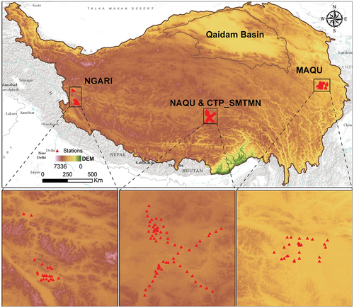
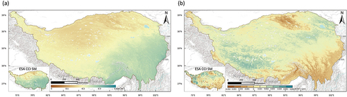
Known as the “Roof of the World,” the Qinghai-Tibet Plateau (QTP) (Figure 1) is the highest and largest plateau in the world with a mean elevation above 4000 m and an area of 2.57 million km² (Wang and Xu 2021). Due to its unique and complex geographical environment, the QTP has diverse climate types, mainly characterizing as temperate and humid in the southeast and arid and cold in the northwest. Therefore, the average precipitation and temperature gradually decreases from the southeast to the northwest (Chen et al. 2015). Moreover, owing to the Indian and Pacific monsoons, summer and autumn account for 73% of the annual precipitation, whereas winter and spring are relatively dry (Qu et al. 2021). Meanwhile, the QTP exerts a crucial role in the Asian atmospheric circulation and even global climate change through thermal and dynamic stress effects (Meng et al. 2018). Hence monitoring the long-term soil moisture on the QTP is pivotal for understanding the response to climate change.

Figure 1. The study area and locations of in-situ measurement networks.

2.2 Datasets

2.2.1 ESA CCI SM product

Aiming to provide a consistent and continuous global SM dataset, the European Space Agency has generated a combined ESA CCI SM product by blending both active and passive SM products (Dorigo et al. 2017; Liu et al. 2012). In this study, the ESA CCI version 07.1 data during 2001–2020 was utilized, which was derived by integrating four active and twelve passive microwave sensors. The model parameterization of the land parameter retrieval model has been improved and an intra-annual bias correction approach was also utilized for harmonization. The temporal span of this daily 0.25° ESA CCI SM product was from 1978 to 2021.

2.2.2 Ancillary datasets

Several auxiliary variables from multisource remote sensing data were utilized in this study (Table 1). Specifically, the daily reflectance data were obtained from three products (e.g. MCD43A4, MOD09GA, MYD09GA) of the Moderate-resolution Imaging Spectroradiometer (MODIS) imageries. The daily daytime land surface temperature (LST) and diurnal temperature difference (LST_Diff) were derived from the MOD11A1, MYD11A1, MOD11A2 and MYD11A2 products. The daily precipitation and evapotranspiration data were obtained from the CHIRPS dataset (Climate Hazards Group InfraRed Precipitation with Station data) and the recently published PML-V2 (China) dataset. The latter was generated using the Penman-Monteith-Leuning water-carbon coupled model (He Shaoyang 2022; He et al. 2022; Zhang et al. 2019). In addition, the soil clay/sand/silt fractions data were from the basic soil property dataset of high-resolution China Soil Information Grids (Liu et al. 2020, 2022; Zhang Ganlin 2021). The elevation data was from the 90 m SRTM (Shuttle Radar Topography Mission), and the slope and aspect were calculated.

Table 1. Lists of the ancillary variables utilized in this study.

Category	Variables	Data set	Spatial resolution	Temporal resolution
Vegetation	Normalized Difference Vegetation Index (NDVI)	MOD09GA& MYD09GA& MCD43A4	1km	Daily
	Enhanced Vegetation Index (EVI)
Energy	Evapotranspiration	PML-V2
	LST	MOD11A, MYD11A1& MOD11A2, MYD11A2
Meteorology	LST_Diff
	Precipitation	CHIRPS	~5km	Daily
Topography	Elevation	HydroSHEDS	90m	Static
	Aspect
	Slope
	Topographic Wetness Index (TWI)
Soil properties	Clay	High-resolution China Soil Information Grids	250m	Static
	Sand
	Silt
Other	Lon/Lat/DOY	—	1km	Static

Meanwhile, 15 SMIs were calculated based on the daily reflectance and LST data, and their potential in downscaling SM was assessed. These indices were mainly categorized into the four types: the SWIR band-based, the NIR band-based, the energy-based and the topography-based indices (Table 2).

Table 2. Lists of the soil moisture-related indices (SMIs) utilized in this study.

Type	Name	Formulation	References
Shortwave Infrared Band based	NMDI	[nir-(swir1-swir2)]/[nir+(swir1-swir2)]	Wang and Qu (2007)
	VSDI	1-[(swir1-blue)+(red-blue)]	Zhang et al. (2013)
	SWCI	(swir1-swir2)/(swir1+swir2)	Hong et al. (2018)
	SIWSI	(swir1-nir)/(swir2+nir)	Fensholt and Sandholt (2003)
Near infrared band based	DDI	[sqrt(red^2+nir^2)]/(1+NDVI)	Qin et al. (2010)
	EVI	2.5*(nir-red)/(nir+6*red-7.5*blue+1)	Huete et al. (1997)
	NDMI	(nir-mir)/(nir+mir)	Gao (1996)
	NDVI	(nir-red)/(nir+red)	Van Deventer et al. (1997)
	SRWI	nir/mir	Zarco-Tejada et al. (2003)
Energy based	ATI	1-albedo/ΔTs	Lu et al. (2014)
	MEI	(1-nir)/Ts	Zhang et al. (2009)
	TVDI	(Ts-Tsmin)/(Tsmax-Tsmin)	Sandholt et al. (2002)
	VCTI	(Tsmax-Ts)/(Tsmax-Tsmin)	Wan et al. (2004)
	VSWI	NDVI/Ts	Carlson et al. (1990)
Topography based	TWI	log10(α/tan β)	Sørensen et al. (2006)

2.2.3 Existing 1 km SM datasets

Two recently released 1 km daily SM datasets over China and one global daily 1 km SM dataset were also selected and evaluated to further justify the added values of generated LHS-SM dataset. Utilizing the AMSR-E/AMSR-2 SM products, Song et al. (2022) generated the 1 km daily surface soil moisture data over China during 2003–2019 (hereafter refers as SMPL dataset). The temperature and vegetation indices were priorly gap-filled and then utilized to obtain the downscaled SM under all-weather conditions based on a semi-physical model. Meanwhile Li et al. (2022a) obtained the 1 km daily soil moisture dataset (hereafter refers as SMCI dataset) in 10 different layers with an interval of 10 cm based on a RF model taking in-situ observations as the target. The SMCI data at the first layer that represents the 10 cm SM was adopted. Han et al. (2023) also generated the global daily 1 km surface SM data (hereafter refers as GSSM dataset) using a physics informed RF model. The SMAP/Sentinel-1 active-passive combined 1 km SM data was not considered due to its extremely large data gaps on the QTP and few valid records for each station (less than 30 records during 2015–2020).

2.2.4 In-situ measurements

The evaluation data were from four in-situ monitoring networks on the QTP (Table 3) and they were obtained from the International Soil Moisture Network (ISMN), which aimed to provide the globally available, harmonized and quality-controlled in-situ soil moisture measurements (Dorigo et al. 2021, 2011). Only good-quality records with 0-10 cm depth (0-5 cm, 5 cm or 10 cm) were utilized and sites having fewer than 30 valid records or having correlation with p value > 0.01 were excluded so as to alleviate the spatial mismatch problem and obtain a relatively fair results (Ma et al. 2019, 2021, 2023).

Table 3. The information of in-situ networks utilized in this study.

Networks	Sites	Climate	Depth used	Frequency	Land use	Data period
CTP_SMTMN	57	Cold humid	5cm, 10cm	hourly	Grassland	2010–2016
MAQU	27	Cold humid	5cm, 10cm	hourly	Grassland	2008–2019
NAQU	11	Cold semiarid	5cm, 10cm	hourly	Grassland	2010–2019
NGARI	23	Cold arid	5cm, 10cm	hourly	Barren land	2010–2019

2.3 Methodology

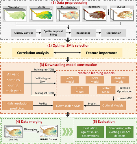
Figure 2 shows the overall framework of generating the daily 1 km LHS-SM data, which consists of five steps: (1) data preprocessing: prepare various remote sensing, in-situ, and model-based data and conduct necessary preprocessing; (2) optimal SMIs selection: evaluate and select the suitable SMI for downscaling; (3) downscaling model construction: construct five machine learning downscaling models for each year; (4) data merging: merge the downscaled surface SM datasets based on a spatiotemporal error; (5) evaluation: evaluate against in-situ measurements and compared with three existing SM datasets.

Figure 2. The overall flowchart of this study.

2.3.1 Data preprocessing

The LST data was further quality controlled and only pixels with good quality (QA = 0 or 1) were retained, inevitably leading to certain degrees of missing data (e.g. the average daily missing percentage after quality control was 37.83% in 2018). Therefore, a gap filling method similar to that proposed by Yang et al. (2019) was applied to obtain the spatiotemporal continuous LST data, which include the following steps: (1) calculate the averaged high-quality eight-day LST from MOD11A2 and MYD11A2 products, and averaged high-quality daily LST from MOD11A1 and MYD11A1 products; (2) temporally interpolate the eight-day LST into daily LST using the harmonic analysis of time series (HANTS) algorithm (Eq. 1); (3) calibrate the interpolated LST using original daily LST with good quality; (4) replace the calibrated LST by original high-quality daily LST when available. The gap-filled LST was validated against original good-quality LST data by artificially masking some pixels as missing areas and showed acceptable accuracy (Appendix A).

(1) $LS{T}_t=\overline{LST}+{\sum }_{i=1}^n{A}_{i}cos\left({\omega }_{i}t-{\phi }_i\right)$(1)

Where $LS{T}_t$ is the reconstructed LST at date t, $\overline{LST}$ is the annual mean LST, $A_i$,${\omega }_i$, and ${\phi }_i$ is the amplitude, phase and frequency of the $i^{th}$ harmonic component, while n is the number of harmonic components (n = 6).

As for surface reflectance data, the daily reflectance values from the three products (i.e. MCD43A4, MOD09GA and MYD09GA) were first averaged and the Savitzky-Golay filtering method was used to fill gaps. The calculated NDVI and EVI data were further filtered and smoothed using the effective HANTS algorithm to reduce noises.

2.3.2 Optimal soil moisture indices selection

Fifteen SMIs were calculated in this study and their potential for downscaling the ESA CCI SM data was evaluated based on correlation coefficients and feature importance. First, the Pearson correlation coefficient between each SMI and ESA CCI SM was calculated and ranked. However, since nonlinear relationship exists between SMIs and SM, and Pearson correlation can only capture linear relationship, the feature importance of each SMI was also obtained through a random forest model taking the SMIs as inputs and the ESA CCI SM as target. The performances of the SMIs were assessed based on these two metrics and the union of each best four SMIs according to R values or feature importance were identified as candidates and indices with high collinearity were excluded.

2.3.3 Downscaling model construction

Firstly, the ancillary variables were projected and resampled to the spatial resolution of ESA CCI SM data using nearest-neighbor interpolation method. Then, for each year, all the available pixels after quality control were extracted, normalized using the Z-score normalization, and randomly divided into the training (70%), validating (20%) and testing (10%) sets. Subsequently, five machine learning models including the ANN, the ResNet, the LSTM, the convolution network (CNN) and the extreme gradient boosting (XGB) were constructed taking the ESA CCI SM as target (Eq. 2).

(2) $S{M}_C=ML\left(X_{1,C},X_{2,C},X_{3,C},X_{4,C}\dots X_{N,C}\right)$(2)

Where the $S{M}_C$ and $X_{1,C}$ represent the coarse-scale SM and ancillary variables, respectively, and ML denotes the constructed downscaling methods.

The structure and hyperparameters of each model were tuned using the Bayesian optimization and the model yielding the lowest mean square error (MSE) was chosen as the optimal model. Subsequently, the high-resolution predictors were fed to the optimal models, resulting in the generation of daily 1 km SM data (Eq. 3).

(3) $S{M}_H=ML\left(X_{1,H},X_{2,H},X_{3,H},X_{4,H}\dots X_{N,H}\right)$(3)

Where the $S{M}_H$ and $X_{1,H}$ represent the high-scale SM and ancillary variables, respectively.

The ANN model that has been widely utilized to represent the complex relationship among variables was adopted in this study to include 4–6 hidden layers with 100–500 neurons. On the other hand, through convolution, the CNN (LeCun et al. 1989) can effectively extract spatial features, thereby outperforming other traditional machine learning methods in terms of spatial patterns. Additionally, the ResNet (He et al. 2016) mitigates the gradient explosion problem by shortcut connections and has been proven to present more feasible spatial patterns and details in downscaled SM (Zhao et al. 2022). By utilizing the time series data, the LSTM (Hochreiter and Schmidhuber 1997) could effectively capture the temporal dynamics of SM and achieve satisfied accuracy in time series prediction. As an ensemble learning method, the XGB shows great capability in tabulate data and its potential in SM downscaling has been fully justified in previous studies (Karthikeyan and Mishra 2021; Zhang et al. 2022).

2.3.4 Data merging

According to Zhou et al. (2021), SM products contain spatiotemporal non-stationary random errors, which might be stationary in one dimension but non-stationary in the other. Therefore, for a specific SM product, the time series at each pixel could be expressed as:

(4) $\mathrm{S}\mathrm{M}=S{M}_{true}+\epsilon =S{M}_{true}+{\epsilon }_t+{\epsilon }_s$(4)

where $S{M}_{true}$ is the true SM value, $\epsilon$ is the zero-mean error of the specific SM product and ${\epsilon }_t$, ${\epsilon }_s$ denote the independent temporal and spatial errors, respectively.

The merged SM data of the N SM products can be obtained from:

(5) $S{M}_m={\sum }_{i=1}^N{w}_{i}S{M}_i={\sum }_{i=1}^N{w}_{i}S{M}_{true}+{\sum }_{i=1}^N{w}_i{\epsilon }_{t,i}+{\sum }_{i=1}^N{w}_i{\epsilon }_{s,i}=S{M}_{true}+{\epsilon }_m$(5)

where

(6) ${\sum }_{i=1}^N{w}_i=1$(6)

(7) ${\epsilon }_m={\sum }_{i=1}^N{w}_i{\epsilon }_{t,i}+{\sum }_{i=1}^N{w}_i{\epsilon }_{s,i}$(7)

Then the variance of error for the merged SM data can be obtained as:

(8) $\mathrm{V}\mathrm{a}\mathrm{r}\left({\epsilon }_m\right)=\mathrm{V}\mathrm{a}\mathrm{r}\left({\sum }_{i=1}^N{w}_i{\epsilon }_{t,i}+{\sum }_{i=1}^N{w}_i{\epsilon }_{s,i}\right)=\mathrm{V}\mathrm{a}\mathrm{r}\left({\sum }_{i=1}^N{w}_i{\epsilon }_{t,i}\right)+\mathrm{V}\mathrm{a}\mathrm{r}\left({\sum }_{i=1}^N{w}_i{\epsilon }_{s,i}\right)=\mathit{w}{\mathit{R}}_{\mathit{t}}{\mathit{w}}^{\mathit{T}}+\mathit{w}{\mathit{R}}_{\mathit{s}}{\mathit{w}}^{\mathit{T}}$(8)

where ${\mathbf{R}}_{\mathbf{t}}$ and ${\mathbf{R}}_{\mathbf{s}}$ are the temporal and spatial error covariance matrixes and $\mathbf{w}$ is the $1\times \mathrm{N}$ weight vector.

The weights can be obtained by minimizing the error variance of merged SM data $\mathrm{V}\mathrm{a}\mathrm{r}\left({\epsilon }_m\right)$ using the Lagrangian algorithm. The ${\mathbf{R}}_{\mathbf{t}}$ and ${\mathbf{R}}_{\mathbf{s}}$ could be estimated using the TCH method (Tavella and Premoli 1994), which has been widely utilized for error estimation and data merging (Liu et al. 2021; Shangguan, Min, and Shi 2023b). Specifically, all the downscaled SM datasets using different machine learning methods on a specific date t across the whole study region were utilized for deriving the spatial error covariance ${\mathbf{R}}_{\mathbf{s}}$ on date t, while the temporal error covariance ${\mathbf{R}}_{\mathbf{t}}$ was estimated for each pixel using the time series of each generated downscaled product.

2.3.5 Evaluation strategies

In order to fairly examine the performance of the LHS-SM data, two evaluation strategies were adopted. Firstly, the generated SM data was evaluated against in-situ measurements. Several evaluation metrics including the correlation coefficient (R), root mean square error (RMSE), the unbiased root mean square error (ubRMSE) and bias (Entekhabi et al. 2010) were calculated as follows:

(9) $\mathrm{R}=\frac{{\sum }_{i=1}^N\left(x_i-\bar{x}\right)\left(y_i-\bar{y}\right)}{\sqrt{{\sum }_{i=1}^N{\left(x_i-\bar{x}\right)}^2{\left(y_i-\bar{y}\right)}^2}}$(9)

(10) $\mathrm{R}\mathrm{M}\mathrm{S}\mathrm{E}=\sqrt{\frac{{\sum }_{i=1}^N{\left(x_i-y_i\right)}^2}{N}}$(10)

(11) $\mathrm{u}\mathrm{b}\mathrm{R}\mathrm{M}\mathrm{S}\mathrm{E}=\sqrt{\frac{{\sum }_{i=1}^N{\left[\left(x_i-\bar{x}\right)-\left(y_i-\bar{y}\right)\right]}^2}{N}}$(11)

(12) $\mathrm{b}\mathrm{i}\mathrm{a}\mathrm{s}=\frac{1}{N}{\sum }_{i=1}^N\left(x_i-y_i\right)$(12)

where $x_i$ and $y_i$ denote the $i$th downscaled SM and in-situ SM observation, and $\bar{x}$ and $\bar{y}$ represent the mean values of the downscaled SM and in-situ SM observation, respectively.

Secondly, the performance of LHS-SM data was compared with three existing 1 km SM datasets (Section 2.3.3) to further demonstrate its potential values. In-situ values were averaged on a daily scale before evaluation and station values within the same satellite grid were averaged to alleviate spatial mismatching issue (Li et al. 2022, 2022; Ma et al. 2019, 2021). The 10 cm observations were utilized for the SMCI product, while the LHS-SM and SMPL products were evaluated against the 5 cm (0-5 cm or 5 cm) measurements.

3 Results

3.1 Selection of soil moisture indices

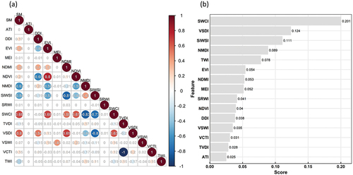
The correlation coefficients between SMIs and ESA CCI SM, as well as the feature importance of RF model are shown in Figure 3. Six of the fifteen indices presented acceptable correlations with SM (absolute value of R > 0.3 and p-value <0.01). Among them, the SWCI had the highest correlation with the R value of 0.66, followed by the NMDI and VSDI indices. Conversely, the energy-based ATI and MEI exhibited the weakest correlations. The feature importance revealed similar results, indicating the SWCI, VSDI and SIWSI as the three most influential features, while the impact of ATI was relatively inconsequential. The TWI also showed certain influence on SM. In general, such results implied the high sensitivity and great characterization capability of SWIR band to SM variation, which was consistent with previous studies (Wei et al. 2019; Zhang et al. 2022). Even though the LST was found to have a strong relationship with SM in previous researches (Senanayake et al. 2021; Wei et al. 2019), the derived indices such as the ATI, MEI, TVDI showed relatively weaker performances compared to those based on SWIR (e.g. SWCI, VSDI, NMDI et.al.) and NIR (e.g. DDI, NDMI, SRWI, NDVI) indices. According to both the correlation and feature importance analysis, the SWCI, VSDI, SIWSI and NMDI were identified as the best four indices but the NMDI was further excluded due to its strong collinearity with SWCI. In addition, due to the saturation of NDVI over dense vegetated regions, both the NDVI and EVI were chosen to fully represent the vegetation factor despite their high correlation, and the TWI was also selected as the topography impact.

Figure 3. The (a) correlation of soil moisture-related indices (SMIs) with SM and (b) the feature importance of each SMI.

3.2 Comparison with ESA CCI SM product

3.2.1 Evaluation against in-situ measurements

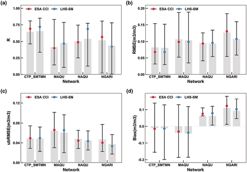
The evaluation results of both the ESA CCI and LHS-SM soil moisture products against ground observations at station scale are presented in Figure 4. Overall the mean values of the network-averaged R, ubRMSE, RMSE and bias metrics for LHS-SM dataset were 0.52, 0.047 m³/m³, 0.096 m³/m³ and 0.025 m³/m³, respectively and were 0.51, 0.052 m³/m³, 0.102 m³/m³ and 0.030 m³/m³ for the ESA CCI SM data. Compared with original ESA CCI SM data, certain improvement was achieved for the generated product with regards of R and ubRMSE. Specifically, for the R value, the LHS-SM showed higher correlation than ESA CCI both in CTP_SMTMN, MAQU and NAQU networks with mean R scores improved by 0.02 to 0.05. However, the mean R value for the BTCH SM data in NGARI network was lower than that of ESA CCI SM data. As for the ubRMSE metric, the LHS-SM data presented lower ubRMSE values than the ESA CCI SM data in all four networks. The ubRMSE for the generated SM ranged between 0.038 and 0.060 m³/m³, and between 0.047–0.64 m³/m³ for the ESA CCI product. As for the RMSE score, the mean value of LHS-SM and ESA CCI SM ranged from 0.080–0.107 m³/m³ and 0.081–0.127 m³/m³, respectively. Nevertheless, the LHS-SM data showed slightly larger bias than the ESA CCI SM data both in CTP_SMTMN, MAQU and NAQU networks and relatively smaller bias in NGARI network with a reduction of 0.017 m³/m³.

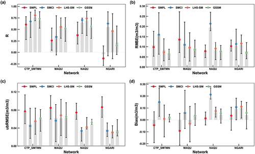
Figure 4. Evaluation metrics of both ESA CCI and LHS-SM data for each network: (a) R, (b) RMSE, (c) ubRMSE and (d) bias. The grey bar represents the mean values of evaluation metrics.

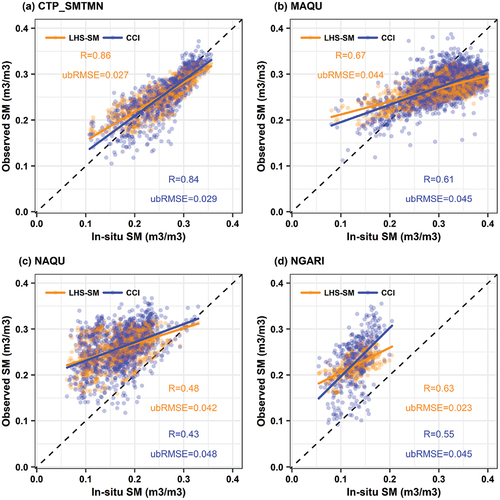
Figure 5 shows the scatter plot of LHS-SM and ESA CCI SM against in-situ measurements at network scale (values within the same network were averaged on a daily scale). Both the LHS-SM and ESA CCI SM data performed the best in CTP_SMTMN network, followed by the MAQU and NGARI networks. While the NAQU network showed the worst accuracy. Compared with the ESA CCI SM data, the generated SM data exhibited various degrees of improvements, indicating that the LHS-SM data could capture the evolution of surface soil moisture more accurately. The NGARI network presented the largest improvement with correlation increased by 0.08 and ubRMSE reduced by 0.023 m³/m³. While the R and ubRMSE scores for the other three networks were improved by 0.03–0.06 and 0.001–0.006 m³/m³, respectively.

Figure 5. The scatter plots of ESA CCI and LHS-SM data against in-situ measurements for (a) CTP_SMTMN, (b) MAQU, (c) NAQU and (d) NGARI network.

3.2.2 Advantages of LHS-SM data over ESA CCI SM

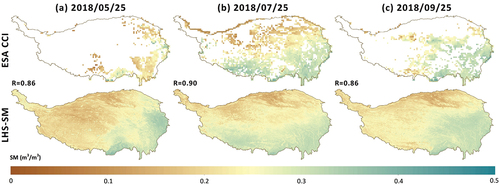
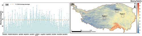
The ESA CCI suffered from data gaps on the QTP with an average daily missing percentage of 81.59% during 2001–2020 (Figure 6). Spatially, the northwestern of the QTP was confronted with extremely large gaps with the missing rate basically above 85%, while the eastern regions had relatively smaller missing rates ranging from 10% to 80%. While the generated LHS-SM, in contrast, was spatiotemporally seamless due to the utilization of gap-filled auxiliary variables. In addition, the spatial distribution of ESA CCI SM and LHS-SM data on three selected dates are presented in Figure 7. The LHS-SM data can well preserve the patterns of ESA CCI SM with relatively high correlation and show reasonable continuous SM values in data missing areas. Given the evaluation results in Section 3.2.1, it could be concluded that the LHS-SM data had obvious advantages over the ESA CCI SM data both in spatiotemporal continuity and spatial resolution while maintaining high accuracy.

Figure 6. The data missing condition of the ESA CCI SM data during 2001–2020: (a) the daily data missing percentage and (b) the pixel-wise data missing rate.

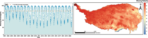
Figure 7. The comparison of the ESA CCI SM and LHS-SM data on three selected dates: (a) 25th May 2018, (b) 25th July 2018 and (c) 25th September 2018.

3.3 Comparison with existing soil moisture products

3.3.1 Evaluated against in-situ measurements

The evaluation and comparison results of the SMPL, SMCI, LHS-SM and GSSM SM data are shown in Figure 8. Overall, the LHS-SM data had the best performance followed by the SMCI, GSSM and the SMPL data. The averaged R/ubRMSE values were 0.62/0.047 m³/m³, 0.54/0.44 m³/m³, 0.49/0.051 m³/m³ and 0.29/0.078 m³/m³ for the LHS-SM, SMCI, GSSM and SMPL data, respectively. Specifically, the SMCI SM data had relatively high correlation (R > 0.5) expect for the MAQU network and the lowest ubRMSE scores in CTP_SMTMN and NAQU networks. However, it showed inferior performance in terms of RMSE and bias with mean scores ranging between 0.10–0.21 m³/m³ and 0.067–0.202 m³/m³ among networks. Similarly, the GSSM data exhibited relatively high correlation in the CTP_SMTMN, NAQU and MAQU networks and low ubRMSE scores (<0.05 m³/m³) in the NAQU and NGARI networks. Meanwhile, it also owned the lowest RMSE values in each network and the bias scores were between 0.17 m³/m³ and 0.042 m³/m³. The SMPL SM product, on the contrary, exhibited much inferior accuracy with the lowest correlation coefficient and highest ubRMSE value in each network. The mean R value was even negative in NGARI network. Besides, there existed certain underestimation for the SMPL product, especially in MAQU network with a mean bias value of −0.095 m³/m³. As for the LHS-SM product, it outperformed the SMCI, GSSM and SMPL products with significantly higher correlation (p-value <0.01) and the lower RMSE and bias scores. The ubRMSE score was also significantly lower (p-value <0.01) than the GSSM and SMPL data with mean values ranging between 0.033 and 0.062 m³/m³.

Figure 8. Evaluation metrics of SMPL, SMCI, LHS-SM and GSSM SM data for each network: (a) R, (b) RMSE, (c) ubRMSE and (d) bias. The grey bar represents the mean values of evaluation metrics.

3.3.2 Spatiotemporal comparison

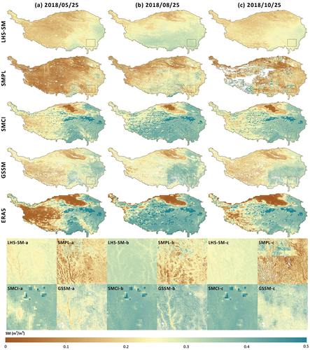
The spatial distribution of the LHS-SM, SMPL, SMCI, GSSM, and ERA5-Land SM data on three selected dates are displayed in Figure 9. Even though all the SM products exhibited generally similar spatial patterns, the SMCI data, compared with other three SM datasets, was obviously overestimated in most regions with SM values greater than 0.4 m³/m³. Moreover, the distribution of SMCI SM product was extremely similar to the ERA5-Land SM data with relatively dry moisture in the Qaidam Basin and high SM values in the central areas. Such similarity might be attributed to the fact that ERA5-Land SM was utilized as an ancillary variable for SMCI and its feature importance was much higher than other predictors (Li et al. 2022). Besides, it was blurred to a certain extent and the detailed SM information was lost in some regions (zoomed in plots for SMCI dataset). The GSSM data, however, showed an unnatural moisture transition in horizontal direction in the central regions, which was not observed in other three datasets. In addition, it presented relatively dry moisture condition in the bottom central regions (e.g. the Medog and Cona County), but the SM values in these regions were quite high for the LHS-SM, SMPL and SMCI data. The variation among different dates also obviously differed from the other three SM products. As for the SMPL product, it still showed certain degrees of data gaps with an average missing rate of 25.45% even after masking out the water bodies, permanent soil and ice areas. Meanwhile, it displayed discontinuous and abnormal distribution in cold regions and unreasonably high value, and obvious grid effect could be observed (zoomed in plots for SMPL dataset).

Figure 9. The spatial distribution of the LHS-SM, SMPL, SMCI, GSSM and ERA5-land SM data on (a) 25th May 2018, (b) 25th August 2018 and (c) 25th October 2018. Insets show a zoomed-in place located in the southeastern of the QTP.

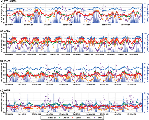
The temporal series of in-situ values and the LHS-SM, GSSM, SMCI and SMPL SM data for each network are also presented in Figure 10. All the SM products could well capture the SM dynamics and corresponded well to precipitation variations. The LHS-SM data was in better line with the ground truth than the other three SM datasets in all networks with higher correlation and lower error, especially in the CTP_SMTMN network (R = 0.90). The SMCI product, however, showed various degrees of overestimation in CTP_SMTMN, MAQU and NAQU networks and such overestimation was alleviated in NGARI network. The performance of GSSM data was relatively inferior than the SMCI data in the CTP_SMTMN, MAQU and NAQU networks (R value between 0.47–0.86), but was quite poor in NGARI network with R values of only 0.048. As for the SMPL dataset, it accurately estimated SM with acceptable correlations in summer but displayed significantly unreasonable fluctuations in winter. At the same time, it showed the lowest correlation in each network and even had a R value of −0.23 in NGARI network. Data gaps could also be observed in winders. This might be associated with the adopted downscaling algorithms. The SMPL dataset mainly depended on the semi-physical empirical relationship between SM and LST. The downscaled SM was more prone to the abnormal information of LST data and had unreasonable distributions and data gaps in cold regions and seasons (Figure 9).

Figure 10. The time series of soil moisture from the in-situ observation (orange dot), LHS-SM (green dot), SMPL (purple dot), GSSM (red dot) and SMCI (blue dot) SM data, and precipitation (blue bar) for (a) CTP_SMTMN, (b) MAQU, (c) NAQU and (d) NGARI network.

4 Discussion

4.1 Feasibility of soil moisture-related indices in downscaling

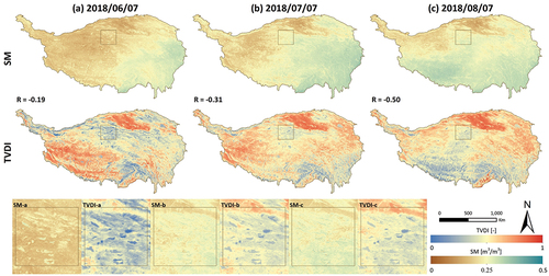
The feasibility of several SMIs was evaluated in this study and results indicated that the SWIR-based indices such as the SWCI, NMDI, VSDI yielded the highest performance due to the strong physical connection of SWIR band to moisture dynamics. Such finding was also confirmed by previous studies and the SWIR band have been widely utilized to estimate SM (Sadeghi, Jones, and Philpot 2015; Yue et al. 2019; Zhang et al. 2022). Since the NIR band was sensitive to both moisture and vegetation, the derived indices (DDI, NDMI, SRWI, NDVI) showed relative weaker relationship with SM. As another key factor connected to SM, the surface temperature change is inversely related to SM according to the thermal inertia theory (Sabaghy et al. 2018; Senanayake et al. 2021). Therefore, the LST-VI feature space has been exploited to downscale SM products (Merlin et al. 2012; Peng, Niesel, and Loew 2015) and the derived indices (TVDI, VTCI, VSWI) have been successfully applied to obtain fine scale SM data (Meng et al. 2021). Nevertheless, such method usually requires the underlying surface to be uniform and covered with enough vegetation coverage conditions to ensure the robustness of constructed dry and wet edge equations. In addition, these indices are not temporally comparable and unsuitable for directly estimating SM time series, since they are obtained under different atmospheric conditions, which greatly affect the feature space. Their downscaling potentials were also limited to a certain extent on the QTP due to its complex geography and large spatial heterogeneity of land surface. For example, even though the TVDI is theoretically inversely related with SM, their relationship varied over time and was much stronger in summer (Figure 11). Besides such relationship showed strongly spatial heterogenicity and the TVDI could better reflect SM distribution in the southwestern regions than in the eastern areas, where high moisture coexisted with high TVDI value. The TVDI presented less sensitivity to SM in densely vegetated regions. The relatively poor performance of SMPL SM data in cold regions (NGARI network) also indicated the limitation of the LST-VI feature space-based downscaling method (Section 3.3).

Figure 11. The spatial maps of LHS-SM data and TVDI on three selected days: (a) 7th June 2018, (b) 7th July 2018 and (c) 7th August 2018.

4.2 Spatiotemporal patterns of soil moisture

The mean SM map and linear trend of annual average LHS-SM and ESA CCI SM data during 2001–2020 are shown in Figure 12. The LHS-SM data presented similar spatiotemporal patterns with the ESA CCI SM but had lower moisture values in the southwestern regions. Such behavior was reasonable considering the relatively larger bias of ESA CCI SM than the LHS-SM data (Section 3.2.1). The distribution of SM on the QTP was mainly influenced by the climate and topography (Shangguan, Min, and Shi 2023b; Zhang et al. 2022), and exhibited a gradually drying pattern from east to west and from south to north. Quite dry statue was observed in the Qaidam Basin, while the southeastern regions were relatively humid. However, the annual trend of SM showed a different pattern. The southwestern part of the plateau and the area around Qinghai Lake in the northeast showed a gradually wetting trend, while SM in the Qaidam Basin and the southeastern regions became increasingly dry. Besides, it could be concluded that there was a strong spatial heterogeneity in the SM dynamic pattern on the QTP. The “dry gets drier” scheme was mainly occurred in the Qaidam Basin regions, whereas the “wet gets wetter” pattern was not observed. On the contrary, the southeastern regions exhibited a “wet gets drier” trend. While the northeast and southwest of the QTP presented a “dry gets wetter” scheme and such change pattern was reasonable since the QTP had experienced an overall warming and humidification in the past decades due to global warming.

Figure 12. The spatial pattern of (a) annual mean LMS-SM and (b) linear trend of annual mean LHS-SM data during 2001–2020. Water bodies, snow and ice were excluded.

4.3 Limitations and prospects

Despite the high accuracy of the obtained LHS-SM dataset, there still exist certain limitations and drawbacks. Firstly, Although the LST data gaps due to cloud containment was filled with an acceptable accuracy (Appendix A), it should be noted that the reconstructed LST was only a proxy of theoretical clear-sky LST rather than actual LST under cloud conditions, since the information to estimate the cloudy LST was from the spatiotemporal neighboring clear-sky pixels (Song et al. 2022). Therefore, certain degrees of systematic bias exist in the reconstructed LST and would further affect the accuracy of downscaled SM because of the strong connection between LST and SM according to the thermal inertia theory. More accurate and effective gap-filling methods should be applied to generate the continuous LST data under all-weather conditions (Long et al. 2020; Zeng et al. 2018).

In addition, there are two main processes for obtaining the fine-scale SM data: the prediction of SM over data missing areas and disaggregation from coarse SM pixels. Leng et al. (2023) investigated the performances of two downscaling schemes and found that the disaggregation-first scheme outperformed the prediction-first scheme possibly due to the more valid training data in the former method. In this study, however, the downscaling models were constructed at coarse scale and directly applied for fine-scale SM prediction. Their performances were thus influenced by the data missing condition of ESA CCI SM product to a certain extent. Besides, the scale effect during aggregation and model application processes also hampered the accuracy of downscaled SM.

Frozen surfaces and snow cover were masked out in the ESA CCI SM data using brightness temperature data in three frequencies (van der Vliet et al. 2020). The constructed downscaling models, thus, had inferior capability in characterizing the relationship between SM and ancillary variables during frozen seasons and yielded higher SM values than observations due to less valid samples in frozen seasons (Figure 10). However, it has been well acknowledged that liquid water and ice coexist in soil under subfreezing temperature and a small portion of bound water cannot undergo phase transition (He and Dyck 2013; Wu et al. 2022). Therefore, the downscaled SM data in frozen seasons was retained as a rough reference despite its relatively large uncertainty, but should be used with caution. Certain calibration methods should be exploited to obtain accuracy SM values in frozen seasons in future study.

5 Conclusions

The long-term, high-accuracy and seamless soil moisture dataset (LHS-SM) over the QTP during 2001–2020 was generated in this study using a two-step downscaling method. The feasibility of 15 SMIs and the performance of obtained LHS-SM data were fully assessed and the main conclusions were as below:

1. The potentials of several SMIs in downscaling SM were assessed and the SWCI, VSDI, SIWSI were identified as the optimal indices. The SWIR derived indices presented better performance due to the strong sensitivity of SWIR band to moisture, while the LST-VI space-based indices showed certain limitation on the QTP.

2. Compared with ESA CCI SM product, certain improvement was achieved by the LHS-SM dataset both in terms of correlation and error. The mean R and ubRMSE values for the LHS-SM data were 0.52, 0.047 m³/m³ and were 0.51, 0.052 m³/m³ for the ESA CCI SM data. In addition, comparison with existing 1 km SM datasets revealed that the LHS-SM data showed the best performance over the QTP with the significantly higher correlation and relatively low ubRMSE, while previous datasets either lost some spatial details or had certain data gaps and unreasonable distribution on the QTP.

3. The annual mean SM on the QTP during 2001-2020 gradually decreased from the southeast to northwest and the SM dynamics exhibited strong spatial heterogeneity. The “dry gets drier” pattern was observed in the Qaidam Basin, while the southeast of the plateau presented a “wet gets drier” trend. Due to global warming, the southwestern and northeastern regions showed a “dry gets wetter” scheme.

In conclusion, the obtained LHS-SM dataset owned its values by compensating the limitations of existing high-resolution SM products over the QTP and could be widely utilized in many regional applications.

Author contributions

Yulin Shangguan: Conceptualization, Data curation, Formal analysis, Methodology, Validation, Visualization, Writing original draft. Xiaoxiao Min: Conceptualization, Data curation, Methodology, Review and editing. Nan Wang: Reviewing and editing. Cheng Tong: Conceptualization, Reviewing and editing. Zhou Shi: Conceptualization, Supervision, Reviewing and editing.

Acknowledgments

The authors are grateful to all the data providers and the anonymous reviewers for their detailed and constructive comments.

Disclosure statement

No potential conflict of interest was reported by the author(s).

Data availability statement

The MODIS reflectance and land surface temperature data, CHIRPS and DEM data are available through Google Earth Engine (https://developers.google.com/earth-engine/). The soil properties data are available through https://poles.tpdc.ac.cn/en/data. The SMCI, SMPL can be freely downloaded from https://www.tpdc.ac.cn. The GSSM SM data is available from https://doi.org/10.6084/m9.fgshare.21806457.v1. The generated LHS-SM dataset can be freely assessed through https://doi.org/10.5281/zenodo.7619545 (part 1, 2001–2010) and https://doi.org/10.5281/zenodo.8016135 (part 2, 2011–2020). All the codes including training model and predicting are available through GitHub (https://github.com/Mew-YL/BTCH).

Additional information

Funding

This work was supported by the National Natural Science Foundation of China [41930754]; the Fundamental Research Funds for the Central Universities [226-2023-00096; 226-2023-00112].

Appendix A:

Validation of gap-filled LST data

The validation results of gap-filled LST data against original LST in 2018 were presented here to justify the feasibility of LST gap filling method. The missing percentage of averaged daily LST data from both MOD11A1 and MYD11A1 products after quality control was showed in Figure A1. Certain data gaps existed in the daily LST data with an average missing percentage of 37.83%. From the perspective of spatial pattern, the eastern of the QTP had larger missing rate than the western regions and the Linzhi city in the southeastern QTP severely suffered from cloud containment with a mean missing rate above 80%.

Figure A1. The data missing condition of the daily LST data in 2018: (a) the daily data missing percentage and (b) the pixel-wise data missing rate.

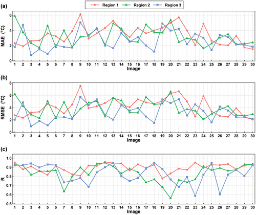
In order to examine the performance of gap filling method, three regions with different missing percentages were selected and 30 dates were chosen when all the three regions had a missing rate less than 15%. Then for each region, an area was masked out to simulate the missing pixels and reconstructed using the gap filling method. The correlation coefficient (R), root mean square error (RMSE) and mean absolute error (MAE) metrics against original pixels were calculated.

Figure A2. The scatter density plots of reconstructed LST against original LST in (a) region 1, (b) region 2 and (c) region 3.

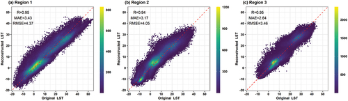
Overall the gap-filled LST had an acceptable accuracy against original LST with R values above 0.94, RMSE values ranging between 3.46-4.37°C, and MAE values ranging between 2.64-3.43°C (Figure A2). Spatially, the adopted gap filling method could well reconstruct LST data gaps with satisfying performance but showed slightly lower values than the real LST (Figure A3). In addition, the accuracy varied over time and region 1 outperformed other regions in terms of R metric with a mean R score of 0.89 but had relatively larger mean MAE and RMSE values than other two regions (Figure A4).

Figure A3. The (a) original good-quality LST, (b) simulated missing LST and (c) gap-filled LST on 2th April, 2018 over three selected regions and the pixel-wise (d) MAE, (e) RMSE and (f) R values for the zoomed-in simulated missing regions.

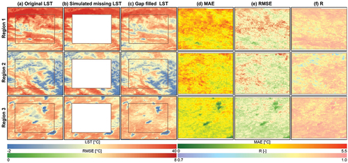
Figure A4. The (a) MAE, (b) RMSE and (c) R metric of reconstructed LST against original LST over three regions on 30 selected dates in 2018.

References

- Abowarda, A. S., L. Bai, C. Zhang, D. Long, X. Li, Q. Huang, and Z. Sun. 2021. “Generating Surface Soil Moisture at 30 M Spatial Resolution Using Both Data Fusion and Machine Learning Toward Better Water Resources Management at the Field Scale.” Remote Sensing of Environment 255:112301. https://doi.org/10.1016/j.rse.2021.112301
- Carlson, T. N., E. M. Perry, and T. J. Schmugge. 1990. “Remote Estimation of Soil Moisture Availability and Fractional Vegetation Cover for Agricultural Fields.” Agricultural and Forest Meteorology 52:45–23. https://doi.org/10.1016/0168-1923(90)90100-K
- Chawla, I., L. Karthikeyan, and A. K. Mishra. 2020. “A Review of Remote Sensing Applications for Water Security: Quantity, Quality, and Extremes.” Canadian Journal of Fisheries and Aquatic Sciences 585:124826. https://doi.org/10.1016/j.jhydrol.2020.124826
- Chen, X., S. An, D. W. Inouye, and M. D. Schwartz. 2015. “Temperature and Snowfall Trigger Alpine Vegetation Green-Up on the World’s Roof.” Global Change Biology 21:3635–3646. https://doi.org/10.1111/gcb.12954 10
- Chen, C.-F., N.-T. Son, L.-Y. Chang, and C.-C. Chen. 2011. “Monitoring of Soil Moisture Variability in Relation to Rice Cropping Systems in the Vietnamese Mekong Delta Using MODIS Data.” Applied Geography 31:463–475. https://doi.org/10.1016/j.apgeog.2010.10.002
- Das, N. N., D. Entekhabi, E. G. Njoku, J. J. C. Shi, J. T. Johnson, and A. Colliander. 2014. “Tests of the SMAP Combined Radar and Radiometer Algorithm Using Airborne Field Campaign Observations and Simulated Data.” IEEE Transactions on Geoscience & Remote Sensing 52 (4): 2018–2028. https://doi.org/10.1109/TGRS.2013.2257605.
- Dorigo, W., I. Himmelbauer, D. Aberer, L. Schremmer, I. Petrakovic, L. Zappa, W. Preimesberger, et al. 2021. “The International Soil Moisture Network: Serving Earth System Science for Over a Decade, Hydrol.” Earth System Science 25 (11): 5749-5804, 10.5194/hess-25-5749–2021. https://doi.org/10.5194/hess-25-5749-2021.
- Dorigo, W., W. Wagner, C. Albergel, F. Albrecht, G. Balsamo, L. Brocca, D. Chung, et al. 2017. “ESA CCI Soil Moisture for Improved Earth System Understanding: State-Of-The Art and Future Directions.” Remote Sensing of Environment 203:185–215. https://doi.org/10.1016/j.rse.2017.07.001
- Dorigo, W. A., W. Wagner, R. Hohensinn, S. Hahn, C. Paulik, A. Xaver, A. Gruber, et al. 2011. “The International Soil Moisture Network: A Data Hosting Facility for Global in situ Soil Moisture Measurements, Hydrol.” Earth System Science 15 (5): 1675-1698, 10.5194/hess-15-1675–2011. https://doi.org/10.5194/hess-15-1675-2011.
- Entekhabi, D., E. G. Njoku, P. E. O. Neill, K. H. Kellogg, W. T. Crow, W. N. Edelstein, J. K. Entin, et al. 2010. The Soil Moisture Active Passive (SMAP) Mission, Proceedings of the IEEE 98 (5): 704–716. https://doi.org/10.1109/JPROC.2010.2043918
- Fensholt, R., and I. Sandholt. 2003. “Derivation of a Shortwave Infrared Water Stress Index from MODIS Near- and Shortwave Infrared Data in a Semiarid Environment.” Remote Sensing of Environment 87:111–121. https://doi.org/10.1016/j.rse.2003.07.002
- Gao, B.-C. 1996. “NDWI—A Normalized Difference Water Index for Remote Sensing of Vegetation Liquid Water from Space.” Remote Sensing of Environment 58:257–266. https://doi.org/10.1016/S0034-4257(96)00067-3
- Guillod, B. P., B. Orlowsky, D. G. Miralles, A. J. Teuling, and S. I. Seneviratne. 2015. “Reconciling Spatial and Temporal Soil Moisture Effects on Afternoon Rainfall.” Nature Communications 6:6443. https://doi.org/10.1038/ncomms7443
- Han, Q., Y. Zeng, L. Zhang, C. Wang, E. Prikaziuk, Z. Niu, and B. Su. 2023. “Global Long Term Daily 1 km Surface Soil Moisture Dataset with Physics Informed Machine Learning.” Scientific Data 10 (1): 10.1038/s41597-023-02011–7. https://doi.org/10.1038/s41597-023-02011-7.
- He, H., and M. Dyck. 2013. “Application of Multiphase Dielectric Mixing Models for Understanding the Effective Dielectric Permittivity of Frozen Soils.” Vadose Zone Journal 12 (1): 1–22. https://doi.org/10.2136/vzj2012.0060
- He Shaoyang, Z. Y. 2022. “Evapotranspiration and Gross Primary Production dataset(2000.02.26-2020.12.31), National Tibetan Plateau/Third Pole Environment Data Center [Dataset].” PML-V2(china). https://doi.org/10.11888/Terre.tpdc.272389.
- He, S., Y. Zhang, N. Ma, J. Tian, D. Kong, and C. Liu. 2022. “A Daily and 500m Coupled Evapotranspiration and Gross Primary Production Product Across China During 2000–2020.” Earth System Science Data 14 (12): 5463-5488, 10.5194/essd-14-5463–2022. https://doi.org/10.5194/essd-14-5463-2022.
- He, K., X. Zhang, S. Ren, and J. Sun: Deep Residual Learning for Image Recognition, 2016 IEEE Conference on Computer Vision and Pattern Recognition (CVPR), 27-30 June 2016, 770–778, https://doi.org/10.1109/CVPR.2016.90
- Hochreiter, S., and J. Schmidhuber. 1997. “Long Short-Term Memory.” Neural Computation 9:1735–1780. https://doi.org/10.1162/neco.1997.9.8.1735.
- Hong, Z., W. Zhang, C. Yu, D. Zhang, L. Li, and L. Meng. 2018. “SWCTI: Surface Water Content Temperature Index for Assessment of Surface Soil Moisture Status, 10.3390/s18092875.” Sensors 18 (9): 2875. https://doi.org/10.3390/s18092875.
- Huete, A. R., H. Q. Liu, K. Batchily, and W. van Leeuwen. 1997. “A Comparison of Vegetation Indices Over a Global Set of TM Images for EOS-MODIS.” Remote Sensing of Environment 59 (3): 440–451. https://doi.org/10.1016/S0034-4257(96)00112-5.
- Jin, Y., Y. Ge, Y. Liu, Y. Chen, H. Zhang, and G. B. Heuvelink. 2021. “M.: A Machine Learning-Based Geostatistical Downscaling Method for Coarse-Resolution Soil Moisture Products.” IEEE Journal of Selected Topics in Applied Earth Observations & Remote Sensing 14:1025–1037. https://doi.org/10.1109/JSTARS.2020.3035386.
- Karamouz, M., R. S. Alipour, M. Roohinia, and M. Fereshtehpour. 2022. “A Remote Sensing Driven Soil Moisture Estimator: Uncertain Downscaling with Geostatistically Based Use of Ancillary Data.” Water Resources Research 58:e2022WR031946. https://doi.org/10.1029/2022WR031946.
- Karthikeyan, L., and A. K. Mishra. 2021. “Multi-Layer High-Resolution Soil Moisture Estimation Using Machine Learning Over the United States.” Remote Sensing of Environment 266:112706. https://doi.org/10.1016/j.rse.2021.112706.
- Koster, R. D., P. A. Dirmeyer, Z. Guo, G. Bonan, E. Chan, P. Cox, C. T. Gordon, et al. 2004. “Regions of Strong Coupling Between Soil Moisture and Precipitation.” Science 305:1138–1140. https://doi.org/10.1126/science.1100217.
- LeCun, Y., B. Boser, J. S. Denker, D. Henderson, R. E. Howard, W. Hubbard, and L. D. Jackel. 1989. “Backpropagation Applied to Handwritten Zip Code Recognition.” Neural Computation 1:541–551. https://doi.org/10.1162/neco.1989.1.4.541.
- Leng, P., Z. Yang, Q.-Y. Yan, G.-F. Shang, X. Zhang, X.-J. Han, and Z.-L. Li. 2023. “A Framework for Estimating All-Weather Fine Resolution Soil Moisture from the Integration of Physics-Based and Machine Learning-Based Algorithms.” Computers and Electronics in Agriculture 206:107673. https://doi.org/10.1016/j.compag.2023.107673.
- Li, Q., G. Shi, W. Shangguan, V. Nourani, J. Li, L. Li, F. Huang, et al. 2022. “A 1km Daily Soil Moisture Dataset Over China Using in situ Measurement and Machine Learning.” Earth System Science Data 14 (12): 5267–5286. https://doi.org/10.5194/essd-14-5267-2022.
- Liu, J., L. Chai, J. Dong, D. Zheng, J. P. Wigneron, S. Liu, J. Zhou, et al. 2021. “Uncertainty Analysis of Eleven Multisource Soil Moisture Products in the Third Pole Environment Based on the Three-Corned Hat Method.” Remote Sensing of Environment 255:112225. https://doi.org/10.1016/j.rse.2020.112225.
- Liu, Y. Y., W. A. Dorigo, R. M. Parinussa, R. A. M. de Jeu, W. Wagner, M. F. McCabe, J. P. Evans, and A. I. J. M. van Dijk. 2012. “Trend-Preserving Blending of Passive and Active Microwave Soil Moisture Retrievals.” Remote Sensing of Environment 123:280–297. https://doi.org/10.1016/j.rse.2012.03.014.
- Liu, F., H. Wu, Y. Zhao, D. Li, J.-L. Yang, X. Song, Z. Shi, A. X. Zhu, and G.-L. Zhang. 2022. “Mapping High Resolution National Soil Information Grids of China.” Science Bulletin 67:328–340. https://doi.org/10.1016/j.scib.2021.10.013.
- Liu, F., G.-L. Zhang, X. Song, D. Li, Y. Zhao, J. Yang, H. Wu, and F. Yang. 2020. “High-Resolution and Three-Dimensional Mapping of Soil Texture of China.” Geoderma 361:114061. https://doi.org/10.1016/j.geoderma.2019.114061.
- Li, X., J.-P. Wigneron, L. Fan, F. Frappart, S. H. Yueh, A. Colliander, A. Ebtehaj, et al. 2022. “A New SMAP Soil Moisture and Vegetation Optical Depth Product (SMAP-IB): Algorithm, Assessment and Inter-Comparison.” Remote Sensing of Environment 271:112921. https://doi.org/10.1016/j.rse.2022.112921.
- Li, X., J.-P. Wigneron, F. Frappart, G. D. Lannoy, L. Fan, T. Zhao, L. Gao, et al. 2022c. “The First Global Soil Moisture and Vegetation Optical Depth Product Retrieved from Fused SMOS and SMAP L-Band Observations.” Remote Sensing of Environment 282:113272. 10.1016/j.rse.2022.113272.
- Long, D., L. Bai, L. Yan, C. Zhang, W. Yang, H. Lei, J. Quan, X. Meng, and C. Shi. 2019. “Generation of Spatially Complete and Daily Continuous Surface Soil Moisture of High Spatial Resolution.” Remote Sensing of Environment 233:111364. https://doi.org/10.1016/j.rse.2019.111364.
- Long, D., L. Yan, L. Bai, C. Zhang, X. Li, H. Lei, H. Yang, et al. 2020. “Generation of MODIS-Like Land Surface Temperatures Under All-Weather Conditions Based on a Data Fusion Approach.” Remote Sensing of Environment 246:111863. https://doi.org/10.1016/j.rse.2020.111863.
- Lu, L., G.-P. Luo, and J.-Y. Wang. 2014. “Development of an ATI-NDVI Method for Estimation of Soil Moisture from MODIS Data.” International Journal of Remote Sensing 35:3797–3815. https://doi.org/10.1080/01431161.2014.919677.
- Ma, H., X. Li, J. Zeng, X. Zhang, J. Dong, N. Chen, L. Fan, et al. 2023. “An Assessment of L-Band Surface Soil Moisture Products from SMOS and SMAP in the Tropical Areas.” Remote Sensing of Environment 284:113344. https://doi.org/10.1016/j.rse.2022.113344.
- Ma, H., J. Zeng, N. Chen, X. Zhang, M. H. Cosh, and W. Wang. 2019. “Satellite Surface Soil Moisture from SMAP, SMOS, AMSR2 and ESA CCI: A Comprehensive Assessment Using Global Ground-Based Observations.” Remote Sensing of Environment 231:111215. https://doi.org/10.1016/j.rse.2019.111215.
- Ma, H., J. Zeng, X. Zhang, P. Fu, D. Zheng, J.-P. Wigneron, N. Chen, and D. Niyogi. 2021. “Evaluation of Six Satellite- and Model-Based Surface Soil Temperature Datasets Using Global Ground-Based Observations.” Remote Sensing of Environment 264:112605. https://doi.org/10.1016/j.rse.2021.112605.
- Meng, X., R. Li, L. Luan, S. Lyu, T. Zhang, Y. Ao, B. Han, L. Zhao, and Y. Ma. 2018. “Detecting Hydrological Consistency Between Soil Moisture and Precipitation and Changes of Soil Moisture in Summer Over the Tibetan Plateau.” Climate Dynamics 51 (11–12): 4157-4168, 10.1007/s00382-017-3646–5. https://doi.org/10.1007/s00382-017-3646-5.
- Meng, X., K. Mao, F. Meng, J. Shi, J. Zeng, X. Shen, Y. Cui, L. Jiang, and Z. Guo. 2021. “A fine-resolution soil moisture dataset for China in 2002–2018.” Earth System Science Data 13 (7): 3239-3261, 10.5194/essd-13-3239–2021. https://doi.org/10.5194/essd-13-3239-2021.
- Merlin, O., C. Rudiger, A. A. Bitar, P. Richaume, J. P. Walker, and Y. H. Kerr. 2012. “Disaggregation of SMOS Soil Moisture in Southeastern Australia.” IEEE Transactions on Geoscience & Remote Sensing 50:1556–1571. https://doi.org/10.1109/TGRS.2011.2175000.
- Ming, W., X. Ji, M. Zhang, Y. Li, C. Liu, Y. Wang, and J. Li. 2022. “A Hybrid Triple Collocation-Deep Learning Approach for Improving Soil Moisture Estimation from Satellite and Model-Based Data, 10.3390/rs14071744.” Remote Sensing 14 (7): 1744. https://doi.org/10.3390/rs14071744.
- Parinussa, R. M., V. Lakshmi, F. M. Johnson, and A. Sharma. 2016. “A New Framework for Monitoring Flood Inundation Using Readily Available Satellite Data.” Geophysical Research Letters 43:2599–2605. https://doi.org/10.1002/2016GL068192.
- Peng, J., J. Niesel, and A. Loew. 2015. “Evaluation of Soil Moisture Downscaling Using a Simple Thermal-Based Proxy – the REMEDHUS Network (Spain) Example, Hydrol.” Earth System Science 19 (12): 4765–4782. https://doi.org/10.5194/hess-19-4765-2015.
- Piles, M., D. Entekhabi, and A. Camps. 2009. “A Change Detection Algorithm for Retrieving High-Resolution Soil Moisture from SMAP Radar and Radiometer Observations.” IEEE Transactions on Geoscience & Remote Sensing 47:4125–4131. https://doi.org/10.1109/TGRS.2009.2022088.
- Qin, Q., C. Jin, N. Zhang, and X. Yang: An Two-Dimensional Spectral Space Based Model for Drought Monitoring and Its Re-Examination, 2010 IEEE International Geoscience and Remote Sensing Symposium, 25-30 July 2010, 3869–3872, https://doi.org/10.1109/IGARSS.2010.5649710
- Qu, Y., Z. Zhu, C. Montzka, L. Chai, S. Liu, Y. Ge, J. Liu, et al. 2021. “Inter-Comparison of Several Soil Moisture Downscaling Methods Over the Qinghai-Tibet Plateau.” China, Journal of Hydrology 592:125616. https://doi.org/10.1016/j.jhydrol.2020.125616.
- Rao, P., Y. Wang, F. Wang, Y. Liu, X. Wang, and Z. Wang. 2022. “Daily Soil Moisture Mapping at 1km Resolution Based on SMAP Data for Desertification Areas in Northern China.” Earth System Science Data 14 (7): 3053-3073, 10.5194/essd-14-3053–2022. https://doi.org/10.5194/essd-14-3053-2022.
- Reul, N., S. A. Grodsky, M. Arias, J. Boutin, R. Catany, B. Chapron, F. D’Amico, et al. 2020. “Sea Surface Salinity Estimates from Spaceborne L-Band Radiometers: An Overview of the First Decade of Observation (2010–2019.” Remote Sensing of Environment 242:111769. https://doi.org/10.1016/j.rse.2020.111769.
- Sabaghy, S., J. P. Walker, L. J. Renzullo, and T. J. Jackson. 2018. “Spatially Enhanced Passive Microwave Derived Soil Moisture: Capabilities and Opportunities.” Remote Sensing of Environment 209:551–580. https://doi.org/10.1016/j.rse.2018.02.065.
- Sadeghi, M., S. B. Jones, and W. Philpot. 2015. “D.: A Linear Physically-Based Model for Remote Sensing of Soil Moisture Using Short Wave Infrared Bands.” Remote Sensing of Environment 164:66–76. https://doi.org/10.1016/j.rse.2015.04.007.
- Sandholt, I., K. Rasmussen, and J. Andersen. 2002. “A Simple Interpretation of the Surface Temperature/Vegetation Index Space for Assessment of Surface Moisture Status.” Remote Sensing of Environment 79:213–224. https://doi.org/10.1016/S0034-4257(01)00274-7.
- Senanayake, I. P., I. Y. Yeo, J. P. Walker, and G. R. Willgoose. 2021. “Estimating Catchment Scale Soil Moisture at a High Spatial Resolution: Integrating Remote Sensing and Machine Learning.” Science of the Total Environment 776:145924. https://doi.org/10.1016/j.scitotenv.2021.145924.
- Shangguan, Y., X. Min, and Z. Shi. 2023a. “Gap Filling of the ESA CCI Soil Moisture Data Using a Spatiotemporal Attention-Based Residual Deep Network.” IEEE Journal of Selected Topics in Applied Earth Observations and Remote Sensing 16:5344–5354. https://doi.org/10.1109/JSTARS.2023.3284841.
- Shangguan, Y., X. Min, and Z. Shi. 2023b. “Inter-Comparison and Integration of Different Soil Moisture Downscaling Methods Over the Qinghai-Tibet Plateau.” Canadian Journal of Fisheries and Aquatic Sciences 617:129014. https://doi.org/10.1016/j.jhydrol.2022.129014.
- Song, P., Y. Zhang, J. Guo, J. Shi, T. Zhao, and B. Tong. 2022. “A 1km Daily Surface Soil Moisture Dataset of Enhanced Coverage Under All-Weather Conditions Over China in 2003–2019.” Earth System Science Data 14 (6): 2613-2637, 10.5194/essd-14-2613–2022. https://doi.org/10.5194/essd-14-2613-2022.
- Sørensen, R., U. Zinko, and J. Seibert. 2006. “On the Calculation of the Topographic Wetness Index: Evaluation of Different Methods Based on Field Observations, Hydrol.” Earth System Science 10 (1): 101-112, 10.5194/hess-10-101–2006. https://doi.org/10.5194/hess-10-101-2006.
- Sun, H., and Q. Xu: Evaluating Machine Learning and Geostatistical Methods for Spatial Gap-Filling of Monthly ESA CCI Soil Moisture in China, 10.3390/rs13142848, 2021.
- Tavella, P., and A. Premoli. 1994. “Estimating the Instabilities of N Clocks by Measuring Differences of Their Readings.” Metrologia 30 (5): 479–486. https://doi.org/10.1088/0026-1394/30/5/003.
- Taylor, C. M., A. Gounou, F. Guichard, P. P. Harris, R. J. Ellis, F. Couvreux, and M. De Kauwe. 2011. “Frequency of Sahelian Storm Initiation Enhanced Over Mesoscale Soil-Moisture Patterns.” Nature Geoscience 4:430–433. https://doi.org/10.1038/ngeo1173.
- van der Vliet, M., R. van der Schalie, N. Rodriguez-Fernandez, A. Colliander, R. de Jeu, W. Preimesberger, T. Scanlon, and W. Dorigo. 2020. “Reconciling Flagging Strategies for Multi-Sensor Satellite Soil Moisture Climate Data Records, 10.3390/rs12203439.”
- Van Deventer, A. P., A. D. Ward, P. M. Gowda, and J. G. Lyon. 1997. “Using thematic mapper data to identify contrasting soil plains and tillage practices.” Photogrammetric Engineering and Remote Sensing 63:87–93.
- Wang, L., and J. J. Qu. 2007. “NMDI: A Normalized Multi-Band Drought Index for Monitoring Soil and Vegetation Moisture with Satellite Remote Sensing.” Geophysical Research Letters 34. https://doi.org/10.1029/2007GL031021.
- Wang, J., and D. Xu. 2021. “Artificial Neural Network-Based Microwave Satellite Soil Moisture Reconstruction Over the Qinghai–Tibet Plateau, China.” China 13 (24): 5156. https://doi.org/10.3390/rs13245156.
- Wan, Z., P. Wang, and X. Li. 2004. “Using MODIS Land Surface Temperature and Normalized Difference Vegetation Index Products for Monitoring Drought in the Southern Great Plains, USA.” International Journal of Remote Sensing 25:61–72. https://doi.org/10.1080/0143116031000115328.
- Wei, Z., Y. Meng, W. Zhang, J. Peng, and L. Meng. 2019. “Downscaling SMAP Soil Moisture Estimation with Gradient Boosting Decision Tree Regression Over the Tibetan Plateau.” Remote Sensing of Environment 225:30–44. https://doi.org/10.1016/j.rse.2019.02.022.
- Wu, K., D. Ryu, L. Nie, and H. Shu. 2021. “Time-Variant Error Characterization of SMAP and ASCAT Soil Moisture Using Triple Collocation Analysis.” Remote Sensing of Environment 256:112324. https://doi.org/10.1016/j.rse.2021.112324.
- Wu, S., T. Zhao, J. Pan, H. Xue, L. Zhao, and J. Shi. 2022. “Improvement in Modeling Soil Dielectric Properties During Freeze-Thaw Transitions.” IEEE Geoscience & Remote Sensing Letters 19:1–5. https://doi.org/10.1109/LGRS.2022.3154291.
- Wu, Z., J. Zhou, H. He, Q. Lin, X. Wu, and Z. Xu. 2018. “An Advanced Error Correction Methodology for Merging in-Situ Observed and Model-Based Soil Moisture.” Canadian Journal of Fisheries and Aquatic Sciences 566:150–163. https://doi.org/10.1016/j.jhydrol.2018.09.018.
- Yang, G., W. Sun, H. Shen, X. Meng, and J. Li. 2019. “An Integrated Method for Reconstructing Daily MODIS Land Surface Temperature Data.” IEEE Journal of Selected Topics in Applied Earth Observations & Remote Sensing 12:1026–1040. https://doi.org/10.1109/JSTARS.2019.2896455.
- Yue, J., J. Tian, Q. Tian, K. Xu, and N. Xu. 2019. “Development of Soil Moisture Indices from Differences in Water Absorption Between Shortwave-Infrared Bands.” Isprs Journal of Photogrammetry & Remote Sensing 154:216–230. https://doi.org/10.1016/j.isprsjprs.2019.06.012.
- Zarco-Tejada, P. J., C. A. Rueda, and S. L. Ustin. 2003. “Water Content Estimation in Vegetation with MODIS Reflectance Data and Model Inversion Methods.” Remote Sensing of Environment 85:109–124. https://doi.org/10.1016/S0034-4257(02)00197-9.
- Zeng, C., D. Long, H. Shen, P. Wu, Y. Cui, and Y. Hong. 2018. “A Two-Step Framework for Reconstructing Remotely Sensed Land Surface Temperatures Contaminated by Cloud.” Isprs Journal of Photogrammetry & Remote Sensing 141:30–45. https://doi.org/10.1016/j.isprsjprs.2018.04.005.
- Zhang Ganlin, L. I. U. F. 2021. “Basic Soil Property Dataset of High-Resolution China Soil Information Grids (2010-2018).” National Tibetan Plateau/Third Pole Environment Data Center dataset. https://doi.org/10.11666/00073.ver1.db.
- Zhang, N., Y. Hong, Q. Qin, and L. Liu. 2013. “VSDI: A Visible and Shortwave Infrared Drought Index for Monitoring Soil and Vegetation Moisture Based on Optical Remote Sensing.” International Journal of Remote Sensing 34:4585–4609. https://doi.org/10.1080/01431161.2013.779046.
- Zhang, Y., D. Kong, R. Gan, F. H. S. Chiew, T. R. McVicar, Q. Zhang, and Y. Yang. 2019. “Coupled Estimation of 500 m and 8-Day Resolution Global Evapotranspiration and Gross Primary Production in 2002–2017.” Remote Sensing of Environment 222:165–182. https://doi.org/10.1016/j.rse.2018.12.031.
- Zhang, Y., S. Liang, Z. Zhu, H. Ma, and T. He. 2022. “Soil moisture content retrieval from Landsat 8 data using ensemble learning.” Isprs Journal of Photogrammetry & Remote Sensing 185:32–47. https://doi.org/10.1016/j.isprsjprs.2022.01.005.
- Zhang, X., J. Li, Q. Qin, Y. Han, X. Zhang, L. Wang, and J. Guan. 2009. “Comparison and Application of Several Drought Monitoring Models in Ningxia, China.” Nongye Gongcheng Xuebao/Transactions of the Chinese Society of Agricultural Engineering 25:18-23, 10.3969/j.issn.1002–6819.2009.08.004.
- Zhang, L., Y. Liu, L. Ren, A. J. Teuling, X. Zhang, S. Jiang, X. Yang, L. Wei, F. Zhong, and L. Zheng. 2021. “Reconstruction of ESA CCI satellite-derived soil moisture using an artificial neural network technology.” Science of the Total Environment 782:146602. https://doi.org/10.1016/j.scitotenv.2021.146602.
- Zhao, H., J. Li, Q. Yuan, L. Lin, L. Yue, and H. Xu. 2022. “Downscaling of Soil Moisture Products Using Deep Learning: Comparison and Analysis on Tibetan Plateau.” Canadian Journal of Fisheries and Aquatic Sciences 607:127570. https://doi.org/10.1016/j.jhydrol.2022.127570.
- Zhao, W., N. Sánchez, H. Lu, and A. Li. 2018. “A Spatial Downscaling Approach for the SMAP Passive Surface Soil Moisture Product Using Random Forest Regression.” Canadian Journal of Fisheries and Aquatic Sciences 563:1009–1024. https://doi.org/10.1016/j.jhydrol.2018.06.081.
- Zhou, J., W. T. Crow, Z. Wu, J. Dong, H. He, and H. Feng. 2021. “A Triple Collocation-Based 2D Soil Moisture Merging Methodology Considering Spatial and Temporal Non-Stationary Errors.” Remote Sensing of Environment 263:112509. https://doi.org/10.1016/j.rse.2021.112509.