A spatial hierarchical learning module based cellular automata model for simulating urban expansion: case studies of three Chinese urban areas

ABSTRACT

Understanding the spatio-temporal evolution of urban expansion is essential for urban planning and sustainable development. Recently, cellular automata (CA)-based models have emerged as highly effective and widely utilized approaches for simulating urban expansion. However, they suffered from complex structural information inherent in neighborhood effects, including spatio-temporal dimension disjunction and neighborhood sensitivity. To address these issues, herein, we propose a spatial hierarchical learning module based cellular automata model (SH-CA). Specifically, to tackle the spatio-temporal dimension disjunction, we take spatial dependence and historical expansion trends into consideration. We redefine the neighborhood structure and introduce lightweight convolutional neural networks to capture the complex spatio-temporal interaction in neighborhood effects. For the neighborhood sensitivity, we develop a gate filter to aggregate multiscale neighborhood effects for ensuring the synthesis of diverse neighborhood effects disparities. The proposed SH-CA model was implemented to simulate urban expansion in three distinct main urban areas of Beijing, Guangzhou, and Chengdu in China during 2010–2015. The results showed that the proposed SH-CA greatly improves the figure of merit and simulates the most real land-use patterns compared with other four sophisticated CA models. Moreover, the hierarchical learning module effectively modeled spatio-temporal interaction in neighborhood effects, mitigated neighborhood sensitivity, and showed a strong scalability to existing popular CA-based models.

KEYWORDS:

• Cellular automata
• urban expansion
• neighborhood effects
• historical expansion trend
• neighborhood sensitivity
• spatial hierarchical learning module

1 Introduction

Urban expansion is a common phenomenon in which built-up areas continue to grow with urbanization (Seto, Güneralp, and Hutyra 2012). The last few decades have seen a significant increase in the number of urban areas worldwide (Angel et al. 2011; Işınkaralar 2023; Isinkaralar, Varol, and Yilmaz 2022). In China, the urbanization level increased by nearly 40% from 1978 to 2014 (National Bureau of Statistics of China 2014) and will continue to grow. Rapid urbanization fuels economic growth and enhances residents’ quality of life (Guan et al. 2018). Consequently, proper urban planning is formulated to regulate urban expansion, aiming to maximize the benefits of urbanization (Chen et al. 2020; Isinkaralar and Varol 2023; Wang et al. 2023). However, the imbalance between objective spatio-temporal patterns of urbanization and subjective urban planning policies leads to haphazard expansion (Guan et al. 2018; Yew 2012), which further results in a significant decline in urban water resources, global biodiversity, and air quality (Xie et al. 2018). Therefore, high-precision urban expansion process modeling and prediction are crucial for urban planning and urban sustainable development.

Existing studies have generally analyzed and predicted urban expansion through land use simulations. Recently, cellular automata (CA) (Tobler 1979) has emerged as the most popular and successful method for modeling complex spatio-temporal dynamics in land use simulation (Yeh, Li, and Xia 2021). The classical CA model simulates macro-scale urban expansion results from micro-scale cell state change. Specifically, CA usually updates the state of each cell based on transition probability, which is calculated from four main components, namely transition suitability, neighborhood effects, constraint coefficient, and stochastic factor (Li and Yeh 2002; Zhai et al. 2020). Among them, the constraint coefficient and stochastic factor are commonly expressed in a uniform form (He et al. 2018; Xie et al. 2020). Hence, the quantification of the transition suitability and neighborhood effects are vital for improving the performance of CA models (White and Engelen 2000; Zhai et al. 2020).

Transition suitability is characterized by the internal drivers of the cell, projected onto the transition probability based on their complex nonlinear relationship (Chen, Zhuang, and Liu 2023). However, vanilla CA models lack the ability to quantify this relationship. To address this, classification models have been introduced for integration with CA. For example, Wu (2002) applied logistic regression (LR-CA) to model the linear relationship between urban and rural conversions in Guangzhou, China. To eliminate the effect of driver multicollinearity, Li et al. (2008) used a genetic algorithm (GA-CA) to achieve dynamic optimization of transition suitability. Considering the uncertainty and incompleteness of spatial drivers, artificial neural networks (ANN-CA) (Yeh and Li 2003), support vector machines (SVM-CA) (Yang, Li, and Shi 2008), and random forest (RF-CA) (Kamusoko and Gamba 2015) have been employed to simulate complex land-use changes.

The neighborhood effects originate from external drivers in geospatial space and follow the basic laws of geography. According to the Tobler’s first law of geography (Tobler 1970), the transition probability of a cell is also contingent on the states of its spatial neighborhood. The most classic strategy to quantify the neighborhood effects is the neighborhood function, which is defined by the proportion of cells whose state is urban land in the neighborhood (Li, Yang, and Liu 2008; Wu 2002; Yang, Li, and Shi 2008). This method is simple and straightforward but overlooks the spatial heterogeneity in second law of geography (Goodchild 2004). To overcome this limitation, a weighted neighborhood function based on empirical knowledge was developed to distinguish the neighborhood effects in different regions (Liu et al. 2017). To objectively quantify spatial heterogeneity, a weighted neighborhood function improved by three spatial statistics (Feng and Tong 2019) and enrichment factor (Li et al. 2018; Verburg et al. 2004; Vliet et al. 2013) were developed. Recently, convolutional neural networks (CNN) have been introduced into the urban expansion simulation, owing to their remarkable ability in spatial dependence modeling in neighborhood effects (He et al. 2018; Shojaei et al. 2022; Wu et al. 2022; Zhai et al. 2020; Zhao et al. 2023). However, most methods focused on how to quantify the spatial dependence or heterogeneity in neighborhood effects and ignored the neighborhood sensitivity. In practice, neighborhood sensitivity, a persuasive issue born of scale effect, also significantly influences the simulation results of CA models (Dahal and Chow 2015; Ménard and Marceau 2005; O’sullivan and Torrens 2001; Shafizadeh-Moghadam et al. 2017). It consists of neighborhood size and type. Some experiments showed that neighborhood size is more sensitive than neighborhood type (Wu et al. 2012, 2019), and the accuracies of common neighborhood types (e.g. the von Neumann and Moore types) were not significantly different. Similar to the modifiable areal unit problem (MAUP) in spatial analysis (Fotheringham and Wong 1991; Jelinski and Wu 1996), different neighborhood sizes of the CA models lead to different conclusions. Therefore, finding an approach to aggregate multiscale information with different neighborhood sizes to solve the neighborhood sensitivity problem is crucial for comprehensive spatial neighborhood effects modeling.

Owing to historical trends in urban expansion, the temporal dimension of the neighborhood effects should also be considered for the calculation of transition probability (Aburas et al. 2016; Gao and O’Neill 2020; Liu et al. 2017; Rafiee et al. 2009). Some studies have focused on temporal neighborhood effects modeling. For example, Li, Zhou, and Chen (2020) applied historical trend information to neighborhood functions as weights. However, the definition of weights for different accumulated years is relatively subjective. Considering the large-scale trend of historical expansion, Wang et al. (2021) proposed the expansion similarity index (ESI) based on urban growth data to measure the similarity of the historical annual urban expansion period. However, these models ignore the complex spatial interactions of the expansion trends between different cells. Intuitively, spatially adjacent regions exhibit similar urban expansion trends. In addition, these historical trend-weighted approaches depend heavily on fine-grained and evenly sampled temporally ordered data, which are usually incomplete in data acquisition systems. Therefore, integrating the temporal expansion trend into the neighborhood effects based on limited data is an urgent problem in transition probability calculations.

To summarize, existing CA-based urban expansion models have some limitations. First, previous studies have typically been applicable only to a certain scale. Modeling and aggregating the diverse effects of multiscale spatial neighborhoods on urban expansion is non-trivial. Second, the absence of fine-grained and evenly sampled temporal data detracts from the ability of existing data-hungry models in terms of temporal neighborhood effects modeling. Third, most previous studies analyzed spatial dependence and historical expansion trends in isolation, which limited their ability to accurately model the interaction between spatial and temporal dimensions.

To address these challenges, herein, we propose a spatial hierarchical learning module based cellular automata model (SH-CA) to improve urban expansion simulation in terms of transition probability. The spatial hierarchical learning module comprises multiscale lightweight CNNs and a gate filter. Specifically, the lightweight CNNs with multiscale receptive fields were trained in parallel to interact with spatio-temporal neighborhood effects modeling. Furthermore, the gate filter was developed to aggregate information at different scales. Then, an optimized transition probability was obtained, and simulation results for urban expansion were generated by embedding the transition probability and urban land demand into the CA model. The main contributions of this work are as follows:

1. To address the challenges posed by data-hunger problem and the spatio-temporal dimension disjunction inherent in modeling neighborhood effects, we incorporated historical expansion trends to redefine neighborhood structures. The structure is the basis for lightweight CNNs to model the spatio-temporal interaction between the spatial dependence and the historical expansion trends in neighborhood effects.

2. In response to the prevalent issue of neighborhood sensitivity in CA models, we developed a gate filter to aggregate multiscale neighborhood effects, which can effectively mitigate the neighborhood sensitivity.

3. The experimental results on multiple real-world datasets illustrated that our proposed SH-CA model performed better than existing methods (LR-CA, SVM-CA, and ANN-CA). In addition, as a scalable module, the proposed spatial hierarchical learning module can be easily embedded into the compared models to significantly improve the performance.

2 Study area and data

2.1 Study area

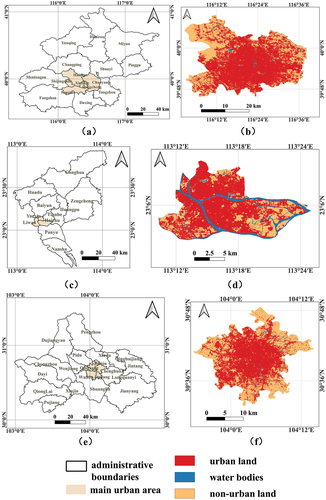
Three typical cities located in China, namely Beijing, Guangzhou, and Chengdu, were selected to evaluate the performance of the SH-CA model. All three cities are at the core of China’s modernization and urbanization policies and have experienced rapid urban expansion over the last several decades. As the industrial, economic, and cultural centers of North China, South China, and West China, respectively, these three distinct cities exhibit complex and unique urban expansion patterns. Therefore, the main urban areas of Beijing, Guangzhou, and Chengdu (abbreviated as BJM, GZM, and CDM, respectively) were selected as study areas. The BJM (Figure 1b) is functionally compact, and urban land and population have grown rapidly over the past 20 years (Liu 2021). The urban land pattern of the GZM (Figure 1d) is basically stable and will be dominated by infill expansion in the long term (Gong et al. 2018). The CDM (Figure 1f) has experienced relatively rapid urban expansion in a “compact circle” pattern (Yu et al. 2022). We argue that the dynamic and complex expansion patterns in these areas provide adequate evidence for performance evaluation.

Figure 1. Locations and 2005 land-use patterns of the study areas. The land uses were reclassified by the China land cover dataset (Yang and Huang 2021). (a) administrative divisions and the main urban area in Beijing. (b) 2005 land use-pattern for the main urban area of Beijing. (c) administrative divisions and the main urban area in Guangzhou. (d) 2005 land use-pattern for the main urban area of Guangzhou. (e) administrative divisions and the main urban area in Chengdu. (f) 2005 land use-pattern for the main urban area of Chengdu.

2.2 Data

Urban expansion data in the study area were extracted from the China Land Cover Dataset (CLCD) (Yang and Huang 2021), which contains land cover maps at 30-m resolution for the entire China. It is suitable for model-performance evaluation because of its high and leading overall mapping accuracy of 79.31%. To reduce the model’s complexity and enhance the model’s adaptability (Liang et al. 2021), we reclassified the nine land cover types in CLCD into three types: water bodies, non-urban land, and urban land (Table 1). Moreover, we analyzed land use transition proportions in the three study areas, and found that the transition of water bodies between 2005 and 2015 cannot be overlooked and the change of urban land was almost negligible (Table 2).

Table 1. Remap table for reclassification of land cover types in the China land cover dataset (Yang and Huang 2021.).

Reclassified types	Original types in CLCD
water bodies	water
non-urban	cropland, forest, shrub, grassland, snow/ice, barren, wetland
urban land	impervious

Table 2. The land use transition proportions in the three study areas from 2005 to 2010 and 2010 to 2015.

Periods	Study area	Transition proportion
		Urban land	Water bodies	Non-urban land
2005–2010	GZM	0.378%	3.544%	18.250%
	BJM	0.070%	21.018%	13.158%
	CDM	0.105%	44.739%	24.345%
2010–2015	GZM	0.337%	2.984%	10.223%
	BJM	0.326%	12.369%	10.225%
	CDM	0.045%	28.059%	18.655%

Four urban expansion maps of the three study areas from 2000, 2005, 2010, and 2015 were selected as experimental data. Various external driving factors play important roles in urban expansion (Liu et al. 2017; Zhang et al. 2019). Several types of driving factors were selected as auxiliary data, including terrain factors (DEM and slope), traffic factors (distance to primary roads, secondary roads, and residential roads), and development factors (GDP and population). Most factors remained unchanged, except for developmental factors. Therefore, two periods of development factors were introduced to mitigate the dynamic problem. All driving factors were resampled to the same resolution of 30 × 30 m to align the urban expansion maps. The driving factors are listed in Table 3.

Table 3. Details of the driving factors included in this study.

Category	Driving factors	Resolution	Data resource	Year
Terrain	DEM	30m	Aster GDEM v2, USGS Earth Explorer (Tachikawa et al. 2011)	2011
	Slope	30m
Development	Population	1km	China population spatial distribution kilometer grid dataset (Xu 2017b)	2005, 2010
	GDP	1km	China GDP spatial distribution kilometer grid dataset (Xu 2017a)	2005, 2010
Traffic	distance to primary roads	30m	OpenStreetMap (Geofabrik 2021)	2021
	distance to secondary roads	30m
	distance to residential roads	30m

3 Methods

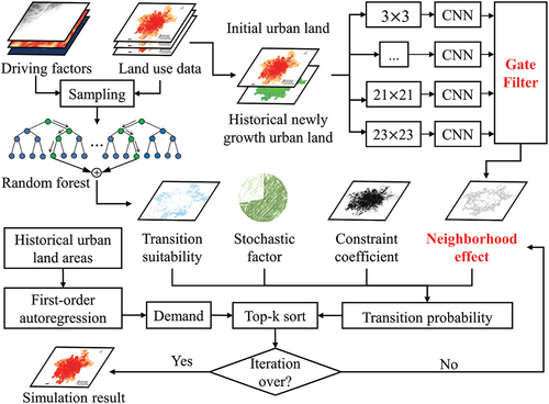
The proposed spatial hierarchical learning module is scalable and can be integrated with CA and its multiple variants. To demonstrate the complete pipeline of urban expansion simulation, a well-designed CA model was combined with a spatial hierarchical learning module to form our SH-CA framework (Figure 2). The SH-CA pipeline was divided into the following parts: (1) Transition suitability modeling by random forest (RF); (2) Training of hierarchical CNNs using land use data and extracted temporal prior knowledge. The aggregated neighborhood effects were obtained using our developed gate filter; (3) Based on transition suitability, stochastic factor, constraint coefficient, and the neighborhood effects, the transition probability was rectified and entered as a parameter in the CA model; and (4) The land-use patterns of future scenarios were predicted by simulation of CA.

Figure 2. Overall framework of the spatial hierarchical learning module based cellular automata (SH-CA).

3.1 Transition suitability modeling

Transition suitability is the driving force of natural and built environments for land-use development. For an individual cell, the value of transition suitability can be calculated from mass-driving factors using a suitable mapping function (Lv et al. 2021). Considering complex input data with nonlinear features, RF is an applicable and powerful mapping function (Zhai et al. 2020). First, we generated representations of the RF inputs based on auxiliary data. Specifically, we organized all driving factors as feature vectors and normalized them to the range [0, 1] using min – max feature scaling. Second, for the K decision trees to be trained, the normalized features are utilized for each individual decision tree. Through Bootstrapping sampling method, an out-of-bag (OOB) dataset and a training dataset are randomly extracted for each tree. The OOB datasets serve to evaluate the generalization capability of the constructed random forest. For the training dataset of the i-th decision tree, a subset of features is randomly selected from the total features. The best feature in this subset is determined for node splitting using the Gini impurity or entropy criterion. This process continues recursively, splitting nodes until the stopping conditions are met, resulting in the completion of the i-th decision tree. Finally, upon the completion of all K decision trees, the classification results for the input features are obtained through voting.

The RF is robust to outliers and nonlinearity in driving factors. For an individual cell $c_i$, various decision trees $f_k,k\in \left[1,K\right]$, are combined to predict its transition suitability value $P_i$ as follows:

(1) $P_i=\frac{{\displaystyle {\sum }_{k=1}^{K}I}\left\{f_k\left(x_i\right)\right\}}{K}$(1)

where $K$ denotes the number of decision trees; $x_i$is the input normalized feature vector of $c_i$; and $I\left\{\cdot \right\}$ denotes the 0–1 indicator function of i-th decision tree. $I\left\{\cdot \right\}$ outputs 1 if the corresponding decision tree predicts that the non-urban land or water bodies located in $c_i$ change to urban land; otherwise, $I\left\{\cdot \right\}$ outputs 0.

3.2 Neighborhood effects learning

3.2.1 Structure of neighborhood

The neighborhood effects emphasize how surrounding cells contribute to the transition of central cells into urban land (Wu 2002). To quantify the neighborhood effects of a central cell $c_i$, a neighborhood function $g\left(\cdot \right)$ is introduced to refine the features from pre-defined neighborhood $Ne\left(c_i\right)$ (Chen, Zhuang, and Liu 2023; Li, Yang, and Liu 2008; Wu et al. 2022; Yang, Li, and Shi 2008) as below:

(2) $\begin{array}{c}{\mathrm{\Omega }}_i=g\left(Ne\left(c_i\right)\right)\end{array}$(2)

where ${\mathrm{\Omega }}_i$ denotes the quantified value of the neighborhood effects.

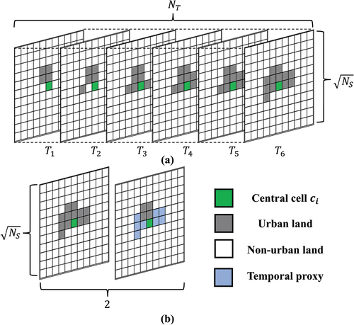
To capture the interaction patterns between the spatial and temporal dimensions, as illustrated in Figure 3a, a common solution is to put $N_S$ spatial neighbors and $N_T$ temporal neighbors into $Ne\left(c_i\right)$. However, for a single central cell $c_i$, $N_S\times N_T$ records are required. This is difficult to implement when the data are incomplete and not evenly sampled in the temporal dimension. We argue that there is a compact proxy refined from $N_T$ temporal neighbors of each single cell, which is sufficient to represent the temporal effect. By concatenating the proxy with the features of $N_S$ spatial neighbors, the requirement for $N_S\times N_T$ records can be simplified to two$\times N_S$ records, thus which mitigating the problem of data hunger. Finally, the structure of the neighborhood $Ne\left(c_i\right)$ can be formalized as a three-dimensional tensor ${\mathcal{X}}_i\in {\mathbb{R}}^{\sqrt{N_S}\times \sqrt{N_S}\times 2}$. As illustrated in Figure 3b, the first channel represents the state of the cells located in $c_i$’s Moore neighborhood, whereas the last channel represents the values of the compact proxy.

Figure 3. The common and proposed neighborhood structures. (a) the common neighborhood structure with $N_T$ temporal neighbors. (b) the proposed neighborhood structure with 2 channels.

3.2.2 Knowledge extraction for compact proxy of temporal neighborhood effects

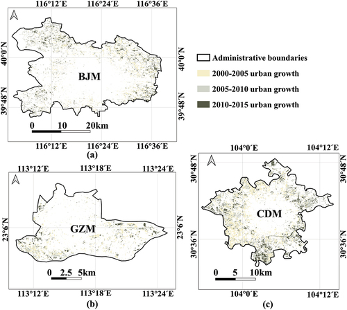
A reliable way to define the compact proxy of temporal neighbors is to determine the predominant mechanism inherent to the temporal process of urban expansion. Based on an in-depth analysis of existing studies, knowledge of historical expansion trends provides prior evidence of urban growth (Gao and O’Neill 2020; Li, Zhou, and Chen 2020; Wang et al. 2021). As shown in Figure 4, new urban growth in each period shows a strong spatial connectivity and can express knowledge of the historical urban expansion trend. This knowledge is suitable for temporal neighborhood effects representation because of the properties of (1) causality, that is, ensuring that the model does not violate the direction of urban expansion; and (2) Markov, that is, only changes between two moments are sufficient for the calculation. Therefore, we quantified the expansion trend of the cell $c_i$ as the compact proxy ${\tau }_i$. Specifically, in this study, if the non-urban land or water bodies located at $c_i$ transferred to the urban land from one historical year to the initial simulation year, then ${\tau }_i=2$; otherwise, ${\tau }_i=1$.

Figure 4. Trends of new urban growth from 2000–2015 in the study areas. (a) trend of BJM. (b) trend of GZM. (c) trend of CDM.

3.2.3 Spatial hierarchical learning module

Based on the pre-defined neighborhood structure information ${\mathcal{X}}_i$, a common way to represent spatial dependence in neighborhood effects of a central cell $c_i$ is to define a proper neighborhood function $g\left(\cdot \right)$

(3) $\begin{array}{c}{\mathrm{\Omega }}_i=g\left({\mathcal{X}}_i\right)\end{array}$(3)

The classical and basic expression (i.e. mean):

(4) $\begin{array}{c}g\left({\mathcal{X}}_i\right)=\frac{{\sum }_{u,v}^{\sqrt{N_S}}Con\left({\mathcal{X}}_i\left(u,v,1\right)=urbanland\right)}{N_S-1}\end{array}$(4)

where ${\sum }_{u,v}^{\sqrt{N_S}}Con\left({\mathcal{X}}_i\left(u,v,1\right)=urbanland\right)$ represents the total number of urban land cells in the neighborhood. Introducing the weights ${\theta }_{u,v}$ and ${\theta }_m$ (weighted sum), we can obtain the weighted representations of the spatial dependence and the historical expansion trends:

(5) $\begin{array}{c}g\left({\mathcal{X}}_i\right)={\sum }_{u,v}^{\sqrt{N_S}}{\theta }_{u,v}{\sum }_{m=1}^2{\theta }_m{\mathcal{X}}_i\left(u,v,m\right)\end{array}$(5)

where u and v represent cell $c_{uv}$’s row and column indices in neighborhood of cell $c_i$. m can take the value 1 or 2. ${\mathcal{X}}_i\left(u,v,1\right)$ denotes the state of $c_{uv}$, while ${\mathcal{X}}_i\left(u,v,2\right)$ represents the value of the compact proxy for $c_{uv}$.

With weight adaption, the parameterized filter $g_{\theta }^{\sqrt{N_S}}$equipped with a receptive field with the size of $\sqrt{N_S}$ was defined. The equation is equal to the convolution between parameterized filter $g_{\theta }$ and the neighborhood structure information ${\mathcal{X}}_i$

(6) $\begin{array}{c}g\left({\mathcal{X}}_i\right)=g_{\theta }^{\sqrt{N_S}}\ast {\mathcal{X}}_i\end{array}$(6)

Utilizing multiple filters $g_{{\theta }_j}^{\sqrt{N_S}}$ with different trainable weights ${\theta }_j$ to enhance the learning ability, we obtain

(7) $\begin{array}{c}g\left({\mathcal{X}}_i\right)=\underset{j}{\cup }{g}_{{\theta }_j}^{\sqrt{N_S}}\ast {\mathcal{X}}_i\end{array}$(7)

To capture the nonlinear interaction relationship between the spatial dependence and the historical expansion trends, the activation function $\sigma \left(\cdot \right)$ is added

(8) $\begin{array}{c}g\left({\mathcal{X}}_i\right)=\sigma \left(\underset{j}{\cup }{g}_{{\theta }_j}^{\sqrt{N_S}}\ast {\mathcal{X}}_i\right)\end{array}$(8)

Thus far, the designed $g\left({\mathcal{X}}_i\right)$ has the advantages of self-adaption, high-dimensional feature extraction, and nonlinear complex relationship modeling. Fortunately, with the same basic structure as $g\left({\mathcal{X}}_i\right)$ and a high computational efficiency, CNNs are powerful tools for constructing $g\left({\mathcal{X}}_i\right)$. Therefore, we designed an efficient and lightweight CNN to model the spatio-temporal interaction between the spatial dependence and the historical expansion trends in neighborhood effects. The structure of the lightweight CNN, which contains two core convolutional layers, is shown in Figure 5. The kernel size of the first convolutional layer is 1, which is aimed at enhancing the feature dimension to mine the relationship between the current land use and the historical expansion trends and obtaining feature ${{\mathcal{X}}_i}^1$

(9) $\begin{array}{c}{{\mathcal{X}}_i}^1=\sigma \left(\underset{j}{\cup }{g}_{{\theta }_j}^1\ast {\mathcal{X}}_i\right)\end{array}$(9)

Figure 5. Structure of the lightweight CNN for neighborhood size k.

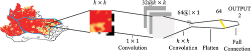
The kernel size of the second convolutional layer is $k$, which is the same as the neighborhood size, and is aimed at modeling the spatial dependence of the enhanced spatio-temporal feature and obtaining feature ${{\mathcal{X}}_i}^2$

(10) $\begin{array}{c}{{\mathcal{X}}_i}^2=\sigma \left(\underset{j}{\cup }{g}_{{\theta }_j}^k\ast {{\mathcal{X}}_i}^1\right)\end{array}$(10)

Then, the interacting spatio-temporal neighborhood effects ${\mathrm{\Omega }}_{k,i}$ for neighborhood size k is regressed by a fully connected layer. The quantification of ${\mathrm{\Omega }}_{k,i}$ involves mapping the features ${{\mathcal{X}}_i}^2$to the value of neighborhood transition potential (NTP) as follows:

(11) $\begin{array}{c}{\mathrm{\Omega }}_{k,i}=\sigma \left({\sum }_{j=1}^n{\theta }_j{{\mathcal{X}}_i}^2\left(j\right)\right)\end{array}$(11)

Since the ${\mathrm{\Omega }}_{k,i}$ only expresses the neighborhood effects of $c_i$ at this particular scale, influenced by the scale effect, the NTPs at different scales are biased, which exhibits as neighborhood sensitivity. As the cells with high NTPs in a neighborhood size may have lower NTPs at other neighborhood sizes, this can cause uncertainty in NTP characterization, leading to randomness in the simulation results. Therefore, we developed a spatial hierarchical learning module to address multiscale information learning and aggregation. Hierarchical CNNs stack $K$ lightweight CNNs at different scales $k$ in parallel, and a gate filter $GaF\left(\cdot \right)$ was introduced to aggregate the NTPs $\left\{{\mathrm{\Omega }}_{k,i},k\in \left[1,K\right]\right\}$ from multiple scales. The gate filter was supposed to retain important information for a long time (Figure 6), similar to the gate mechanism in Long Short-Term Memory (LSTM) Networks (Hochreiter and Schmidhuber 1997), and minimize the low signal and highlight the high signal, similar to the high-pass filtering in signal processing. Therefore, the gate filter is defined as

Figure 6. Schematic framework of the spatial hierarchical learning module. The module comprises multiple lightweight CNNs and a gate filter to learn and aggregate multiscale neighborhood effects.

(12) $\begin{array}{c}{\mathrm{\Omega }}_i=GaF\left(\underset{i}{\cup }{\mathrm{\Omega }}_{k,i}\right)=\prod _{k=1}^K{\mathrm{\Omega }}_{k,i}\end{array}$(12)

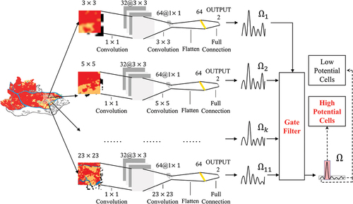
where ${\mathrm{\Omega }}_i$ refers to multiscale neighborhood effects of cell i, and $K$ is number of neighborhood sizes.

Intuitively, the value of ${\mathrm{\Omega }}_{k,i}$ ranges from 0 to 1, which means that the NTP closed to 1 at each neighborhood scale also needs to be closed to 1 after filtering; otherwise, it will be closed to 0. Therefore, the gate filter can identify cells with high NTPs for each neighborhood size.

3.3 Simulation of the SH-CA model

CA models for urban expansion consist of top-down and bottom-up modules (Liu et al. 2017; Verburg and Overmars 2009; Verburg et al. 2002). For the top-down module, a first-order autoregressive method was used to model the Markov processes of land-use area changes (He et al. 2018; Wu et al. 2019). Meanwhile, the bottom-up module controls the transition of the cells from a local perspective to satisfy the macroscopic demand, which is dominated by the transition probability. The transition probability consists of four parts: transition suitability, neighborhood effects, constraint coefficient, and stochastic factor (Li and Yeh 2002; Zhai et al. 2020). In this study, the transition suitability was calculated using RF, and the neighborhood effects were determined using the spatial hierarchical learning module. The constraint coefficient constrains specific land use in specific areas not to change [e.g. urban land (Schaldach et al. 2011), water bodies (Xie et al. 2020), ecological reserves (Liu et al. 2017)]. According to the transition trends of historical land-use data, the baseline scenario in this study constrained existing urban land from remaining unchanged. Considering the stochasticity and uncertainty in land-use change, the stochastic disturbance term $RA$ was introduced in the CA models as a stochastic factor (Feng and Liu 2013; Liao et al. 2016; White and Engelen 1993; Xie et al. 2020; Zhai et al. 2020). Thus, the transition probability can be expressed as

(13) $\begin{array}{c}T{P}_i^t=P_i\times {\mathrm{\Omega }}_i^t\times con\left(S_i^t\right)\times RA\end{array}$(13)

where $T{P}_i^t$ is the transition probability of cell i at time t; $P_i$ is the transition suitability of cell i; ${\mathrm{\Omega }}_i^t$ refers to the neighborhood effects of cell i at time t; $con\left(S_i^t\right)$ refers to the constraint coefficient of state of cell i; RA is the stochastic factor, $RA=1+{\left(-lny\right)}^{\alpha }$, where $y$ is a range random value between 0 and 1; and $\alpha$ is an integer ranging from 1 to 10 that controls the effect of stochastic perturbation.

For each iteration in the SH-CA model, $T{P}_i^t$ will be updated with ${\mathrm{\Omega }}_i^t$ and $con\left(S_i^t\right)$. Based on the urban land demand for this iteration, the corresponding number of cells with a higher transition probability was selected to develop into urban land. The iterations stop when the preset time point is reached, and the SH-CA model exports the simulation results.

3.4 Model evaluation

In this study, 80,000 samples were randomly selected for each transition-type code to construct the sample sets, of which 80% were used for training and 20% for validation. For transition suitability modeling, RF uses CART trees with a number of 50. For the constraint coefficient, if cell i’s state is urban land, the value of$con\left(S_i^t\right)$ is 1; otherwise, it is 0. For neighborhood effects learning, the neighborhood sizes ranged from 3 to 23, with a gap of 2 (11 total sizes), considering the extent of the urban block (Wang and Zang 2018). For the hyperparameters of the hierarchical CNNs, the hidden sizes of the first and second layers were set to 32 and 64, respectively. The learning rate was set to 0.001. The batch sizes were set to 16, 16, and 32 for the GZM, BJM, and CDM, respectively. The Adam optimizer and early stopping techniques were applied. To better assess the validity of the SH-CA model, the stochastic factor was excluded to prevent instability of the assessment when conducting experimental comparisons; however, it was considered in future scenario simulation experiments.

Four other CA models (LR-CA, SVM-CA, RF-CA, and ANN-CA) were used to compare the performance of the SH-CA model, with RF-CA differing from SH-CA in neighborhood effects learning part only, and the four comparison models utilize the classic neighborhood function and the gate filter. The logistic regression (LR) optimization algorithm employed is “newton-cg.” The support vector machine (SVM) utilizes the radial basis function (RBF) kernel. The hidden layers of the artificial neural network (ANN) comprise a 32-dimensional fully connected layer and a 64-dimensional fully connected layer.

To evaluate the urban expansion simulation results, the overall accuracy (OA), Kappa coefficient, and figure of merit (FoM) were used to assess the performance of the SH-CA model. OA refers to the proportion of correctly simulated cells compared to the total number of cells. Considering sample imbalance, the Kappa coefficient measures the consistency of the simulation results with real land use (Cohen 1960; Lv et al. 2021). Considering the stability of most cells, FoM focuses on the changes between simulated and observed land use (Liu et al. 2017; Pontius et al. 2008). The equations for these indicators are as follows:

(14) $\begin{array}{c}OA={\sum }_k^m\frac{N_{kk}}{sum}\times 100\mathrm{\%}\end{array}$(14)

(15) $\begin{array}{c}{P}_e=\frac{{\sum }_k^m{N}_k\times M_k}{su{m}^2}\end{array}$(15)

(16) $\begin{array}{c}Kappa=\frac{OA-P_e}{1-P_e}\end{array}$(16)

(17) $\begin{array}{c}FoM=\frac{B}{A+B+C+D}\end{array}$(17)

where $sum$ represents the total number of cells, m is the number of land-use types, $N_{kk}$ denotes the number of cells correctly predicted for the k-th land use type, $N_k$ denotes the number of cells simulated for the k-th land use type, $M_k$denotes the number of cells of k-th land use type, $P_e$ is the expected consistency, A is the number of error cells that changed but were simulated as unchanged, B is the number of cells that changed and were correctly simulated, C is the number of error cells that changed but were simulated as changing to incorrect land use types, and D is the number of error cells that remained unchanged but were simulated as changed. The model with the largest values of the three indices showed the best performance. Generally, most of cells remain unchanged during the actual process of urban expansion, which will result in the OA and Kappa coefficients of different CA models being very closed. Therefore, it is essential to pay more attention to the FoM.

4 Results

4.1 Implementation and comparison

The proposed SH-CA model was applied to the BJM, GZM, and CDM to simulate urban land in 2015. The evaluation indicators of simulation results based on SH-CA model and the four comparison models are shown in Table 4. The FoM of SH-CA increased by 52.0%, 67.3%, 101.8%, and 66.1% relative to RF-CA, LR-CA, SVM-CA, and ANN-CA in the GZM, respectively, which was much better than the comparison models in the three study areas. Because of the small amount of incremental urban land in the main urban areas, better simulation results have limited gain for OA and Kappa. As the FoM can evaluate the expansion between simulated and observed urban land and has significant improvement with the SH-CA model, the improvement could be attributed to the powerful fitting capabilities of CNNs for the spatio-temporal interaction between the spatial dependence and the historical expansion trends in neighborhood effects.

Table 4. Evaluation indicators (OA, Kappa and FoM) of simulation results based on different models in GZM, BJM, and CDM.

Model	GZM			BJM			CDM
	OA	Kappa	FoM	OA	Kappa	FoM	OA	Kappa	FoM
SH-CA	0.9672	0.9250	0.1231	0.9563	0.8899	0.1485	0.9201	0.8029	0.2189
RF-CA	0.9644	0.9187	0.0810	0.9530	0.8814	0.1095	0.9127	0.7842	0.1747
LR-CA	0.9638	0.9172	0.0736	0.9530	0.8814	0.1097	0.9121	0.7827	0.1715
SVM-CA	0.9628	0.9150	0.0610	0.9531	0.8817	0.1110	0.9127	0.7844	0.1751
ANN-CA	0.9638	0.9173	0.0741	0.9530	0.8815	0.1098	0.9126	0.7841	0.1746

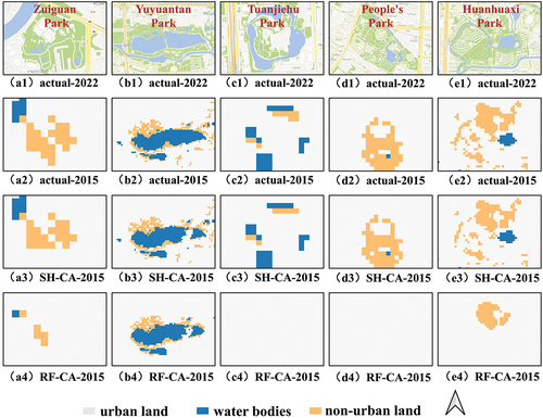
Because RF-CA has the best overall performance among the comparison methods, actual land use, SH-CA simulation results, and RF-CA simulation results are shown in Figure 7. Overall, the RF-CA simulation results were more homogeneous relative and directionless than the SH-CA, failing to reflect the complexity of the main urban sprawl. According to actual historical expansion trends and land use functions, some important parks and attractions in the city have hardly developed as urban land. However, the open spaces in Zuiguan Park in Guangzhou, Yuyuantan Park, Tuanjiehu Park in Beijing, and People’s Park and Huanhuaxi Park in Chengdu disappeared or were extensively reduced in the RF-CA simulation results, whereas they remained unchanged in the SH-CA simulation results (Figure 8). This demonstrates that the SH-CA model is suitable for mining the complex spatio-temporal interaction between the spatial dependence and the historical expansion trends in neighborhood effects.

Figure 7. Actual land use and simulation results of the SH-CA and RF-CA for 2015. (a, d, g) Overall and local actual land use for GZM, BJM and CDM. (b, e, h) Overall and local simulation results of the SH-CA model for GZM, BJM and CDM. (c, f, i) Overall and local simulation results of the RF-CA model for GZM, BJM and CDM.

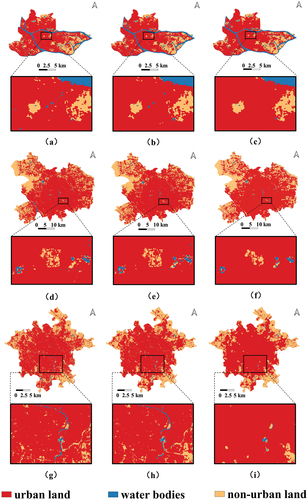
Figure 8. Details of actual land function in 2022 from online mapping service of tianditu (https://www.tianditu.gov.cn/), actual land use in 2015, and simulated land use of the SH-CA and RF-CA models. (a1–a4) Details of the Zuiguan Park in Guangzhou. (b1–b4) Details of the Yuyuantan Park in Beijing. (c1–c4) Details of the Tuanjiehu Park in Beijing. (d1–d4) Details of the People’s Park in Chengdu. (e1–e4) Details of the Huanhuaxi Park in Chengdu.

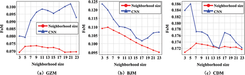
We removed the spatial hierarchical learning module and modeled the neighborhood effects of a single neighborhood size separately by visualizing the FoM of each neighborhood size based on the neighborhood function and CNN (Figure 9). The curves of CNNs in all three studied areas lied above the neighborhood functions, indicating that CNN was better than the neighborhood function. The FoM values of the SH-CA model were greater than 20.7%, 20.1%, and 17.7% of the peaks of the three curves of CNN (GZM: 0.1020, BJM: 0.1236, CDM: 0.1860), respectively, demonstrating the effectiveness of the gate filter.

Figure 9. FoMs of each neighborhood size based on the neighborhood function and CNN. (a) FoMs of GZM. (b) FoMs of BJM. (c) FoMs of CDM.

To further demonstrate the superiority of the gate filter (hereafter, Filter-1), we designed a comparison strategy, Filter-2. Similar to the RF algorithm in ensemble learning, the decision outcome was determined by decision tree voting or based on the mean of the results of the decision trees. Specifically, the gate filter of Filter-2 averaged the NTPs over all scales to select cells with high NTPs after filtering

(18) $\begin{array}{c}{\mathrm{\Omega }}_i=GaF\left(\underset{i}{\cup }{\mathrm{\Omega }}_{k,i}\right)=\frac{{\sum }_{k=1}^K{\mathrm{\Omega }}_{k,i}}{K}\end{array}$(18)

We repeated the experiment shown in Table 4 based on Filter-2 (namely with SH-CA*, RF-CA*, LR-CA*, SVM-CA*, and ANN-CA*). As shown in Table 5, the same conclusion was obtained, that is, the proposed SH-CA model significantly outperformed the other comparison CA models. The simulation results for Filter-2 remained different from those of Filter-1. We speculate that the gate filter of Filter-1 was stricter than that of Filter-2; therefore, the cells with high NTPs filtered by Filter-2 May have more noise and interference. In some cases, it is difficult to prioritize the development of cells with a high development potential. Consequently, Filter-1 in the proposed SH-CA can better filter out cells that may not have high NTPs and correctly select cells to develop into urban land, thus integrating multiscale information and mitigating neighborhood sensitivity.

Table 5. Evaluation indicators (OA, Kappa and FoM) of the simulation results based on different models modified by Filter-2 in GZM, BJM, and CDM.

Model	GZM			BJM			CDM
	OA	Kappa	FoM	OA	Kappa	FoM	OA	Kappa	FoM
SH-CA*	0.9664	0.9231	0.1111	0.9543	0.8849	0.1264	0.9173	0.7961	0.2025
RF-CA*	0.9639	0.9173	0.0730	0.9525	0.8801	0.1049	0.9124	0.7837	0.1736
LR-CA*	0.9605	0.9096	0.0295	0.9522	0.8793	0.1013	0.9080	0.7728	0.1495
SVM-CA*	0.9606	0.9099	0.0314	0.9524	0.8799	0.1048	0.9106	0.7793	0.1635
ANN-CA*	0.9626	0.9145	0.0574	0.9526	0.8804	0.1059	0.9104	0.7788	0.1626

4.2 Simulation of future scenarios

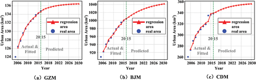
As urbanization enters its later stages, the limited land available for urban development continues to shrink, and urban expansion gradually slows. The regression areas of urban land demand from 2006 to 2030 utilizing the first-order autoregressive method in the study areas are shown in Figure 10. The slopes of the three curves gradually became smaller and leveled off, with the urban land area increasing by 7.80%, 3.66%, and 13.62% in the BJM, GZM, and CDM, respectively, from 2010 to 2030, which is in line with the law of real urban land expansion.

Figure 10. The actual areas and regression areas ($k{m}^2$) of urban land demand. The green dash lines mean that regression areas from 2006–2030 are regressed based on real areas from 2005–2015. (a) urban land demand of GZM. (b) urban land demand of BJM. (c) urban land demand of CDM.

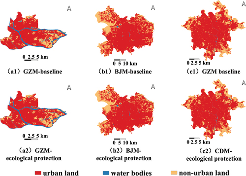
In this study, we designed two scenarios and applied the proposed SH-CA model to simulate urban land patterns from 2010 to 2030. The first scenario was a baseline scenario based on historical urban development trends. Guided by China’s ecologically sustainable development strategy, urban development must be combined with ecological protection. Therefore, the second scenario, the ecological protection scenario requires that water bodies remain unchanged and aim to protect urban open spaces, such as rivers, ecological parks, and attractions, in the city.

As shown in Figure 11, by comparing the simulation results of the baseline and ecological protection scenarios, the land-use patterns were generally similar in the study areas. Although a small portion of water bodies is occupied by urban land in the baseline scenario, the majority of water bodies were preserved. The observation suggested that there may be implicit knowledge of water bodies protection embedded in the spatial hierarchical learning module.

Figure 11. Simulation results of the baseline scenario and ecological protection scenario for 2030. (a1-c1) simulation results of the baseline scenario for GZM, BJM, and CDM. (a2-c2) simulation results of the ecological protection scenario for GZM, BJM, and CDM.

In an overview of the changes over 20 years, urban expansion in the GZM from 2010 to 2030 was relatively slow. Since the urban center of gravity in Guangzhou moved to the Tianhe district, the Yuexiu and Liwan districts are now old urban areas. In the BJM, the Chaoyang District has experienced the most rapid development among the six districts. Compared to the current level of economic development in Beijing, the Chaoyang District has the highest GDP value. Meanwhile, all administrative districts in the CDM have showed some degree of urban expansion from 2010 to 2030, with Wuhou District being the most notable, thus showing huge potential for future development. Overall, the urban functions of the main urban areas are gradually enriched as urbanization progresses until land resources are almost fully utilized. Then, the function relocation or the urban centers of gravity shift will be considered.

5 Discussion

5.1 Neighborhood size combination sensitivity analysis

Neighborhood size directly determines the source of information for neighborhood effects learning. However, there are correlations and dependencies across the information from different neighborhood sizes. Moreover, the efficiency of the model decreases as the number of neighborhood sizes increase. Therefore, based on the different neighborhood size combinations, we designed three groups of comparison experiments with different lengths and gaps of the combinations, namely Comb-1, Comb-2, and Comb-3. The combination configurations and FoMs of Comb-1, Comb-2, and Comb-3 are listed in Table 6.

Table 6. FoMs of simulation results based on SH-CA models under Comb-1, Comb-2, and Comb-3 in GZM, BJM, and CDM.

Combination type	Neighborhood sizes	GZM	BJM	CDM
Comb-1	3,5,7,9,11,13,15	0.1205	0.1432	0.2129
	7,9,11,13,15,17,19	0.1184	0.1390	0.2140
	11,13,15,17,19,21,23	0.1139	0.1393	0.2145
Comb-2	3,5,7	0.1014	0.1348	0.2076
	9,11,13	0.1140	0.1272	0.2048
	15,17,19	0.1111	0.1233	0.2042
	19,21,23	0.1109	0.1257	0.2042
Comb-3	3,7,11,15,19,23	0.1152	0.1439	0.2185
	3,11,15,23	0.1156	0.1400	0.2175
	5,9,13,17,21	0.1230	0.1383	0.2164

Compared to the above FoMs based on the gate filter, single neighborhood size in Figure 9, Comb-1 and Comb-2, the increase in the total number of neighborhood sizes improved the performance of the SH-CA model. Combined with Comb-3, the highest FoMs appeared in Comb-3 of the three groups of comparison experiments and were very close to the FoMs based on the 11 neighborhood sizes. Therefore, sampling the neighborhood size at an interval of 120 m was a suitable choice for the tradeoff between accuracy and efficiency.

The study areas have different neighborhood combination tendencies; for example, the GZM prefers moderately large neighborhood size combinations, the BJM prefers small neighborhood size combinations, and the CDM prefers moderately small neighborhood size combinations. Consequently, quantitative combination of the smallest number of neighborhood sizes to achieve the highest possible accuracy and efficiency is worth exploring in the future.

5.2 NTPs’ distribution analysis

Although the effectiveness of the gate filter has been proven above, it is more important to address why the strategy can mitigate neighborhood sensitivity. In all the comparison experiments, the transition probability drives land conversion. Among the components of transition probability, transition suitability and constraint coefficient were constant during the iterations, and the stochastic factor was removed to ensure stability of the comparison experiments. Therefore, the role played by the neighborhood effects in the SH-CA model warrants further exploration.

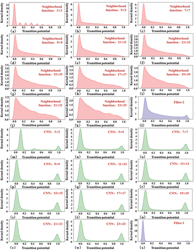
Taking the CDM as an example (GZM and BJM are similar to the CDM), the NTPs’ kernel density distributions in the neighborhood function for single neighborhood size, CNN for single neighborhood size, Filter-1 and Filter-2 after the first iteration are shown in Figure 12. The kernel density distributions of the neighborhood functions typically exhibit skewed distributions without clear boundaries to distinguish between cells with high and low NTPs. This problem was solved using CNNs that exhibit bimodal distributions.

Figure 12. Kernel density distributions of the NTPs based on different neighborhood functions, CNNs and gate filters. (a-k) neighborhood functions with neighborhood size: 3, 5, 7, 9, 11, 13, 15, 17, 19, 21 and 23. (m-w) CNNs with neighborhood size: 3, 5, 7, 9, 11, 13, 15, 17, 19, 21 and 23. (l, x) Filter-2 and Filter-1.

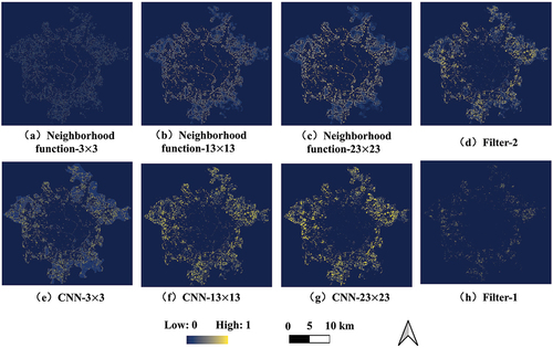
The NTPs’ spatial distributions in Moore 3 × 3, Moore 13 × 13, and Moore 23 × 23 of the neighborhood functions and the CNNs, Filter-1, and Filter-2 are shown in Figure 13. Cells with high NTPs of the neighborhood functions were mainly located at existing urban land boundaries without the directionality of urban expansion. This was improved in the CNNs after considering the spatio-temporal interaction between the spatial dependence and the historical expansion trends.

Figure 13. Spatial distributions of the NTPs based on different neighborhood functions, CNNs and gate filters. (a-c) neighborhood functions with neighborhood size: 3, 13 and 23. (e-g) CNNs with neighborhood size: 3, 13 and 23. (d, h) Filter-2 and Filter-1.

However, the number of cells with high NTPs was much larger than that of the small urban land demand, making it necessary to further select cells using the gate filter. Comparing Filter-1 and Filter-2 in Figures 12 and 13, the filtering capability of Filter-2 was weaker than that of Filter-1, resulting in the filtered cells still exceeding the demand and the existence of a large amount of noise. Although Filter-1 performed better in these main urban areas, this does not mean that Filter-2 was inferior. As the Filter-1’s excellent performance is attributed to its harsh filtering rule, which suits the low demand for urban expansion in the main urban areas, Filter-2 May outperform Filter-1 in regions with large urban expansion.

5.3 Analysis of scalability

The development of the spatial hierarchical learning module is the main contribution of this study. We hope that this is not only applicable to the current framework of the SH-CA model but also scalable to other CA models. To investigate its scalability on existing models, we applied it to the LR-CA, ANN-CA, and SVM-CA models (namely LR-CA**, SVM-CA**, and ANN-CA**, respectively) (Table 7). A comparison of the simulation results in Table 4 reflects a significant enhancement after applying the contributions of this study. Although the LR-CA**, SVM-CA**, and ANN-CA** models were slightly inferior to the proposed SH-CA model, this was attributed to the difference in the learning ability for transition suitability among the different machine learning methods used in this study. Overall, the proposed spatial hierarchical learning module exhibited highly scalable potential and broad application prospects in CA models.

Table 7. Comparison of the simulation results based on LR-CA**, SVM-CA**, and ANN-CA** indicated by OA, Kappa and FoM in GZM, BJM, and CDM.

Study area	Indicators	LR-CA**	SVM-CA**	ANN-CA**
GZM	OA	0.9671	0.9671	0.9672
	Kappa	0.9247	0.9247	0.925
	FoM	0.1212	0.1209	0.1231
BJM	OA	0.956	0.9562	0.956
	Kappa	0.889	0.8897	0.8891
	FoM	0.1446	0.1475	0.1447
CDM	OA	0.9198	0.9201	0.9199
	Kappa	0.8022	0.803	0.8025
	FoM	0.2172	0.219	0.218

6 Conclusion

Neighborhood effects serve as the external driving force in CA models for simulating urban expansion. However, previous studies have undervalued the geospatial information of neighborhood effects in spatio-temporal dimensions. Moreover, neighborhood sensitivity is commonly criticized in CA models. To address these challenges, we developed an SH-CA model powered by a spatial hierarchical learning module and applied the SH-CA model in three distinct Chinese urban areas. The results demonstrate that the proposed SH-CA model not only simulates detailed and realistic urban land pattern but also exhibits superior performance than comparative CA models. In addition, we designed experiments to thoroughly analyze the spatial hierarchical module. The results reveal the module’s robust capacity to model the spatio-temporal interaction in neighborhood effects and effectively handle the neighborhood sensitivity, and strong scalability to existing CA models to significantly improve their performance.

Despite the achievements of the SH-CA model, there are several limitations that require further investigation. First, a limited number of driving factors may not fully capture the complexity of transition suitability. Future studies will consider introducing additional dynamic driving factors. Second, the selection of neighborhood sizes and ranges was based on empirical knowledge, which burdened the workload of the model application. Obtaining these parameters adaptively based on land-use patterns will be concerned in future studies. In addition, urban expansion trends may change with the introduction of new governmental and national policies, which weakened the applicability of the model. Modeling dynamics based on policies is a critical challenge for future research.

Data and codes availability statement

The data and codes that support the findings of this study are available on figshare.com with the identifier [DOI: https://doi.org/10.6084/m9.figshare.22183417].

Acknowledgments

This work was carried out in part using computing resources at the High-Performance Computing Platform of Central South University.

Disclosure statement

No potential conflict of interest was reported by the author(s).

Additional information

Funding

This work was supported by the National Natural Science Foundation of China (NSFC), [42171459, 42071452]; the Hunan Provincial Innovation Foundation for Postgraduate [CX20230177]; the Fundamental Research Funds for the Central Universities of Central South University [2023ZZTS0093].

References

- Aburas, M. M., Y. M. Ho, M. F. Ramli, and Z. H. Ash’aari. 2016. “The Simulation and Prediction of Spatio-Temporal Urban Growth Trends Using Cellular Automata Models: A Review.” International Journal of Applied Earth Observation and Geoinformation 52:380–22. https://doi.org/10.1016/j.jag.2016.07.007.
- Angel, S., J. Parent, D. L. Civco, A. Blei, and D. Potere. 2011. “The Dimensions of Global Urban Expansion: Estimates and Projections for All Countries, 2000–2050.” Progress in Planning 75 (2): 53–107. https://doi.org/10.1016/j.progress.2011.04.001.
- Chen, G., X. Li, X. Liu, Y. Chen, X. Liang, J. Leng, X. Xu, et al. 2020. “Global Projections of Future Urban Land Expansion Under Shared Socioeconomic Pathways.” Nature Communications 11 (1): 537. https://doi.org/10.1038/s41467-020-14386-x.
- Chen, G., H. Zhuang, and X. Liu. 2023. “Cell-Level Coupling of a Mechanistic Model to Cellular Automata for Improving Land Simulation.” GIScience & Remote Sensing 60 (1): 21 66443. https://doi.org/10.1080/15481603.2023.2166443.
- Cohen, J. 1960. “A Coefficient of Agreement for Nominal Scales.” Educational and Psychological Measurement 20 (1): 37–46. https://doi.org/10.1177/001316446002000104.
- Dahal, K. R., and T. E. Chow. 2015. “Characterization of Neighborhood Sensitivity of an Irregular Cellular Automata Model of Urban Growth.” International Journal of Geographical Information Science 29 (3): 475–497. https://doi.org/10.1080/13658816.2014.987779.
- Feng, Y., and Y. Liu. 2013. “A Heuristic Cellular Automata Approach for Modelling Urban Land-Use Change Based on Simulated Annealing.” International Journal of Geographical Information Science 27 (3): 449–466. https://doi.org/10.1080/13658816.2012.695377.
- Feng, Y., and X. Tong. 2019. “Incorporation of Spatial Heterogeneity-Weighted Neighborhood into Cellular Automata for Dynamic Urban Growth Simulation.” GIScience & Remote Sensing 56 (7): 1024–1045. https://doi.org/10.1080/15481603.2019.1603187.
- Fotheringham, A. S., and D. W. Wong. 1991. “The Modifiable Areal Unit Problem in Multivariate Statistical Analysis.” Environment and Planning A 23 (7): 1025–1044. https://doi.org/10.1068/a231025.
- Gao, J., and B. C. O’Neill. 2020. “Mapping Global Urban Land for the 21st Century with Data-Driven Simulations and Shared Socioeconomic Pathways.” Nature Communications 11 (1): 2302. https://doi.org/10.1038/s41467-020-15788-7.
- Geofabrik. 2021. “Data From: OpenStreetmap Data Downloads (Dataset)” . OpenStreetMap Contributors. Accessed January 1, 2022. http://download.geofabrik.de/asia/china.html.
- Gong, J., Z. Hu, W. Chen, Y. Liu, and J. Wang. 2018. “Urban Expansion Dynamics and Modes in Metropolitan Guangzhou, China.” Land Use Policy 72:100–109. https://doi.org/10.1016/j.landusepol.2017.12.025.
- Goodchild, M. F. 2004. “The Validity and Usefulness of Laws in Geographic Information Science and Geography.” Annals of the Association of American Geographers 94 (2): 300–303. https://doi.org/10.1111/j.1467-8306.2004.09402008.x.
- Guan, X., H. Wei, S. Lu, Q. Dai, and H. Su. 2018. “Assessment on the Urbanization Strategy in China: Achievements, Challenges and Reflections.” Habitat International 71:97–109. https://doi.org/10.1016/j.habitatint.2017.11.009.
- He, J., X. Li, Y. Yao, Y. Hong, and J. Zhang. 2018. “Mining Transition Rules of Cellular Automata for Simulating Urban Expansion by Using the Deep Learning Techniques.” International Journal of Geographical Information Science 32 (10): 2076–2097. https://doi.org/10.1080/13658816.2018.1480783.
- Hochreiter, S., and J. Schmidhuber. 1997. “Long Short-Term Memory.” Neural Computation 9 (8): 1735–1780. https://doi.org/10.1162/neco.1997.9.8.1735.
- Işınkaralar, O. 2023. “Simulation of Urban Growth’s Pressure on Urban Blue-Green Space Using the CORINE Database for Kocaeli, Türkiye.” Forestist. https://doi.org/10.5152/forestist.2023.22077.
- Isinkaralar, O., and C. Varol. 2023. “A Cellular Automata-Based Approach for Spatio-Temporal Modeling of the City Center as a Complex System: The Case of Kastamonu, Türkiye.” Cities 132:104073. https://doi.org/10.1016/j.cities.2022.104073.
- Isinkaralar, O., C. Varol, and D. Yilmaz. 2022. “Digital Mapping and Predicting the Urban Growth: Integrating Scenarios into Cellular Automata—Markov Chain Modeling.” Applied Geomatics 14 (4): 695–705. https://doi.org/10.1007/s12518-022-00464-w.
- Jelinski, D. E., and J. Wu. 1996. “The Modifiable Areal Unit Problem and Implications for Landscape Ecology.” Landscape Ecology 11 (3): 129–140. https://doi.org/10.1007/BF02447512.
- Kamusoko, C., and J. Gamba. 2015. “Simulating Urban Growth Using a Random Forest-Cellular Automata (RF-CA) model.” ISPRS International Journal of Geo-Information 4 (2): 447–470. https://doi.org/10.3390/ijgi4020447.
- Liang, X., Q. Guan, K. C. Clarke, S. Liu, B. Wang, and Y. Yao. 2021. “Understanding the Drivers of Sustainable Land Expansion Using a Patch-Generating Land Use Simulation (PLUS) Model: A Case Study in Wuhan, China.” Computers, Environment and Urban Systems 85:101569. https://doi.org/10.1016/j.compenvurbsys.2020.101569.
- Liao, J., L. Tang, G. Shao, X. Su, D. Chen, and T. Xu. 2016. “Incorporation of Extended Neighborhood Mechanisms and Its Impact on Urban Land-Use Cellular Automata Simulations.” Environmental Modelling & Software 75:163–175. https://doi.org/10.1016/j.envsoft.2015.10.014.
- Li, Y., Y. Gong, Z. Zhang, and C. Feng. 2018. “On the Neighborhood Patterns of Urban Land Use Using Vector Grids.” Acta Geographica Sinica 73 (11): 2236–2249. https://doi.org/10.11821/dlxb201811014.
- Liu, C. 2021. “Impervious Surface Extraction and Urban Expansion Analysis Based on Time Series.” Master diss, China University of Geosciences.
- Liu, X., X. Liang, X. Li, X. Xu, J. Ou, Y. Chen, S. Li, S. Wang, and F. Pei. 2017. “A Future Land Use Simulation Model (FLUS) for Simulating Multiple Land Use Scenarios by Coupling Human and Natural Effects.” Landscape and Urban Planning 168:94–116. https://doi.org/10.1016/j.landurbplan.2017.09.019.
- Li, X., Q. Yang, and X. Liu. 2008. “Discovering and Evaluating Urban Signatures for Simulating Compact Development Using Cellular Automata.” Landscape and Urban Planning 86 (2): 177–186. https://doi.org/10.1016/j.landurbplan.2008.02.005.
- Li, X., and A. G. O. Yeh. 2002. “Neural-Network-Based Cellular Automata for Simulating Multiple Land Use Changes Using GIS.” International Journal of Geographical Information Science 16 (4): 323–343. https://doi.org/10.1080/13658810210137004.
- Li, X., Y. Zhou, and W. Chen. 2020. “An Improved Urban Cellular Automata Model by Using the Trend-Adjusted Neighborhood.” Ecological Processes 9 (1): 1–13. https://doi.org/10.1186/s13717-020-00234-9.
- Lv, J., Y. Wang, X. Liang, Y. Yao, T. Ma, and Q. Guan. 2021. “Simulating Urban Expansion by Incorporating an Integrated Gravitational Field Model into a Demand-Driven Random Forest-Cellular Automata Model.” Cities 109:103044. https://doi.org/10.1016/j.cities.2020.103044.
- Ménard, A., and D. J. Marceau. 2005. “Exploration of Spatial Scale Sensitivity in Geographic Cellular Automata.” Environment and Planning B: Planning and Design 32 (5): 693–714. https://doi.org/10.1068/b31163.
- National Bureau of Statistics of China. 2014. China Statistical Yearbook. Beijing: China Statistics Press.
- O’sullivan, D., and P. M. Torrens. 2001. “Cellular Models of Urban Systems.” Paper presented at the Theory and Practical Issues on Cellular Automata: Proceedings of the Fourth International Conference on Cellular Automata for Research and Industry, Karlsruhe.
- Pontius, R. G., W. Boersma, J. Castella, K. Clarke, T. D. Nijs, C. Dietzel, Z. Duan, et al. 2008. “Comparing the Input, Output, and Validation Maps for Several Models of Land Change.” The Annals of Regional Science 42 (1): 11–37. https://doi.org/10.1007/s00168-007-0138-2.
- Rafiee, R., A. S. Mahiny, N. Khorasani, A. A. Darvishsefat, and A. Danekar. 2009. “Simulating Urban Growth in Mashad City, Iran Through the SLEUTH Model (UGM).” Cities 26 (1): 19–26. https://doi.org/10.1016/j.cities.2008.11.005.
- Schaldach, R., J. Alcamo, J. Koch, C. Kölking, D. M. Lapola, J. Schüngel, and J. A. Priess. 2011. “An Integrated Approach to Modelling Land-Use Change on Continental and Global Scales.” Environmental Modelling & Software 26 (8): 1041–1051. https://doi.org/10.1016/j.envsoft.2011.02.013.
- Seto, K. C., B. Güneralp, and L. R. Hutyra. 2012. “Global Forecasts of Urban Expansion to 2030 and Direct Impacts on Biodiversity and Carbon Pools.” Proceedings of the National Academy of Sciences 109 (40): 16083–16088. https://doi.org/10.1073/pnas.1211658109.
- Shafizadeh-Moghadam, H., A. Asghari, M. Taleai, M. Helbich, and A. Tayyebi. 2017. “Sensitivity Analysis and Accuracy Assessment of the Land Transformation Model Using Cellular Automata.” GIScience & Remote Sensing 54 (5): 639–656. https://doi.org/10.1080/15481603.2017.1309125.
- Shojaei, H., S. Nadi, H. Shafizadeh-Moghadam, A. Tayyebi, and J. V. Genderen. 2022. “An Efficient Built-Up Land Expansion Model Using a Modified U-Net.” International Journal of Digital Earth 15 (1): 148–163. https://doi.org/10.1080/17538947.2021.2017035.
- Tachikawa, T., M. Kaku, A. Iwasaki, D. B. Gesch, M. J. Oimoen, Z. Zhang, J. J. Danielson, et al. 2011. Data from: ASTER Global Digital Elevation Model Version 2-Summary of Validation Results (dataset). National Astronautics and Space Administration. Accessed June 17, 2014. http://www.jspacesystems.or.jp/ersdac/GDEM/ver2Validation/Summary_GDEM2_validation_report_final.pdf.
- Tobler, W. R. 1970. “A Computer Movie Simulating Urban Growth in the Detroit Region.” Economic Geography 46 (Suppl. 1): 234–240. https://doi.org/10.2307/143141.
- Tobler, W. R. 1979. “Cellular Geography.” Philosophy in Geography 379–386. https://doi.org/10.1007/978-94-009-9394-5_18.
- Verburg, P. H., T. C. M. Nijs, J. R. Eck, H. Visser, and K. Jong. 2004. “A Method to Analyse Neighbourhood Characteristics of Land Use Patterns.” Computers, Environment and Urban Systems 28 (6): 667–690. https://doi.org/10.1016/j.compenvurbsys.2003.07.001.
- Verburg, P. H., and K. P. Overmars. 2009. “Combining Top-Down and Bottom-Up Dynamics in Land Use Modeling: Exploring the Future of Abandoned Farmlands in Europe with the Dyna-CLUE Model.” Landscape Ecology 24 (9): 1167–1181. https://doi.org/10.1007/s10980-009-9355-7.
- Verburg, P. H., W. Soepboer, A. Veldkamp, R. Limpiada, V. Espaldon, and S. S. A. Mastura. 2002. “Modeling the Spatial Dynamics of Regional Land Use: The CLUE-S Model.” Environmental Management 30 (3): 391–405. https://doi.org/10.1007/s00267-002-2630-x.
- Vliet, J., N. Naus, R. J. A. Lammeren, A. K. Bregt, J. Hurkens, and H. Delden. 2013. “Measuring the Neighbourhood Effect to Calibrate Land Use Models.” Computers, Environment and Urban Systems 41:55–64. https://doi.org/10.1016/j.compenvurbsys.2013.03.006.
- Wang, Y., F. Chen, F. Wei, M. Yang, X. Gu, Q. Sun, and X. Wang. 2023. “Spatial and Temporal Characteristics and Evolutionary Prediction of Urban Health Development Efficiency in China: Based on Super-Efficiency SBM Model and Spatial Markov Chain Model.” Ecological Indicators 147:109985. https://doi.org/10.1016/j.ecolind.2023.109985.
- Wang, H., J. Guo, B. Zhang, and H. Zeng. 2021. “Simulating Urban Land Growth by Incorporating Historical Information into a Cellular Automata Model.” Landscape and Urban Planning 214:104168. https://doi.org/10.1016/j.landurbplan.2021.104168.
- Wang, Q., and X. Zang. 2018. “Research on the Origin, Characteristics and Planning Adaptability Strategy of Urban Block System.” City Planning 42 (9): 131–138.
- White, R., and G. Engelen. 1993. “Cellular Automata and Fractal Urban Form: A Cellular Modelling Approach to the Evolution of Urban Land-Use Patterns.” Environment and Planning A 25 (8): 1175–1199. https://doi.org/10.1068/a251175.
- White, R., and G. Engelen. 2000. “High-Resolution Integrated Modelling of the Spatial Dynamics of Urban and Regional Systems.” Computers, Environment and Urban Systems 24 (5): 383–400. https://doi.org/10.1016/S0198-9715(00)00012-0.
- Wu, F. 2002. “Calibration of Stochastic Cellular Automata: The Application to Rural-Urban Land Conversions.” International Journal of Geographical Information Science 16 (8): 795–818. https://doi.org/10.1080/13658810210157769.
- Wu, H., Z. Li, K. C. Clarke, W. Shi, L. Fang, A. Lin, and J. Zhou. 2019. “Examining the Sensitivity of Spatial Scale in Cellular Automata Markov Chain Simulation of Land Use Change.” International Journal of Geographical Information Science 33 (5): 1040–1061. https://doi.org/10.1080/13658816.2019.1568441.
- Wu, X., X. Liu, D. Zhang, J. Zhang, J. He, and X. Xu. 2022. “Simulating Mixed Land-Use Change Under Multi-Label Concept by Integrating a Convolutional Neural Network and Cellular Automata: A Case Study of Huizhou, China.” GIScience & Remote Sensing 59 (1): 609–632. https://doi.org/10.1080/15481603.2022.2049493.
- Wu, H., L. Zhou, X. Chi, Y. Li, and Y. Sun. 2012. “Quantifying and Analyzing Neighborhood Configuration Characteristics to Cellular Automata for Land Use Simulation Considering Data Source Error.” Earth Science Informatics 5 (2): 77–86. https://doi.org/10.1007/s12145-012-0097-8.
- Xie, W., Q. Huang, C. He, and X. Zhao. 2018. “Projecting the Impacts of Urban Expansion on Simultaneous Losses of Ecosystem Services: A Case Study in Beijing, China.” Ecological Indicators 84:183–193. https://doi.org/10.1016/j.ecolind.2017.08.055.
- Xie, Z., H. Wang, B. Zhang, and X. Huang. 2020. “Urban Expansion Cellular Automata Model Based on Multi-Structures Convolutional Neural Networks.” Acta Geodaetica et Cartographica Sinica 49 (3): 375–385. https://doi.org/10.11947/j.AGCS.2020.20190147.
- Xu, X. 2017a. Data from: China GDP Spatial Distribution Kilometer Grid Data Set (dataset). Data Registration and Publishing System of Resource and Environmental Science Data Center, Chinese Academy of Sciences. http://www.resdc.cn/doi/doi.aspx?doiid=33.
- Xu, X. 2017b. Data From: China Population Spatial Distribution Kilometer Grid Data Set (Dataset). Data Registration and Publishing System of Resource and Environmental Science Data Center, Chinese Academy of Sciences. http://www.resdc.cn/doi/doi.aspx?doiid=32.
- Yang, J., and X. Huang. 2021. “The 30 M Annual Land Cover Dataset and Its Dynamics in China from 1990 to 2019.” Earth System Science Data 13 (8): 3907–3925. https://doi.org/10.5194/essd-13-3907-2021.
- Yang, Q., X. Li, and X. Shi. 2008. “Cellular Automata for Simulating Land Use Changes Based on Support Vector Machines.” Computers & Geosciences 34 (6): 592–602. https://doi.org/10.1016/j.cageo.2007.08.003.
- Yeh, A. G. O., and X. Li. 2003. “Simulation of Development Alternatives Using Neural Networks, Cellular Automata, and GIS for Urban Planning.” Photogrammetric Engineering & Remote Sensing 69 (9): 1043–1052. https://doi.org/10.14358/PERS.69.9.1043.
- Yeh, A. G. O., X. Li, and C. Xia. 2021. “Cellular Automata Modeling for Urban and Regional Planning.” Urban Informatics 865–883. https://doi.org/10.1007/978-981-15-8983-6_45.
- Yew, C. P. 2012. “Pseudo-Urbanization? Competitive Government Behavior and Urban Sprawl in China.” Journal of Contemporary China 21 (74): 281–298. https://doi.org/10.1080/10670564.2012.635931.
- Yu, W., J. Shi, Y. Fang, A. Xiang, X. Li, C. Hu, and M. Ma. 2022. “Exploration of Urbanization Characteristics and Their Effect on the Urban Thermal Environment in Chengdu, China.” Building and Environment 219:109150. https://doi.org/10.1016/j.buildenv.2022.109150.
- Zhai, Y., Y. Yao, Q. Guan, X. Liang, X. Li, Y. Pan, H. Yue, Z. Yuan, and J. Zhou. 2020. “Simulating Urban Land Use Change by Integrating a Convolutional Neural Network with Vector-Based Cellular Automata.” International Journal of Geographical Information Science 34 (7): 1475–1499. https://doi.org/10.1080/13658816.2020.1711915.
- Zhang, D., X. Liu, X. Wu, Y. Yao, X. Wu, and Y. Chen. 2019. “Multiple Intra-Urban Land Use Simulations and Driving Factors Analysis: A Case Study in Huicheng, China.” GIScience & Remote Sensing 56 (2): 282–308. https://doi.org/10.1080/15481603.2018.1507074.
- Zhao, B., X. Tan, X. Yang, Y. Shi, and M. Deng. 2023. “A Cellular Automata Model Incorporating Geographical Condition-Driven Effects and Graph Convolutional Network for Land Use Evolution Simulation.” Acta Geodaetica et Cartographica Sinica 52 (5): 831–842. https://doi.org/10.11947/j.AGCS.2023.20220145.