Detailed wetland-type classification using Landsat-8 time-series images: a pixel- and object-based algorithm with knowledge (POK)

ABSTRACT

Mapping detailed wetland types can offer useful information for wetland management and protection, which can strongly support the Global Biodiversity Framework. Many studies have conducted wetland classification at regional, national, and global scale, whereas fine-resolution wetland mapping with detailed wetland types is still challenging. To address this issue, we developed an integration of pixel- and object-based algorithms with knowledge (POK) by combining pixel-based random forest and an object-based hierarchical decision tree. Taking the Guangxi Beibu Gulf Economic Zone (GBGEZ) and Guangdong-Hong Kong-Macao Greater Bay Area (GBA) as our study areas, we produced wetland maps with 10 wetland types and 6 non-wetland types using Landsat-8 time series. In addition, to comprehensively evaluate the accuracy of our wetland classification, we implemented accuracy validation based on test samples and data inter-comparison based on existing datasets, respectively. The results indicate that the overall accuracy of our wetland map was 91.6% ±1.2%. For wetland types, agricultural pond, coastal shallow water, floodplain, mangrove, reservoir, river, and tidal flat achieved good accuracies, with both user accuracy and producer accuracy exceeding 88.0%. For non-wetland types, most accuracies were greater than 72.0%. By comparison with existing datasets, it was found that our wetland map had good consistencies with the China Ecosystem-type Classification Dataset (CECD) land use dataset, MC_LASAC mangrove dataset, and Tidal Wetlands in East Asia (TWEA) tidal flat dataset. In 2020, the wetland area was 4,198.8 km² in the GBGEZ and 10,932.2 km² in the GBA. The main wetland types in the two coastal urban agglomerations were agricultural ponds, coastal shallow waters, mangroves, reservoirs, rivers, and tidal flats. Our study successfully mapped detailed wetland types in the GBGEZ and GBA, serving the Global Biodiversity Framework of Convention on Biological Diversity.

KEYWORDS:

• Global biodiversity framework
• Guangdong-Hong Kong-Macao Greater Bay Area
• Guangxi beibu gulf economic zone
• remote sensing classification
• Landsat-8 time series
• wetlands

1. Introduction

Wetlands are one of the three major ecosystems formed by complex hydrological processes, and they offer hydrological functions such as flood and drought prevention, groundwater regulation, and shoreline protection (Keith et al. 2023; Stovall et al. 2019; Xu et al. 2020). Due to their ecological importance, water-related ecosystems or wetlands are valued by Convention on Biological Diversity and are included in Global Biodiversity Framework, especially in the target 1, 2, and 3 (Bon et al. 2022; Joly 2023). However, due to climate change and human activities, global wetlands have experienced serious degradation, as have wetlands in China (Mao et al. 2022). From 1978 to 2008, approximately 33% of wetlands in China disappeared or were degraded (Niu et al. 2012). Therefore, it is necessary to monitor the extent of wetlands to inform their protection and sustainable use.

Remote sensing is an effective technology for mapping the extent of wetlands. To date, many wetland mapping datasets are available, such as water inundation (Pekel et al. 2016), mangroves (Jia et al. 2023), tidal flats (Murray et al. 2022), other single wetland types (e.g. salt marshes and agricultural ponds) (Hou et al. 2022; Zhao et al. 2023), Land use/cover change (LUCC) (Yang and Huang 2021), and multiple-wetland type datasets (Liu et al. 2022). The single wetland datasets just delineate the extent of the specific wetland, which cannot reflect all wetland ecosystem types’ distribution. The LUCC datasets are important data source for delineating the extent of wetlands (Elmahdy and Mohamed 2018; Owers et al. 2022). However, LUCC datasets cannot reflect the actual status of detailed wetland types, and their wetland type accuracy is low (Xu et al. 2022), for example, Zhang et al. (2021) produced global land use maps with wetland’s user accuracy and producer accuracy of 43.4% and 61.8%, respectively. Gong et al. (2019) mapped global land use patterns with wetland’s user accuracy and producer accuracy of 34.48% and 10.14%, respectively.

For the multiple wetland dataset mapping, many scholars have conducted studies on it. At the global scale, the Global Lakes and Wetland Database (GLWD) was the most widely used dataset that delineated 12 wetland types at a ~1 km spatial resolution (Lehner and Doll 2004). However, this dataset delineated wetland extents in the 1980s by combining multiple existing wetland datasets, which is outdated for reflecting current wetland conditions in China. At the national scale of China, there have been several detailed-type wetland datasets, such as CAS_Wetlands (Mao et al. 2020) and CLUD (China Land-use/cover datasets) (Kuang et al. 2022), which could used to support Global Biodiversity Framework. For the CAS_Wetlands, it mapped 14 wetland types at 30m resolution with overall accuracy of 95.1%. However, this dataset just delineated wetlands’ extent of 2015, which cannot reflect the wetland dynamics. For the CLUD, it delineated 7 wetland types and 19 non-wetland types at 30 m spatial resolution with overall accuracy over 90%. But its produce cost was high, because it was generated by visual interpretation. Therefore, it is necessary to produce long-term wetland maps at low cost for the detailed wetland categories.

Optical satellite images, such as Landsat, Sentinel-2, and MODIS, are important data sources that can be freely acquired for wetland mapping, which can offer rich spectral information on different land cover types (Chen et al. 2022; Hu et al. 2021; Jamali et al. 2021). Among them, Landsat archives are widely used in land cover or wetland classification because of their long-term coverage and median spatial resolution (Mao et al. 2020). However, as with other optical images, Landsat images often suffer from cloud cover and shadow contamination, especially in coastal regions. This phenomenon results in the waste of a certain number of images and greatly limits the use of the Landsat constellation. To overcome this problem, some scholars have used Landsat time series to classify wetlands, and the advent of Google Earth Engine (GEE) has made it easy to realize (Li et al. 2022; Navarro et al. 2021; Wang et al. 2023). Bad-quality pixels of time-series images are masked out, and the remaining good observations are utilized to map wetland types. To make full use of the dense time series of Landsat images, scholars have attempted to explore phenology-based features for wetland classification (Murray et al. 2019; Wu et al. 2021). Compared with simple features (e.g. single-date image, median features), phenology-based features could offer more useful information and reduce redundant information of time-series images (Ni et al. 2021). Therefore, based on Landsat time series, compositing suitable phenology-based features of wetland types is promising for wetland classification.

In recent decades, several classification algorithms have been developed for wetland mapping. Supervised classification methods, such as maximum likelihood classification (MLC), support vector machine (SVM), and random forest (RF), are commonly used for wetland classification due to their good classification accuracy and high computation efficiency (Bhatt and Maclean 2023; Rodriguez-Galiano and Chica-Rivas 2014). These methods are primarily implemented at the pixel level and are suitable for broad wetland extractions. However, they cannot well extract detailed wetland types based on spectral features (Li and Niu 2022). Meanwhile, the spectral indexes and index rules in combination with fix or dynamic thresholds were also commented used for wetland mapping, such as waterbodies (Deng et al. 2022), mangroves (Xia et al. 2022), and tidal flat (Zhang et al. 2022). However, these methods were mainly used to map single wetland types, while it was difficult to extract detailed wetland types. The object-based hierarchical decision tree was another common method for wetland mapping, which can effectively extract detailed wetland types (Mao et al. 2020). Nevertheless, the construction of this method is complex, and its thresholds and rule sets in decision trees often change over time and regions (Fitoka et al. 2020). The complexity of this algorithm limits its widespread use in large-scale wetland mapping. Thus, detailed wetland type classification on a large scale is challenging, and an accurate and robust wetland mapping method is urgently needed.

Located in the southern coastal region of China, the Guangxi Beibu Gulf Economic Zone (GBGEZ) and the Guangdong-Hong Kong-Macao Greater Bay Area (GBA) are two important coastal urban agglomerations. The two regions are geographically adjacent and have rich wetland resources (Cao et al. 2019; Wu et al. 2020). In recent decades, these two urban agglomerations have experienced rapid economic development, especially in the GBA (Zhang et al. 2023). Undoubtedly, increasing human disturbance has resulted in area losses of natural wetlands (Guo et al. 2021). To clearly recognize the wetland extents in the two regions, it is necessary to monitor the wetland distribution of detailed wetland types. Taking the GBGEZ and GBA as our study areas, this study aimed to conduct a detailed wetland type classification in 2020 based on Landsat-8 time-series images. The objectives of our study are as follows:

• Develop an accurate and robust algorithm for detailed wetland type classification by combining pixel-based RF algorithm and object-based hierarchical decision tree.

• Produce a wetland map with 10 wetland types and 6 non-wetland types based on Landsat-8 image time series and evaluate its classification accuracy based on test samples.

• Implemented data inter-comparison with existing datasets to further check the accuracy of our wetland classification.

2. Materials and methods

2.1. Study area

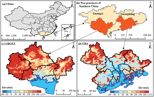
In our study, two coastal urban agglomerations were selected: the Guangxi Beibu Gulf Economic Zone (GBGEZ) and the Guangdong-Hong Kong-Macao Greater Bay Area (GBA). The GBGEZ covers the latitude 20°40’and 24°2’ N, and the longitude 106°33’and 110°53’ E. It includes six cities located in the Guangxi Zhuang Autonomous Region (Figure 1). The GBA covers the latitude 21°25’and 24°23’ N, and the longitude 111°21’and 115°25’ E. It includes 11 cities, with 9 cities in Guangdong Province, Hong Kong, and Macao. The two urban agglomerations are geographically adjacent, and both are in the coastal area of southern China. In addition, considering that some coastal wetlands are distributed outside the coastline, we expanded the study area. According to Ramsar Convention, inland and coastal wetlands are distributed in areas with water depth less than 6 m (Gell, Finlayson, and Davidson 2023). However, due to tidal variation and data errors of water depth, some coastal wetlands (e.g. mangrove, tidal flat) may occur in low tidal level (Wang et al. 2022). Thus, some studies set the threshold of 25 m by trial and error, which could cover all possible wetland extent (Zhang et al. 2022; Zhao and Qin 2020). In this study, we defined the area outside the coastline with a water depth of less than 25 m as the coastal expansion area and implemented wetland classification in both administrative and coastal expansion areas (Figure 1).

Figure 1. The location of our study area. In the figure (c-d), the black polygons denote the administrative boundary, and the blue polygons denote the coastal expansion areas.

2.2. Classification system of wetland ecosystem

Considering the separability of wetland ecosystem types in satellite images, we designed a wetland classification system that is suitable for our study areas based on previous studies (Keith et al. 2023; Liu et al. 2014; Mao et al. 2020). Our classification system included five inland wetlands (inland swamp, marsh, river, lake, and floodplain), three coastal wetlands (mangrove, tidal flat, and coastal shallow water), two human-made wetlands (reservoirs and agricultural ponds). Meanwhile, for better conducting classification, we added six non-wetland types (forest, grassland, built-up land, paddy field, dryland, and bare land) in our classification system. The detailed description of our classification was shown in Table 1.

Table 1. Classification system of wetland ecosystem.

Category I	Category II	Description	sample size
Coastal wetland	Coastal shallow water	Coastal water with depth less than 6 m, including coastal shallow water, bays, straits, etc.	1099
	Mangrove	Woody plant community that grow in coastal tidal flat, distributed in tropical and subtropical climates	533
	Tidal flat	Intertidal zone between high-level tide and low-level tide in coastal areas, including intertidal mudflats, rocks, sands, etc.	728
Human-made wetland	Agricultural pond	Small patchy waterbody with regular shape that used for aquaculture, mostly distributed in coastal areas and nearby rivers.	1695
	Reservoir	Patchy waterbody that artificially constructed for flood regulation and power generation, often equipped with dams.	1049
Inland wetland	Floodplain	Low vegetated areas inundated with seasonal water, including river flooded areas, lake beach, alluvial fan, etc.	258
	Inland swamp	Vegetated wetlands dominated with woody vegetation in inland areas, including forest swamp and shrub swamp	53
	Marsh	Vegetated wetland dominated with herbaceous vegetation	143
	River	Linear waterbody inundated with perennial water	993
	Lake	Nature patchy waterbody inundated with perennial water	88
Non-wetland	Bare land	Areas with low vegetation coverage, including soil, desert, rock, etc.	300
	Built-up land	Artificial construction facilities, including urban land, residential areas, roads, water conservancy facilities, etc.	844
	Dryland	Cropland that relies on natural precipitation, or can be irrigated normally in general years, used for corn, wheat, soybean, etc.	1868
	Forest	Woody vegetation with vegetation coverage greater than 20%, including forest and shrub	3903
	Grassland	Herbaceous vegetation with a coverage of more than 5%, including shrub grassland and sparse forest grassland.	566
	Paddy field	Cropland used for rice, lotus root and other aquatic crops has irrigation facilities, and can be irrigated normally in general years	834

The GBGEZ and GBA located in Southern China, with low altitude. As report by previous studies (Mao et al. 2020; Zhang et al. 2022), there are few coastal marsh (i.e. salt marsh) in these two regions, which is also consistent with our study result. Thus, we do not divide the marsh into inland or coastal.

2.3. Data sources

2.3.1. Landsat-8 image selection and processing

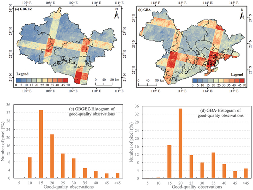
Landsat-8 images were available in the GEE platform. The surface reflectance of Landsat-8 satellite was used in our study. All Landsat-8 images from June 2019 to June 2021 were selected for wetland classification in 2020, with 660 images. To remove cloud contamination in each image, we implemented a mask operation based on the “QA_PIXEL” band of Landsat-8, which could remove cloudy pixels. The remaining pixels of image are good-quality observations. The spatial distributions of good-quality observations are shown in Figure 2(a,b). The pixel values in the two images Figure 2(a,b) represent the number of good observations of Landsat images in corresponding pixel’s location. It was found that good pixels without cloud contaminations could completely covered the study area. We also found that in both GBGEZ and GBA, more than 99.9% of the pixels had more than five good-quality observations, and more than 89% of the pixels had more than 10 good-quality observations Figure 2(c,d).

Figure 2. Image statistics of Landsat-8 time series from June 2019 to June 2021 in our study area. (a-b) are the numbers of spatial distributions of good-quality observation (pixel without could cover) in the GBGEZ and GBA, respectively. (c-d) are histograms of good-quality observations in the GBGEZ and GBA, respectively.

2.3.2. Auxiliary data

In our study, we collected a series of auxiliary datasets that could be divided into six groups: water, tidal flat, mangrove, Land Use/cover Change (LUCC), topographic, and other auxiliary datasets. Detailed descriptions of the datasets are provided in Table 2. These datasets were used for sample production, classification assistance, and data inter-comparison.

Table 2. Auxiliary dataset list in our study.

Category	Name	Spatial resolution	Time period	Data source
Elevation dataset	ETOPO1	1 arc-minute	—	Amante and Eakins (2009)
	Shuttle Radar Topography Mission (SRTM)	30 m	2000	Farr et al. (2007)
LUCC dataset	China Ecosystem-type Classification Dataset (CECD)	5 m	2020	Ouyang et al. (2016)
	China Land Cover Dataset (CLCD)	30 m	1985–2019	Yang and Huang (2021)
Mangrove dataset	Global Mangrove Distribution	30 m	2000	Giri et al. (2011)
	Global Mangrove Watch (GMW)	30 m	1984–2016	Bunting et al. (2018)
	HSL_MangroveChina_LASAC_share	2 m/30 m	1978–2018	Zhang et al. (2020)
	Mangrove Map of China for 2019	10 m	2019	Zhao and Qin (2020)
Open water dataset	Global Surface Water (GSW)	30 m	1984–2020	Pekel et al. (2016)
	HydroLakes	1:100 000	—	Messager et al. (2016)
	Global georeferenced Database of Dams (GOODD)	—	—	Mulligan, van Soesbergen, and Saenz (2020)
	Open Street Map Dam (OSM_Dam)	—	—
Other auxiliary dataset	Global River Widths from Landsat (GRWL)	30 m	—	Allen and Pavelsky (2018)
	Reservoir Point Of Interest (POI)	—	—	Amap open platform (https://lbs.amap.com/)
Tidal flat dataset	Global Intertidal Change	30 m	1990–2017	Murray et al. (2019)
	Tidal Wetlands in East Asia (TEWA)	10 m	2020	Zhang et al. (2022)

The LUCC denote Land Use/cover Change.

For the LUCC dataset, it includes China Ecosystem-type Classification Dataset (CECD) and China Land Cover Dataset (CLCD). The CECD includes 7 wetland sub-types and 14 non-wetland broad types (Table A1), which was produced by visual interpretation based on multiple satellite images (e.g, Gaofen-1, Gaofen-2, Ziyuan-3) in 2020, with overall accuracy over 90%. The CLCD includes nine broad land use types, of which the forest, water, and impervious have high accuracy. For the POI, GOODD and OSM_Dam points, they were used to assist in extracting reservoirs. In addition, it should be noted that the four mangrove datasets for all periods were merged into a potential mangrove extent (PME) to assist mangrove extraction.

3. Methods

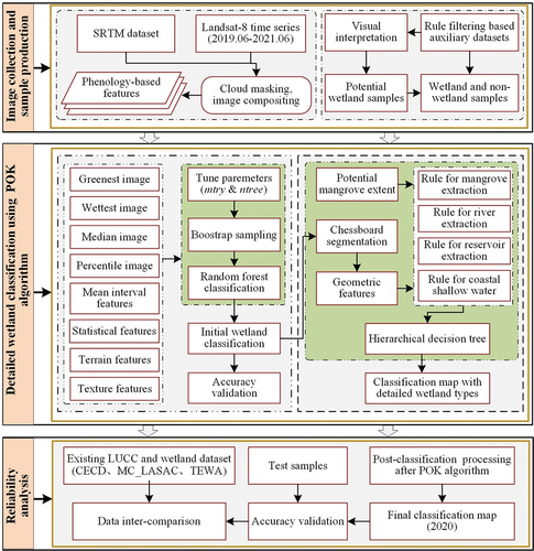
This study developed a new method for detailed wetland type classification in two coastal urban agglomerations, and the process can be divided into three parts: (1) image selection and sample production, (2) detailed classification of wetland types using the POK algorithm, and (3) data inter-comparison based on our test samples and existing datasets. The workflow of this study is shown in Figure 3.

Figure 3. Workflow of detailed wetland type classification. SRTM denote Shuttle Radar Topography Mission, CECD denote China Ecosystem-type classification dataset, MC_LASAC denote HSL_MangroveChina_LASAC_share, TWEA denote tidal wetlands in East Asia.

3.1. Training sample generation

Based on auxiliary datasets, we produced training samples by combining rule filtering and visual interpretation. Our sample generation method was divided into two parts (Table 3): automatic and semiautomatic sample production.

Table 3. Illustration of training sample generation based on rule filtering and visual interpretation.

Category	Auxiliary dataset	Rule filtering	Visual interpretation
Automatic sample production
Built-up land	CLCD	√
Forest	CLCD	√
Lake	CECD, GSW, HydroLake	√
Mangrove	GMW	√
Reservoir	GSW, HydroLake	√
River	GSW, CECD	√
Tidal flat	Global Intertidal Change	√
Semiautomatic sample production
Agricultural pond	CECD	√	√
Bare land	CECD	√	√
Dryland	CECD	√	√
Floodplain	GSW, MODIS	√	√
Grassland	CECD	√	√
Inland swamp	GSW, MODIS	√	√
Marsh	GSW, MODIS	√	√
Paddy field	CECD	√	√

In the GSW dataset, the occurrence layer that recorded the frequency with which water was present from 1984 to 2022 was selected. Its pixel values range from 0 to 100. The MODIS refer to MOD13Q1 product, with NDVI band of 250 m spatial resolution. The MODIS NDVI from 2000 to 2020, available in GEE platform, were selected to construct the NDVI time series.

First, we directly produced samples based on auxiliary datasets. ① For rivers, lakes, and reservoirs, we used GSW, CECD, and HydroLAKES to produce training samples. Based on the GSW data from 1984 to 2020, water points were randomly generated within a water inundation frequency (WIF) larger than 80%. The river and lake samples were then selected using the river and lake extent of CECD dataset. The reservoir samples and some of the lake samples were selected using the reservoir and lake extent of HydroLAKE. ② For mangroves and tidal flats, we used the GMW and Global Intertidal Change data from 2016 to produce their samples. ③ For forest and built-up land, we used the CLCD from 2015 to 2019 to produce random samples. The two land use types in CLCD shared high map accuracy, with F-score over 72%, which could be used to produce reliable samples. To improve sample’s quality, we overlaid the multiyear CLCD to generate stable forest and built-up land regions and then randomly created samples within the intersected regions.

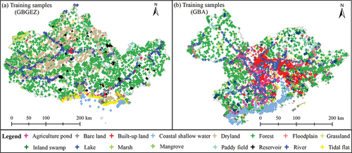
In the second part, we first produced potential samples based on an auxiliary dataset and then visually investigated and corrected them based on very high-resolution (VHR) images of Google Earth platform in 2020. Referring to (Peng et al. 2021, 2023), we produced sample points of floodplain, inland swamp, and marsh by combining GSW, MODIS NDVI time series, and visual interpretation. For agricultural pond, paddy field, dryland, grassland, and bare land classes, we produced samples using the CECD of 2020. We firstly extract their extents using the CECD dataset, and then randomly generated sample points in the corresponding type’s boundary in ArcGIS 10.4 software. Meanwhile, considering the inherent errors of CECD, we manually inspected these samples by visual interpretation, and corrected their attributes if their sample labels were wrong. Finally, through the above process, we produced 14,954 training samples. The sample size of each type was shown in Table 1. The spatial distributions of the training samples are shown in Figure 4.

Figure 4. Spatial distribution of training sample points in the GBGEZ (a) and GBA (b).

3.2. An algorithm of pixel- and object-based with knowledge (POK)

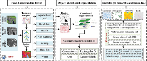
By combining pixel-based random forest and an object-based hierarchical decision tree, we developed a pixel- and object-based algorithm with knowledge (POK). The “pixel” refers to the pixel-based random forest classification (Deng et al. 2023), the “object” refers to polygons with geometric properties segmented by chessboard segmentation, and the “knowledge” refers to the rule set of the hierarchical decision tree. A concept graph of the POK algorithm is shown in Figure 5.

Figure 5. Concept graph of the POK algorithm. GEE denotes the Google Earth Engine. PME denote the potential mangrove extent. POK denotes the pixel- and object-based algorithm with knowledge.

3.2.1. Input features

To capture the seasonal characteristics of wetlands and non-wetlands, we used Landsat-8 images from June 2019 to June 2020 to construct phenology-based features. In addition to six spectral bands (green, blue, red, NIR [Near Infrared], SWIR1 [shortwave Infrared1], and SWIR2 [Shortwave Infrared2]), five spectral indices were chosen, namely, the normalized difference vegetation index (NDVI) (Rouse et al. 1974), enhanced vegetation index (EVI) (Huete et al. 1997), normal difference water index (NDWI) (McFeeters 1996), modified normal difference water index (MNDWI) (Xu 2006), and automated water extraction index (AWEI) (Feyisa et al. 2014). Based on the GEE platform (Gorelick et al. 2017), we composited all bands and indices of two-year images into phenology-based features, including median, wettest, and greenest images with spectral bands, and percentile, mean interval, and statistical features of spectral indexes (Figure 6).

Figure 6. Phenology-based features constructed by the GEE platform.

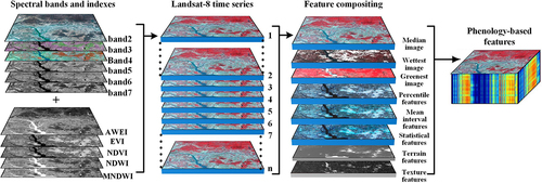
The median image reflect the average reflectance during the study period and was composited using the median() function (Jia et al. 2020). The wettest image represents the maximum extent of permanently inundated water bodies and was composited using qualityMosaic (“MNDWI”) (Jia et al. 2021). The greenest image represents pixels with high levels of greenness across the two-year period and was composited using qualityMosaic (“NDVI”) (Zhang et al. 2022). The percentile features, mean interval features, and statistical features were composited based on the time series of spectral indices (AWEI, EVI, NDVI, NDWI, and MNDWI). Percentile features were calculated at 10%, 25%, 50%, 75%, and 90% using the percentile() function (Murray et al. 2019). Specifically, the histogram of spectral index at a pixel location was calculated based on their two-years’ time series, and then the percentile features were extracted at a certain value (i.e. 10%, 25%, 50%, 75%, 90%) for this pixel (Xie et al. 2019). The mean interval features were calculated at intervals of 0–10%, 10–25%, 25–50%, 50–75%, 75–90%, 90–100%, 10–90%, and 25–75% using the ee.Reducer.intervalMean() function (Wu et al. 2021). Descriptive statistics were calculated, including the maximum, minimum, median, and standard deviation of the time series of spectral indices and were composited using the max(), min(), median(), and stdDev() functions, respectively. Terrain features, including elevation, slope, and aspect, were calculated based on the SRTM dataset. Texture features were calculated using a gray-level co-occurrence matrix based on the median composite NDVI image. Through these operations, we produced 114 feature layers in our phenology-based feature collection.

In addition, to facilitate detailed wetland type classification, we chose four geometric features: compactness, rectangular fit, length/width, and area. The four features were calculated based on chessboard segmentation, which was implemented using eCognition 8.7 software (Zheng et al. 2016). It should be noted that the geometric features were used in object-based hierarchical decision tree, rather than stack them into phenology-based features for pixel-based random forest classification.

3.2.2. Pixel-based random forest classification

Based on phenology-based features, we implemented pixel-based random forest classification using the GEE platform. Random forest (RF) is an ensemble algorithm that can avoid overfitting and is insensitive to feature redundancy. Thus, RF is widely used in wetland and land use mapping (Deng et al. 2023; Mahdianpari et al. 2020; Yang and Huang 2021). The main parameters of the RF were the numbers of randomly selected features (mtry) and decision trees (ntree). mtry is usually set as the square of the total number of input feature layers (Feng et al. 2022). Thus, the mtry value in our study was 11. Considering the mapping accuracy and computational efficiency, we set ntree to 100. In our study, we used the pixel-based RF algorithm to initially extract six wetland types (water, swamp, marsh, floodplain, tidal flat, and agricultural pond) and six non-wetland types (forest, grassland, built-up land, paddy field, dryland, and bare land). Considering the similar climate and geographical environment, we used all the training samples of GBGEZ and GBA to train the RF classifier and generate classification maps simultaneously.

3.2.3. Object-based hierarchical decision tree classification

To separate the six wetland types of the RF classification into detailed types, we designed an object-based hierarchical decision tree by combining geometric features and auxiliary datasets. Geometric features (compactness, rectangular fit, length/width, and area) of water bodies were calculated using chessboard segmentation in eCognition software. Firstly, the waterbody raster with binary values (i.e. water [1] and non-water [0]) was extracted from the classification maps of RF pixel-based algorithm. Secondly, the waterbody vectors were derived from the water raster using the ArcGIS 10.4 software. Thirdly, using the waterbody raster as the input raster and the waterbody vectors as the input vector, the chessboard segmentation was used to calculate compactness, rectangular fit, length/width, and area (Zheng et al. 2016).

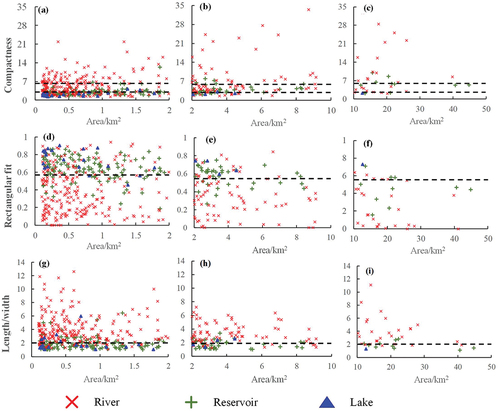
Based on the training samples, we counted the geometric features of the reservoirs, rivers, and lakes (Figure 7). It was found that the river has the largest compactness and length/width and the smallest rectangular fit among the three waterbody types. Based on the above analysis and our trial and error, we found that ① The rule of “Compactness >2.5” extracted 83.0% of rivers, while the extraction results contained 69.1% of reservoirs and 30.8% of lakes. ② The rule of “Rectangular fit <0.55” extracted 75.5% of rivers, while its results contained 25.5% of reservoirs and 3.85% of lakes. ③ The rule of “Length/width >2.0” extracted 86.1% of rivers, while its results contained 32.7% of reservoirs and 26.9% of lakes. Thus, we aggregated the three individual rules to form a consolidated rule set for river extraction, namely, “Compactness >2.5 & Rectangular fit < 0.55 & Length/width >2.0.” In addition, we found that the above rule set may underestimate large rivers, which could be well extracted by the rule of “Compactness >6.0.” In summary, we used the rule set of “Compactness >2.5 & Rectangular fit <0.55 & Length/width >2.0” or “Compactness >6.0” to extract the rivers.

Figure 7. Geometric features of reservoirs, rivers and lakes used in the development of the rule set of hierarchical decision. The three geometric characteristics are shown for three size categories, between 0–2 km², 2–10 km² and 10–50 km² for Compactness (a-c), rectangular fit (d-f) and length/width (g-i), respectively.

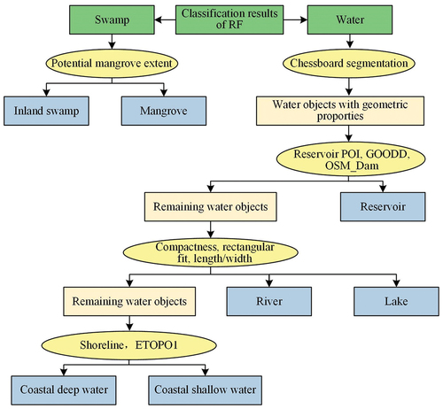
For the reservoirs, we used the reservoir POI, GOODD, and OSM_Dam points to filter them from the water objects. Reference to the study of Mao et al. (2020), we extracted the coastal shallow water using the shoreline and ETOPO1 datasets. Water bodies located outside the shoreline with a depth of less than 6 m were identified as coastal shallow waters. We used the potential mangrove extent (PME) to extract mangroves, and the remaining swamp was labeled as inland swamp. The workflow of the hierarchical decision tree is shown in Figure 8.

Figure 8. Illustration of hierarchical decision tree. The green boxes denote the initial input data, the yellow ovals denote process operations, the light yellow boxes denote the intermediate output, and the light blue denote the final output. In addition, it should be noted that the coastal deep water does not belong to wetlands, which was grouped into background.

3.3. Post-classification processing

In this study, additional steps were used in an attempt to improve the wetland classifications of our POK algorithm. First, waterbodies with areas less than 0.01 km² were selected and then intersected with classified agricultural ponds with a 30 m buffer, which were then labeled as agricultural ponds. Second, agricultural ponds with areas less than 0.01 km² were selected and intersected with classified rivers, which were then labeled as rivers. Third, we used the GRWL dataset to filter them from unclassified water bodies, and the selected polygons were labeled rivers. Fourth, we implemented visual interpretation to identify obvious unclassified water bodies. Subsequently, water bodies with a depth range of 6–25 m were set as the background, and the remaining water bodies were labeled as unclassified water. Finally, we used the majority of the algorithms of the ENVI software to remove small patches of marsh and inland swamps. In the majority algorithm, its kernel size is 5 × 5, and its center pixel weight is 1.0.

3.4. Comparison analysis

3.4.1. Accuracy validation based on test samples

To validate our wetland classification accuracy, we produced test samples by combining stratified random sampling with visual interpretation (Olofsson et al. 2014). Specifically, we first generated random points using stratified random sampling method in ArcGIS 10.4 software, and then implemented visual interpretation for these points by combining Google Earth and Collect Earth platform (Bey et al. 2016). For the visual interpretation, the Google Earth platform offers VHR images, and the Collect Earth platform was used to manage sample points. Finally, 2,034 points were randomly produced. We then chose the overall accuracy (OA), user accuracy (UA), and producer accuracy (PA) to evaluate the accuracy of our wetland map (Stehman et al. 2021). The standard errors of the three indices were also calculated to measure their uncertainties at the 95% confidence level. In addition, we defined accuracy metrics greater than 80%, between 65% and 80%, and less than 65% as high accuracy, medium accuracy, and low accuracy, respectively.

3.4.2. Intra-comparisons with existing datasets

To further check the accuracy of our wetland maps, we compared them with existing datasets, including the CECD, MC_LASAC, and TWEA datasets. We calculated the areas of individual types in different maps and calculated the areas of spatial consistency by overlay analysis.

The CECD dataset, acquired from the Ministry of Ecology and Environment of China, was produced at a spatial resolution of 5 m by visual interpretation, with 7 wetland types and 14 non-wetland types (Table A1). This dataset was used to test the overall consistency of the maps. Because the CECD merged the reservoirs and agricultural ponds into one type (reservoir/pond), we merge these two classes of our wetland maps into one class, and compared it with CECD dataset. Meanwhile, because the coastal shallow waters and tidal flats of the CECD were not complete in the GBA but were relatively complete in the GBGEZ, we only compared the tidal flats in the GBGEZ. In addition, we aggregated the 19 non-wetland types into 6 types to match our classification system. The corresponding relationship between the classes of CECD and our wetland classification was shown in Table A1.

The MC_LASAC mangrove dataset of 2018, with a 2 m spatial resolution and an OA of 98%, was used to check the accuracy of our predicted extent of mangroves. The TWEA tidal flat of 2020, at a spatial resolution of 10 m, with both UA and PA greater than 94%, was used to test the accuracy of our predicted extent of tidal flats. In our study, we implemented data inter-comparison in ArcGIS 10.4 software. All datasets were projected into WGS_1984_Albers coordinate system.

4. Results

4.1. Classification results of pixel-based RF algorithm

Based on phenology-based features, we used a pixel-based RF algorithm to extract six wetland types and six non-wetland types. Their spatial distributions are shown in Figure 9. The accuracy validation indicated that the OA of the wetland map was 91.8%±1.2% (Table 4). For wetland types, the water and tidal flats had the highest accuracy, with UA and PA values over 92.2%. The swamp, floodplain, and agricultural ponds also had high accuracy, with UA and PA values over 88.0%. The marsh had low accuracy with a low PA, indicating that some omission errors existed. The reason was that the small marshes were spectrally confused with other types, such as dryland, swamp and paddy field. For non-wetland types, forest and built-up land had the highest accuracy, with UA and PA values over 91.2%. The dryland also achieved high accuracy, with UA and PA values over 83.3%. Grassland, paddy field, and bare land had moderate accuracy, with most UA and PA values over 72.0%.

Figure 9. Spatial distribution of six wetland types and six non-wetland types.

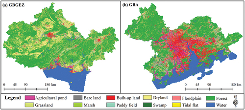
Table 4. Accuracy results of the pixel-based RF classifications.

OA	91.8%±1.2%
Individual accuracy metric	UA	PA
Agricultural pond	89.1% ± 8.3%	89.2% ± 7.8%
Bare land	92.3% ± 8.5%	72.0% ± 12.6%
Built-up land	91.2% ± 4.6%	97.8% ± 2.4%
Dryland	83.3% ± 3.9%	89.0% ± 3.4%
Floodplain	89.8% ± 8.6%	88.0% ± 9.1%
Forest	97.0% ± 1.1%	96.9% ± 0.9%
Grassland	75.0% ± 12.9%	66.0% ± 13.3%
Marsh	100.0% ± 0.0%	16.1% ± 12.0%
Paddy field	75.8% ± 10.4%	76.9% ± 10.3%
Swamp	89.1% ± 7.7%	95.0% ± 5.6%
Tidal flat	94.2% ± 6.4%	98.0% ± 3.9%
Water	92.2% ± 3.6%	96.7% ± 2.4%

4.2. Detailed wetland type classification results

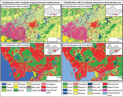
We used an object-based hierarchical decision tree to further divide the six wetland types into 10 wetland types (Figure 10). Specifically, we divided the water into rivers, lakes, reservoirs and coastal shallow water, and divided the swamps into inland swamp and mangrove. Finally, there were 10 wetland types in our study. The spatial comparison between before and after fine classification in two typical regions was shown in Figure 11.

Figure 10. Spatial distribution of 10 wetland types in 2020.

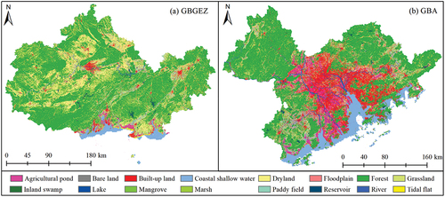
Figure 11. The spatial comparison between before and after fine classification in two typical regions. The (a) and (c) were classifications with 6 wetlands using pixel-based random forest, and the (b) and (d) were classifications with 10 wetlands using object-based hierarchical decision tree. The (a)-(b) were a typical region in GBGEZ, and the (c)-(d) are typical region in GBA.

The accuracy validation indicated that the OA of our wetland map was 91.6%±1.2% (Table 5). For inland wetlands, rivers and floodplains had high accuracy, with UA and PA values over 88.0%. Lakes had moderate accuracy, with a UA and PA of >72.2%. The inland swamps and marshes had low accuracy because they were difficult to extract owing to their very small areas. For coastal wetlands, all three categories achieved good accuracy, with UA and PA exceeding 90.7%. For human-made wetlands, reservoirs had the highest accuracy, with UA and PA values over 90.7%. Agricultural ponds also achieved good accuracy, with a UA and PA of >88.1%.

Table 5. Accuracy results of hierarchical decision tree classification.

Category I	Category II	UA	PA
Coastal wetland	Coastal shallow water	97.7% ± 3.2%	95.5% ± 4.3%
	Mangrove	90.7% ± 7.8%	98.0% ± 3.9%
	Tidal flat	94.2% ± 6.4%	98.0% ± 3.9%
Human-made wetland	Agriculture pond	88.1% ± 8.3%	94.5% ± 6.1%
	Reservoir	90.7% ± 7.8%	98.0% ± 3.9%
Inland wetland	Floodplain	89.8% ± 8.6%	88.0% ± 9.1%
	Inland swamp	50.0% ± 43.8%	30.0% ± 29.9%
	Lake	76.5% ± 20.8%	72.2% ± 21.3%
	Marsh	100.0% ± 0.0%	16.2% ± 12.0%
	River	90.6% ± 7.9%	96.0% ± 5.5%
Non-wetland	Bare land	92.3% ± 8.5%	72.0% ± 12.6%
	Built-up land	91.3% ± 4.6%	97.8% ± 2.4%
	Dryland	83.2% ± 3.9%	89.6% ± 3.3%
	Forest	96.9% ± 1.1%	97.2%±1.0%
	Grassland	75.0% ± 12.9%	66.0% ± 13.3%
	Paddy field	75.8% ± 10.4%	76.9% ± 10.3%
OA	91.6% ± 1.2%

For non-wetlands, forests and built-up lands had the highest accuracy, with UA and PA values over 91.3%. The drylands also achieved high accuracy, with a UA and PA of over 83.2%. Grasslands, paddy fields, and bare lands had moderate accuracy, with most accuracy indices exceeding 0.72. In summary, we believe that our wetland map achieved a high accuracy.

4.3. Intra-comparison with existing datasets

4.3.1. Comparison with the CECD land use dataset

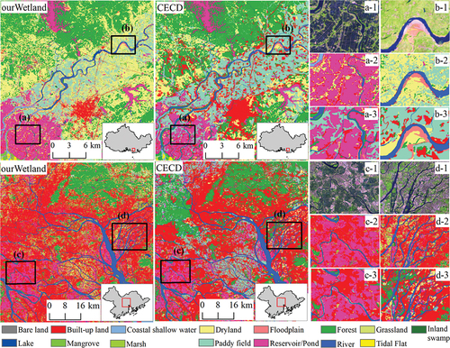
A spatial comparison between the CECD and our maps in two large typical regions is shown in Figure 12. It was found that the land-use types in the two datasets shared similar spatial distributions. The agricultural ponds in our wetland map had a distribution similar to that of the CECD Figure 12(a-c). The rivers in our wetland map were accurately extracted and consistent with the CECD dataset Figure 12(d). For the paddy fields and drylands, there were some inconsistencies, but the cropland combined with paddy fields and drylands had good spatial consistency in the two datasets Figure 12(b).

Figure 12. Intra-comparison between our wetland maps and the CECD dataset. ourWetland refers to our wetland map.

To quantify the consistency and divergence between our wetland classifications and CECD dataset, we calculated the confusion matrix between wetlands and non-wetland types in GBGEZ (Table 6) and GBA (Table 7). The results indicated that the spatial consistency of all land use types accounted for 84.9% and 74.6% of GBGEZ and GBA, respectively.

Table 6. Confusion matrix between our wetland and CECD dataset in GBGEZ. The unit is percentage (%). In this table, the diagonal values represent the percentage of consistency, while others represent the difference between two datasets.

	CDCD dataset
Our Wetland Classifications		La	Riv	FP	TF	CSW	RP	Ft	GL	BUL	PF	DL	BL
	La	0.1	10.1	0.2	0.0	0.0	72.7	5.0	0.0	2.1	4.4	5.4	0.0
	Riv	0.1	80.4	2.1	0.1	0.1	3.4	6.2	0.1	1.1	2.6	3.9	0.0
	FP	0.1	9.9	3.4	1.3	1.1	24.6	6.4	0.4	31.1	6.1	15.4	0.3
	TF	0.0	4.0	0.4	67.4	24.6	0.9	1.3	0.1	1.1	0.2	0.0	0.0
	CSW	0.0	12.5	0.1	26.1	60.2	0.6	0.2	0.0	0.3	0.0	0.0	0.0
	RP	0.2	7.6	0.8	2.7	2.5	64.6	8.6	0.2	4.2	5.5	2.9	0.0
	Ft	0.0	0.4	0.0	0.0	0.0	0.4	86.4	0.2	0.9	4.4	7.3	0.0
	GL	0.0	0.5	0.1	0.0	0.0	0.4	64.3	0.5	7.9	11.1	15.1	0.1
	BUL	0.0	1.2	0.2	0.3	0.2	3.9	6.4	0.4	77.1	5.5	4.5	0.2
	PF	0.0	1.3	0.2	0.0	0.0	1.3	10.5	0.2	8.0	63.1	15.5	0.0
	DL	0.0	1.2	0.1	0.0	0.0	1.4	22.7	0.2	10.5	24.8	39.1	0.0
	BL	0.0	0.2	0.2	0.1	0.1	1.3	15.8	0.4	67.0	4.7	9.8	0.4

La->Lake, Riv->River, TF->Tidal flat, CSW->Coastal shallow water, RP->Reservoir/Pond, Ft->Forest, GL->Grassland, BUL->Built-up land, PF->Paddy field, Dryland->DL, BL->Bare land.

Table 7. Confusion matrix between our wetland and CECD dataset in GBA. The unit, meanings of elements, and abbreviations are same as Table 6.

	CDCD dataset
Our Wetland Classifications		La	Riv	FP	TF	CSW	RP	Ft	GL	BUL	PF	DL	BL
	La	5.0	1.1	0.4	—	—	79.0	8.3	0.2	3.2	1.5	1.2	0.0
	Riv	0.2	87.0	1.1	—	—	3.6	3.1	0.6	2.8	1.1	0.6	0.0
	FP	8.6	9.8	6.9	—	—	31.5	7.3	1.7	21.6	8.7	3.0	0.8
	TF	—	—	—	—	—	—	—	—	—	—	—	—
	CSW	—	—	—	—	—	—	—	—	—	—	—	—
	RP	1.2	5.0	0.3	—	—	68.7	5.3	0.7	9.1	7.5	2.2	0.0
	Ft	0.0	0.3	0.0	—	—	0.9	93.7	0.1	1.2	2.0	1.8	0.0
	GL	0.0	0.7	0.2	—	—	2.1	59.2	2.5	12.9	13.7	8.0	0.7
	BUL	0.0	1.0	0.1	—	—	5.0	9.4	0.9	76.2	4.7	2.5	0.2
	PF	0.0	1.6	0.4	—	—	4.3	17.1	0.9	8.8	54.2	12.6	0.1
	DL	0.0	1.7	0.3	—	—	5.3	31.6	1.3	18.9	27.9	12.8	0.2
	BL	0.2	0.3	0.3	—	—	3.0	15.2	1.3	68.7	4.1	4.5	2.4

For individual wetlands, the river had highest spatial consistency, which accounted for 80.4% and 87.0% of our river in GBGEZ and GBA, respectively. The tidal flat, coastal shallow water, and reservoir/pond have moderate spatial consistency. In GBGEZ, the spatial consistency of four wetland types accounted for 67.4%, 60.2%, and 64.6% of the corresponding types of our wetlands, respectively. In GBA, the reservoir/pond accounted for 68.7% of that of our wetlands. For individual non-wetlands, the forest had the highest spatial consistency, which accounted for 86.4% and 93.7% of our forest in GBGEZ and GBA, respectively. The built-up land and cropland (including paddy field and dryland) had moderate spatial consistency, of which most of their percentage exceeded 65%. In summary, it was found that categories with large areas had high spatial consistency, while rare land use types had low spatial consistency.

In addition, although our wetland classification has high spatial consistency with CECD, there were still divergences between these two datasets. The reasons mainly involved three aspects. First, the production method of datasets resulted in different regularities of land use shapes. For the CECD, it was produced by manual digitizing. If there were small land use patches within a large land use patch, these small patches were merged with the large patch. In contrast, the small land use patches were accurately extracted from our wetland maps, and they would not be merged into the large land patches. Second, our wetland classifications also had classification errors. For example, the mapping accuracies of small land use types were relative low. The paddy field and dryland had some misclassifications due to their spectral similarity. Third, for some land use types, their definitions were different in the two classification systems. For example, the CECD did not separate the agricultural ponds and reservoir, and the reservoir/pond of CECD did not completely include agricultural ponds.

4.3.2. Comparison with mangrove dataset

The statistical results indicated that the mangrove areas of the two datasets were similar, with our mangrove area being 122.5 km² and the MC_LASAC mangrove area being 116.9 km². Their spatial consistency had an area of 90.8 km², accounting for 74.1% of our mangrove area. In addition, four typical regions were chosen to further examine spatial details (Figure 13). The two mangrove datasets shared an almost identical spatial distribution and extent.

Figure 13. Intra-comparison between the MC_LASAC dataset and our mangrove. The first row shows the mangrove distribution of our wetland map in GBGEZ and GBA, respectively.

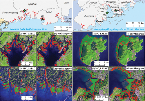
For the divergence between the two mangrove datasets, it was mainly resulted from classification methods and data sources. In our study, we extracted the mangrove using the POK algorithm based on Landsat images. In contrast, the MC_LASAC of 2018 was mapped by combining object-based image analysis and interpreter editing based on 2-m resolution Gaofen-1 and Ziyuan-3 satellite imagery. Compared with our mangrove, the patches of MC_LASAC mangrove were more refined and regular.

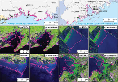
4.3.3. Comparison with tidal flat dataset

The statistical results indicated that our tidal flat area was 349.2 km², whereas the tidal flat area of the TWEA was 643.8 km². Their spatial consistency had an area of 278.8 km², which accounted for 78.8% of our tidal flat. Our tidal flat area was smaller than that of the TWEA dataset. These differences mainly resulted from tidal variation. The TWEA was produced by capturing the high tidal images and low tidal images based on the Sentinel-2 time series and delineated the maximum extent of the tidal flat at a low level. Our phenology-based features characterized the average tidal level and could not capture the low tidal level well. Thus, our wetland maps may underestimate the tidal flats in the GBGZA and GBA. However, the two tidal flats have similar spatial distributions. As shown in Figure 14, the spatial extent of the TWEA was larger than that of our study, while their spatial distributions were similar.

Figure 14. Intra-comparison between the TWEA dataset and our tidal flat. The first row shows the spatial distribution of the tidal flat in our wetland map.

4.4. Area analysis of wetlands in two urban agglomerations

Based on our POK algorithm and Landsat-8 time series, we produced wetland maps with 10 wetland types and 6 non-wetland types in the GBGEZ and GBA. The area statistics of wetlands and non-wetlands in the two coastal urban agglomerations are shown in Table 8.

Table 8. Areas of wetland types and non-wetland types in two urban agglomerations (unit: km²).

Category I	Category II	GBGEZ	GBA
Coastal wetland	Coastal shallow water	1975.3	5078.8
	Mangrove	81.7	40.9
	Tidal flat	278.7	70.4
Human-made wetland	Agricultural pond	697.8	3654.3
	Reservoir	498.9	445.0
Inland wetland	Inland swamp	18.9	110.2
	Marsh	33.0	109.2
	Lake	50.5	70.4
	River	505.7	1234.1
	Floodplain	58.3	118.8
Non-wetland	Bare land	592.8	645.7
	Built-up land	2010.8	8962.1
	Dryland	19449.7	6466.1
	Forest	44859.4	29928.5
	Grassland	1275.0	725.1
	Paddy field	2282.2	2916.6

The wetland area of the GBGEZ in 2020 was 4198.8 km², of which the areas of inland wetlands, coastal wetlands and human-made wetlands were 666.4 km², 2335.7 km², and 1196.7 km², respectively. The three wetlands of categories I accounted for 15.9%, 47.5%, and 37.5% of total wetland area of GBGEZ, respectively. Among individual wetlands, the coastal shallow waters had the largest area, followed by agricultural ponds, rivers, reservoirs, tidal flats, mangroves,floodplains, lakes, marshes, and inland swamps. For inland wetlands, rivers had the largest area, with an area of 505.7 km². For coastal wetlands, areas of mangrove, tidal flat and coastal shallow water were 81.7 km², 278.7 km², and 1975.4 km², respectively. For human-made wetlands, reservoirs, and agricultural ponds had an area of 498.8 km² and 697.8 km², respectively.

Compared with the GBGEZ, the GBA had larger wetland areas with a value of 10,932.2 km², of which the inland wetland area, coastal wetland area, and human-made wetland area were 1642.7 km², 5190.1 km² and 4099.3 km², respectively. The three wetlands of categories I accounted for 15.9%, 47.5%, and 37.5% of total wetland area of GBA, respectively. For inland wetlands, rivers had the largest area with a value of 1234.1 km². For coastal wetlands, areas of mangroves, tidal flat and coastal shallow water were 40.9 km², 70.4 km², and 5078.8 km², respectively. Human-made wetlands, reservoirs, and agricultural ponds had an area of 445.0 km² and 3654.4 km², respectively.

5. Discussion

5.1. Effectiveness of our POK algorithm

Wetland mapping can offer useful information for wetland management and protection, which can well serve in the Convention on Biological Diversity and support the Global Biodiversity Framework (Fitoka et al. 2020; van Rees et al. 2021). Wetland classification methods can be grouped into two categories: supervised classification and hierarchical decision trees. Supervised classification methods can effectively extract rough land use types (Piaser and Villa 2023; Xu et al. 2022) but are not suitable for detailed wetland-type classification. For example, supervised classification can extract water bodies well but cannot identify water cover types (e.g. rivers, lakes, reservoirs) (Li and Niu 2022). The hierarchical decision tree method can effectively realize detailed wetland-type classification by combining spectral and geometric features. However, its rules and thresholds always change over time and regions (Fitoka et al. 2020). The complexity of the algorithm limits its wide application in wetland classification.

In our study, we developed a novel algorithm for detailed wetland classification. Our POK algorithm was accurate, effective, and robust for detailed wetland classification. In our POK algorithm, the pixel-based RF was used to extract 6 wetland types (Table 4), and the object-based hierarchical decision tree was used to divide the above wetlands into 10 wetland types (Table 5). Compared with traditional supervised classification, the POK algorithm can well distinguish wetland types with similar spectra, such as lakes, rivers, and reservoirs. Compared with the object-based decision tree algorithm, the POK algorithm exhibited better generalization. Its classification rules and thresholds will not change over time and regions. Meanwhile, the POK algorithm utilized the phenology-based features that could capture the spectral and seasonal characteristics of wetlands well (Wu et al. 2021), which well assisted in the classification of complex wetland types.

The accuracy validation results indicated that the OA of our wetland map was 91.8%±1.2%. For wetland types, most had UA and PA values greater than 88.0%. For the non-wetland types, the UA and PA values were over 72.0%. The above accuracy indices show that our wetland map had high accuracy. To further test the accuracy of our map, we implemented a cross comparison with existing datasets. It was found that the spatial consistencies between our map and CECD accounted for 84.9% and 74.6% in GBGEZ and GBA, respectively. The spatial consistency between our mangrove and MC_LASAC accounted for 74.1% of our mangroves, and the spatial consistency between our tidal flat and TWEA accounted for 78.8% of our tidal flats. Based on above analysis, we believe that our wetland map could reliably reflect the wetland extents in our study areas.

5.2. Limitations, uncertainties, and outlooks

In this study, we successfully mapped 10 wetland types and 6 non-wetland types with high accuracy. However, there are uncertainties and limitations. First, tidal flats were underestimated in the wetland map of our POK algorithm. Our phenology-based features represent the overall status of wetland conditions but do not capture high and low tides (Jia et al. 2021). Second, the accuracy of inland swamps and marshes was low because of their very small areas. The effectiveness of our algorithm for large inland swamps and marsh extraction needs to be further explored in other regions. Third, there were misclassifications between paddy fields and drylands due to sample uncertainties caused by interpretation confusion between paddy fields and drylands and their spectral similarity. Forth, we just determined the value of ntree based on literature review. However, for this parameter, it needed conduct experiments on relationship between ntree and out of bag (OBB) errors. Fifth, we use the ETOPO1 to assist the extraction of coastal shallow water, which may lead to classification errors, because the ETOPO1 was static water depth data with rough spatial resolution.

For our POK algorithm, there are some addition limitations and potential factors affecting our wetland classification. As is known, wetland extents often changes with seasons. Our study did not consider the seasonal variations on wetland changes, which may resulted in errors in mapping wetland extents (Xu, Niu, and Tang 2018). Due to the spectral complexity of wetlands, spectral confusion of wetland types was another factor influencing our classification accuracy. For example, the marsh and inland swamp may misclassify with forest and paddy field (Mahdianpari et al. 2020). In addition, the quality of training samples also affected our POK algorithm. For our training samples, the error of wetland datasets and roughness of manual interpretation may lead to sample errors, which further affected the classification accuracy (Peng et al. 2023).

In future studies, satellite images with high spatial and temporal resolutions should be used to improve wetland classifications, such as Sentinel-2, Gaofen 1–2, and IKONOS. The applicability and accuracy of our POK algorithm when applied to these images require further investigation. Previous studies have indicated that SAR images are beneficial to wetland classification (Feng et al. 2022; Fu et al. 2017) because they can capture valuable information about the water and ground conditions under vegetation canopies. Compared to using optical images alone, combining optical images with SAR will improve the wetland classification (Lu and Wang 2021). However, using SAR images alone for wetland classification is inferior in accuracy compared to utilizing optical image time series (Vanderhoof et al. 2023), because the optical images, with multi-spectral bands, spectral bands, and phenology-based features, can provide more valuable information to the classification algorithm. In addition, to further enhance the application of our study, it is necessary to implement long-term wetland classification and monitor wetland dynamics using our POK algorithm, which could reveal the spatiotemporal evolution of detailed wetland types and offer useful information and knowledge for wetland resource protection and future policy-making.

6. Conclusion

In this study, we developed a POK algorithm for detailed wetland classification by combining a pixel-based random forest algorithm and an object-based hierarchical decision tree. The results indicated that the OA of our wetland map with 10 wetland types was 91.6%±1.2%. Seven wetland types resulted in high accuracies in our POK classification, including rivers, floodplains, mangroves, tidal flats, coastal shallow waters, reservoirs, and agricultural ponds, with UA and PA values over 88.0%. For non-wetland types, most UA and PA values were over 72.0%. By comparing with existing datasets, it was found that the spatial consistency between our wetlands and CECD accounted for 84.9% and 74.6% of GBGEZ and GBA, respectively. For the MC_LASAC and TWEA dataset, our mangroves and tidal flats had 74.1% and 78.8% spatial consistency with corresponding datasets.

In the GBGEZ in 2020, the wetland area was 4,198.8 km², of which the inland wetland area was 666.4 km² (15.9%), the coastal wetland area was 2,335.7 km² (47.5%), and the human-made wetland area was 1,196.7 km² (37.5%). In the GBA in 2020, the wetland area was 10,932.2 km², of which the inland wetland area was 1,642.7 km² (15.9%), the coastal wetland area was 5,190.1 km² (47.5%), and the human-made wetland area was 4,099.3 km² (37.5%). Our study successfully mapped detailed wetland types at a 30 m resolution in two urban agglomerations, which could potentially inform decision-making and planning.

Disclosure statement

No potential conflict of interest was reported by the author(s).

Data availability statement

Table

China Ecosystem-type Classification Dataset (CECD)	The data are not publicly available because its production cost is high, which just available to specific users and departments
China Land Cover Dataset (CLCD)	https://doi.org/10.5281/zenodo.4417810
ETOPO1	https://earthengine.google.com/
Global Mangrove Distribution	https://earthengine.google.com/
Global Mangrove Watch (GMW)	https://data.unep-wcmc.org/datasets/45
Global Intertidal Change	https://earthengine.google.com
Global River Widths from Landsat (GRWL)	https://zenodo.org/record/1297434#.ZCboFHZByUk
Global Surface Water (GSW)	https://earthengine.google.com
GOODD	https://www.globaldamwatch.org/directory
Tidal Wetlands in East Asia (TEWA)	https://figshare.com/articles/dataset/Fujian_zip/14331785
HSL_MangroveChina_LASAC_share	http://www.sasclouds.com/chinese/home/
HydroLakes	https://www.hydrosheds.org/products/hydrolakes
Mangrove Map of China for 2019	https://doi.org/10.11922/sciencedb.00245
Open Street Map Dam (OSM_Dam)	https://www.globaldamwatch.org/directory
Reservoir Point Of Interest (POI)	https://lbs.amap.com/
Shuttle Radar Topography Mission (SRTM)	https://earthengine.google.com/

Additional information

Funding

This work was supported by the National Natural Science Foundation of China under grant numbers U1901219, U21A2022, 42301413, 42071393, and 41971306 and the Natural Science Foundation of Tianjin under grant number 22JCQNJC01420.

Appendix

Table A1. The corresponding relationship between the classes of CECD dataset and our wetland classification.

Classification system of CECD		Classification system of our study
Category I	Category II	Category
Wetland	River	River
	Lake	Lake
	Reservoir/pond	Reservoir, Agricultural pond
	Tidal flat	Tidal flat
	Floodplain	Floodplain
	Coastal shallow water	Coastal shallow water
	Vegetated wetland	Inland swamp, marsh, mangrove
Forest	Forestland	Forest
	Shrub land
	Sparse woodland
	Other forest land
Grassland	High vegetation cover grassland	Grassland
	Median vegetation cover grassland
	Low vegetation cover grassland
Built-up land	Urban land	Built-up land
	Rural Settlement
	Other construction land
Cropland	Paddy field	Paddy field
	Dryland	Dryland
Unused land	Sand land	Bare land
	Saline-Alkali Land
	Bare soil
	Bare rock
	Other

References

- Allen, G. H., and T. M. Pavelsky. 2018. “Global Extent of Rivers and Streams.” Science 361 (6402): 585–25. https://doi.org/10.1126/science.aat0636.
- Amante, C., and B. W. Eakins. 2009. “ETOPO1 arc-minute global relief model: procedures, data sources and analysis.” NOAA Technical Memorandum NESDIS NGDC-24 19 (3): 2009. https://repository.library.noaa.gov/view/noaa/1163
- Bey, A., A. Sánchez-Paus Díaz, D. Maniatis, G. Marchi, D. Mollicone, S. Ricci, J. F. Bastin, et al. 2016. “Collect Earth: Land Use and Land Cover Assessment Through Augmented Visual Interpretation.” Remote Sensing 8 (10): 807.
- Bhatt, P., and A. L. Maclean. 2023. “Comparison of High-Resolution NAIP and Unmanned Aerial Vehicle (UAV) Imagery for Natural Vegetation Communities Classification Using Machine Learning Approaches.” GIScience & Remote Sensing 60:1. https://doi.org/10.1080/15481603.2023.2177448.
- Bon, G., E. Turak, D. Dudgeon, B. Bendandi, M. Thieme, J. Lento, M. Simpson, and FWBON. 2022. Inland Waters in the Post-2020 Global Biodiversity Framework. https://geobon.org/science-briefs/.
- Bunting, P., A. Rosenqvist, R. M. Lucas, L. M. Rebelo, L. Hilarides, N. Thomas, A. Hardy, T. Itoh, M. Shimada, and C. M. Finlayson. 2018. “The Global Mangrove WatchA New 2010 Global Baseline of Mangrove Extent.” Remote Sensing 10 (10). https://doi.org/10.3390/rs10101669.
- Cao, X. S., S. S. Ouyang, W. Y. Yang, Y. Luo, B. C. Li, and D. Liu. 2019. “Transport Accessibility and Spatial Connections of Cities in the Guangdong-Hong Kong-Macao Greater Bay Area.” Chinese Geographical Science 29 (5): 820–833. https://doi.org/10.1007/s11769-019-1034-2.
- Chen, K. X., P. F. Cong, L. M. Qu, S. X. Liang, and Z. C. Sun. 2022. “Annual Variation of the Landscape Pattern in the Liao River Delta Wetland from 1976 to 2020.” Ocean & Coastal Management 224. https://doi.org/10.1016/j.ocecoaman.2022.106175.
- Deng, Y. W., W. G. Jiang, Z. F. Wu, Z. Y. Ling, K. F. Peng, and Y. Deng. 2022. “Assessing Surface Water Losses and Gains Under Rapid Urbanization for SDG 6.6. 1 Using Long-Term Landsat Imagery in the Guangdong-Hong Kong-Macao Greater Bay Area, China.” Remote Sensing 14 (4): 881.
- Deng, Y., Z. F. Shao, C. Y. Dang, X. Huang, W. F. Wu, Q. W. Zhuang, and Q. Ding. 2023. “Assessing Urban Wetlands Dynamics in Wuhan and Nanchang, China.” Science of the Total Environment 901:165777. https://doi.org/10.1016/j.scitotenv.2023.165777.
- Elmahdy, S. I., and M. M. Mohamed. 2018. “Monitoring and Analysing the Emirate of Dubai’s Land Use/Land Cover Changes: An Integrated, Low-Cost Remote Sensing Approach.” International Journal of Digital Earth 11 (11): 1132–1150. https://doi.org/10.1080/17538947.2017.1379563.
- Farr, T. G., P. A. Rosen, E. Caro, R. Crippen, R. Duren, S. Hensley, M. Kobrick, et al. 2007. “The Shuttle Radar Topography Mission.” Reviews of Geophysics 45 (2). https://doi.org/10.1029/2005RG000183.
- Feng, K. D., D. H. Mao, Z. Q. Qiu, Y. X. Zhao, and Z. M. Wang. 2022. “Can Time-Series Sentinel Images Be Used to Properly Identify Wetland Plant Communities?” GIScience & Remote Sensing 59 (1): 2202–2216.
- Feyisa, G. L., H. Meilby, R. Fensholt, and S. R. Proud. 2014. “Automated Water Extraction Index: A New Technique for Surface Water Mapping Using Landsat Imagery.” Remote Sensing of Environment 140:23–35. https://doi.org/10.1016/j.rse.2013.08.029.
- Fitoka, E., M. Tompoulidou, L. Hatziiordanou, A. Apostolakis, R. Hofer, K. Weise, and C. Ververis. 2020. “Water-Related ecosystems’ Mapping and Assessment Based on Remote Sensing Techniques and Geospatial Analysis: The SWOS National Service Case of the Greek Ramsar Sites and Their Catchments.” Remote Sensing of Environment 245. https://doi.org/10.1016/j.rse.2020.111795.
- Fu, B. L., Y. Q. Wang, A. Campbell, Y. Li, B. Zhang, S. B. Yin, Z. F. Xing, and X. M. Jin. 2017. “Comparison of Object-Based and Pixel-Based Random Forest Algorithm for Wetland Vegetation Mapping Using High Spatial Resolution GF-1 and SAR Data.” Ecological Indicators 73:105–117. https://doi.org/10.1016/j.ecolind.2016.09.029.
- Gell, P. A., C. M. Finlayson, N. C. Davidson. 2023. “An Introduction to the Ramsar Convention on Wetlands.” In Ramsar Wetlands, 1–36. Switzerland: Elsevier.
- Giri, C., E. Ochieng, L. L. Tieszen, Z. Zhu, A. Singh, T. Loveland, J. Masek, and N. Duke. 2011. “Status and Distribution of Mangrove Forests of the World Using Earth Observation Satellite Data.” Global Ecology & Biogeography 20 (1): 154–159. https://doi.org/10.1111/j.1466-8238.2010.00584.x.
- Gong, P., H. Liu, M. N. Zhang, C. C. Li, J. Wang, H. B. Huang, N. Clinton, et al. 2019. “Stable Classification with Limited Sample: Transferring a 30-M Resolution Sample Set Collected in 2015 to Mapping 10-M Resolution Global Land Cover in 2017.” Science Bulletin 64 (6): 370–373. https://doi.org/10.1016/j.scib.2019.03.002.
- Gorelick, N., M. Hancher, M. Dixon, S. Ilyushchenko, D. Thau, and R. Moore. 2017. “Google Earth Engine: Planetary-Scale Geospatial Analysis for Everyone.” Remote Sensing of Environment 202:18–27. https://doi.org/10.1016/j.rse.2017.06.031.
- Guo, H. J., Y. P. Cai, Z. F. Yang, Z. C. Zhu, and Y. R. Ouyang. 2021. “Dynamic Simulation of Coastal Wetlands for Guangdong-Hong Kong-Macao Greater Bay Area Based on Multi-Temporal Landsat Images and FLUS Model.” Ecological Indicators 125. https://doi.org/10.1016/j.ecolind.2021.107559
- Hou, T. T., W. W. Sun, C. Chen, G. Yang, X. C. Meng, and J. T. Peng. 2022. “Marine Floating Raft Aquaculture Extraction of Hyperspectral Remote Sensing Images Based Decision Tree Algorithm.” International Journal of Applied Earth Observation and Geoinformation 111:102846. https://doi.org/10.1016/j.jag.2022.102846.
- Huete, A., H. Liu, K. Batchily, and W. Van Leeuwen. 1997. “A Comparison of Vegetation Indices Over a Global Set of TM Images for EOS-MODIS.” Remote Sensing of Environment 59 (3): 440–451.
- Hu, X. D., P. L. Zhang, Q. Zhang, and J. Q. Wang. 2021. “Improving Wetland Cover Classification Using Artificial Neural Networks with Ensemble Techniques.” GIScience & Remote Sensing 58 (4): 603–623.
- Jamali, A., M. Mahdianpari, B. Brisco, J. Granger, F. Mohammadimanesh, and B. Salehi. 2021. “Deep Forest Classifier for Wetland Mapping Using the Combination of Sentinel-1 and Sentinel-2 Data.” GIScience & Remote Sensing 58 (7): 1072–1089. https://doi.org/10.1080/15481603.2021.1965399.
- Jia, M. M., D. H. Mao, Z. M. Wang, C. Y. Ren, Q. D. Zhu, X. C. Li, and Y. Z. Zhang. 2020. “Tracking Long-Term Floodplain Wetland Changes: A Case Study in the China Side of the Amur River Basin.” International Journal of Applied Earth Observation and Geoinformation 92:102185. https://doi.org/10.1016/j.jag.2020.102185.
- Jia, M. M., Z. M. Wang, D. H. Mao, C. Y. Ren, K. S. Song, C. P. Zhao, C. Wang, X. M. Xiao, and Y. Q. Wang. 2023. “Mapping Global Distribution of Mangrove Forests at 10-M Resolution.” Science Bulletin 68:1306–1316. https://doi.org/10.1016/j.scib.2023.05.004.
- Jia, M. M., Z. M. Wang, D. H. Mao, C. Y. Ren, C. Wang, and Y. Q. Wang. 2021. “Rapid, Robust, and Automated Mapping of Tidal Flats in China Using Time Series Sentinel-2 Images and Google Earth Engine.” Remote Sensing of Environment 255. https://doi.org/10.1016/j.rse.2021.112285.
- Joly, C. A. 2023. The Kunming-Montreal Global Biodiversity Framework. Kunming: SciELO Brasil.
- Keith, D. A., D. H. Benson, I. R. C. Baird, L. Watts, C. C. Simpson, M. Krogh, S. Gorissen, J. R. Ferrer-Paris, and T. J. Mason. 2023. “Effects of Interactions Between Anthropogenic Stressors and Recurring Perturbations on Ecosystem Resilience and Collapse.” Conservation Biology: The Journal of the Society for Conservation Biology 37 (1): e13995. https://doi.org/10.1111/cobi.13995.
- Kuang, W. H., S. W. Zhang, G. M. Du, C. Z. Yan, S. X. Wu, R. D. Li, D. S. Lu, et al. 2022. “Monitoring Periodically National Land Use Changes and Analyzing Their Spatiotemporal Patterns in China During 2015-2020.” Journal of Geographical Sciences 32 (9): 1705–1723. https://doi.org/10.1007/s11442-022-2019-0.
- Lehner, B., and P. Doll. 2004. “Development and Validation of a Global Database of Lakes, Reservoirs and Wetlands.” Canadian Journal of Fisheries and Aquatic Sciences 296 (1–4): 1–22. https://doi.org/10.1016/j.jhydrol.2004.03.028.
- Li, Y., and Z. G. Niu. 2022. “Systematic Method for Mapping Fine-Resolution Water Cover Types in China Based on Time Series Sentinel-1 and 2 Images.” International Journal of Applied Earth Observation and Geoinformation 106. https://doi.org/10.1016/j.jag.2021.102656.
- Li, A. Z., K. S. Song, S. B. Chen, Y. L. Mu, Z. Y. Xu, and Q. H. Zeng. 2022. “Mapping African Wetlands for 2020 Using Multiple Spectral, Geo-Ecological Features and Google Earth Engine.” Isprs Journal of Photogrammetry & Remote Sensing 193:252–268. https://doi.org/10.1016/j.isprsjprs.2022.09.009.
- Liu, J. Y., W. H. Kuang, Z. X. Zhang, X. L. Xu, Y. W. Qin, J. Ning, W. C. Zhou, et al. 2014. “Spatiotemporal Characteristics, Patterns, and Causes of Land-Use Changes in China Since the Late 1980s.” Journal of Geographical Sciences 24 (2): 195–210. https://doi.org/10.1007/s11442-014-1082-6.
- Liu, Y., H. Q. Zhang, M. Zhang, Z. Y. Cui, K. X. Lei, J. Zhang, T. D. Yang, and P. Ji. 2022. “Vietnam Wetland Cover Map: Using Hydro-Periods Sentinel-2 Images and Google Earth Engine to Explore the Mapping Method of Tropical Wetland.” International Journal of Applied Earth Observation and Geoinformation 115:103122. https://doi.org/10.1016/j.jag.2022.103122.
- Lu, Y., and L. Wang. 2021. “How to Automate Timely Large-Scale Mangrove Mapping with Remote Sensing.” Remote Sensing of Environment 264. https://doi.org/10.1016/j.rse.2021.112584.
- Mahdianpari, M., H. Jafarzadeh, J. E. Granger, F. Mohammadimanesh, B. Brisco, B. Salehi, S. Homayouni, and Q. H. Weng. 2020. “A Large-Scale Change Monitoring of Wetlands Using Time Series Landsat Imagery on Google Earth Engine: A Case Study in Newfoundland.” GIScience & Remote Sensing 57 (8): 1102–1124.
- Mao, D. H., Z. M. Wang, B. J. Du, L. Li, Y. L. Tian, M. M. Jia, Y. Zeng, K. S. Song, M. Jiang, and Y. Q. Wang. 2020. “National Wetland Mapping in China: A New Product Resulting from Object-Based and Hierarchical Classification of Landsat 8 OLI Images.” Isprs Journal of Photogrammetry & Remote Sensing 164:11–25. https://doi.org/10.1016/j.isprsjprs.2020.03.020.
- Mao, D. H., H. Yang, Z. M. Wang, K. Song, J. R. Thompson, and R. J. Flower. 2022. “Reverse the Hidden Loss of China’s Wetlands.” Science 376 (6597): 1061–1061. https://doi.org/10.1126/science.adc8833.
- McFeeters, S. K. 1996. “The Use of the Normalized Difference Water Index (NDWI) in the Delineation of Open Water Features.” International Journal of Remote Sensing 17 (7): 1425–1432.
- Messager, M. L., B. Lehner, G. Grill, I. Nedeva, and O. Schmitt. 2016. “Estimating the Volume and Age of Water Stored in Global Lakes Using a Geo-Statistical Approach.” Nature Communications 7. https://doi.org/10.1038/ncomms13603.
- Mulligan, M., A. van Soesbergen, and L. Saenz. 2020. “GOODD, a Global Dataset of More Than 38,000 Georeferenced Dams.” Scientific Data 7 (1). https://doi.org/10.1038/s41597-020-0362-5.
- Murray, N. J., S. R. Phinn, M. DeWitt, R. Ferrari, R. Johnston, M. B. Lyons, N. Clinton, D. Thau, and R. A. Fuller. 2019. “The Global Distribution and Trajectory of Tidal Flats.” Nature 565 (7738): 222±. https://doi.org/10.1038/s41586-018-0805-8.
- Murray, N. J., T. A. Worthington, P. Bunting, S. Duce, V. Hagger, C. E. Lovelock, R. Lucas, et al. 2022. “High-Resolution Mapping of Losses and Gains of Earth’s Tidal Wetlands.” Science 376 (6594): 744±. https://doi.org/10.1126/science.abm9583.
- Navarro, A., M. Young, P. I. Macreadie, E. Nicholson, and D. Ierodiaconou. 2021. “Mangrove and Saltmarsh Distribution Mapping and Land Cover Change Assessment for South-Eastern Australia from 1991 to 2015.” Remote Sensing 13 (8): 1450.
- Ni, R. G., J. Y. Tian, X. J. Li, D. M. Yin, J. W. Li, H. L. Gong, J. Zhang, L. Zhu, and D. L. Wu. 2021. “An Enhanced Pixel-Based Phenological Feature for Accurate Paddy Rice Mapping with Sentinel-2 Imagery in Google Earth Engine.” Isprs Journal of Photogrammetry & Remote Sensing 178:282–296. https://doi.org/10.1016/j.isprsjprs.2021.06.018.
- Niu, Z. G., H. Y. Zhang, X. W. Wang, W. B. Yao, D. M. Zhou, K. Y. Zhao, H. Zhao, et al. 2012. “Mapping Wetland Changes in China Between 1978 and 2008.” Chinese Science Bulletin 57 (22): 2813–2823. https://doi.org/10.1007/s11434-012-5093-3.
- Olofsson, P., G. M. Foody, M. Herold, S. V. Stehman, C. E. Woodcock, and M. A. Wulder. 2014. “Good Practices for Estimating Area and Assessing Accuracy of Land Change.” Remote Sensing of Environment 148:42–57. https://doi.org/10.1016/j.rse.2014.02.015.
- Ouyang, Z. Y., H. Zheng, Y. Xiao, S. Polasky, J. G. Liu, W. H. Xu, Q. Wang, L. Zhang, Y. Xiao, and E. M. Rao. 2016. “Improvements in Ecosystem Services from Investments in Natural Capital.” Science 352 (6292): 1455–1459.
- Owers, C. J., R. M. Lucas, D. Clewley, B. Tissott, S. M. T. Chua, G. Hunt, N. Mueller, et al. 2022. “Operational Continental-Scale Land Cover Mapping of Australia Using the Open Data Cube.” International Journal of Digital Earth 15 (1): 1715–1737. https://doi.org/10.1080/17538947.2022.2130461.
- Pekel, J. F., A. Cottam, N. Gorelick, and A. S. Belward. 2016. “High-Resolution Mapping of Global Surface Water and Its Long-Term Changes.” Nature 540 (7633): 418±. https://doi.org/10.1038/nature20584.
- Peng, K. F., W. G. Jiang, P. Hou, Z. Y. Ling, D. H. Mao, and Z. H. Huang. 2021. “Dense Wetland Sample Production at Large Scale by Combining Multi-Source Thematic Datasets and Visual Interpretation.” National Remote Sensing Bulletin XX (XX): 13. https://doi.org/10.11834/jrs.20211152.
- Peng, K. F., W. G. Jiang, P. Hou, Z. F. Wu, Z. Y. Ling, X. Y. Wang, Z. G. Niu, and D. H. Mao. 2023. “Continental-Scale Wetland Mapping: A Novel Algorithm for Detailed Wetland Types Classification Based on Time Series Sentinel-1/2 Images.” Ecological Indicators 148:110113. https://doi.org/10.1016/j.ecolind.2023.110113.
- Piaser, E., and P. Villa. 2023. “Evaluating Capabilities of Machine Learning Algorithms for Aquatic Vegetation Classification in Temperate Wetlands Using Multi-Temporal Sentinel-2 Data.” International Journal of Applied Earth Observation and Geoinformation 117:103202. https://doi.org/10.1016/j.jag.2023.103202.
- Rodriguez-Galiano, V. F., and M. Chica-Rivas. 2014. “Evaluation of Different Machine Learning Methods for Land Cover Mapping of a Mediterranean Area Using Multi-Seasonal Landsat Images and Digital Terrain Models.” International Journal of Digital Earth 7 (6): 492–509. https://doi.org/10.1080/17538947.2012.748848.
- Rouse, J. W., R. C. Haas, J. A. Schell, and D. W. Deering. 1974. “Monitoring Vegetation Systems in the Great Plains with ERTS.” NASA Special Publications 351 (1): 309.
- Stehman, S. V., B. W. Pengra, J. A. Horton, and D. F. Wellington. 2021. “Validation of the US Geological Survey’s Land Change Monitoring, Assessment and Projection (LCMAP) Collection 1.0 Annual Land Cover Products 1985–2017.” Remote Sensing of Environment 265:112646. https://doi.org/10.1016/j.rse.2021.112646.
- Stovall, A. E. L., J. S. Diamond, R. A. Slesak, D. L. McLaughlin, and H. Shugart. 2019. “Quantifying Wetland Microtopography with Terrestrial Laser Scanning.” Remote Sensing of Environment 232. https://doi.org/10.1016/j.rse.2019.111271.
- Vanderhoof, M. K., L. Alexander, J. Christensen, K. Solvik, P. Nieuwlandt, and M. Sagehorn. 2023. “High-Frequency Time Series Comparison of Sentinel-1 and Sentinel-2 Satellites for Mapping Open and Vegetated Water Across the United States (2017-2021.” Remote Sensing of Environment 288. https://doi.org/10.1016/j.rse.2023.113498.
- van Rees, C. B., K. A. Waylen, A. Schmidt-Kloiber, S. J. Thackeray, G. Kalinkat, K. Martens, S. Domisch, et al. 2021. “Safeguarding Freshwater Life Beyond 2020: Recommendations for the New Global Biodiversity Framework from the European Experience.” Conservation Letters 14 (1). https://doi.org/10.1111/conl.12771.
- Wang, X. Y., W. G. Jiang, K. F. Peng, Z. Li, and P. Z. Rao. 2022. “A Framework for Fine Classification of Urban Wetlands Based on Random Forest and Knowledge Rules: Taking the Wetland Cities of Haikou and Yinchuan as Examples.” GIScience & Remote Sensing 59 (1): 2144–2163. https://doi.org/10.1080/15481603.2022.2152926.
- Wang, M., D. H. Mao, Y. Q. Wang, X. M. Xiao, H. X. Xiang, K. D. Feng, L. Luo, M. M. Jia, K. S. Song, and Z. M. Wang. 2023. “Wetland Mapping in East Asia by Two-Stage Object-Based Random Forest and Hierarchical Decision Tree Algorithms on Sentinel-1/2 Images.” Remote Sensing of Environment 297 (August): 113793–113793. https://doi.org/10.1016/j.rse.2023.113793.
- Wu, Z., Z. Cao, S. Song, W. Jiang, G. Guo, and Y. Wu. 2020. “Wetland Remote Sensing Monitoring and Assessment in Guangdong-Hong Kong-Macau Greater Bay Area: Current Status, Challenges and Future Perspectives.” Acta Ecologica Sinica 40 (23): 11.
- Wu, N., R. H. Shi, W. Zhuo, C. Zhang, B. C. Zhou, Z. L. Xia, Z. Tao, W. Gao, and B. Tian. 2021. “A Classification of Tidal Flat Wetland Vegetation Combining Phenological Features with Google Earth Engine.” Remote Sensing 13:3. https://doi.org/10.3390/rs13030443.
- Xia, Q., T. T. He, C. Z. Qin, X. M. Xing, and W. Xiao. 2022. “An Improved Submerged Mangrove Recognition Index-Based Method for Mapping Mangrove Forests by Removing the Disturbance of Tidal Dynamics and S. Alterniflora.” Remote Sensing 14 (13): 3112.
- Xie, S., L. Y. Liu, X. Zhang, J. N. Yang, X. D. Chen, and Y. Gao. 2019. “Automatic Land-Cover Mapping Using Landsat Time-Series Data Based on Google Earth Engine.” Remote Sensing 11 (24): 3023.
- Xu, H. Q. 2006. “Modification of Normalised Difference Water Index (NDWI) to Enhance Open Water Features in Remotely Sensed Imagery.” International Journal of Remote Sensing 27 (14): 3025–3033.
- Xu, P. P., M. Herold, N. E. Tsendbazar, and J. Clevers. 2020. “Towards a Comprehensive and Consistent Global Aquatic Land Cover Characterization Framework Addressing Multiple User Needs.” Remote Sensing of Environment 250. https://doi.org/10.1016/j.rse.2020.112034.
- Xu, P. P., Z. G. Niu, and P. Tang. 2018. “Comparison and Assessment of NDVI Time Series for Seasonal Wetland Classification.” International Journal of Digital Earth 11 (11): 1103–1131.
- Xu, P. P., N. E. Tsendbazar, M. Herold, J. Clevers, and L. L. Li. 2022. “Improving the Characterization of Global Aquatic Land Cover Types Using Multi-Source Earth Observation Data.” Remote Sensing of Environment 278. https://doi.org/10.1016/j.rse.2022.113103.
- Yang, J., and X. Huang. 2021. “The 30 M Annual Land Cover Dataset and Its Dynamics in China from 1990 to 2019.” Earth System Science Data 13 (8): 3907–3925. https://doi.org/10.5194/essd-13-3907-2021.
- Zhang, Z., W. G. Jiang, K. F. Peng, Z. F. Wu, Z. Y. Ling, and Z. Li. 2023. “Assessment of the Impact of Wetland Changes on Carbon Storage in Coastal Urban Agglomerations from 1990 to 2035 in Support of SDG15. 1.” Science of the Total Environment 877:162824. https://doi.org/10.1016/j.scitotenv.2023.162824.
- Zhang, X., L. Y. Liu, X. D. Chen, Y. Gao, S. Xie, and J. Mi. 2021. “GLC_FCS30: Global Land-Cover Product with Fine Classification System at 30 M Using Time-Series Landsat Imagery.” Earth System Science Data 13 (6): 2753–2776.
- Zhang, Z., N. Xu, Y. F. Li, and Y. Li. 2022. “Sub-Continental-Scale Mapping of Tidal Wetland Composition for East Asia: A Novel Algorithm Integrating Satellite Tide-Level and Phenological Features.” Remote Sensing of Environment 269. https://doi.org/10.1016/j.rse.2021.112799.
- Zhang, T., S. You, X. Yang, and S. Hu. 2020. “Mangroves Map of China 2018 (MC2018) Derived from 2-Meter Resolution Satellite Observations and Field Data.” Science Data Bank: Beijing, China 1. https://doi.org/10.11922/sciencedb.00449.
- Zhao, C. P., M. M. Jia, Z. M. Wang, D. H. Mao, and Y. Q. Wang. 2023. “Toward a Better Understanding of Coastal Salt Marsh Mapping: A Case from China Using Dual-Temporal Images.” Remote Sensing of Environment 295:113664. https://doi.org/10.1016/j.rse.2023.113664.
- Zhao, C. P., and C. Z. Qin. 2020. “10-M-Resolution Mangrove Maps of China Derived from Multi-Source and Multi-Temporal Satellite Observations.” Isprs Journal of Photogrammetry & Remote Sensing 169:389–405. https://doi.org/10.1016/j.isprsjprs.2020.10.001.
- Zheng, X. Y., Y. Wang, M. Y. Gan, J. Zhang, L. M. Teng, K. Wang, Z. Q. Shen, and L. Zhang. 2016. “Discrimination of Settlement and Industrial Area Using Landscape Metrics in Rural Region.” Remote Sensing 8 (10): 845.