Landsat-observed changes in forest cover and attribution analysis over Northern China from 1996‒2020

ABSTRACT

Forest dynamics provide important information on the ecological environment. The Three-North Shelter Forest Program (TNSFP) is one of the world’s largest reforestation/afforestation programs, however the actual changes in forest cover in the Three-North Regions (TNR) of China resulting from this program are highly uncertain. This study quantified changes in fractional forest cover (FFC) at 30 m using Landsat data from 1996 to 2020. Using the Google Earth Engine platform, more than 40,000 images from Landsat-5, Landsat 7 and Landsat-8 were integrated, and the annual surface reflectance was normalized based on the multi-band least squares regression and maximum normalized difference vegetation index composite method. An ensemble learning model trained using high-resolution Gao-Fen 2 satellite imagery was used to generate the FFC long time-series product. FFC showed an increasing trend with average rates of 0.022/10a in the last 25 years, and 0.03/10a after 2010 largely corresponding to the fourth and fifth phases of the TNSFP. There are significant regional differences in the relationship between FFC and air temperature ($R^2$ = 0.37) and precipitation ($R^2$ = 0.49). The increased air temperature in arid and less rainy areas inhibit the FFC increase, whereas the increase in precipitation had a promoting effect. FFC appeared more sensitive to changes in solar radiation and heat conditions in humid and rainy areas. The attribution analysis revealed that 34% of FFC changes were caused by climatic variables and 66% were caused by non-climatic factors. Among them, afforestation associated with the TNSFP significantly increased FFC, and forest fire is a key factor of forest change in the Greater Khingan Ranges and Lesser Khingan Ranges regions. Planting single tree species caused biological disasters in forests of Xinjiang and Inner Mongolia. Further analysis of the increased FFC using high-level satellite products demonstrated an improvement in environmental conditions with cooler land surface temperature and higher vegetation gross primary production over the TNR.

KEYWORDS:

• Forests
• Northern China
• cover change analysis
• climate variables
• driver contribution rates
• feedback effects

1. Introduction

Forests are critical components of the ecosystem as they play a vital role in regulating global carbon and water cycles, which have significant impacts on the global ecological environment and climate change (Bonan 2008; Cook-Patton et al. 2020; Doughty et al. 2015; Pan et al. 2011; Peng et al. 2014; Stephenson et al. 2014). Changes in forest the growth state and spatiotemporal patterns reflect the feedback and impact of climate factors (Bastin et al. 2019; Ehbrecht et al. 2021; Zellweger et al. 2020), natural factors (Han et al. 2019) and human activities (Liebmann et al. 2016; Sebald, Senf, and Seidl 2021) on ecosystems, including processes such as forest degradation and loss (Curtis et al. 2018; Matricardi et al. 2020; Zhao et al. 2021), forest restoration and recovery (Crouzeilles et al. 2016; Forzieri et al. 2022), and woodland regeneration (Wu et al. 2021). Fractional forest cover (FFC) is a key parameter that represents the percentage of forest canopy coverage in an entire pixel viewed from top to bottom (Jia et al. 2015). It provides a detailed view of the forest canopy closure and detailed stand conditions within the pixel scale and has the potential to reveal forest changes at the sub-pixel level (Hansen et al. 2013; Senf et al. 2020; Yang and Crews 2019), which cannot be obtained through traditional pixel-by-pixel classification methods (Yang and Crews 2019). Time series FFC plays an essential role in forest fire assessment (Yin et al. 2020), forest dynamics and stability monitoring (Amarnath, Babar, and Murthy 2017; Czerwinski, King, and Mitchell 2014), and forest change trend analysis (Sarif, Jeganathan, and Mondal 2017). Despite its importance, there are relatively few studies on forest change and driving forces based on FFC. Therefore, it is crucial to quantitatively analyze forest vegetation change and its driving forces from the perspective of FFC to better understand the changes in forest ecosystems and promote their sustainable management (De Keersmaecker et al. 2015; Liu et al. 2021).

The Three-North Regions of China (TNR) is not only among the most vulnerable regions in China, but also crucial for China’s ecological environment engineering (Suo and Cao 2021; Zhang et al. 2016). The TThree-North Shelter Forest Program (TNSFP), as the largest artificial forest project in the world, has made a positive impact on the protection and restoration of forest resources and ecological environment in the Three North Shelterbelt area. It has played an important role in improving the living conditions of local people and achieving sustainable economic and ecological development (Jia et al. 2015; Suo and Cao 2021; Zhang et al. 2016). Forest change analysis relies heavily on remote sensing data products, which commonly have a relatively coarse spatial resolution and short temporal range. Although these data products can provide insights into general forest change characteristics, they cannot capture the spatial details of changes. Many studies on the TNR use single datasets or small areas and mainly focus on parameters such as vegetation productivity (Zheng et al. 2019), forest biomass (Zhang and Liang 2014), vegetation index (Xu, Yang, and Chen 2015), leaf area index (Zhu et al. 2016) to characterize forest vegetation cover. Forests have unique physiological structure and ecological functions compared to other vegetation types, While the TNSFP covers a vast area over a long period. Given the fragmentation of the landscape and the complexity of vegetation types (Zhang et al. 2022), it is crucial to detect and characterize the TNR forest changes and conduct quantitative analysis using medium-high resolution FFC data products (Gao et al. 2021; Li et al. 2020). Liu et al. (2021) developed an estimation FFC model for Landsat-8 OLI remote-sensing data. Since the OLI sensor has good inheritance from earlier Landsat-5/7 sensors, this provides a theoretical basis for applying the model to other Landsat data. However, different sensors often have inconsistent radiometric information due to varying spectral response and data post-processing methods. Therefore, radiometric normalization of Landsat data is necessary for enhancing the completeness and accuracy of remote sensing information on forest dynamics and enable consistent long-term earth observation.

Forest vegetation is highly sensitive to climate change and external interference (Bastin et al. 2019; Collalti et al. 2020; Mildrexler et al. 2016; Shestakova et al. 2016). Increasing temperatures have the potential to exacerbate the impact of severe drought events, and threats on forest survival (D’Orangeville et al. 2018; Mildrexler et al. 2016), and the abundance of precipitation affects the survival rate of afforestation (Doughty et al. 2015; Wu et al. 2021). Among the non-climatic factors affecting forests, land use-induced forest cover change directly leads to forest ecosystem degradation, This degradation greatly affects the carbon sink capacity of forests. Ecological protection projects such as afforestation support the restoration of forest vegetation and the increase of forest cover area, which improves the productivity of forest ecosystems, increases forest biomass and enhances the carbon storage capacity of forests (Curtis et al. 2018; Danneyrolles et al. 2019; Domke et al. 2020; Tuffour-Mills, Antwi-Agyei, and Addo-Fordjour 2020). Non-climatic natural factors such as forest fires not only destroy the structure of forest ecosystems, but also affect forest biomass, productivity, and biogeochemical cycles (Curtis et al. 2018; Doughty et al. 2015). Forest disturbance and destruction due to pests and diseases caused by factors like climate change or tree species monoculture are also major factors in forest ecosystem degradation. Minor disturbances may not cause significant changes in forest cover, however changes in stand density affect biomass and productivity (Bearup et al. 2014; Coggins et al. 2013).

Correctly distinguishing and evaluating the impact of different factors on forests, and understanding the response between climate-forest, human-forest, and natural ecology-forest are important prerequisites for formulating sustainable ecosystem development policies (Los et al. 2021; Trumbore, Brando, and Hartmann 2015; Wu et al. 2021); however, the research on TNR forest change and impact factors is still relatively scarce. In the study and analysis of temporal remote sensing data, the non-parametric approach of Sen Slope estimator combined with Mann-Kendall (Sen-MK), which has no requirements on the distribution of serial data, insensitivity to outliers and the absence of assumptions, enables, among others, slope estimation and change significance testing of variables on time series. The method was first widely applied in hydro-meteorology (Fathian et al. 2016; Rauf et al. 2016), and was subsequently gradually applied to spatial and temporal variation and trend analyses of evapotranspiration (Peng et al. 2017), temporal variation of vegetation index (Liang, Liu, and Hashimoto 2020) and differences in vegetation cover change (Hill and Guerschman 2022). Some scholars have explored the contribution rate of driving factors (Gadedjisso-Tossou, Adjegan, and Kablan 2021; Leroux et al. 2017; Pei et al. 2021). The residual trend approach (Evans and Geerken 2004) was used to quantitatively assess the impact of human and climatic factors on vegetation changes based on the assumption that vegetation changes are caused by climatic factors and anthropogenic drivers. Shi et al. (2021) used NDVI to represent vegetation coverage, and precipitation and reference evapotranspiration were identified as key climatic factors. A residual analysis model was established based on the multivariate linear regression method to study the changes in vegetation coverage in the Loess Plateau of China. Gao et al. (2022) A residual analysis model was constructed based on pixel-by-pixel regression analysis to study the contribution rate of drivers of vegetation changes (NDVI) in the Mu Us Sandland of China. Huang and Kong (2016) Used NDVI to represent the vegetation coverage of TNR, and the residual analysis model based on machine learning was combined with correlation analysis to study the contribution rate of human and climatic factors to land degradation in TNR. However, in the context of complex and variable natural environments and anthropogenic activities, analyses and evaluation of FFC changes in the TNR and its driving factors have been relatively rare. To better understand the dynamic process and pattern characteristics of temporal and spatial changes in forest vegetation, and strengthen the understanding of the interaction between climate and human activities on FFC changes, it is necessary to quantitatively evaluate the driving mechanism and contribution rate of driving factors to forest changes in the region.

In response to the current relatively few studies on forest vegetation using continuous variable FFC, and most of the studies on forest change analysis of TNR focus on local areas. In this study, the long time series FFC products based on remote sensing are used to study the forest vegetation of TNR. Specifically, we aimed to answer the following questions: (1) How does forest cover change in the TNR? (2) What are the main factors that drive forest change? (3) What are the consequences of forest cover change on the ecological environment of the TNR?

2. Materials

2.1. Landsat data

Landsat-5 TM, Landsat-7 ETM+ and Landsat-8 OLI have good inheritance, similar imaging ranges and spatial resolution (30 m) in the visible light band, although their spectral response functions differ, however they are generally considered equivalent in research (Flood 2014; Lück and van Niekerk 2016). Since the Google earth engine (GEE) platform provides data for each processing level of the Landsat series, which enhanced the study’s accuracy and reliability. This study utilized the surface reflectance data (T1_SR) of approximately 40,000 images of surface reflectance data (T1_SR) from TM (1996–2011), ETM+(2012) and OLI (2013–2020) covering TNR from 1996 to 2020, Landsat Path/Row number 113/26–151/33 were included, and cloud (including cloud shadow or snow) was removed using Landsat cloud mask data and the quality assessment band (Gorelick et al. 2017; Kumar et al. 2022; Xie et al. 2019).

2.2. The global LAnd surface satellite products

This study utilized several products from the Global LAnd Surface Satellite (GLASS) products suite (Liang et al. 2021), including land-surface temperature (LST) (Li et al. 2021), short-wave daytime land-surface albedo (LSA) (Feng et al. 2016; Liu et al. 2013; Qu et al. 2016), and gross pirmary productivity (GPP) (Zheng et al. 2020). These data offer a a spatial resolution of 1 KM and demonstrate strong spatiotemporal continuity. Since GLASS data started in 2000, this study selected the data covering TNR in the time range of 2000–2020. These products are widely used in various research fields, and their high-quality documentation ensures reliable data quality for analysis.

2.3. Topographical, climatic, and statistical data

Advanced Spaceborne Thermal Emission and Reflection Radiometer Global Digital Elevation Model (ASTER GDEM) (http://www.gscloud.cn/sources/accessdata)) data were selected as the data source for the terrain factor. The spatial resolution of the data was comparable to the spatial scale of Landsat pixels (1 rad, approximately, about 30 m) (Hermance, Augustine, and Derner 2015; Satgé et al. 2015). Terrain analysis was performed on the data, and the corresponding slope, aspect, and elevation data were calculated (Connette et al. 2016; Peng et al. 2019).

The temperature and precipitation data were obtained from the National Qinghai-Tibet Plateau Scientific Data Center (https://www.tpdc.ac.cn/zh-hans/). The original data set has a spatial resolution of 1 km, covering the land area of China from 1901 to 2020 (Peng et al. 2017, 2018, 2019). This study extracted the data covering TNR from 1996 to 2020, which was then aggregated into annual precipitation and mean temperature datasets. In addition, this study utilize data from the China Statistical Yearbook of the National Bureau of Statistics (http://www.stats.gov.cn/tjsj/ndsj/) and the China Forestry Statistical Yearbook of the China Forestry Information Network (http://www.lknet.ac.cn/), which provide statistics on the annual afforestation area of each province in northern China, as well as the number of fires that occur and the forest area affected by fire and pests.

3. Methods

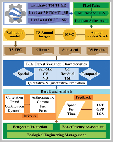
This study developed and applied a main process of evaluating and analyzing TNR forest changes which is shown in Figure 1. Firstly, time-series annual synthetic remote sensing data were generated using Landsat remote sensing data on GEE platform by employing the M-OLS and MVC method. Next, long time-series FFC datasets were constructed based-on machine learning models. Secondly, meteorological, statistical, and remote sensing data products were jointly used to assess and analyze the spatio-temporal variability characteristics, the contribution of drivers of change and feedback effects of TNR forests using Sen-MK, CV, VD, residual trend analysis, and other methods. Finally, the ecological effect assessment of TNR forests and ecological engineering management are discussed.

Figure 1. Flowchart of the analysis of forest cover changes and driving factors in the three-north of China.

3.1. Long time series FFC dataset

This study used GEE to generate long-term FFC datasets according to the following process: (1) To improve the spatial and temporal representativeness of the data and reduce data discrepancy caused by non-sensor factors, image with a sensor imaging time difference or less than 2 days and the containing different surface types were selected for pre-processing. Surface reflectance image pairs from Landsat-7 ETM + and Landsat-8 OLI were uesd, and only good quality pixels were retained. (2) A multi-band joint least squares (M-OLS) approach was used to construct a conversion model (Equation (1)(1) $OL{I}_i=\sum _{i=1}^n{\rho }_i\times ETM{+}_i+{\theta }_i$(1) ) from ETM+ to OLI. This approach achieves consistent conversion of the reflectance between the two sensors while considering the interaction between bands. Although there is no time overlapping imaging between TM and OLI, previous research suggests that the visible light bands of TM and ETM+are equivalent (Flood 2014), so the conversion model built by ETM+and OLI can be used to convert between TM and OLI. (3) To reduce the amount of data processing and improve the processing efficiency, the consistent converted reflectance data were stacked by year to form a year-by-year time series remote sensing image collection; Among them, due to the lower NDVI values of abnormal pixels such as clouds or fog, NDVI is used as an indicator to remove noise elements. The maximum normalized difference vegetation index (NDVI) composite (MVC) was adopted to remove clouds, shadows, or edge pixels in time series Landsat data, and synthesize the annual stacked data into the annual composite data (Myroniuk et al. 2020; Piao et al. 2021). (4) In our previous study (Liu et al. 2021), we developed the FFC estimation model for Landsat 8 imagery based on an ensemble learning algorithm using Gaofen-2 data as a reference, but we did not produce a long-time series FFC data over the entire TNR because of the massive data volume. This study applies this model to produce the TNR long time series FFC dataset using more than 40,000 Landsat images. Composite data and other feature parameters are combined into a data cube consistent with the model input to generate a time series FFC dataset.

(1) $OL{I}_i=\sum _{i=1}^n{\rho }_i\times ETM{+}_i+{\theta }_i$(1)

where:${\rho }_i$ is the conversion coefficient, $ETM{+}_i$ denotes the ith visible band of ETM+ (i = 1,2,3,4,5,6), $OL{I}_i$ denotes the band of the OLI sensor corresponding to the $ETM{+}_i$ band, and θ is a constant term.

3.2. FFC change trend detection and analysis

3.2.1. Sen-Mann-Kendall trend test

The Theil-Sen slope estimator is an nonparametric trend estimate method widely utilized in remote sensing and ecological studies. Unlike paremetric methods, it does not assume any particular data distribution and can provide accurate regression slopes even in the presence of outliers or non-normality. The Mann-Kendall (MK) is a non-parametric test, also known as a distribution-free test. It is insensitive to outliers, and does not require time series data to follow a certain distribution (Pei et al. 2021; Yang et al. 2019; Zhang et al. 2016). Moreover, the Sen-MK trend test allows us to statistically test whether there is a monotonically increasing or decreasing trend within a time-series FFC dataset, providing valuable insight into long-term environmental changes.

3.2.2. Quantification of forest cover change

The coefficient of variation (CV) is a statistical measure that quantifies the ratio of the standard deviation to the mean of a time series data, reflecting the degree of variability or stability of the data over time. In this study, the CV is utilized to characterize the fluctuation level of FFC. Vegetation Dynamics (VD) was used to evaluate the extent of changes in vegetation area between the end and base period of the study. To quantify the degree of change in forests at different time intervals, the FFC is divided into 11 gradients, starting from 0% and with a gradient interval of 10%. The characteristics of forest changes for each FFC gradient are analyzed. Additionally, the land use transition matrix was employed to describe the transition scale of land use types during different periods. It indicates the numbers of different land-use types that remained constant and changed during the study period. In this study, forests with different FFC levels were regarded as different types. According to the 20% interval, FFC was divided into low (L; FFC: 0–20%), medium low (M-L; FFC: 20–40%), medium (M; FFC: 40–60%), medium high (M-H; FFC: 60–80%) and high (H; FFC: 80–100%) (Liu et al. 2018; Zhang and Liang 2014).

3.3. Attribution analysis of FFC changes

3.3.1. Correlation analysis

We assessed the degree of influence of temperature and precipitation on forest cover change by calculating the Pearson correlation coefficient (CC) and partial correlation coefficient (PCC) of FFC with temperature and precipitation. The CC reflects the degree of association between two variables; while the PCC enables the correlation analysis of two variables (FFC and temperature or FFC and precipitation), while controlling for the effect of the other variable (precipitation or temperature), which can provide a better understanding of the relationship among the three (Shi et al. 2021; Zhao et al. 2020).

(2) $r=\frac{{\sum }_{i=1}^n\left(x_i-\bar{x}\right)\left(y_i-\bar{y}\right)}{\sqrt{{\sum }_{i=1}^n\left(x_i-\bar{x}\right)}\sqrt{{\sum }_{i=1}^n\left(y_i-\bar{y}\right)}}$(2)

(3) $r_{Ft,p}=\frac{R_{Ft}-R_{Fp}\ast R_{tp}}{\sqrt{\left(1-R_{Fp}^2\right)\ast \left(1-R_{tp}^2\right)}}$(3)

(4) $r_{Fp,t}=\frac{R_{Fp}-R_{Ft}\ast R_{tp}}{\sqrt{\left(1-R_{Ft}^2\right)\ast \left(1-R_{tp}^2\right)}}$(4)

Where:$\hspace{0.17em}{x}_i$ and $y_i$ represent the values of the two variables $x$ and $y$ involved in the correlation analysis in the ith year; $\bar{x}$ and $\bar{y}$ are the mean values of the variables x and y, respectively; R is the CC of the two elements; $R_{Ft,p}$ represents the PCC between FFC and temperature; $R_{Fp,t}$ represents the PCC between FFC and precipitation; $R_{Ft}$ represents the CC between FFC and temperature; $R_{Fp}$ represents the CC between FFC and P; $R_{tp}$ represents the CC between temperature and precipitation.

3.3.2. The analysis of residual trend

The residual trend method, proposed by Evans and Geerken in 2004, is a widely used approach for analyzing vegetation changes. It is based on the assumption that changes in vegetation cover are closely related to climatic factors (primarily precipitation and temperature) and that the effects of non-climatic factors, such as human activities, can be represented by model residuals – by unexplained changes between vegetation cover indicators and climatic factors (Evans and Geerken 2004; Shi et al. 2021; Wang et al. 2015). In this study, we utilized residual trend method to investigate forest vegetation changes. In the first step, to establish a model that describes the relationship between forest vegetation and climate factors, based on this model, the estimated value of FFC under ideal conditions can be calculated from climate data; however, due to the influence of other factors, there may be differences between the estimated and the actual observed value of FFC. Therefore, in the second step, we calculated the FFC residual, which represents the difference between the estimated and actual values of FFC. In the third step, we conducted a trend analysis on the residuals. The trend of residuals is considered to be unrelated to climate, mainly reflects changes in forest vegetation caused by non-climate factors. By jointly analyzing the trends of observed, estimated and residual values, it is possible to identify the contribution of both climatic and non-climatic factors to forest vegetation change. A positive trend of the residuals indicates that non-climatic factors contribute to the improvement of forest vegetation, while the opposite indicates that non-climatic factors lead to the degradation of forest vegetation (Burrell, Evans, and Liu 2017; Wessels, van den Bergh, and Scholes 2012). However, there are some limitations in the conventional use of this method: Due to the complex response mechanisms between climate factors and vegetation, linear regression cannot accurately model the relationship between climate factors and forest vegetation (Huang and Kong 2016; Shi et al. 2020).

This study is grounded on the assumption that the changes in FFC are impacted by both climatic and non-climatic factors. Firstly, we analyzed the temporal variation trend of temperature, precipitation, and FFC data from 1996 to 2020 and select the pixels with high stability. During this process, we constructed a dataset containing 10,094 samples with temperature and precipitation as predictors and FFC as response variables. Then, considering that random forest (RF) is a machine learning method for multi-decision integration and has obvious advantages in fitting the nonlinear relationships among the covariates (Zhang and Yang 2020), we selected RF to construct an estimation model of FFC and temperature and precipitation. Thus, 70% of the sample data was used as the training set, and 30% of the data is used as the validation set. RMSE served as the evaluation index of the model, which attained a final validation accuracy of RMSE = 0.09. Finally, the value of FFC (C_FFC) under the influence of climate factors is calculated by using the constructed model combined with the temperature and precipitation of TNR. The reference FFC value $\left(\mathrm{O}\mathrm{\_}\mathrm{F}\mathrm{F}\mathrm{C}\right)$ minus the FFC value under the influence of climate change$\mathrm{C}\mathrm{\_}\mathrm{F}\mathrm{F}\mathrm{C}$, the obtained residual ($\mathrm{R}\mathrm{\_}\mathrm{F}\mathrm{F}\mathrm{C}$) can be considered as the influence of non-climate factors including human factors on the FFC ($\mathrm{H}\mathrm{\_}\mathrm{F}\mathrm{F}\mathrm{C}$):

(5) $\mathrm{H}\mathrm{\_}\mathrm{F}\mathrm{F}\mathrm{C}=\mathrm{O}\mathrm{\_}\mathrm{F}\mathrm{F}\mathrm{C}-\mathrm{C}\mathrm{\_}\mathrm{F}\mathrm{F}\mathrm{C}$(5)

To analyze whether the influence of non-climatic factors on the FFC change was positive or negative, this study conducted a pixel-by-pixel trend analysis of the obtained residual sequence, and obtained the spatial distribution pattern of the residual change trend. The trend can reflect the influence of non-climatic factors on the FFC variation. Combined with the FFC change trend $\mathrm{O}\mathrm{\_}\mathrm{F}\mathrm{F}\mathrm{C}$, under the condition that the FFC change trend was significant, the contribution rates of climatic and non-climatic factors to FFC change could be calculated by referring to Equations (6)(6) $\mathrm{C}\mathrm{c}=\frac{\mathrm{S}\mathrm{l}\mathrm{o}\mathrm{p}{\mathrm{e}}_{\mathrm{C}\mathrm{\_}\mathrm{F}\mathrm{F}\mathrm{C}}}{\mathrm{S}\mathrm{l}\mathrm{o}\mathrm{p}{\mathrm{e}}_{\mathrm{O}\mathrm{\_}\mathrm{F}\mathrm{F}\mathrm{C}}}\times 100\mathrm{\%}$(6) and (7(7) $\mathrm{C}\mathrm{h}=\frac{\mathrm{S}\mathrm{l}\mathrm{o}\mathrm{p}{\mathrm{e}}_{\mathrm{H}\mathrm{\_}\mathrm{F}\mathrm{F}\mathrm{C}}}{\mathrm{S}\mathrm{l}\mathrm{o}\mathrm{p}{\mathrm{e}}_{\mathrm{O}\mathrm{\_}\mathrm{F}\mathrm{F}\mathrm{C}}}\times 100\mathrm{\%}$(7) ) (denoted by Cc and Ch, respectively) (Shi et al. 2021; Yang et al. 2017).

(6) $\mathrm{C}\mathrm{c}=\frac{\mathrm{S}\mathrm{l}\mathrm{o}\mathrm{p}{\mathrm{e}}_{\mathrm{C}\mathrm{\_}\mathrm{F}\mathrm{F}\mathrm{C}}}{\mathrm{S}\mathrm{l}\mathrm{o}\mathrm{p}{\mathrm{e}}_{\mathrm{O}\mathrm{\_}\mathrm{F}\mathrm{F}\mathrm{C}}}\times 100\mathrm{\%}$(6)

(7) $\mathrm{C}\mathrm{h}=\frac{\mathrm{S}\mathrm{l}\mathrm{o}\mathrm{p}{\mathrm{e}}_{\mathrm{H}\mathrm{\_}\mathrm{F}\mathrm{F}\mathrm{C}}}{\mathrm{S}\mathrm{l}\mathrm{o}\mathrm{p}{\mathrm{e}}_{\mathrm{O}\mathrm{\_}\mathrm{F}\mathrm{F}\mathrm{C}}}\times 100\mathrm{\%}$(7)

where, $\mathrm{S}\mathrm{l}\mathrm{o}\mathrm{p}\mathrm{e}$ represents the slope of the corresponding time series data with the change of the year, the Sen method is used to calculate the slope, which can improve the robustness and reduce the influence of outliers. Based on the significance of the $\mathrm{O}\mathrm{\_}\mathrm{F}\mathrm{F}\mathrm{C}$ value of FFC and equations (6)(6) $\mathrm{C}\mathrm{c}=\frac{\mathrm{S}\mathrm{l}\mathrm{o}\mathrm{p}{\mathrm{e}}_{\mathrm{C}\mathrm{\_}\mathrm{F}\mathrm{F}\mathrm{C}}}{\mathrm{S}\mathrm{l}\mathrm{o}\mathrm{p}{\mathrm{e}}_{\mathrm{O}\mathrm{\_}\mathrm{F}\mathrm{F}\mathrm{C}}}\times 100\mathrm{\%}$(6) and (7(7) $\mathrm{C}\mathrm{h}=\frac{\mathrm{S}\mathrm{l}\mathrm{o}\mathrm{p}{\mathrm{e}}_{\mathrm{H}\mathrm{\_}\mathrm{F}\mathrm{F}\mathrm{C}}}{\mathrm{S}\mathrm{l}\mathrm{o}\mathrm{p}{\mathrm{e}}_{\mathrm{O}\mathrm{\_}\mathrm{F}\mathrm{F}\mathrm{C}}}\times 100\mathrm{\%}$(7) ), the calculation method for the contribution rate of driving factors is shown in Table 1 (Leroux et al. 2017):

Table 1. Residual trend method to calculate the contribution rate to FFC changes.

$\mathrm{S}\mathrm{l}\mathrm{o}\mathrm{p}{\mathrm{e}}_{\mathrm{O}\mathrm{\_}\mathrm{F}\mathrm{F}\mathrm{C}}$	$\mathrm{S}\mathrm{l}\mathrm{o}\mathrm{p}{\mathrm{e}}_{\mathrm{C}\mathrm{\_}\mathrm{F}\mathrm{F}\mathrm{C}}$	$\mathrm{S}\mathrm{l}\mathrm{o}\mathrm{p}{\mathrm{e}}_{\mathrm{h}\mathrm{\_}\mathrm{F}\mathrm{F}\mathrm{C}}$	Climate Contribution%	Non-climate contribution%
significant increase (p<0.05)	>0	>0	Cc	Ch
	>0	<0	100	0
	<0	>0	0	100
significantly Decrease (p<0.05)	<0	<0	Cc	Ch
	<0	>0	100	0
	>0	<0	0	100

3.4. Evaluating impacts of FFC change

We implemented a spatial-temporal approach (Li et al. 2015; Peng et al. 2014; Yang, Huang, and Tang 2020) to compare the differences between LST, GPP, and land-surface albedo (LSA) of high-FFC forests and adjacent low-FFC forests to quantify the impact of forests on physical processes at the surface. First, to eliminate the effects of different climatic conditions and ensure that the selected pixels had similar climatic backgrounds, we established a square window with an initial edge length of 40 km, centered on a forest pixel with high-FFC. Second, we searched for forest pixels with low-FFC within this window. To mitigate the effect of elevation changes, pixels with an elevation difference >50 m from the central image element were excluded. We calculated the annual average LSA, LST, and GPP values. To account for the possible impact of human activities on the results, the data extracted in this study were mainly pixels with different FFC. The LST, GPP, and LSA differences ($\mathrm{\Delta }LST\mathrm{\Delta }LSA\mathrm{\Delta }GPP$) of forest pixels with different FFC were compared.

(8) $\mathrm{\Delta }LST=LS{T}_{FF{C}_{High}}-LS{T}_{FF{C}_{low}}$(8)

(9) $\mathrm{\Delta }LSA=LS{A}_{FF{C}_{High}}-LS{A}_{FF{C}_{low}}$(9)

(10) $\mathrm{\Delta }GPP=GP{P}_{FF{C}_{High}}-GP{P}_{FF{C}_{low}}$(10)

Taking LST as an example, a positive (negative) $\mathrm{\Delta }LST$ indicates a warming (cooling) effect of increasing forest cover, and the differences in $\mathrm{\Delta }LSA\mathrm{\Delta }GPP$ were similarly defined.

4. Result

4.1. Fractional forest cover spatiotemporal variations

4.1.1. Fractional forest cover mapping and time series trends

The OLI and ETM+ band conversion parameters (Table 2) of the M-OLS regression were obtained. This was applied to ETM+ to obtain the adjusted transformed reflectance data. The performance of the reflectance conversion model was evaluated using independent validation data.

Table 2. ETM+ and OLI multi-band least squares regression (M-OLS) conversion parameters.

Band name	Conversion factor/constant term
OLI_Blue	[0.1495, 0.4948, 0.0579, −0.0271, −0.0112, 0.0184]/0.0001
OLI_Green	[−0.5206, 1.1124, 0.1615, 0.0055, −0.0513, 0.0316]/0.0069
OLI_Red	[−0.5780, 0.4115, 0.9665, −0.0388, −0.0225, 0.0157]/0.008
OLI_Nir	[−0.4978, 0.2105, 0.1033, 0.9571, 0.1265, −0.1269]/0.0101
OLI_SWIR1	[−0.3482, 0.1683, 0.1363, −0.0382, 0.9591, −0.0606]/0.0169
OLI_SWIR2	[−0.3342, 0.1959, 0.1087, −0.045, 0.0127, 0.886]/0.0162

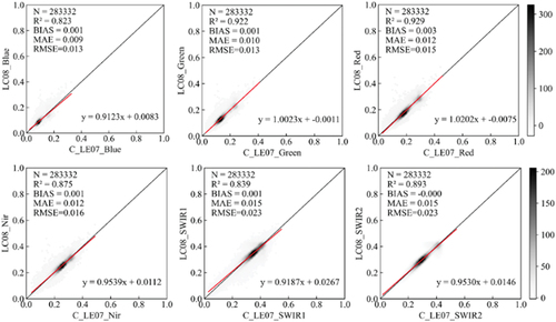
Figure 2 shows the reflectance scatter plot of the ETM+ and OLI raw bands used as the validation data. The horizontal axis of the plot represents the ETM+ band, and the vertical axis represents the OLI band. There was a difference between the bands corresponding to the two sensors, and the blue band had the weakest correlation with a slope of only 0.82. The red band had the strongest correlation. The RMSE values between the two sensor bands were between 0.016 and 0.026. The slopes of the blue band and SWIR1 deviated the most from the 1:1 line, with both < 0.9. Figure 3 shows the conversion result of the M-OLS model. The consistency between several bands showed a high improvement, the slope of the blue band also increased (to > 0.91), and the correlation (R²)between the bands was significantly improved (i.e. all were > 0.8) and their deviations reduced.

Figure 2. Comparison of raw reflectance between ETM+ (LE07) and OLI (LC08).

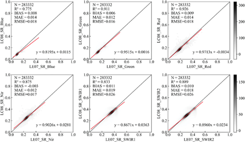
Figure 3. Comparison of ETM+ (C_LE07) and OLI (LC08) reflectance after coefficient adjustment.

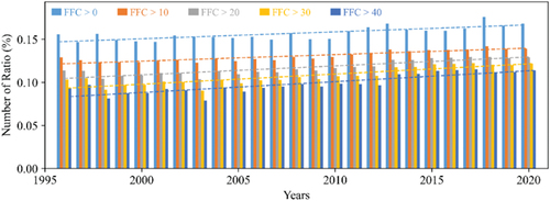
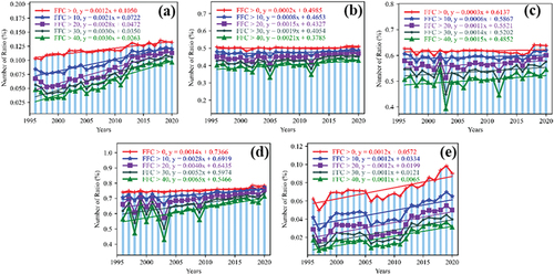
Figure 4 shows the FFC dataset of the TNR from 1996 to 2020. The dataset was generated based on the GEE platform and had the characteristics of spatiotemporal continuity and high spatial resolution (30 m). Meanwhile, considering that in the definition of forest, there are different criteria for canopy cover, in orser to clarify the temporal characteristics of forest cover changes, we set 0, 10%, 20%, 30%, and 40% as gradient thresholds, respectively, obtained forest cover at different thresholds from 1996 to 2020, and performed linear fitting on the time-series forest cover (Figure 5). The results showed that the overall forest area of the TNR fluctuated and increased, with an average annual growth rate of 0.02/10a. Taking the statistical results of the 20% threshold as an example, the forest area in 2003 was the lowest, and the forest cover area in 2018 was the highest over the past 25 years. In Figure 5, 2003 is the first year with the least forest cover since 1996 when the threshold of FFC > 20% is used. Meanwhile, 2010 is the end of the fourth phase of the TNSFP, so the time series are divided into 1996–2003, 2003–2010, and 2010–2020 by using two years, 2003 and 2010, as the time nodes. There was a decreasing trend from 1996 to 2003, and the forest cover increased after 2003. Before 2010, there was an increasing trend in forest cover of 0.022/10a. After 2010, forest cover increased more rapidly, i.e. at 0.03/10a. According to the afforestation area statistics in each province (Tab S12), after 2006, the annual increase in the afforestation area in each province was the factor for the increase in the forest area in TNR after 2010.

Figure 4. The distribution of FFC in the TNR from 1996 to 2020.

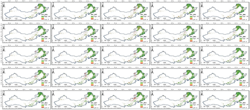
Figure 5. Time series variation characteristics of FFC (10% is the gradient threshold to represent different fraction cover).

4.1.2. Fractional forest cover spatial distributions and changes

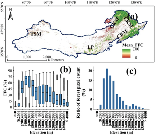
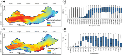
To analyze the relationship between terrain factors and forest spatial distribution, the overall characteristics of the terrain were obtained by calculating the elevation and slope, and the FFC map was overlaid with the elevation map to obtain the spatial characteristics of the forest distribution under different terrain conditions. Figure 6(a) shows that the distribution of the mean FFC of the TNR from 1996 to 2020 had obvious spatial heterogeneity. Figure 6(b) shows the distribution box plot of FFC at different altitudes. In the range of altitudes <200 m, the forest was dominated by low-FFC. At altitudes <800 m, FFC increased with increasing altitude. At altitudes >2000 m, FFC decreased with increasing altitude. According to statistics on the distribution of TNR forests (Figure 6(c)), approximately 2.5% of the forests were distributed at altitudes <200 m and approximately 6.5% were distributed at altitudes >2000 m.

Figure 6. Average spatial distribution of FFC from 1996 to 2020 (a), Boxplot of FFC distribution with elevation, representing the coverage distribution range (b), Characterizing the proportion of forest pixels at different elevations (c).

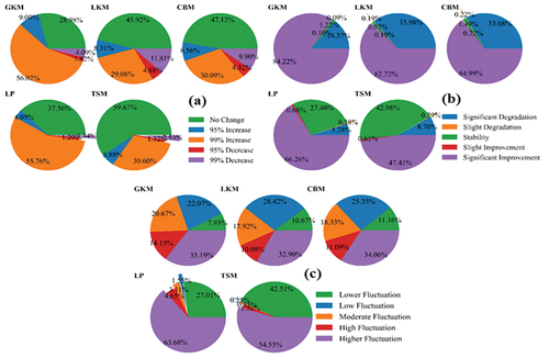
FFC of the TNR showed an overall increasing trend. As shown in Figure 7(a), the regions with significant increases were mainly distributed in the western part of the Tianshan Mountian (TSM), Loess Plateau (LP), and Greater Khingan Mountains (GKM), and there was a significant decreasing trend in the southern region of the Changbai Mountains (CBM) and Lesser Khingan Mountains (LKM). The FFC slope was divided into five categories: very significant increase (slope ≥0.005), significant increase (0.002 ≤ slope < 0.005), no significant change (−0.002 ≤ slope < 0.002), significant decrease (−0.002 ≤ slope < −0.005), or very significant decrease (slope < −0.005) (Figures 7b and 8(a,b)). The area with a very significant increase accounted for 55% (p < 0.05) of the total area. Whereas, approximately 29% showed no significant change. Approximately 15% of the forest cover showed a very significant downward trend (Table S3). Among them, GKM mainly showed a significant increasing trend (84%). However, there was also degradation of approximately 14% in the northern part of GKM, and significantly degraded areas of LKM and CBM accounted for > 30%. The LP and CBM are stable forests that occupy a large proportion. In general, FFC of these areas has mainly been increasing, and forests showing a downward trend exhibited discrete distribution characteristics. From Figure 8(c), it can be seen that approximately 64% of the forest cover in LP exhibited a higher fluctuation, and approximately 55% in TSM; GKM, LKM, and CBM areas were dominated by medium and low fluctuations (i.e. 50%, 57%, and 55%, respectively).

Figure 7. MK change trend of FFC.

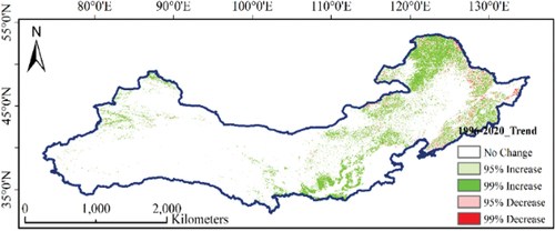
Figure 8. Statistics of FFC change characteristics in TNR sub-region. Trend in sub-regions (a), Slope in sub-regions (b), CV in sub-regions (c).

4.1.3. Dynamic change characteristics of fractional forest cover

Based on FFC, Table 3 and Tab S1 show the degradation and restoration characteristics during different periods. From 1996 to 2000, the forests with FFC of 0, 10–20%, 20–30%, and 70–80% were positive, and the other FFC level of forests were negative, only approximately 2% of low-FFC level forests changed to a higher FFC, and the degraded proportions of M-L and M forests were lower than their restoration proportions. The degradation ratio of M-H and H forests was higher than that of restoration, indicating that forest degradation was more serious during this period. From 2000 to 2005, the VD of the low-FFC group was negative, and that of the high-FFC group was positive. Forest degradation of the M-L FFC, M FFC, and M-H FFC showed slowing trends compared with the previous period, and the proportion of restoration increased significantly. This showed that forest growth had improved and been restored to a certain extent, especially the forests with FFC in the ranges of 80‒90% and 90‒100%. From 2005 to 2010 and 2010 to 2015, the degradation trend slowed, the restoration trend accelerated, and the overall forest coverage increased. The VD from 2005 to 2010 showed a positive change in M and H FFC. From 2010 to 2015, the VD value of 0 showed a negative value, indicating that the area of non-forest land decreased and the area of newly added forestland increased, the decrease in M FFC and the increase in H FFC also indicated improved forest cover during this period. From 2015 to 2020, the overall increasing trend slowed, and the VD of forests with H FFC levels was negative, indicating that the degradation ratio of forests with M FFC levels and above increased during this period. The negative VD value for non-forest land indicated that continuous forestland addition had been taking place. Comprehensive analysis showed that there has been continuous new forest land in this area over the past 25 years. Forests with M FFC levels fluctuated greatly, whereas, forests with H FFC levels showed a trend of initially increasing and then degrading with time. Among them, 2000‒2015 was a period of increasing trends in TNR forest restoration, however, the forest restoration rate decreased after 2015.

Table 3. The dynamic degree of FFC change in the TNR.

	1996–2000	2000–2005	2005–2010	2010–2015	2015–2020
0	0.0024	−0.0009	0.0001	−0.0022	−0.0019
(0,10]	−0.0259	0.0187	−0.0395	0.0155	0.0572
(10,20]	0.0072	−0.0014	−0.0345	−0.0547	0.0147
(20,30]	0.0049	−0.0031	−0.0207	−0.0442	−0.0012
(30,40]	−0.0035	−0.0018	−0.0146	−0.0336	0.0068
(40,50]	−0.0149	−0.0071	0.0041	−0.0237	0.0047
(50,60]	−0.0221	−0.0046	0.0202	−0.0269	−0.0001
(60,70]	−0.0031	−0.0109	0.0359	−0.0316	0.0094
(70,80]	0.011	−0.0008	0.0294	0.0039	0.012
(80,90]	−0.0406	0.0371	0.0062	0.119	−0.0016
(90,100]	−0.0875	0.0463	0.0054	0.6083	−0.0283

The gradient trend of the time series can represent the temporal characteristics of forest changes, and when combined with statistical data, the reasons for forest changes can be explored and analyzed. FFC of LP showed an overall upward trend (Figure 9a), and the forests with L FFC (0‒30%) showed a trend of initially increasing and then decreasing, forests with the FFC of 30‒50% fluctuated greatly, increasing from 2000 to 2010 and decreasing after 2010. Forests with M and H FFC (50‒100%) showed overall upward trends, with a higher rate of increase after 2010 than before 2010, indicating that the forest vegetation in this area greatly improved after 2010. The inter-annual slope of FFC in the CBM region over the past 25 years was from 0.02% to 0.2%, and the overall upward trend was not obvious (Figure 9b). Forests with an FFC levels of 40‒50% showed a significant decline after 2010, and according to the forest fire statistics in this area (Tab S13 Tab S14), the area of forests affected by fires after 2010 was significantly higher than that before 2010. Combined with the forest changes, it can be considered that fires in this area have had a greater impact on forests with M and L FFC. According to Figure 9(c), forest cover in the LKM exhibited a relatively gentle upward trend. Combined with the statistics (Tab S13 Tab S14) of forest change data in the region, fire was the main factor for fluctuations in the region in 2003. Forests with M and L FFC showed greater instability, forest change with an FFC levels of 60‒80% had obvious time nodes, whereby it showed an upward trend before 2010 and subequently decreased. Forests with H FFC (80‒100%) showed an upward trend. The above analyses showed that forests with H FFC in this area had good stability, whereas, forests with M and L FFC were easily disturbed and fluctuated greatly. The GKM analysis showed an overall upward trend. Figure 9(d) shows that large fluctuations occurred from 1998 to 2003. Combined with the forest change statistics (Tab S13 Tab S14), the higher number of fires and burned areas in the region in 2003 were the main disturbance factors. Since 2015, Inner Mongolia, Jilin, and other regions have gradually stopped commercial logging of natural forests, and the increasing trend of forests with different FFC level grades in the region after 2015 shows that this measure has had a positive effect on improving forest coverage. Overall, the TSM forests showed a fluctuating and increasing trend (Figure 9e); however, there was a significant decrease in 2005. Combining the data (Tab S12, Tab S13, Tab S14, Tab S15), it can be seen that the number of fires in this area increased since 2004, and that 2008‒2016 was a period of high incidence of insect pests in this area. The area maintained a relatively high afforestation level after 2010, the number of fires gradually decreased after 2012, and the area affected by biological disasters gradually decreased after 2016. All of these factors have been beneficial to forest restoration in this area and have contributed to the increase in the forest area.

Figure 9. Temporal variation characteristics of FFC at different levels in sub-regions.

4.2. Relative contributions of climate and anthropogenic activities

4.2.1. Correlation analysis of fractional forest cover with temperature and precipitation

The spatial distribution of the annual average precipitation and air temperature of the TNR over the past 25 years is shown in Figure 10(a,c). We overlayed FFC with annual precipitation and air temperature maps to analyze the relationship between FFC, precipitation, and air temperature. Figure 10(b) shows a boxplot of the relationship between precipitation and FFC distribution. The forests with L FFC levels were dominant in areas with precipitation <370 mm. Forests with precipitation between 370 and 410 mm showed an increasing trend toward high FFC, and were dominated by M and H FFC in areas with precipitation >410 mm. According to statistics, 30% of the forest pixels were distributed below the 370 mm precipitation line and 70% of the forest pixels were above the 370 mm precipitation line. Figure 10(f) shows a boxplot of the relationship between air temperature and the FFC distribution. It can be concluded that the forest was sparsely distributed in the area where the air temperature was < −5°C. When the temperature was in the range of −5 to 0°C, combined with Figure 6, the forest was mainly dominated by M and H FFC. With the increase in temperature, the distribution of forests tended to be stable, whereas, the FFC levels of forests decreased in areas with temperatures > 10°C. Based on the spatial distribution patterns of temperature and precipitation and their distribution law with FFC, it can be concluded that the growth and distribution of forest vegetation were inseparable from water and heat conditions.

Figure 10. Spatial pattern of annual precipitation and temperature in TNR. (a) Mean annual precipitation, (b) The relationship between FFC and precipitation distribution, (c) Mean annual temperature, (d) The relationship between FFC and air temperature distribution.

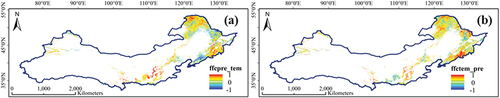
Partial correlation (Pc) analysis was used to explore the independent correlations between precipitation, temperature, and FFC (Figure 11). Among them, the Pc was positive between FFC and precipitation in the forest cover area of the LP, the northern and eastern areas of the GKM, the central and northern areas of the CBM, and the TSM, indicating that precipitation had a promoting effect on FFC in these areas when temperature was not considered. FFCs in the central and southern LKM, southern CBM, and southeastern GKM regions showed negative partial correlations with precipitation, indicating that precipitation negatively affected forest growth in these regions. Figure 11(b) shows the distribution of the Pc coefficient between FFC and temperature without considering the precipitation factor. 70.7% of the forest cover areas showed a positive correlation. These areas were mainly distributed in the east of LP, north of GKM, west and south, east of LKM, south of CBM Region, and in the TSM region. Approximately 28.5% of the forest cover showed a negative correlation (Tab S9 and Tab S10), distributed in the western part of the LP, in the middle of the GKM, and in the border area between the LKM and the CBM. The Pc between precipitation and FFC was higher than that between temperature and FFC. However, forests had different responses to precipitation and temperature due to different hydrothermal conditions in different regions. In LP, there was aridity and minimal rainfall and the hydrothermal conditions were sufficient. Precipitation could promote forest vegetation growth in this area, and the temperature increase had an inhibitory effect on FFC. In the southern part of CBM, it was humid and rainy, and the change in hydrothermal conditions affected vegetation growth by affecting plant photosynthesis, thus affecting the FFC change. However, in the TSM, the hydrothermal and water vapor conditions were lower than in other regions. Therefore, precipitation and temperature could simultaneously promote forest vegetation growth in the TSM region.

Figure 11. Partial correlation between FFC and precipitation (a) and temperature (b).

4.2.2. Impact of climate and anthropogenic activities on fractional forest cover

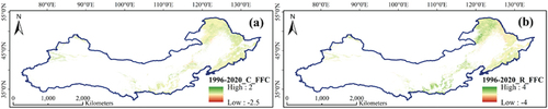
Figure 12(a) shows the potential FFC (C_FFC) variation trend under the influence of climate simulated by the model established between climate factors and FFC. Figure 12(b) shows the residual (R_FFC) between O_FFC and C_FFC, which can be considered as the impact of non-climatic factors on FFC, including human activities (logging, planting, etc.), biological disasters (diseases, pests, species invasion, etc.), and forest fires. Calculation of the change trends of C_FFC and R_FFC showed a significant difference between C_FFC and O_FFC: > 56% of the areas showed a very significant decline, including the northern and southern parts of GKM, most of the CBM, and the southern part of LP,only 41% of the areas showed a significant increase (LKM and TSM), R_FFC showed an upward trend overall, indicating that non-climatic factors played a positive role in the increase of TNR forests, and most areas of LP and GKM showed the most obvious trend, and most areas of the LKM showed a downward trend. Owing to the high population density and intensive human activities in the areas where the mountains and plains meet in the southern part of the GKM and the northern part of CBM, the forests in these areas are more vulnerable to human activities, especially urban expansion, and the increase in agricultural area has had negative effects on forest change.

Figure 12. Variation trend of FFC under the influence of climate (a) and non-climate (b) from 1996 to 2020.

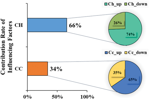
Figure 13 shows the spatial distribution of the contribution rates of the influencing factors obtained using the contribution rate estimation model. The main area where climatic factors were influential was in the northeast (Figure 13(a,c,e)), including the southern part of the GKM, LKM, and part of the CBM, which mainly reflected a positive effect, whereas, the northern part of the GKM and the southern part of the CBM showed a negative effect with discrete distribution characteristics. The non-climatic factors mainly affected a wider area (Figure 13(b,d,f)), primarily in the central part of the GKM, LKM, and Yanshan to the LP and other areas. According to statistics (Figure 14), the relative contribution rate of climatic factors to FFC changes was 34%, of which the proportion of positive effects was 65% and that of negative effects was 35%. Overall, climate factors positively affected changes in FFC, and the relative contribution rate of non-climatic factors was 66%, of which the positive and negative effects were 74% and 26%, respectively, which also had a positive effect on the change in FFC. Based on the contribution rate analysis, it can be concluded that both climatic and non-climatic factors have had a positive effect on FFC, and that non-climatic factors have played a leading role in the change in FFC in the past 25 years.

Figure 13. Distribution of contribution rate. climate factor (a), Non-climate factor (b), Positive effect of climate factor (c), Negative effect of climate factor (d), Positive effect of non-climate factor (e), Negative effect of non-climate factor (f).

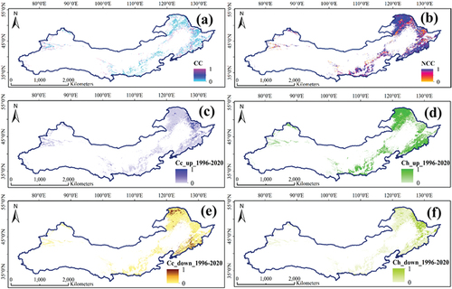
Figure 14. Statistics of the contribution rate of influencing factors in the change of FFC.

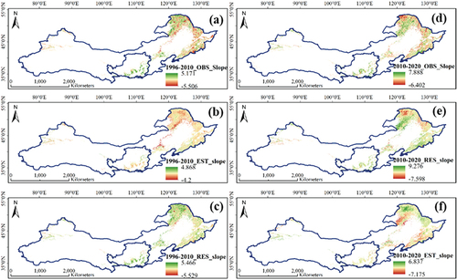
The periods from 2001 to 2010 and 2011 to 2020 were the fourth and fifth phases of the TNSFP project, respectively. Taking 2010 as the time node, the changes in FFC in the two periods of 1996‒2010 and 2010‒2020 were analyzed. As shown in Figure 15, the growth trends of the northern GKM and LP were significantly higher than that of other regions from 1996 to 2010, and that after 2010, the growth trend of FFC of the TNR began to decline. Except for the southern part of the GKM, the growth areas showed a discrete distribution. As shown in Figure 15(b,e), the influence of non-climatic factors on FFC of the two periods was mainly positive feedback, especially before 2010, most of the forests showed an increasing trend, however the northern part of the GKM showed a downward trend after 2010. Combined with Figure 15(c), it can be concluded that the downward trend was mainly caused by non-climatic factors. Overall FFC of the TNR showed an increasing trend in both periods, and the overall growth trend after 2010 was higher than that before 2010. However, it was also found that the growth trend of LP before 2010 was higher than that after 2010.

Figure 15. The changing trend of FFC in the TNR. (a) 1996–2010 O_FFC, (b) 1996–2010 C_FFC, (c) 1996–2010 R_FFC, (d) 2010–2020 O_FFC, (e) 2010–2020 C_FFC, (f) 2010–2020 R_FFC.

4.3. Consequences of FFC changes

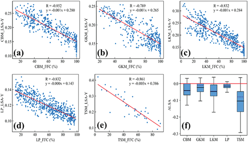
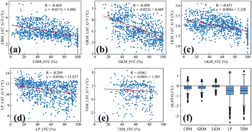
We evaluated the environmental consequences of FFC changes. An increase in FFC can significantly reduce the surface albedo, which is a warming effect. Figure 16 shows a strong negative correlation between FFC and LSA in each region of the TNR, i.e. the higher the FFC, the lower the LSA. This was because, under normal circumstances, the brightness of surfaces such as grassland and bare soil is higher than that of forest, and the forest with low FFC level was affected by grass or bare soil in the background and had a higher albedo, theus, albedo decreased when FFC increased. Figure 16(f) shows the quartile map of the effect of FFC on LSA (ΔLSA) in different regions of the TNR. The black horizontal line in Figure 16(f) represents the mean value, the red dotted line represents the zero value line, and a value < 0 indicates that ΔLSA was negative. It can be concluded that the increase in FFC had a reducing effect on the albedo of the region overall, among which FFC of the TSM had the most obvious reduction effect on LSA (−0.104[0.077]), and the forest in the LP area had the lowest reduction effect on LSA (−0.015[0.013]).

Figure 16. Relationship between FFC and LSA.

Increases in FFC have a net cooling effect, largely due to the increased evapotranspiration despite the albedo warming effect. Figure 17 shows the relationship between FFC and annual average LST, which showed different degrees of negative correlation in different regions of the TNR, indicating a cooling effect with an increase in FFC. The effects of forests in the GKM, LKM, and CBM regions on LST were lower than those in the LP and TSM regions, i.e. the increase in FFC in the LP and TSM regions had a more obvious cooling effect. Figure 17(f) shows a quartile map of the effect of forests in different regions on LST (ΔLST). The forests in the LP area had the most obvious cooling effect. Although there are some warming samples in other areas, the average value was negative, therefore, the overall impact was a cooling effect. We further analyzed the seasonal temperature changes in these areas (Tab S11), and FFC had the most obvious cooling effect in summer, during which the ΔLST of the first three quarters of GKM, LKM, and CBM were all negative; however, these were positive in winter, indicating that the increase in FFC manifested as a warming effect in winter. The LP and TSM regions exhibited cooling effects.

Figure 17. Relationship between FFC and LST.

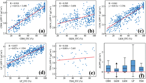
FFC is a useful indicator of vegetation productivity. Figure 18 shows the correlation between forest coverage and GPP, and that the increase in FFC had a positive effect on the increase in GPP. There were obvious positive correlations between FFC and GPP in CBM, GKM, LKM, and LP, and FFC in the TSM region was positively (but not obviously) correlated with GPP. Figure 18(f) shows a quartile map of the forest effect on GPP (ΔGPP). Overall, the increase in FFC had a positive effect on GPP; however, there were significant differences in different regions. The change in FFC in the LP region caused the largest change in GPP, whereas, in the GKM region, the increase in GPP caused by FFC was the smallest (ΔGPP = 0.168 gC/m³).

Figure 18. Relationship between FFC and GPP.

5. Discussion

This study utilized FFC data to investigate the forest changes in the TNR, which demonstrated the strengths of the FFC dataset in representing forest change information and providing clear insight into the characteristics, status, and trends of forest distribution in the TNR.

5.1. Discussion of impact factors

5.1.1. Climatic factors

In the TNR, temperature and precipitation have had significant impacts on FFC change over the past 25 years, with their effects exhibiting spatial heterogeneity (Peng et al. 2021). Specifically, in the midwest of the TNR, precipitation has had a stronger positive effect than temperature’s negative impact on FFC change. which can be attributed to the climatic conditions and geographical location of the TNR. The eastern part of the TNR is characterized by humid and rainy conditions, where forest growth has a higher demand for light. In contrast, the central and western parts of the TNR generally experience less precipitation but sufficient sunlight, leading to excess light and heat that result in soil evaporation exceeding precipitation levels. High temperatures accelerate plant transpiration and increase the respiration rate of vegetation, thereby accelerating dry matter consumption. Plants are subjected to water stress and experience physiological drought, which affects plant growth, resulting in reduced FFC level. Precipitation plays a crucial role in alleviating water stress and increasing soil moisture, making vegetation in these areas more sensitive to the precipitation level (Jiang et al. 2020; Zhang et al. 2021). In the eastern region, annual average precipitation is abundant; however, light and heat are lacking, resulting in higher sensitivity of forest vegetation to temperature in this region.

5.1.2. Anthropogenic drivers

In addition to climatic factors, anthropogenic activities are considered to be an important factor in VD (Wei et al. 2022). In the TNR, on one hand, through afforestation activities, the forest coverage rate increased from 5.05% in 1977 to 13.57% in 2020, and has continued to increase (Tab S12). Several ecological projects in northern China are of great significance for increasing the total amount of forest resources, controlling land desertification, reducing soil erosion, and increasing forest carbon sequestration. On the other hand, the implementation of ecological protection policies and the need for production development have affected the restrictive effect of natural geographical conditions on the change in the FFC pattern, i.e. flat, low altitude (<200 m), and adequate water and heat conditions suitable for forest growth areas. As a result of increased human activities, forest vegetation in these areas was sparse or even non-existent, and the rate of forest growth was higher in mountainous areas with steeper slopes than in areas with flat terrain. For example, in the LP area, the slopes of the main reforestation areas are > 15°, and the relative proportion of forest cover increased with the increase in slope. This is because as the human population has increased, urbanization and agricultural cultivation activities have expanded, and flat terrain areas have been used more as areas for human production-related activities. In areas with large slopes, the terrain fluctuates violently, soil erosion becomes more intense, and soil barrenness gradually deepens, making it increasingly unsuitable for agricultural production and cultivation, therefore, people occupy flat land for development. At the same time, high-slope areas are also fully utilized to carry out suitable afforestation and grass-planting projects, which can improve the vegetation coverage in these areas and further improve soil and water conditions, resulting in sparse forest coverage in low-altitude and flat areas, and a gradual increase in forest cover in high-altitude and large sloped areas.

5.1.3. Natural factors other than climatic factors

Forest degradation is driven by several factors, including aging trees whose protective capacity declines, particularly in the early stage of the shelterbelt project that is over 30 years old. In the TNR, drought, water shortage, and poor soil and water conditions prevail, causing instability and degradation of stand structure. These unfavorable conditions also pose challenges for afforestation efforts. The frequency and extent of forest fires, prevention and control of forest diseases, insects, and rodents, and the forest resources of the TNR were counted (Tab S12, Tab S13, Tab S14, Tab S15). TNR is an area with a high incidence of forest fires. Comparing the relationship between the temporal changes of FFC and forest fire, it was found that they had obvious temporal similarity, indicating that fire has been a major natural factor causing forest degradation or loss. Among them, the areas of forest fire damage in Heilongjiang and Inner Mongolia accounted for > 97%, and the four periods of 2003‒2004, 2007‒2008, 2011, and 2018 were periods of high incidence of forest fires in this region. Pests have also had a significant impact on FFC of the TNR, i.e. more than the impact of fire. The areas where pest disasters occurred were mainly concentrated in Inner Mongolia and Xinjiang regions, and have been due to the relatively single species of trees. For example, in Xinjiang region, spruce woodland accounted for 45% of the entire forest area. Dominance of a single tree species could easily cause the spread of pests and diseases, and the forest loss caused by factors such as forest fires could further increase the risk of pests and diseases. In the eastern part of the TNR, the area of disasters was also higher than in other areas because of the larger forest area. The area of biological disasters in Inner Mongolia’s forests peaked in 2014‒2015, and the Yanshan area had a relatively high area of biological forest disasters from 2011‒2017. In general, disturbance of the TNR due to biohazards has been one of the main natural factors for the reduction in FFC.

5.2. Feedback effects on forests

Changes in forest cover affect the climate by altering biogeochemical (e.g. atmospheric CO2 concentration) and biogeophysical (surface albedo, surface temperature, roughness length, and evapotranspiration) processes (Godinho et al. 2016; Peng et al. 2014; Zhang et al. 2021). LST has a strong coupling relationship with the energy radiation and thermodynamic properties of the Earth’s surface, and a higher sensitivity than air temperature to changes in vegetation density (Li et al. 2021; Yang, Huang, and Tang 2020), which were used to characterize the changes in climate caused by changes in forest cover (Peng et al. 2014). LSA determines the amount of solar radiation absorbed by the surface. The consumption of these energy as latent heat and sensible heat fluxes is controlled by vegetation activities and soil water conditions. Therefore, LSA is the main biogeophysical driving force that causes climate change. The change of forest vegetation cover plays a key role in climate change by affecting the energy and water balance (Alibakhshi et al. 2020; Godinho et al. 2016; He et al. 2018). GPP determines the initial material and energy of terrestrial ecosystems, and changes in forest cover directly or indirectly affect ecosystem productivity.

Analysis of the feedback effects of FFC changes in this study showed the same characteristics caused by changes in FFC in different regions of the TNR, such as the same trends in annual LSA, LST, and GPP. Due to differences in climatic conditions, latitude, and other factors, FFC changes have had different degrees of impact on LSA, LST, and GPP in different regions. FFC of GKM, LKM, and CBM was mainly characterized by warming in winter. This was because the radiative and non-radiative effects of afforestation on surface temperature differ at different latitudes. In winter, the proportion of non-radiative effects at high latitudes is small and the radiation effect is dominant, therefore, the effect of afforestation on the surface temperature is a warming effect. Enhanced evapotranspiration during the growing season results in stronger non-radiative effects and, therefore, stronger cooling effects. Forest vegetation productivity is also related to the forest type (Feng et al. 2022); therefore, the changes in GPP caused by changes in FFC showed differences in various regions of the TNR.

5.3. Limitations and shortcomings

Complex interactions exist between human activity and climate change. This study conducted an independent analysis of their impacts on forest change, ignoring their mutual influence, which may have impacted the accuracy of the estimation of the contribution rate of forest change. The response of vegetation, climate, and ecosystems is a complex and interactive process. In this study, only temperature and precipitation were considered, thereby simplifying the limiting factors that affect forest vegetation growth. By considering the effects of topography (slope and slope direction), economy, population, policy, and other climatic factors (CO₂, solar radiation, sunshine hours, etc.) on forest vegetation, a deeper and more precise explanation of the causes of forest change can be obtained. The resolution of the FFC data used in this study was 30 m, whereas the resolution of other data was 500 m or 1 km. To maintain consistency between the data, FFC was resampled to 1 km, which would have caused a lack of data, and at the same time would have reduced the ability to extract the change information on a fine spatial scale. Thus, there is uncertainty in the estimation results. As the resolution of various data types increases, data with consistent resolution will reduce the uncertainty and improve the accuracy of. In addition, this study used the inter-annual synthesis of Landsat to construct annual FFC. Forest vegetation in the TNR is of multiple types which have different growth characteristics in different seasons, and the monsoon-type climate of the TNR also causes obvious hydrothermal differences in different seasons. Thus, they will have different interactions and responses in different seasons. Conducting research on seasonal forest cover changes is conducive to revealing the response patterns of forest and climate change as well as mutual driving, revealing the cycle and operation mechanism of the ecosystem in the region, and further guiding the construction of scientific ecological engineering implementation plans.

6. Conclusions

Based on long time series, 30-m resolution fractional forest cover data combined with multi-source data and integrated with multiple analysis methods, this study revealed the spatiotemporal variation in forests of the three-north regions based on pixel and regional scales.

The trend analysis by time period demonstrated the growth status and change characteristics of the forests in three-north regions. Fractional forest cover showed a decreasing trend before 2003 and an increasing trend from 2003 to 2017. The increasing trend after 2010 was stronger than that before 2010. The stability analysis showed that 56% of the forests were in a state of low-to-medium volatility, mainly in the northeast. The Loess Plateau and Tianshan Mountian areas mainly showed high or higher fluctuations, among which the forest vegetation of Loess Plateau was more unstable owing to the influence of climatic factors, whereas, the forest cover fluctuation in the Tianshan Mountian area was caused by pests and diseases. Vegetation dynamics were combined with a transition matrix to jointly analyze the forest changes of each fractional cover level. After 2017, the transition of high-density forests to medium-density forests indicated that high-density forests were degrading. Medium-density forests did not shift to low-density forests, indicating that high-density forests were in the early stages of degradation. It may be that forest aging led to a decline in the forest, resulting in a decrease in fractional cover.

The climate data trend showed that the temperature in the three-north regions has been increasing. The correlation analysis showed that the correlation between precipitation and fractional forest cover in this region was higher than that between temperature and fractional forest cover. Based on the residual estimation concept, a method for estimating the contributions of climatic and non-climatic factors was developed using machine-learning methods. The driving factors affecting fractional forest cover were analyzed, and the results showed that non-climatic factors (including human factors) played a dominant role in the impact of fractional forest cover (contribution rate = 66%), and that the contribution rate of climatic factors was 34%. Among non-climatic factors, forest fires were one of the main factors affecting forest fluctuations in the Greater Khingan Mountains and Lesser Khingan Mountains regions. The use of a single tree species for artificial afforestation is likely to cause harmful biological disasters in the forests of Xinjiang and Inner Mongolia, thus causing fractional forest cover fluctuations in these areas. The impact of human factors on the distribution and change of forest cover is complex, among which afforestation activities have been the most direct factor in the increase in forest cover in the three-north regions. However, human intervention has restricted the effects of natural geographical conditions on changes in the fractional forest cover pattern, the most obvious of which is that the increase rate of forests in mountains with higher slopes is higher than that of areas with flat terrain. This is because people occupying flat land for production and living activities also make full use of high-slope areas for suitable afforestation and grass-planting projects, hence, the forest coverage in high-altitude and high-slope areas gradually increases. By analyzing the feedback effect of fractional forest cover, it can be concluded that the increase in fractional forest cover has had a positive effect on the overall ecology of the three-north regions, that is, the improvement of forest vegetation coverage through ecological projects such as afforestation has increased vegetation productivity, and can also have a cooling effect on the surface.

Data and codes availability statement

Data available on request from the authors

Acknowledgments

We thank the Global LAnd Surface Satellite (GLASS) team for providing the products to the public (http://glass.umd.edu/index.html, http://glass-product.bnu.edu.cn/index.html). Thanks for the data support provided by the National Qinghai-Tibet Plateau Scientific Data Center (http://data.tpdc.ac.cn). Thanks to the National Bureau of Statistics and China Forestry Information Network for the statistical yearbook data (http://www.stats.gov.cn/tjsj/ndsj/, http://www.lknet.ac.cn/).

Disclosure statement

No potential conflict of interest was reported by the authors.

Supplementary material

Supplemental data for this article can be accessed online at https://doi.org/10.1080/15481603.2023.2300214.

Additional information

Funding

This work was supported by the The Open Research Program of the International Research Center of Big Data for Sustainable Development Goals [No. CBAS2022ORP01]; The National Natural Science Foundation of China [No. 42090011].

References

- Alibakhshi, S., B. Naimi, A. Hovi, T. W. Crowther, and M. Rautiainen. 2020. “Quantitative Analysis of the Links Between Forest Structure and Land Surface Albedo on a Global Scale.” Remote Sensing of Environment 246:111854. https://doi.org/10.1016/j.rse.2020.111854.
- Amarnath, G., S. Babar, and M. S. R. Murthy. 2017. “Evaluating MODIS-vegetation continuous field products to assess tree cover change and forest fragmentation in India – A multi-scale satellite remote sensing approach.” The Egyptian Journal of Remote Sensing & Space Science 20 (2): 157–26. https://doi.org/10.1016/j.ejrs.2017.05.004.
- Bastin, J.-F., Y. Finegold, C. Garcia, D. Mollicone, M. Rezende, D. Routh, C. M. Zohner, and T. W. Crowther. 2019. “The Global Tree Restoration Potential.” Science 365 (6448): 76–79. https://doi.org/10.1126/science.aax0848.
- Bearup, L. A., R. M. Maxwell, D. W. Clow, and J. E. McCray. 2014. “Hydrological Effects of Forest Transpiration Loss in Bark Beetle-Impacted Watersheds.” Nature Climate Change 4 (6): 481–486. https://doi.org/10.1038/nclimate2198.
- Bonan, G. B. 2008. “Forests and Climate Change: Forcings, Feedbacks, and the Climate Benefits of Forests.” Science 320 (5882): 1444–1449. https://doi.org/10.1126/science.1155121.
- Burrell, A. L., J. P. Evans, and Y. Liu. 2017. “Detecting Dryland Degradation Using Time Series Segmentation and Residual Trend Analysis (TSS-RESTREND).” Remote Sensing of Environment 197:43–57. https://doi.org/10.1016/j.rse.2017.05.018.
- Coggins, S. B., N. C. Coops, T. Hilker, and M. A. Wulder. 2013. “Augmenting Forest Inventory Attributes with Geometric Optical Modelling in Support of Regional Susceptibility Assessments to Bark Beetle Infestations.” International Journal of Applied Earth Observation and Geoinformation 21:444–452. https://doi.org/10.1016/j.jag.2012.06.007.
- Collalti, A., A. Ibrom, A. Stockmarr, A. Cescatti, R. Alkama, M. Fernandez-Martinez, G. Matteucci, et al. 2020. “Forest Production Efficiency Increases with Growth Temperature.” Nature Communications 11 (1): 5322. https://doi.org/10.1038/s41467-020-19187-w.
- Connette, G., P. Oswald, M. Songer, and P. Leimgruber. 2016. “Mapping Distinct Forest Types Improves Overall Forest Identification Based on Multi-Spectral Landsat Imagery for Myanmar’s Tanintharyi Region.” Remote Sensing 8 (11): 882. https://doi.org/10.3390/rs8110882.
- Cook-Patton, S. C., S. M. Leavitt, D. Gibbs, N. L. Harris, K. Lister, K. J. Anderson-Teixeira, R. D. Briggs, et al. 2020. “Mapping Carbon Accumulation Potential from Global Natural Forest Regrowth.” Nature 585 (7826): 545–550. https://doi.org/10.1038/s41586-020-2686-x.
- Crouzeilles, R., M. Curran, M. S. Ferreira, D. B. Lindenmayer, C. E. Grelle, and J. M. Rey Benayas. 2016. “A Global Meta-Analysis on the Ecological Drivers of Forest Restoration Success.” Nature Communications 7 (1): 11666. https://doi.org/10.1038/ncomms11666.
- Curtis, P. G., C. M. Slay, N. L. Harris, A. Tyukavina, and M. C. Hansen. 2018. “Classifying Drivers of Global Forest Loss.” Science 361 (6407): 1108–1111. https://doi.org/10.1126/science.aau3445.
- Czerwinski, C. J., D. J. King, and S. W. Mitchell. 2014. “Mapping Forest Growth and Decline in a Temperate Mixed Forest Using Temporal Trend Analysis of Landsat Imagery, 1987–2010.” Remote Sensing of Environment 141:188–200. https://doi.org/10.1016/j.rse.2013.11.006.
- Danneyrolles, V., S. Dupuis, G. Fortin, M. Leroyer, A. de Romer, R. Terrail, M. Vellend, et al. 2019. “Stronger Influence of Anthropogenic Disturbance Than Climate Change on Century-Scale Compositional Changes in Northern Forests.” Nature Communications 10 (1): 1265. https://doi.org/10.1038/s41467-019-09265-z.
- De Keersmaecker, W., S. Lhermitte, L. Tits, O. Honnay, B. Somers, and P. Coppin. 2015. “A model quantifying global vegetation resistance and resilience to short-term climate anomalies and their relationship with vegetation cover.” Global Ecology and Biogeography 24 (5): 539–548. https://doi.org/10.1111/geb.12279.
- Domke, G. M., S. N. Oswalt, B. F. Walters, and R. S. Morin. 2020. “Tree Planting Has the Potential to Increase Carbon Sequestration Capacity of Forests in the United States.” Proceedings of the National Academy of Sciences of the United States of America 117 (40): 24649–24651. https://doi.org/10.1073/pnas.2010840117.
- D’Orangeville, L., D. Houle, L. Duchesne, R. P. Phillips, Y. Bergeron, and D. Kneeshaw. 2018. “Beneficial Effects of Climate Warming on Boreal Tree Growth May Be Transitory.” Nature Communications 9 (1): 3213. https://doi.org/10.1038/s41467-018-05705-4.
- Doughty, C. E., D. B. Metcalfe, C. A. J. Girardin, F. F. Amézquita, D. G. Cabrera, W. H. Huasco, J. E. Silva-Espejo, et al. 2015. “Drought impact on forest carbon dynamics and fluxes in Amazonia.” Nature 519 (7541): 78–82. https://doi.org/10.1038/nature14213.
- Ehbrecht, M., D. Seidel, P. Annighofer, H. Kreft, M. Kohler, D. C. Zemp, K. Puettmann, et al. 2021. “Global Patterns and Climatic Controls of Forest Structural Complexity.” Nature Communications 12 (1): 519. https://doi.org/10.1038/s41467-020-20767-z.
- Evans, J., and R. Geerken. 2004. “Discrimination Between Climate and Human-Induced Dryland Degradation.” Journal of Arid Environments 57 (4): 535–554. https://doi.org/10.1016/S0140-1963(03)00121-6.
- Fathian, F., Z. Dehghan, M. H. Bazrkar, and S. Eslamian. 2016. “Trends in Hydrological and Climatic Variables Affected by Four Variations of the Mann-Kendall Approach in Urmia Lake Basin, Iran.” Hydrological Sciences Journal 1–13. https://doi.org/10.1080/02626667.2014.932911.
- Feng, Y., Q. Liu, Y. Qu, and S. Liang. 2016. “Estimation of the Ocean Water Albedo from Remote Sensing and Meteorological Reanalysis Data.” IEEE Transactions on Geoscience & Remote Sensing 54:850–868. https://doi.org/10.1109/TGRS.2015.2468054.
- Feng, Y., B. Schmid, M. Loreau, D. I. Forrester, S. Fei, J. Zhu, Z. Tang, et al. 2022. “Multispecies Forest Plantations Outyield Monocultures Across a Broad Range of Conditions.” Science 376 (6595): 865–868. https://doi.org/10.1126/science.abm6363.
- Flood, N. 2014. “Continuity of Reflectance Data Between Landsat-7 ETM+ and Landsat-8 OLI, for Both Top-Of-Atmosphere and Surface Reflectance: A Study in the Australian Landscape.” Remote Sensing 6 (9): 7952–7970. https://doi.org/10.3390/rs6097952.
- Forzieri, G., V. Dakos, N. G. McDowell, A. Ramdane, and A. Cescatti. 2022. “Emerging Signals of Declining Forest Resilience Under Climate Change.” Nature 608 (7923): 534–539. https://doi.org/10.1038/s41586-022-04959-9.
- Gadedjisso-Tossou, A., K. Adjegan II, and A. K. M. Kablan. 2021. “Rainfall and Temperature Trend Analysis by Mann–Kendall Test and Significance for Rainfed Cereal Yields in Northern Togo.” Science 3 (1): 17. https://doi.org/10.3390/sci3010017.
- Gao, W. Q., X. D. Lei, M. W. Liang, M. Larjavaara, Y. T. Li, D. L. Gao, and H. R. Zhang. 2021. “Biodiversity Increased Both Productivity and Its Spatial Stability in Temperate Forests in Northeastern China.” The Science of the Total Environment 780:146674. https://doi.org/10.1016/j.scitotenv.2021.146674.
- Gao, W., C. Zheng, X. Liu, Y. Lu, Y. Chen, Y. Wei, and Y. Ma. 2022. “NDVI-Based Vegetation Dynamics and Their Responses to Climate Change and Human Activities from 1982 to 2020: A Case Study in the Mu Us Sandy Land, China.” Ecological Indicators 137:108745. https://doi.org/10.1016/j.ecolind.2022.108745.
- Godinho, S., A. Gil, N. Guiomar, M. J. Costa, and N. Neves. 2016. “Assessing the Role of Mediterranean Evergreen Oaks Canopy Cover in Land Surface Albedo and Temperature Using a Remote Sensing-Based Approach.” Applied Geography 74:84–94. https://doi.org/10.1016/j.apgeog.2016.07.004.
- Gorelick, N., M. Hancher, M. Dixon, S. Ilyushchenko, D. Thau, and R. Moore. 2017. “Google Earth Engine: Planetary-Scale Geospatial Analysis for Everyone.” Remote Sensing of Environment 202:18–27. https://doi.org/10.1016/j.rse.2017.06.031.
- Han, J. C., Y. Huang, H. Zhang, and X. Wu. 2019. “Characterization of Elevation and Land Cover Dependent Trends of NDVI Variations in the Hexi Region, Northwest China.” Journal of Environmental Management 232:1037–1048. https://doi.org/10.1016/j.jenvman.2018.11.069.
- Hansen, M. C., P. V. Potapov, R. Moore, M. Hancher, S. A. Turubanova, A. Tyukavina, D. Thau, et al. 2013. “High-Resolution Global Maps of 21st-Century Forest Cover Change.” Science 342 (6160): 850–853. https://doi.org/10.1126/science.1244693.
- He, T., S. Liang, D. Wang, Y. Cao, F. Gao, Y. Yu, and M. Feng. 2018. “Evaluating Land Surface Albedo Estimation from Landsat MSS, TM, ETM +, and OLI Data Based on the Unified Direct Estimation Approach.” Remote Sensing of Environment 204:181–196. https://doi.org/10.1016/j.rse.2017.10.031.
- Hermance, J. F., D. J. Augustine, and J. D. Derner. 2015. “Quantifying Characteristic Growth Dynamics in a Semi-Arid Grassland Ecosystem by Predicting Short-Term NDVI Phenology from Daily Rainfall: A Simple Four Parameter Coupled-Reservoir Model.” International Journal of Remote Sensing 36 (22): 5637–5663. https://doi.org/10.1080/01431161.2015.1103916.
- Hill, M. J., and J. P. Guerschman. 2022. “Global Trends in Vegetation Fractional Cover: Hotspots for Change in Bare Soil and Non-Photosynthetic Vegetation.” Agriculture, Ecosystems & Environment 324:107719. https://doi.org/10.1016/j.agee.2021.107719.
- Huang, S., and J. Kong. 2016. “Assessing Land Degradation Dynamics and Distinguishing Human-Induced Changes from Climate Factors in the Three-North Shelter Forest Region of China.” ISPRS International Journal of Geo-Information 5 (9): 158. https://doi.org/10.3390/ijgi5090158.
- Jia, K., S. L. Liang, J. Y. Liu, Q. Z. Li, X. Q. Wei, W. P. Yuan, and Y. J. Yao. 2015. “Forest Cover Changes in the Three-North Shelter Forest Region of China During 1990 to 2005.” Journal of Environmental Informatics. https://doi.org/10.3808/jei.201400268.
- Jia, K., S. Liang, X. Wei, Q. Li, X. Du, B. Jiang, Y. Yao, X. Zhao, and Y. Li. 2015. “Fractional Forest Cover Changes in Northeast China from 1982 to 2011 and Its RelationshipWith Climatic Variations.” IEEE Transactions on Geoscience & Remote Sensing 8 (2): 775–783. https://doi.org/10.1109/JSTARS.2014.2349007.
- Jiang, Y., J. Guo, Q. Peng, Y. Guan, Y. Zhang, and R. Zhang. 2020. “The Effects of Climate Factors and Human Activities on Net Primary Productivity in Xinjiang.” International Journal of Biometeorology 64 (5): 765–777. https://doi.org/10.1007/s00484-020-01866-4.
- Kumar, R., A. J. Nath, A. Nath, N. Sahu, and R. Pandey. 2022. “Landsat-Based Multi-Decadal Spatio-Temporal Assessment of the Vegetation Greening and Browning Trend in the Eastern Indian Himalayan Region.” Remote Sensing Applications: Society and Environment, 25 25:100695. https://doi.org/10.1016/j.rsase.2022.100695.
- Leroux, L., A. Bégué, D. Lo Seen, A. Jolivot, and F. Kayitakire. 2017. “Driving Forces of Recent Vegetation Changes in the Sahel: Lessons Learned from Regional and Local Level Analyses.” Remote Sensing of Environment 191:38–54. https://doi.org/10.1016/j.rse.2017.01.014.
- Liang, S., J. Cheng, K. Jia, B. Jiang, Q. Liu, Z. Xiao, Y. Yao, et al. 2021. “The Global Land Surface Satellite (GLASS) Product Suite.” Bulletin of the American Meteorological Society 102 (2): E323–E337. https://doi.org/10.1175/BAMS-D-18-0341.1.
- Liang, Y., L. Liu, and S. Hashimoto. 2020. “Spatiotemporal Analysis of Trends in Vegetation Change Across an Artificial Desert Oasis, Northwest China, 1975–2010.” Arabian Journal of Geosciences 13 (15). https://doi.org/10.1007/s12517-020-05707-x.
- Liebmann, M. J., J. Farella, C. I. Roos, A. Stack, S. Martini, and T. W. Swetnam. 2016. “Native American Depopulation, Reforestation, and Fire Regimes in the Southwest United States, 1492–1900 CE.” Proceedings of the National Academy of Sciences of the United States of America 113 (6): E696–704. https://doi.org/10.1073/pnas.1521744113.
- Li, B., S. Liang, X. Liu, H. Ma, Y. Chen, T. Liang, and T. He. 2021. “Estimation of All-Sky 1 Km Land Surface Temperature Over the Conterminous United States.” Remote Sensing of Environment 266:112707. https://doi.org/10.1016/j.rse.2021.112707.
- Li, H., H. Li, J. Wang, and X. Hao. 2020. “Monitoring High-Altitude River Ice Distribution at the Basin Scale in the Northeastern Tibetan Plateau from a Landsat Time-Series Spanning 1999–2018.” Remote Sensing of Environment 247:111915. https://doi.org/10.1016/j.rse.2020.111915.
- Liu, X., S. Liang, B. Li, H. Ma, and T. He. 2021. “Mapping 30 M Fractional Forest Cover Over China’s Three-North Region from Landsat-8 Data Using Ensemble Machine Learning Methods.” Remote Sensing 13 (13): 2592. https://doi.org/10.3390/rs13132592.
- Liu, Y., L. Li, X. Chen, R. Zhang, and J. Yang. 2018. “Temporal-Spatial Variations and Influencing Factors of Vegetation Cover in Xinjiang from 1982 to 2013 Based on GIMMS-NDVI3g.” Global and Planetary Change 169:145–155. https://doi.org/10.1016/j.gloplacha.2018.06.005.
- Liu, N. F., Q. Liu, L. Z. Wang, S. L. Liang, J. G. Wen, Y. Qu, and S. H. Liu. 2013. “A Statistics-Based Temporal Filter Algorithm to Map Spatiotemporally Continuous Shortwave Albedo from MODIS Data.” Hydrology and Earth System Sciences 17 (6): 2121–2129. https://doi.org/10.5194/hess-17-2121-2013.
- Li, Y., M. Zhao, S. Motesharrei, Q. Mu, E. Kalnay, and S. Li. 2015. “Local Cooling and Warming Effects of Forests Based on Satellite Observations.” Nature Communications 6 (1): 6603. https://doi.org/10.1038/ncomms7603.
- Los, S. O., F. A. Street-Perrott, N. J. Loader, and C. A. Froyd. 2021. “Detection of Signals Linked to Climate Change, Land-Cover Change and Climate Oscillators in Tropical Montane Cloud Forests.” Remote Sensing of Environment 260:112431. https://doi.org/10.1016/j.rse.2021.112431.
- Lück, W., and A. van Niekerk. 2016. “Evaluation of a Rule-Based Compositing Technique for Landsat-5 TM and Landsat-7 ETM+ Images.” International Journal of Applied Earth Observation and Geoinformation 47:1–14. https://doi.org/10.1016/j.jag.2015.11.019.
- Matricardi, E. A. T., D. L. Skole, O. B. Costa, M. A. Pedlowski, J. H. Samek, and E. P. Miguel. 2020. “Long-Term Forest Degradation Surpasses Deforestation in the Brazilian Amazon.” Science 369 (6509): 1378–1382. https://doi.org/10.1126/science.abb3021.
- Mildrexler, D., Z. Yang, W. B. Cohen, and D. M. Bell. 2016. “A Forest Vulnerability Index Based on Drought and High Temperatures.” Remote Sensing of Environment 173:314–325. https://doi.org/10.1016/j.rse.2015.11.024.
- Myroniuk, V., M. J. Kutia, A. Sarkissian, A. Bilous, and S. Liu. 2020. “Regional-Scale Forest Mapping Over Fragmented Landscapes Using Global Forest Products and Landsat Time Series Classification.” Remote Sensing 12:187. https://doi.org/10.3390/rs12010187.
- Pan, Y., R. A. Birdsey, J. Fang, R. Houghton, P. E. Kauppi, W. A. Kurz, O. L. Phillips, et al. 2011. “A Large and Persistent Carbon Sink in the World’s Forests.” Science 333 (6045): 988–993. https://doi.org/10.1126/science.1201609.
- Pei, H., M. Liu, Y. Jia, H. Zhang, Y. Li, and Y. Xiao. 2021. “The Trend of Vegetation Greening and Its Drivers in the Agro-Pastoral Ecotone of Northern China, 2000–2020.” Ecological Indicators 129:108004. https://doi.org/10.1016/j.ecolind.2021.108004.
- Peng, S., Y. Ding, W. Liu, and Z. Li. 2019. “1 km Monthly Temperature and Precipitation Dataset for China from 1901 to 2017.” Earth System Science Data 11 (4): 1931–1946. https://doi.org/10.5194/essd-11-1931-2019.
- Peng, S., Y. Ding, Z. Wen, Y. Chen, Y. Cao, and J. Ren. 2017. “Spatiotemporal Change and Trend Analysis of Potential Evapotranspiration Over the Loess Plateau of China During 2011–2100.” Agricultural and Forest Meteorology 233:183–194. https://doi.org/10.1016/j.agrformet.2016.11.129.
- Peng, S., C. Gang, Y. Cao, and Y. Chen. 2018. “Assessment of Climate Change Trends Over the Loess Plateau in China from 1901 to 2100.” International Journal of Climatology 38 (5): 2250–2264. https://doi.org/10.1002/joc.5331.
- Peng, L., K. Liu, J. Cao, Y. Zhu, F. Li, and L. Liu. 2019. “Combining GF-2 and RapidEye Satellite Data for Mapping Mangrove Species Using Ensemble Machine-Learning Methods.” International Journal of Remote Sensing 41 (3): 813–838. https://doi.org/10.1080/01431161.2019.1648907.
- Peng, S. S., S. Piao, Z. Zeng, P. Ciais, L. Zhou, L. Z. Li, R. B. Myneni, Y. Yin, and H. Zeng. 2014. “Afforestation in China Cools Local Land Surface Temperature.” Proceedings of the National Academy of Sciences of the United States of America 111 (8): 2915–2919. https://doi.org/10.1073/pnas.1315126111.
- Peng, Q., R. Wang, Y. Jiang, and C. Li. 2021. “Contributions of Climate Change and Human Activities to Vegetation Dynamics in Qilian Mountain National Park, Northwest China.” Global Ecology and Conservation 32:e01947. https://doi.org/10.1016/j.gecco.2021.e01947.
- Piao, Y., S. Jeong, S. Park, and D. Lee. 2021. “Analysis of Land Use and Land Cover Change Using Time-Series Data and Random Forest in North Korea.” Remote Sensing 13 (17): 3501. https://doi.org/10.3390/rs13173501.
- Qu, Y., S. Liang, Q. Liu, X. Li, Y. Feng, and S. Liu. 2016. “Estimating Arctic Sea-Ice Shortwave Albedo from MODIS Data.” Remote Sensing of Environment 186:32–46. https://doi.org/10.1016/j.rse.2016.08.015.
- Rauf, A. U., M. S. Rafi, I. Ali, and U. W. Muhammad. 2016. “Temperature Trend Detection in Upper Indus Basin by Using Mann-Kendall Test.” Advances in Science, Technology and Engineering Systems Journal 1 (4): 5–13. https://doi.org/10.25046/aj010402.
- Sarif, M. O., C. Jeganathan, and S. Mondal. 2017. “MODIS-VCF Based Forest Change Analysis in the State of Jharkhand.” Proceedings of the National Academy of Sciences, India Section A: Physical Sciences 87:751–767. https://doi.org/10.1007/s40010-017-0446-6.
- Satgé, F., M. P. Bonnet, F. Timouk, S. Calmant, R. Pillco, J. Molina, W. Lavado-Casimiro, A. Arsen, J. F. Crétaux, and J. Garnier. 2015. “Accuracy Assessment of SRTM V4 and ASTER GDEM V2 Over the Altiplano Watershed Using ICESat/GLAS Data.” International Journal of Remote Sensing 36 (2): 465–488. https://doi.org/10.1080/01431161.2014.999166.
- Sebald, J., C. Senf, and R. Seidl. 2021. “Human or Natural? Landscape Context Improves the Attribution of Forest Disturbances Mapped from Landsat in Central Europe.” Remote Sensing of Environment 262. https://doi.org/10.1016/j.rse.2021.112502.
- Senf, C., J. Laštovička, A. Okujeni, M. Heurich, and S. van der Linden. 2020. “A Generalized Regression-Based Unmixing Model for Mapping Forest Cover Fractions Throughout Three Decades of Landsat Data.” Remote Sensing of Environment 240:111691. https://doi.org/10.1016/j.rse.2020.111691.
- Shestakova, T. A., E. Gutierrez, A. V. Kirdyanov, J. J. Camarero, M. Genova, A. A. Knorre, J. C. Linares, V. Resco de Dios, R. Sanchez-Salguero, and J. Voltas. 2016. “Forests Synchronize Their Growth in Contrasting Eurasian Regions in Response to Climate Warming.” Proceedings of the National Academy of Sciences of the United States of America 113 (3): 662–667. https://doi.org/10.1073/pnas.1514717113.
- Shi, Y., N. Jin, X. Ma, B. Wu, Q. He, C. Yue, and Q. Yu. 2020. “Attribution of Climate and Human Activities to Vegetation Change in China Using Machine Learning Techniques.” Agricultural and Forest Meteorology 294:108146. https://doi.org/10.1016/j.agrformet.2020.108146.
- Shi, S., J. Yu, F. Wang, P. Wang, Y. Zhang, and K. Jin. 2021. “Quantitative Contributions of Climate Change and Human Activities to Vegetation Changes Over Multiple Time Scales on the Loess Plateau.” The Science of the Total Environment 755:142419. https://doi.org/10.1016/j.scitotenv.2020.142419.
- Stephenson, N. L., A. J. Das, R. Condit, S. E. Russo, P. J. Baker, N. G. Beckman, D. A. Coomes, et al. 2014. “Rate of Tree Carbon Accumulation Increases Continuously with Tree Size.” Nature 507 (7490): 90–93. https://doi.org/10.1038/nature12914.
- Suo, X., and S. Cao. 2021. “China’s Three North Shelter Forest Program: Cost–Benefit Analysis and Policy Implications.” Environment Development and Sustainability 23 (10): 14605–14618. https://doi.org/10.1007/s10668-021-01260-z.
- Trumbore, S., P. Brando, and H. Hartmann. 2015. “Forest Health and Global Change.” Science 349 (6250): 814–818. https://doi.org/10.1126/science.aac6759.
- Tuffour-Mills, D., P. Antwi-Agyei, and P. Addo-Fordjour. 2020. “Trends and Drivers of Land Cover Changes in a Tropical Urban Forest in Ghana.” Trees, Forests and People 2:100040. https://doi.org/10.1016/j.tfp.2020.100040.
- Wang, J., K. Wang, M. Zhang, and C. Zhang. 2015. “Impacts of Climate Change and Human Activities on Vegetation Cover in Hilly Southern China.” Ecological Engineering 81:451–461. https://doi.org/10.1016/j.ecoleng.2015.04.022.
- Wei, Y., H. Lu, J. Wang, X. Wang, and J. Sun. 2022. “Dual Influence of Climate Change and Anthropogenic Activities on the Spatiotemporal Vegetation Dynamics Over the Qinghai-Tibetan Plateau from 1981 to 2015.” Earth’s Future 10:e2021EF002566. https://doi.org/10.1029/2021EF002566.
- Wessels, K. J., F. van den Bergh, and R. J. Scholes. 2012. “Limits to Detectability of Land Degradation by Trend Analysis of Vegetation Index Data.” Remote Sensing of Environment 125:10–22. https://doi.org/10.1016/j.rse.2012.06.022.
- Wu, L., X. Ma, X. Dou, J. Zhu, and C. Zhao. 2021. “Impacts of Climate Change on Vegetation Phenology and Net Primary Productivity in Arid Central Asia.” The Science of the Total Environment 796:149055. https://doi.org/10.1016/j.scitotenv.2021.149055.
- Wu, X., S. Wang, B. Fu, and J. Liu. 2021. “Spatial Variation and Influencing Factors of the Effectiveness of Afforestation in China’s Loess Plateau.” Science of the Total Environment 771:144904. https://doi.org/10.1016/j.scitotenv.2020.144904.
- Xie, Z., S. R. Phinn, E. T. Game, D. J. Pannell, R. J. Hobbs, P. R. Briggs, and E. McDonald-Madden. 2019. “Using Landsat Observations (1988–2017) and Google Earth Engine to Detect Vegetation Cover Changes in Rangelands - a First Step Towards Identifying Degraded Lands for Conservation.” Remote Sensing of Environment 232:1–15. https://doi.org/10.1016/j.rse.2019.111317.
- Xu, Y., J. Yang, and Y. Chen. 2015. “NDVI-Based Vegetation Responses to Climate Change in an Arid Area of China.” Theoretical and Applied Climatology 126 (1–2): 213–222. https://doi.org/10.1007/s00704-015-1572-1.
- Yang, X., and K. Crews. 2019. “Applicability Analysis of MODIS Tree Cover Product in Texas Savanna.” International Journal of Applied Earth Observation and Geoinformation 81:186–194. https://doi.org/10.1016/j.jag.2019.05.003.
- Yang, J., J. Dong, X. Xiao, J. Dai, C. Wu, J. Xia, G. Zhao, et al. 2019. “Divergent Shifts in Peak Photosynthesis Timing of Temperate and Alpine Grasslands in China.” Remote Sensing of Environment 233:111395. https://doi.org/10.1016/j.rse.2019.111395.
- Yang, Q., X. Huang, and Q. Tang. 2020. “Irrigation Cooling Effect on Land Surface Temperature Across China Based on Satellite Observations.” The Science of the Total Environment 705:135984. https://doi.org/10.1016/j.scitotenv.2019.135984.
- Yang, H., L. Yao, Y. Wang, and J. Li. 2017. “Relative Contribution of Climate Change and Human Activities to Vegetation Degradation and Restoration in North Xinjiang, China.” The Rangeland Journal 39 (3): 289. https://doi.org/10.1071/RJ16069.
- Yin, C., B. He, M. Yebra, X. Quan, A. C. Edwards, X. Liu, and Z. Liao. 2020. “Improving Burn Severity Retrieval by Integrating Tree Canopy Cover into Radiative Transfer Model Simulation.” Remote Sensing of Environment 236:111454. https://doi.org/10.1016/j.rse.2019.111454.
- Zellweger, F., P. D. Frenne, J. Lenoir, P. Vangansbeke, K. Verheyen, M. Bernhardt-Römermann, L. Baeten, et al. 2020. “Forest Microclimate Dynamics Drive Plant Responses to Warming.” Science 368 (6492): 772–775. https://doi.org/10.1126/science.aba6880.
- Zhang, Y., and S. Liang. 2014. “Changes in Forest Biomass and Linkage to Climate and Forest Disturbances Over Northeastern China.” Global Change Biology 20 (8): 2596–2606. https://doi.org/10.1111/gcb.12588.
- Zhang, M., H. Lin, X. Long, and Y. Cai. 2021. “Analyzing the Spatiotemporal Pattern and Driving Factors of Wetland Vegetation Changes Using 2000-2019 Time-Series Landsat Data.” The Science of the Total Environment 780:146615. https://doi.org/10.1016/j.scitotenv.2021.146615.
- Zhang, Y., C. Peng, W. Li, L. Tian, Q. Zhu, H. Chen, X. Fang, et al. 2016. “Multiple Afforestation Programs Accelerate the Greenness in the ‘Three North’ Region of China from 1982 to 2013.” Ecological Indicators 61:404–412. https://doi.org/10.1016/j.ecolind.2015.09.041.
- Zhang, F., and X. Yang. 2020. “Improving Land Cover Classification in an Urbanized Coastal Area by Random Forests: The Role of Variable Selection.” Remote Sensing of Environment 251:112105. https://doi.org/10.1016/j.rse.2020.112105.
- Zhang, M., N. Yuan, H. Lin, Y. Liu, and H. Zhang. 2022. “Quantitative Estimation of the Factors Impacting Spatiotemporal Variation in NPP in the Dongting Lake Wetlands Using Landsat Time Series Data for the Last Two Decades.” Ecological Indicators 135:108544. https://doi.org/10.1016/j.ecolind.2022.108544.
- Zhang, Z., F. Zhang, L. Wang, A. Lin, and L. Zhao. 2021. “Biophysical Climate Impact of Forests with Different Age Classes in Mid- and High-Latitude North America.” Forest Ecology and Management 494:119327. https://doi.org/10.1016/j.foreco.2021.119327.
- Zhao, Z., W. Li, P. Ciais, M. Santoro, O. Cartus, S. Peng, Y. Yin, et al. 2021. “Fire Enhances Forest Degradation within Forest Edge Zones in Africa.” Nature Geoscience 14 (7): 479–483. https://doi.org/10.1038/s41561-021-00763-8.
- Zhao, S., P. Pereira, X. Wu, J. Zhou, J. Cao, and W. Zhang. 2020. “Global Karst Vegetation Regime and Its Response to Climate Change and Human Activities.” Ecological Indicators 113:106208. https://doi.org/10.1016/j.ecolind.2020.106208.
- Zheng, Y., R. Shen, Y. Wang, X. Li, S. Liu, S. Liang, J. M. Chen, W. Ju, L. Zhang, and W. Yuan. 2020. “Improved Estimate of Global Gross Primary Production for Reproducing Its Long-Term Variation, 1982–2017.” Earth System Science Data 12 (4): 2725–2746. https://doi.org/10.5194/essd-12-2725-2020.
- Zheng, K., J.-Z. Wei, J.-Y. Pei, H. Cheng, X.-L. Zhang, F.-Q. Huang, F.-M. Li, and J.-S. Ye. 2019. “Impacts of Climate Change and Human Activities on Grassland Vegetation Variation in the Chinese Loess Plateau.” Science of the Total Environment 660:236–244. https://doi.org/10.1016/j.scitotenv.2019.01.022.
- Zhu, Z., S. Piao, R. B. Myneni, M. Huang, Z. Zeng, J. G. Canadell, P. Ciais, et al. 2016. “Greening of the Earth and Its Drivers.” Nature Climate Change 6 (8): 791–795. https://doi.org/10.1038/nclimate3004.