Land cover changes in grassland landscapes: combining enhanced Landsat data composition, LandTrendr, and machine learning classification in google earth engine with MLP-ANN scenario forecasting

ABSTRACT

Understanding grassland habitat dynamics in space and time is crucial for evaluating the effectiveness of protection measures and developing sustainable management practices, specifically within the Natura 2000 network and in light of the European Biodiversity Strategy. Land cover maps, derived from remote sensing data, are essential for understanding long-term changes in vegetation cover and land use and assessing the impact of land use changes on grassland ecosystems. In this study, we conducted a 20-year land cover analysis of grassland landscapes in Umbria, Italy, using Random Forest classifications of Landsat data in Google Earth Engine. Our analysis was based on the years 2000, 2010, and 2020. We integrated harmonic modeling, Gray-Level Co-occurrence Matrix (GLCM) textural analysis, statistical image and gradient analysis, and other spectral and Digital Terrain Model (DTM)-derived indices to enhance the classification capabilities. The LandTrendr (LT) algorithm was used in GEE to collect ground control points in no-change areas automatically. We used a method based on Multilayer Perceptron-Artificial Neural Networks (MLP-ANNs) to forecast 2040 land cover. Our land cover classifications and the scenario model validation achieved an overall accuracy of over 90%. However, the classification of shrublands proved challenging due to their mixed composition and unique spatial patterns, resulting in lower accuracies. Feature importance analysis demonstrated the value of the enhanced map composition, and applying the LandTrendr algorithm simplified the diachronic land use and land cover (LULC) classification and change analysis by supporting automatic training data collection. Results support the interpretation of grassland dynamics in Umbria over the past two decades and identify areas affected by encroachment from shrubs, woody plants, or those with reduced green biomass. The forecasting method along with the selection of spatial drivers to predict land cover change, demonstrated high efficiency compared to other studies. A specific analysis was developed to identify areas where conservation measures related to the Natura 2000 network have been more or less effective in preserving grasslands. Overall, the research provides a scientific foundation for a methodology helpful in informing policy decisions and defining spatially explicit management strategies to enhance grassland conservation inside and outside Natura 2000 areas.

KEYWORDS:

• Landsat
• GLCM
• random forest
• Natura 2000
• LandTrendr
• Artificial Neural Networks
• harmonic modeling

1. Introduction

Grasslands are among Earth’s most prominent land cover for human welfare and livestock, covering about 40% of the Earth’s surface and 69% of the Earth’s agricultural land area (Bardgett et al. 2021; Schils et al. 2022). Grasslands provide a wide range of ecosystem services to humans, including food production, soil erosion control, water supply and regulation, carbon storage and climate mitigation, pollination, and cultural services (Estel et al. 2018; Masenyama et al. 2022; Reinermann, Asam, and Kuenzer 2020). In addition, grasslands serve as a significant global reservoir of biodiversity (Bardgett et al. 2021; Linnell et al. 2015). Natural grasslands, as well as semi-natural grasslands, a result of a long land-use history, are among the species-richest plant communities in the world (Wilson et al. 2012) and therefore have a relevant conservation value that strongly depends on management intensity (Estel et al. 2018; Linnell et al. 2015; Reinermann, Asam, and Kuenzer 2020).

Natura 2000 is a network of areas created by the European Union for the protection and conservation of habitats and species, animals and plants, identified as priorities by the Member States of the European Union. It is by far the most important and effective European Union (EU) nature conservation effort being implemented in Europe (Maiorano et al. 2007). It is regulated mainly by the Habitat Directive (European Commission 1992) and the Birds Directive (European Commission 1979). These directives require habitat types to be maintained in favorable conservation status (Evans 2006). Assessing habitat status is thus crucial for managing Natura 2000 network, also according to international conventions such as the Convention on Biological Diversity or the European Biodiversity Strategy (Hermoso et al. 2022). Natural and semi-natural grasslands are included in Annex I of the Habitats Directive (Evans 2006). About 35% of the agricultural area in Europe is covered by grasslands and is widely threatened by land use intensification (Smit, Metzger, and Ewert 2008). Therefore, mapping and monitoring grassland habitats are essential to implement European conservation policies and supporting effective management of the Natura 2000 network (Friedrichs et al. 2018; Silva et al. 2019). In this context, an integrated LIFE project (LIFE IMAGINE UMBRIA; LIFE19 IPE/IT/000015) lasting 7 years (2020–2027) has been funded in Italy to support the development of an integrated, unified, coordinated, and participatory management strategy of the Natura 2000 network in the Umbria region, including dedicated actions aimed at Annex I grassland habitats conservation and appropriate use.

Understanding habitat dynamics in space and time is crucial for assessing the protection measures’ effectiveness and supporting the definition of sustainable management practices (Orsenigo et al. 2018). Earth observation by satellite remote sensing (RS) offers many possibilities for cost-effective, timely, and reproducible vegetation analysis (Royimani, Mutanga, and Dube 2021; Vizzari 2022). Grassland remote sensing research may substantially support ecological studies because it utilizes multi-platform, multi-sensor, and multi-temporal satellite remote sensing data sources and ground observation data, through remote sensing inversion and data assimilation (Li et al. 2021).

Land cover maps derived from remote sensing data are essential tools for understanding the extent and distribution of various vegetation types and their spatial relationships, as well as land use and land cover (LULC). They can also be used to track long-term changes in vegetation cover and land use and evaluate the effects of land use change on grassland ecosystems. This information can be used to guide land management practices and inform policy actors that support the sustainable use of grasslands while safeguarding their ecological values (Royimani, Mutanga, and Dube 2021). In this context, the Landsat program is unique in applying land cover change analysis (Phiri and Morgenroth 2017). Despite its lower spatial and temporal resolution compared to the ESA Sentinel 2 satellites, it provides the longest free-access remote sensing data globally, thus offering the possibility to gain insights into past trends, which are fundamental for monitoring land cover changes (Turner et al. 2015; Wulder et al. 2016). Thus, Landsat data have been broadly used for land use land cover change detection and analysis (see e.g. Dorren, Maier, and Seijmonsbergen 2003; Fichera, Modica, and Pollino 2012; Tassi et al. 2021; Zeng et al. 2020).

The LandTrendr (LT) algorithm was developed using the Landsat time-series data to identify and track changes in vegetation patterns over time (Kennedy, Yang, and Cohen 2010). Despite the many LT applications aimed at detecting land cover changes (see e.g, de Jong et al. 2021; Yang et al. 2018; Zhu et al. 2019), to the best of our knowledge, no study has ever used this algorithm to detect no-change or low-change areas for the generation of learning samples in classification techniques.

In recent years, RS data processing has progressively migrated to cloud-based platforms from traditional workstations. Google Earth Engine (GEE) has recently been in the remote sensing big data processing spotlight (Kumar and Mutanga 2018; Tamiminia et al. 2020). GEE is a cloud-based geospatial analytic platform that enables users to effectively manage massive amounts of data, storage, processing, and analysis (Gorelick et al. 2017). Users can swiftly access and examine pre-processed geospatial information through easy-to-use web interfaces and robust scripting languages (Shelestov et al. 2017). Due its computing capabilities and the benefits of online data computations and visual assessments, GEE has extensive applications and can address crucial challenges in land cover mapping and large-area analysis (Phan, Kuch, and Lehnert 2020; Yang et al. 2021). Recently, in cooperation with the GEE research group, LandTrendr has been implemented in this environment and is available within the LT-GEE framework (Kennedy et al. 2018).

Harmonic modeling is a technique used to extract seasonal information from time-series data typically by fitting a mathematical function composed of a sinusoidal component expressing the seasonal variation in the data, a linear component describing the trend, and a random component which is the residual amount remaining when the trend and seasonality are removed (Jakubauskas et al. 2000). This approach is also used in the BFAST (Breaks for Additive Season and Trend) algorithm developed to model long-term vegetation trends and identify abrupt changes (breaks) in time series also in the GEE environment (Hamunyela et al. 2020; Verbesselt et al. 2010). Harmonic modeling has been applied to improve land cover classification and change detection accuracy by capturing the seasonal variation of vegetation, which is relevant for distinguishing between different land cover types, and by reducing noise and filling in missing data (Venkatappa et al. 2019; Xue, Du, and Feng 2014). Harmonic modeling techniques were also developed in GEE using a linear combination of sine and cosine functions to obtain a “smoothed,” continue fitted time series that filters out noise caused by outliers or data affected by clouds (Valderrama-Landeros et al. 2021).

Machine learning (ML) algorithms generally produce better results than traditional classifiers in the categorization of LULC. Non-parametric ML classification algorithms, such as Classification and Regression Trees (CART), Random Forest (RF), Support Vector Machine (SVM), have been shown to generate remarkably accurate LULC classification results from remotely sensed imagery (Talukdar et al. 2020). RF (Breiman 2001) is the most widely used ML classifier in the GEE environment (Amani et al. 2020) and, more broadly, for RS data classification (Amani et al. 2020; Nery et al. 2016; Praticò et al. 2021; Talukdar et al. 2020). This efficacy is due to its non-parametric structure, ability to handle dimensionality and overfitting, and superior performance to other classifiers (Breiman 2001). However, the unknown splitting rules are one of its most known inherent flaws (Rodriguez-Galiano et al. 2012a).

Image textural analysis plays a significant role in land cover classification studies. It involves the examination of the physical surface properties of an image, which can provide valuable information about land cover types and spatial patterns. This analysis can be crucial in distinguishing different land covers that have similar spectral responses but different pixels’ spatial distributions (Haralick, Shanmugam, and Dinstein 1973). It uses statistical measures to describe the spatial variation in pixel values, which can effectively differentiate land cover classes (Godinho, Guiomar, and Gil 2018; Mananze, Pôças, and Cunha 2020). GLCM (Gray-Level Co-occurrence Matrix) is a widely used approach to characterize textural features in an image and improve the land cover classification accuracy (Mananze, Pôças, and Cunha 2020; Tassi et al. 2021).

Regarding finer-resolution Global Land Cover (GLC) products based on Landsat data, Gong et al. (2013) used Landsat Thematic Mapper (TM) and Enhanced Thematic Mapper Plus (ETM+) data to produce the first 30 m resolution global land-cover GLC maps (FROM-GLC). Chen et al. (2015) developed a per-pixel, object-based knowledge (POK) approach utilizing Landsat imagery to generate GlobeLand30, a GLC map with 10 classes for years 2000 and 2010 at 30 m resolution. The broader application of these datasets in many specific and detailed uses at regional or global scales is restricted due to the simplistic classification system and the limited accuracy (Zhang et al. 2021). To address these issues, Zhang et al. (2021) introduced a new global land cover product, GLC_FCS30, which uses time-series Landsat imagery to offer a classification at 30 m resolution every five years, from 1985 to 2020. The classification was developed in GEE by using local adaptative RF models developed on a total of 48 metrics for each Landsat pixel, including band and indices percentiles, GLCM textural metrics, and topographic features. However, more effort is required to enhance the quality of these GLC products, especially for classes with low accuracy (such as shrub, wetland, tundra, and grassland) (Liu et al. 2021).

Analyzing LULC trends over time is crucial in understanding and predicting prospects and processes (Muhammad et al. 2022). The utilization of effective and reproducible simulation models enables the examination of the factors that have shaped past, present, and future projections of LULC (Abbas et al. 2021; Muhammad et al. 2022). A wide array of spatially distributed models have been suggested by researchers to analyze and predict changes in LULC. Two commonly used models for this purpose are Neural Network-Markov Chain and Cellular Automata-Artificial Neural Network (CA-ANN) (Kamaraj and Rangarajan 2022; Lukas, Melesse, and Kenea 2023). The CA model, known for its simplicity, flexibility, and ability to integrate spatiotemporal elements, is widely utilized for land-use change analysis (Kamaraj and Rangarajan 2022). It has an open structure and can be used with other models, especially ANNs, to anticipate and simulate land-use patterns (Abbas et al. 2021). Neural network models are widely used for simulating LULC changes due to their ability to capture the nonlinear spatially probabilistic nature of land-use transformations adequately, and the combination of the CA and ANN models is an extensively utilized approach in this field (Abbas et al. 2021; Amgoth, Rani, and Jayakumar 2023; El-Tantawi et al. 2019; Lukas, Melesse, and Kenea 2023; Muhammad et al. 2022).

In this context, this study pioneers a comprehensive, long-term land cover analysis of grassland landscapes in Umbria, Italy. Utilizing the Random Forest (RF) classification algorithm on Landsat data, we adopt an innovative map composition process that integrates harmonic modeling, GLCM analysis, gradient and morphological analysis, and statistical image analysis. A key novelty of our approach is the application of the LandTrendr algorithm to collect ground control points automatically in no-change areas for the years 2000 and 2010. Furthermore, we introduce a MLP-ANN predictive model for forecasting land cover changes. While each of these data analysis methods is recognized in the literature regarding land cover classification procedures, their combined and synergistic use in this study is unprecedented. Despite the numerous studies focusing on Land Use and Land Cover (LULC) classification using Machine Learning (ML) classifiers on Landsat data and the extensive applications of the LandTrendr algorithm, to our knowledge, no prior study has integrated LandTrendr into an ML classification process for the automatic generation of training datasets. Moreover, this study is unique in its application of Google Earth Engine (GEE) to develop a process of enhanced Landsat data composition integrating harmonic modeling, textural, vegetation gradient, morphological, and statistical analysis to improve classification accuracy.

The research focuses on secondary grassland habitats, including the Natura 2000 network’s areas targeted by the LIFE IMAGINE (Annex I types 6210 and 6230*), to identify areas where significant land cover change phenomena can be observed in the last 20 years. Thus, the specific goals of this study are to (a) develop a method for diachronic land cover classification in GEE through enhanced Landsat data composition, identification of no-change areas using LandTrendr and RF machine learning classification; (b) investigate the grassland dynamics over the past two decades in Umbria identifying areas either affected by shrub and woody plants encroachment or with reduced green biomass, (c) simulate and predict land cover changes in 2040, and (d) support the analysis of the Annex I habitats management within Natura 2000 areas.

2. Materials and methods

2.1 Study area

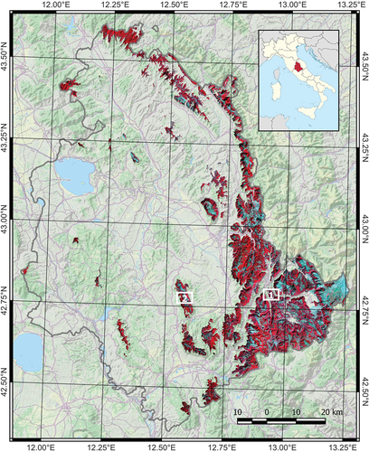
The study area is located in the Umbria region of Italy (Figure 1). Since this study aims to detect changes in land cover, focusing on the secondary grasslands targeted by the LIFE IMAGINE, which are located in the region’s montane belt, the study area  was identified by selecting the regional areas with an elevation higher than or equal to 700 m a.s.l. The area (approximately 1713 km²) extends from the south to the north of the eastern portion of the region and covers the Umbrian side of the Umbria-Marche Apennines. The area includes the east side of Vettore mountain’s complex, which has a maximum altitude of 2437 m (Cima del Redentore and Cima del Lago). The average altitude of the study area is 965 m.

Figure 1. Location of Umbria in Italy (red polygon in the inset). The study area is shown in Landsat 8 composite infrared together with the boundaries of the Umbria region and the OCM Landscape layer in the background. White rectangles indicate the locations of the areas chosen to show the classification results in detail.

The Umbrian Natura 2000 network includes 102 sites: 5 SPAs and 97 SACs. The network protects 41 habitats of the Habitats Directive Annex I, i.e. habitats of community interest, of which 11 are defined as priorities due to their particular importance, 143 animal species (4 priority), and eight plant species (1 priority). The study area includes 65 sites of the Umbrian Natura 2000 network, containing the vast majority of the regional grassland habitats, with a total protected area of approximately 540 km². Secondary grassland habitats (Annex I types 6210 and 6230*, Directive 92/43/EEC) are very relevant to the Umbrian Natura 2000 network, especially within the sites falling along the Apennine ridge. The Habitat type 6210 consists of semi-natural dry grasslands and scrubland facies on calcareous substrates. It includes a wide range of grassland communities generally assigned to the phytosociological class Festuco valesiacae-Brometea erecti Br.-Bl. & Tüxen ex Br.-Bl. 1949 (Biondi and Blasi 2015). It is considered of priority importance when hosting remarkable orchid sites (Annex I, Directive 92/43/EEC). The habitat type 6230* consists of closed, dry or mesophile, perennial, acidophilic Nardus grasslands developed on siliceous substrates in mountain areas, including plant communities assigned for the central and Southern Italian peninsula to the phytosociological class Ranunculo pollinensis-Nardion strictae Bonin 1972 (Biondi and Blasi 2015). Relevant occurrences of four plant species of community interest (Himantoglossum adriaticum H. Baumann, Ionopsidium savianum (Caruel) Ball ex Arcang., Iris marsica I.Ricci & Colas., Klasea lycopifolia (Vill.) Á.Löve & D.Löve, nomenclature according to the Portal to the Flora of Italy (Portal to the Flora of Italy, 2023), related to grassland habitats and listed in Annexes II and IV of the Habitats Directive are also present in the study area.

2.2 Methodological framework

We developed a diachronic land cover classification in GEE to assess the main changes in the study areas between 2000, 2010, and 2020, focusing on grasslands’ transformations. The Landsat data collection was selected as the primary source of spatial information since it is the only remote sensing dataset covering the whole analysis period. Considering the research objectives, the Landsat data characteristics, and the main land cover categories composing the landscape mosaic of the study area, we identified five land cover classes for the diachronic land cover analysis (woodland, shrubland, grassland, cropland, and sparse/no vegetation) (Table 1). The methodological workflow was defined according to a typical LULC change analysis and forecasting process, including a) data composition and preprocessing, b) image classification, c) accuracy assessment, d) land cover change and forecast analysis (Figure 2).

Figure 2. Methodological workflow of the research.

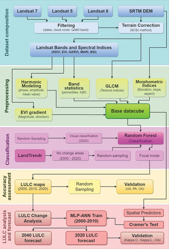
Table 1. Selected LULC classes, codes, and descriptions.

LULC Class	Code	Description
Woodland	1	Forest vegetation, dominated by different tree species.
Shrubland	2	Shrubs and scrublands (usually dominated by brooms, juniper, blackthorn, and hawthorn).
Grassland	3	Grassland vegetation, predominantly comprised of grasses, forbs, and small shrubs in variable proportion, ranging from dense and continuous to sparse and discontinuous, including both primary and semi-natural secondary grasslands (including habitat types 6210 and 6230*, Annex I, Directive 92/43/EEC).
Cropland	4	Agricultural mosaic mainly composed of annual crops.
Sparse/No Vegetation	5	Areas characterized by very sparse and fragmented vegetation cover, with a remarkable presence of rocky substrate; persistently non-vegetated areas characterized by bare soil; built-up areas.

We integrated various data preprocessing steps to increase Landsat data informative content and applied a state-of-the-art ML classifier to improve the classification results in GEE. We integrated the LandTrendr algorithm to automatically generate training datasets for 2000 and 2010 to reduce the time required for ML training sample collection drastically. This choice required additional and independent accuracy analysis steps. The land cover classification outputs provided an initial period to train the LULC forecasting model (2000–2010) and a validation period (2010–2020) to assess the predictive ability of the MLP-ANN model used for the 2040 forecast. In the following paragraphs, the methodological steps are described in detail.

2.3 Data composition and preprocessing

Generating the composite dataset is a pivotal step in any LULC classification process. To obtain the base data-cube for the ML classification and improve the information content of Landsat data, we developed an enhanced map composition in GEE, including various steps: 1) time filtering and cloud filtering, 2) topographic correction, 3) spectral indices calculation, 4) harmonic modeling, 5) band and index statistics calculation, 6) GLCM textural analysis, 7) EVI gradient analysis and slope calculation, and 8) morphological indices calculation. Even though the use of all these input features can appear as a heavy strategy, the utilization of GEE is highly effective in achieving the desired base data-cube.

We used the atmospherically corrected Surface Reflectance (SR) data from Landsat 7 (L7), Landsat 5 (L5), and Landsat 8 (L8), accessible through GEE. As previously performed in other studies (Tassi et al. 2021; Xie et al. 2019), to obtain a more robust cloud-free composite image for subsequent classification, we filtered the L7, L5, and L8 datasets using a cloud-coverage threshold of 20%, covering a substantially broad time span, in this case, three years for each period under investigation (104 L7 images from 1999 to 2001, 108 L5 images from 2009 to 2011, and 158 L8 images from 2019 to 2021). On the filtered datasets, we utilized the “pixel_qa” band to implement an initial filtering procedure on the derived dataset, effectively masking the majority of pixels occupied by dense clouds, cirrus clouds, and their associated on-ground shadows (Nyland et al. 2018).

A topographic correction in mountainous areas is ordinarily necessary to reduce the topographic effect before calculating spectral indices and image classification (Richter, Kellenberger, and Kaufmann 2009). To this aim, using the 30 m Shuttle Radar Topography Mission Digital Elevation Model (SRTM DEM), the Sun-Canopy-Sensor + C (SCSc) correction method was implemented (Soenen, Peddle, and Coburn 2005; Vanonckelen et al. 2014), which has demonstrated successful application in other research (Belcore, Piras, and Wozniak 2020; Shepherd and Dymond 2003) and is already integrated in GEE (Burns and Macander, n.d.). To fix some noise and anomalies detected in the initial SCSc results, we applied a 2-cell radius low-pass filter to the DEM as performed in previous studies (Hurni, Van Den Hoek, and Fox 2019).

Generally, adding spectral indices improves the final classification (Capolupo, Monterisi, and Tarantino 2020; Singh et al. 2016). In this regard, we computed five spectral indices for each image (Table 2). To improve the distinction between different types of vegetation cover, we calculated the Normalized Difference Vegetation Index (NDVI), Enhanced Vegetation Index (EVI), Modified Anthocyanin Reflectance Index (MARI), and Green Atmospherically Resistant Vegetation Index (GARVI). The NDVI is a widely used vegetation index that directly assesses vegetation health. Its normalized difference formulation and reliance on chlorophyll absorption and reflectance regions contribute to its robustness across various conditions (Singh et al. 2016). EVI is a more reliable biomass proxy than NDVI in areas with high soil exposure and dense vegetation due to its higher resilience to saturation, resistance to soil effects, and atmospheric contamination (Huete et al. 2002; Matsushita et al. 2007). MARI was employed to assess the content of red pigments (anthocyanins) in vegetation (Gitelson, Keydan, and Merzlyak 2006). GARVI is minimally affected by atmospheric conditions and remains sensitive to a wide range of chlorophyll-a concentrations (Gitelson, Kaufman, and Merzlyak 1996; Tassi et al. 2021). Additionally, BSI was used to better discriminate bare soil from other land cover types (Chen et al. 2004; Diek et al. 2017).

Table 2. Spectral indices and related formulas.

Index	Formula	Authors
NDVI	$\frac{NIR-RED\hspace{0.17em}}{NIR+RED}$	(Rouse et al. 1973)
EVI	$2.5\times \frac{NIR-RED}{NIR+\left(6\times RED\right)+\left(7.5\times BLUE\right)+1}$	(Huete et al. 2002)
GARVI	$\frac{NIR-\left(GREEN-\left(BLUE-RED\right)\right)}{NIR-\left(GREEN+\left(BLUE-RED\right)\right)}$	(Gitelson, Kaufman, and Merzlyak 1996)
MARI	$\left(\frac{1}{GREEN}-\frac{1}{RED}\right)\times NIR$	(Gitelson, Keydan, and Merzlyak 2006)
BSI	$\frac{\left(SWIR1+RED\right)-\left(NIR+BLUE\right)}{\left(SWIR1+RED\right)+\left(NIR+BLUE\right)}$	(Rikimaru, Roy, and Miyatake 2002)

We developed the harmonic data modeling on the three-year Landsat datasets using the approach and the related GEE script proposed by Clinton (Clinton 2016). Following this approach, a periodic signal, such as seasonal or phenological variations, can be modeled as a combination of simple waves or “harmonics” using linear combinations of sine and cosine functions (Shumway and Stoffer 2017). By using this technique, it is possible to adjust the number of harmonics and obtain “smoothed” values that filter out noise caused by outliers or data that may have been affected by adverse atmospheric conditions (Valderrama-Landeros et al. 2021). Three harmonic components (phase, amplitude, and mean value) were derived in GEE from the Landsat NDVI time series.

To improve the quantity of available information, we calculated three percentiles (10^th, 50^th, 90^th) and the interquartile range (IQR) for all the available bands and indices for the three time periods. These additional features have already been used to improve land cover classification accuracy (Hansen et al. 2014; Van De Kerchove et al. 2021).

GLCM (Gray-Level Co-occurrence Matrix) is a matrix representation of the frequency of occurrence of pairs of pixel values in a grayscale image (Mohanaiah, Sathyanarayana, and Gurukumar 2013). By analyzing the statistical properties of the GLCM, various texture features can be extracted, such as contrast, homogeneity, entropy, and energy. In order to produce 18 different textural indices through GLCM textural analysis in GEE, an 8-bit image with gray-level values is required as input. The algorithm calculates statistical data on texture characteristics by analyzing the distribution of intensity combinations observed at specified positions relative to one another in the image up to the second order (Mohanaiah, Sathyanarayana, and Gurukumar 2013). The input for the GLCM step was generated by applying a weighted linear combination (Equation 1), typically used for RGB image to grayscale conversion, to the median values of B3, B4, and B5 bands (Tassi et al. 2021; Vizzari 2022) as follows:

(1) $\mathrm{G}\mathrm{r}\mathrm{a}\mathrm{y}=\left(0.3\times \mathrm{B}5\right)+\left(0.59\times \mathrm{B}4\right)+\left(0.11\times \mathrm{B}3\right)$(1)

We selected nine textural indices (Table 3), also considering what was suggested by Hall-Beyer (2017).

Table 3. Textural indices calculated using GLCM (gray-level Co-occurrence matrix).

CODE	GEE CODE	Textural index description
T1	ASM	Angular Second Moment: estimates the number of repeated pairs in the image
T2	CONTR	Contrast: estimates the contrast within an image
T3	CORR	Correlation: estimates the correlation between pairs of pixels in the image
T4	VAR	Variance: estimates the extent of dispersion in the distribution of gray-levels in the image
T5	IDM	Inverse Difference Moment: estimates the homogeneity of the image
T6	SAVG	Sum Average: calculates the mean of the gray level sum distribution of the image
T7	SVAR	Sum Variance: estimates the dispersion (regarding the mean) of the gray-level sum distribution of the image
T8	SENT	Sum Entropy: estimates the randomness of the gray-level sum distribution of the image
T9	ENT	Entropy: estimates the randomness of the gray-levels distribution of the image

The gradient of an image at a particular point is a vector pointing in the direction of the most rapid change in intensity, and the length of the vector corresponds to the rate of change (Jin et al. 2012). Using the median EVI index and the proper GEE functions, we calculated specific, additional spatial indices: the gradient components (magnitude and direction), the local standard deviation (using a circular three-cells-radius kernel), and the slope of the index to improve the available information.

Morphometric indices (elevation, slope, aspect) were calculated from the Shuttle Radar Topography Mission Digital Elevation Model (SRTM DEM) to consider the complex morphological features of the study area and improve the classification accuracy as proposed by previous studies (Fahsi et al. 2000; Vogelmann, Sohl, and Howard 1998).

2.4 Land cover classification and accuracy assessment

We performed the land cover classification for the three datasets using the Random Forest (RF) machine learning classifier, aiming to discretize five classes: woodland, shrubland, grassland, cropland, and sparse/no vegetation (Table 1). We chose the RF algorithm among various ML classifiers due to its ability to handle large datasets with high dimensionality, its robustness against overfitting, and its capacity to provide feature importance, offering a good balance between accuracy and interpretability (Breiman 2001; Tassi and Vizzari 2020).

To train the RF classifier, we collected 1070 randomly distributed points for 2020, with a reciprocal minimum distance of 100 m, to reduce spatial autocorrelation (Figure 1 SM). These points were classified in QGIS (v. 3.22.11), visually integrating information from high-resolution 2020 orthophotos. RF employs the technique of bootstrap aggregation (bagging) to build multiple decision trees (DT) to combine the results, employing a majority voting method to enhance prediction accuracy (Gislason, Benediktsson, and Sveinsson 2006). RF algorithm in GEE allows for the assessment of the importance of the variables through the Gini index and the OOB (Out Of Bag) subset, which is helpful for multi-source studies (Rodriguez-Galiano et al. 2012a).

When high data dimensionality, the RF can be applied only to variables identified as most important in the first application (Rodriguez-Galiano et al. 2012a). Therefore, given the large number of bands in our dataset, we selected the most important ones by sorting them according to their importance, making several attempts to exclude some of them, and monitoring the accuracy of the classification provided by the OOB errors. Similarly, we tested the model’s output sensitivity to the most critical hyperparameters: the number of trees (“numberOfTrees”) and the number of variables per split (“variablesPerSplit”). These parameters were set to 350 and the square root of the number of variables (the default value in GEE). Also, in this case, these settings were determined by analyzing out-of-bag (OOB) errors obtained from numerous classification attempts.

Once the 2020 land cover classification was obtained, we used the LandTrendr (LT) algorithm to obtain RF training datasets for 2000 and 2010. In this application, we used LT to identify no-change areas over the last 20 years (2000–2020). LT is low computational intensive and can be applied relatively easily (Pasquarella et al. 2022). It works by first converting the raw satellite imagery into a series of spectral indices that can be used to quantify vegetation health and density. LandTrendr algorithm uses a linear regression model to fit a curve to the vegetation index time-series data for each pixel in the study area. The algorithm then identifies any significant deviations from the fitted curve, which are assumed to be caused by land cover change. Then, LT uses a cluster analysis technique to group similar change patterns, which can help to distinguish between different types of land cover change (e.g. natural disturbances vs. human-caused land use changes). Since our classification was based on five classes referring to different vegetation types, we used EVI as the vegetation index for analyzing changes with LT. Among the various vegetation indices available in LandTrendr, we opted for EVI because it is well-known for its higher resilience to saturation and resistance to soil effects and atmospheric contamination compared to other vegetation indices (Huete et al. 2002; Matsushita et al. 2007). To calculate the average annual EVI time-series in LT, we selected the June 20^th to September 20^th period as the most representative of the vegetation status in the study area. No gap was present in the annual EVI time-series. We adopted LT’s optimized standard settings to calculate two layers of gain and loss in the time series of EVI in GEE (Table 1 S.M.). Using these layers, exported to GEE assets, we created a mask identifying no-change areas with a magnitude of change (gain or loss) of less than 0.02 of the EVI value. These no-change areas in EVI over the 1999–2021 period were considered stable and belonging to the same land cover class over the entire time range. In these areas, a new training dataset for the classifier of 1950 random samples was generated (Figure 1 SM). These samples were classified by assigning them to the class detected in 2020 and used as RF training samples to generate LULC maps of 2000 and 2010. This approach prevented us from performing a new classification of the RF training dataset for 2000 and 2010. Therefore, the LT integration in the proposed methodology framework is chosen because it is cost-effective and customizable. It reduces the time to produce multi-year LULC maps by collecting automatic training data within the no-change areas.

We obtained land cover maps for 2000 and 2010, developing two RF models using the LT-derived training datasets and the data cubes composed for the same years. We developed the feature selection step and the hyperparameters definition (“numberOfTrees” and “variablesPerSplit”) for the RF models as previously done for the 2020 model. A final focal mode using a two-pixels radius was performed on the three land cover datasets to reduce the salt-and-pepper effect (Tassi et al. 2021). Considering the limited and variable relevance of only some GLCM features, we statistically assessed the benefits of incorporating these features through a McNemar test comparing the classification results obtained for the three years with and without GLCM features.

Finally, we assessed the accuracy for all three classifications using the AcATaMa plug-in of QGIS (Llano 2022). For this purpose, using an area-based proportion, a new independent, stratified random sampling was generated for each LULC map with a reciprocal minimum distance of 100 m and a minimum number of 8 neighboring pixels of the same class. The 96% confidence interval (CI) with a 0.004 margin error was adopted for defining the initial sample numerosity. Following Olofsson et al. (2014), we shifted the allocation slightly from proportional by increasing the number of samples in the rare classes to a minimum of 50. Thus, 620 points were generated and allocated to the five classes. The AcATaMa plug-in provided some specific accuracy metrics for assessing the classification: the overall (OA), user’s (UA), and producer’s (PA) accuracy for each class (Foody 2002) was conducted using the same QGIS plug-in and method implemented for the accuracy assessment of 2020. For this purpose, we used high-resolution orthophotos from 2000 and 2010 as ground truth data.

2.5 LULC change analysis

This analysis used the post-classification image comparison technique (Lu et al. 2004). Post-classification change analysis is usually adopted to reduce the external impact of atmospheric and environmental differences between the multi-temporal image (Lu et al. 2004). The classified images were compared in two periods, i.e., 2000–2010 and 2010–2020. In this step, we included logical restrictions to land cover change processes based on the original land cover. We did not permit changes from woodland to other land cover classes considering that the decrease of woodland is extremely rare in the area and time of analysis and typically not permanent. To support this choice, we used LandTrendr to measure the magnitude of disturbances in the woodland-to-other transitions and the no-change woodland areas in the two analysis periods. We computed an Analysis of Variance (ANOVA) to assess if their differences were significant. The magnitude of change was significantly higher in wood-to-other transitions than in no-change woodland areas [2000–2010: F(3, 908) = 74.93, p < 2e-16; 2010–2020: F(3, 871) = 45.51, p < 2e-16]. Thus, we excluded the hypothesis of misclassification and the loss of woodland in our study area was associated with a typically nonpermanent change due the tree-cutting practices. Hence, those areas were reclassified as woodland in the subsequent classification. On this basis, the LULC change analysis was developed for the whole study area and the Natura 2000 network sites included in the study area. Finally, we used Sankey diagrams to represent the inflows and outflows of each land-cover class over the two periods.

2.6 Future LULC forecast

We used the MOLUSCE (Modules for Land-Use Change Simulation) plug-in (NextGIS 2017) in QGIS (v. 2.18.26) to forecast the 2040 LULC. MOLUSCE is an open-source model for QGIS 2.0 and above to analyze temporal LULC changes and simulate the future land use with spatial variables (Muhammad et al. 2022). MOLUSCE is built with CA model, includes a transition probability matrix and incorporates a number of well-known algorithms: Multilayer Perceptron-Artificial Neural Networks (MLP-ANNs), Multi-Criteria Evaluation (MCE), Weights of Evidence (WoE) and Logistic Regression (LR). The MOLUSCE plug-in have been largely used in previous research for LULC changes forecasting (see e.g, Amgoth, Rani, and Jayakumar 2023; Aneesha Satya, Shashi, and Deva 2020; Ashaolu, Olorunfemi, and Ifabiyi 2019). This plug-in was chosen because of its simple interface, ease of use, QGIS integration, and free and open-source software development policy. For calibrating and modeling LULC changes, each model approach in MOLUSCE takes LULC change information and geographic factors as inputs (El-Tantawi et al. 2019; Kamaraj and Rangarajan 2022). The LULC change maps for the initial (2000) and final (2010) years were included in the first stage of the model. The pattern of 10-year LULC changes was determined using several variables identified as land cover drivers: morphometric indices (elevation, aspect, and slope; see 2.3), and Euclidean distance to urban areas, primary roads, grassland areas, shrublands area, and forest areas. All these variables were generated with a spatial resolution of 30 × 30 m. Furthermore, two climatic variables have been added, considered important land cover drivers: average annual temperature variation and average annual soil moisture variation. These variables were derived from ERA5-Land climate reanalysis data (Muñoz-Sabater et al. 2021), precisely the yearly “2-m air temperature” and “volumetric soil water layer 1” with a spatial resolution of 9 × 9 km were downloaded for each year between 2000 and 2010. Subsequently, the average annual variation was calculated for both variables.

A correlation test was conducted between LULC and the spatial driver using Cramer’s Coefficient (Abbas et al. 2021; Hakim et al. 2019; Muhammad et al. 2022). A high Cramer’s coefficient value (higher than 0.15) indicates that the potential explanatory variable helps explain land cover changes (Abbas et al. 2021; Hakim et al. 2019; Muhammad et al. 2022). Based on the 2000 and 2010 LULC maps, the explanatory variables, and the transition matrix, we projected the LULC for 2020 to validate the model’s predictive power. The MLP-ANN model was used in this study. Considering previous applications (Abbas et al. 2021; El-Tantawi et al. 2019; Kamaraj and Rangarajan 2022; Lukas, Melesse, and Kenea 2023; Muhammad et al. 2022) and after several tests, we set the parameters of the MLP-ANN method: neighborhood (1), learning rate (0.001), maximum iterations (100), hidden layer (12), and momentum (0.05). Finally, different statistics were measured while validating the actual and predicted 2020 LULC maps (Abbas et al. 2021; Kamaraj and Rangarajan 2022). The Kappa Overall is used to evaluate the overall success of the simulation, and Kappa Location is used to evaluate the ability of the simulation to identify location changes (Aneesha Satya, Shashi, and Deva 2020). Furthermore, the Percentage of Correctness (overall accuracy) of 0% indicates no agreement between actual and predicted maps, while 100% indicates perfect agreement (Aneesha Satya, Shashi, and Deva 2020). After obtaining satisfactory results from the model validation, the LULC map of 2040 was predicted using the same spatial variable combinations and MLP-ANN model by considering a 20-year step with three iterations. Finally, we developed the analysis of LULC change in 2040 for the entire study area and Natura 2000 areas as previously described.

3. Results

The base datacube for each period, obtained from combining all the bands and indices, comprises 63 features (Table 4).

Table 4. Bands and indices calculated for the composition of the base datacube.

Bands and indices	Number of bands	Codes/names
10^th, 50^th, 90^th percentiles and interquartile range of B1, B2, B3, B4, B5, B7 and NDVI, EVI, GARVI, MARI, BSI	44	Suffixes _p10, _p50, _p90, _iqr
Textural indices	9	T1 to T9
Harmonic components	3	‘phase,’ ‘magn,’ ‘val’
Elevation, slope, aspect	3	‘elevation,’ ‘slope,’ ‘aspect’
EVI slope, local standard deviation, gradient, and direction	4	‘slopevi,’ ‘sdloc,’ ‘grad,’ ‘dir’

The importance of features in the RF classification is quantified using the Gini index, which was suggested as an optimal measure of variable importance helpful for feature selection purposes (Menze et al. 2009). In this study, the importance of the features varies depending on the classification year, but some were prominent in all three periods. Out of the initial 63 features, considering the importance quantified by the RF classifiers and plotted in GEE, we selected 39 variables for 2000, 34 for 2010, and 38 for 2020. Figure 3 shows the importance of the variables involved in the classification.

Figure 3. Distribution of the importance scores of the variables used in the RF classification for (a) 2000, (b) 2010, and (c) 2020.

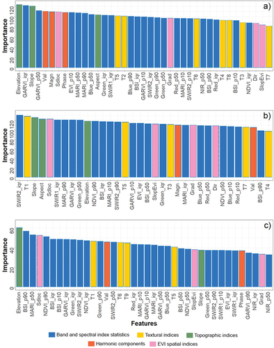
Concerning the morphological indices, excluding the aspect for 2020, they were relevant, with different importance, for all three classifications. In particular, the elevation was one of the most important. Some spectral indices' statistics were also relevant for all three classifications, particularly those derived from NDVI, GARVI, MARI, and BSI. Moreover, it is worth noting that somestatistics calculated for bands and indices (IQR, p10, p90) proved to be significantly more relevant than the traditional “median” (p50) in all three classifications, particularly for the spectral indices rather than the other bands (Figure 3). Out of all the percentile statistics, the IQR is selected in the most significant number of variables in all three classifications. The harmonic model components were important in all three classifications; “magn” and “val” were relevant for the 2000 and 2010 classifications, and “val” and “phase” were for the 2020 classification.

Regarding the textural indices, many of them assumed an apparent significance but different importance for all three classifications (Figure 3). T1 (Angular Second Moment) shows a high importance for the 2010 classification and a medium-high importance for the 2020 classification. Other relevant textural indices were T5 (Inverse Difference Moment), which was medium-highly important for all three classifications, and T6 (Sum Average) for the 2000 and 2020 classifications. However, the three McNemar tests aimed at assessing the relevance of the selected GLCM features showed that the slight increase in the average OA obtained using these metrics was not statistically significant (2020: p = 0.26; 2010: p = 0.33; 2000: p = 0.28).

Among the spatial indices derived from median EVI, the local standard deviation (”Sdloc”) was very relevant for all three classifications (Figure 3)The slope of the same index (”SlopeEVI”) was selected for all classifications but was less important . Concerning the gradient components, only “grad” was selected for all classifications and assumed various importance. “Dir” was selected but showed less relevance for the 2000 and 2010 classifications..

Regarding the LULC forecast for 2040 developed with the MOLUSCE QGIS plug-in, the spatial drivers selected through Cramer’s coefficient (C) were: elevation (C = 0.31), slope (C = 0.23), distance to urban areas (C = 0.19), distance to grassland areas (C = 0.29), distance to shrubland areas (C = 0.22), distance to forest areas (C = 0.50), and average annual increase in temperature (C = 0.16).

The overall classification accuracy (OA) obtained for each period was greater than 90% (Table 5). However, the user and producer accuracies of the individual classes varied over the three years (Table 5). The user and producer accuracies were fairly consistent. Notably, the shrubland class showed the lowest accuracy values (UA: 0.69–0.73; PA: 0.58–0.76).

Table 5. Accuracy metrics of LULC classifications for each year (UA: User’s Accuracy; PA: Producer’s accuracy).

LC Class	2000		2010		2020
	UA	PA	UA	PA	UA	PA
Woodland	0.92	0.99	0.9	0.99	0.95	0.98
Shrubland	0.69	0.69	0.73	0.58	0.73	0.76
Grassland	0.99	0.71	0.94	0.7	0.95	0.82
Cropland	0.94	0.8	1	0.9	0.92	0.78
Sparse/No Vegetation	0.9	1	0.94	0.88	0.82	0.9
OA	0.90 ± 0.012		0.90 ± 0.012		0.92 ± 0.011

Regarding the LULC simulation, the validation between actual and predicted 2020 LULC resulted in a Kappa Overall = 0.772, Kappa Location = 0.869, and 90.837% overall accuracy. Based on these results, we proceeded with the 2040 LULC forecast.

Concerning the change analysis, it should be noted that our study area is located at medium-high altitudes (700–2437 m a.s.l.), and it comprises mainly natural and semi-natural habitats, where forests and grasslands were the most represented land cover types (Table 6). However, while forests increased (10.2%) over the last 20 years, the area covered by grasslands decreased (−18.1%). For both classes, the most significant changes occurred between 2000 and 2010, followed by 10 years of greater stability (Table 6). Forest increases were mainly represented by spontaneous transitional flows due to natural dynamic processes in shrubland areas, particularly in the first 10 years (70 km² between 2000–2010; Figure 4). On the other hand, resulting from natural dynamic processes as well, grasslands suffered the loss of large areas due to conversion to shrubs (about 20 km² each decade) or forests (26 km² between 2000–2010). (Figure 4; example in Figure 5, full output maps are reported in Figure 2 SM). Shrublands experienced inflows from grasslands and outflows to forests (Figure 4). However, net of these transitions, the area covered by shrublands decreased (−32.6%) throughout the last 20 years (Table 6). Agricultural areas increased in the first 10 years, then decreased sharply between 2010–2020. Non-vegetated and eroded areas decreased in the first 10 years and then increased to the initial levels between 2010–2020. According to the forecast, forests are expected to expand even more, potentially reaching approximately 1356 km² by the year 2040 (Table 6). This expansion would cover around 80% of the entire study area. On the other hand, both shrublands and grasslands are projected to decrease in the future. The decline in shrublands is estimated to be more significant, with an approximate decrease of 41.5%. In contrast, grasslands are expected to experience a comparatively smaller decline of around 15.6% (Table 6; see example in Figure 5, full output maps are reported in Figure 2 SM). Additionally, sparse vegetation areas, previously subject to minor fluctuations, are expected to undergo a considerably more significant decline of approximately 43.9%. According to the forecast, croplands are expected to grow substantially (+43.1%).

Figure 4. Sankey’s diagram showing the main transition flows (greater than 5 km²) between the five land-cover classes in the study area between 2000–2010, 2010–2020 and 2020–2040.

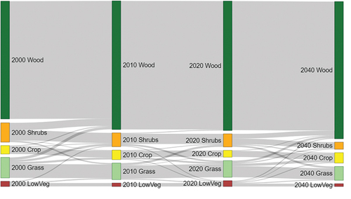
Figure 5. Land cover maps of 2000, 2010, 2020, and 2040 in two exemplifying areas. The scale and the north sign are indicated in the final image of both areas. The full maps, and a comparison with orthophoto and a global land cover product are provided in the supplementary materials.

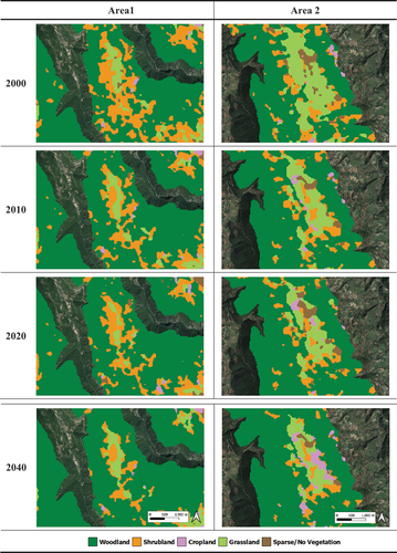
Table 6. Area of land cover classes (km²) in three different years (2000, 2010, 2020) and the increase/decrease percentage over 20 years (2000–2020) for the entire study area and the Natura2000 sites. The potential area of land cover classes (km²) and percentage of increase/decrease are also shown for the 2040 forecast.

LC Class	Code	Study Area						Natura2000
		2000	2010	2020	2040	2000–2020%)	2020–2040%)	2000	2010	2020	2040	2000–2020%)	2020–2040%)
Woodland	1	1164	1271	1283	1356	+10.2	+5.7	332	357	359	381	+8.1	+6.1
Shrubland	2	193	137	130	76	−32.6	−41.5	44	34	34	16	−22.7	−52.9
Cropland	3	91	96	72	103	−20.9	+43.1	20	24	19	28	−5	+47.4
Grassland	4	204	165	167	141	−18.1	−15.6	112	103	98	96	−12.5	−2.0
Sparse/No Veg.	5	56	40	57	32	+1.8	−43.9	31	23	30	20	−3.2	−33.3

Within Natura 2000 areas, forests and grasslands are the dominant land cover classes. For the Natura 2000 sites, the patterns of increase/decrease in class areas were consistent with those found at the study area level (Table 6). However, positive and negative changes in the last 20 years affected smaller portions of the areas within the Natura 2000 sites compared to the overall results obtained for the entire study area, outlining a picture characterized by a lower intensity of land use transformation inside the Natura 2000 Network. The only class with a clearly different pattern was class 5, although shifting around very low rates of change (Table 6). The forecast for 2040 suggests a less negative trend for grasslands within Natura 2000 areas, indicating a potential marginal decrease (−2%) compared to the 12.5% decrease observed between 2000–2020. On the other hand, significant changes are projected for shrublands and sparse vegetation areas. A substantial intensification of the observed patterns from previous years shows a projected decline of 53% and 33%, respectively (Table 6). Notably, even within Natura 2000 sites, sparse vegetation areas will no longer experience minor fluctuations but rather more significant changes in the future, reflecting the trends observed outside protected areas. Also, according to the forecast, croplands are expected to increase considerably (+47.4%) in these areas.

4. Discussion

4.1 Land cover analysis and forecasting in GEE

In this application, the utilization of GEE proved to be highly effective in achieving the desired Landsat data composition. Adding spectral indices and other ancillary data is not new in the Landsat data classification process (e.g. Rodriguez-Galiano et al. 2012b; Tassi et al. 2021). However, unlike previous research with typical land cover classification, we successfully developed an “enhanced” map composition in GEE, integrating the harmonic model approaches and other information such as textural indices, topographic and vegetation gradients, and additional statistics derived from Landsat data. Despite using medium-resolution data (i.e. Landsat 7/5/8), the high accuracy achieved for all three years (90–92%), together with the importance of these additional features in the RF classifications, showed that increasing the information content of Landsat data through such enhanced map composition was efficient for our classifications.

Morphological indices (elevation, slope, and aspect), also considering their role in influencing vegetation development and differentiation, were relevant for all the classifications. This result confirms what is suggested in previous studies (e.g. Fahsi et al. 2000 Strahler, Logan, and Bryant 1978; Hutchinson 1982). According to our results, Landsat composite bands and indices derived using percentiles (10^th, 50^th, 90^th, and IQR) were crucial for all the classifications. This evidence confirms previous studies suggesting that band and spectral index statistics can improve the accuracy of land cover classification (Griffiths, Jakimow, and Hostert 2018; Nill et al. 2022; Van De Kerchove et al. 2021) and suggests that these additional indices are frequently more important than the simple, more frequently used median.

GLCM textural analysis applied to Landsat data, despite the non-ideal resolution for this kind of analysis, provided relevant features for the RF classifications. This evidence confirms what was highlighted in previous studies about the relevance of these features for Landsat data RF classification (Jin et al. 2018; Lu, Batistella, and Moran 2007; Tassi et al. 2021). However, the McNemar tests showed that, despite the importance of some of them in the RF classification, adding these features was not statistically significant for improving accuracy results. Therefore, in this application, the image smoothing generated averaging data over three years could have decreased the significance of these features. Despite the limited spatial resolution of Landsat data, applying GLCM on single, representative images may increase the informative value of these features.

Compared to the similar approach used for obtaining the GLC_FCS30 (Zhang et al. 2021), the method developed in this study proposes an enhanced Landsat data composition which includes harmonic modeling and vegetation gradient analysis in addition to topographic, textural, and statistical features. Our results highlight the relevance of harmonic models’ seasonal features for the three land cover classifications. This evidence agrees with previous studies (e.g. Esch et al. 2014; Liu et al. 2016; Senf et al. 2015). The EVI local standard deviation (SD), slope calculation, and gradient analysis based on the same index provided additional relevant features according to the RF classifications. Regarding the SD, our results confirm a previous study where the NDVI SD was used to improve land cover classification accuracy (Becker et al. 2021). The image gradient analysis was already used for edge-detection preliminarily to image classification (Oram, McWilliams, and Stolzenbach 2008). However, to our knowledge, the direct use of the gradient metrics (magnitude and direction) and the EVI slope index appears new in land cover classification.

While LandTrendr (LT) has already been used in prior research for supporting land cover classification (Mugiraneza, Nascetti, and Ban 2020), to our best knowledge, our research is the first to integrate this algorithm in LULC classification to derive training samples within no-change areas automatically. The application of LT allowed us to achieve high classification accuracy while saving the time required to manually classify the RF training points for 2000 and 2010. These results, even though obtained in a low anthropized study area, suggest that LT, beyond its usual application, could effectively reduce the time needed to produce multi-year land cover maps.

The utilization of GEE scripts developed in this research in other study areas, also thanks to GEE versatility, seems relatively straightforward, provided that the Landsat data is available and free from issues not addressed in this study, such as the L7 SLC-off problem, that should be appropriately addressed. The accuracy assessment of land cover maps conducted in this study, based on the AcATaMa QGIS plug-in, could be somewhat challenging. However, this step was implemented to provide an additional assessment beyond what could be typically implemented in the random forest classification using training and validation data.

Despite the high overall accuracy achieved for the 2000, 2010, and 2020 land cover maps, it is essential to mention that the shrub class emerged as the most complex to differentiate. Shrublands had a lower accuracy (user and producer) than the other classes, particularly in 2000 and 2010. Typically, shrublands consist of a variety of plant species, which may encompass diverse shrubs, trees, or herbs and develop various structural and spectral features (Oddi et al. 2021; Suess et al. 2018). As highlighted in other studies, mapping classes that comprise a blend of land cover and plant functional types posed a notable challenge, mainly due to the resolution of the Landsat data whereby 30 m pixels usually comprise a mixture of at least two land cover types (Dong et al. 2019; Friedl et al. 2022). Although Landsat images have a finer spatial resolution than other satellites (e.g. MODIS), it is essential to consider that, even if we assign a single label to each pixel, there are only a limited number of pixels that are homogeneous concerning the composition of the land cover, even at a resolution of 30 m (Friedl et al. 2022). This issue becomes more relevant in fragmented landscapes like the Italian and Umbrian ones. Nevertheless, as our study covered a broad period, Landsat remains the available remote sensing data source with the best spatial resolution.

Additionally, the forecasting method employed in this study, along with the selection of spatial drivers to predict LULC change, demonstrated high efficiency compared to other studies (Amgoth, Rani, and Jayakumar 2023; Aneesha Satya, Shashi, and Deva 2020; Hakim et al. 2019; Kamaraj and Rangarajan 2022; Lukas, Melesse, and Kenea 2023). The validation step proved the results’ reliability, showing consistency between the actual and predicted 2020 LULC. However, it is essential to note that our prediction was based on historical trends observed in the study area between 2000 and 2010. Given that the most significant land cover changes occurred from 2000 through 2010, there is a potential for the predicted changes between 2020 and 2040 to be exacerbated despite the good results obtained from validating the MLP-ANN model with the simulated 2020 LULC map. The forecasted substantial growth of croplands, which seems unrealistic considering the ongoing socio-economic dynamics, could be related to this issue. It is worth emphasizing that our future LULC modeling and prediction only incorporated physical and climatic factors. To further enhance the analysis, future studies should consider incorporating socioeconomic factors (Abbas et al. 2021). Overall, the forecast suggests a shift in the grassland landscape of the Umbria region toward more forested and cropland areas at the expense of shrublands, grasslands, and sparse vegetation. This could have significant implications for local ecosystems, biodiversity, climate, and human activities. In particular, the significant expansion of forests in the grassland landscape of Umbria by 2040 could imply an increase in carbon sequestration and potential changes in local climate conditions. Both shrublands and grasslands are expected to decrease, with shrublands experiencing a more significant decline. This could lead to habitat loss for certain species, potential changes in local ecosystems, and biodiversity loss.

Although, to our knowledge, local validation of GLC finer resolution datasets in our study area has yet to be conducted, comparing the accuracy metrics of these datasets with our results could offer valuable insights. In general, our land cover maps demonstrated significantly higher accuracy performance, averaging 90.7%, in contrast to 82.5% of GLC_FCS30–2015, 59.1% of FROM_GLC-2015, and 75.9% of GlobeLand30–2010 (Table 2 S.M). Regarding the accuracy of land cover classes, our results generally outperformed these datasets in terms of producer’s and user’s accuracies, except for croplands, which were slightly better classified by GLC_FCS30–2015 and GlobeLand30–2010 (with an approximately 5% higher producer’s accuracy). Notably, this research achieved remarkably superior results for Grasslands’ User’s Accuracy compared to other datasets (GLC_FCS30–2015 by + 27%, FROM_GLC-2015 by + 70%, GlobeLand30–2010 by + 60%). A visual comparison with the corresponding GLC_FCS30 datasets shows the focal filter’s effect on this research’s outputs in reducing the salt-and-pepper effect (Figures 3 and 4 S.M.). The same comparison confirms the improved performance of the outputs obtained in this research for grasslands and shrublands.

4.2 Grasslands’ dynamics in the study area

Our study contributes to the ongoing efforts to enhance the effectiveness of remote sensing-based approaches for identifying critical grassland regions. The proposed methodology allowed us to map the medium-high-altitude grassland areas in Umbria and enabled the identification of crucial transformation phenomena responsible for grassland degradation. These phenomena encompass the encroachment of shrubs and woody plants and the reduction of biomass resulting from erosion over 20 years in the past and an additional 10 years into the future. Our findings indicate that shrubs/woody plant invasion into grassland areas occurred in our study area. In the span of two decades, from 2000 to 2020, there was a significant decline of 18% in the extent of grasslands, primarily attributed to their conversion into more densely vegetated land covers (shrubland and forest). This transition toward woody vegetation is further supported by the notable expansion of forest areas, which increased by 10.2% during the same period. This trend is projected to persist over the next 10 years (2040), with forests expected to gain an additional 73 km² of coverage while grasslands potentially lose another 14 km². Our findings highlight that the expansion of the forest has been driven by the conversion of shrublands and to a lesser extent of grasslands. However, overall, the shrubland surface has decreased over the same time, as a larger area has been converted from shrubland to forest than grassland to shrubland.

It is important to note that the most major changes in land cover occurred between 2000–2010. In contrast, the subsequent decade was characterized by fluctuations rather than significant changes, particularly for forests, shrublands, and grasslands. However, the overall 20-year overview revealed the occurrence of woody plant encroachment, which has already been found in similar habitats (Gartzia, Alados, and Pérez-Cabello 2014; Komac et al. 2013; Malatesta et al. 2019; Saintilan and Rogers 2015). As observed in other areas, the progressive evolution involves the intrusion by native shrubs into grasslands, followed by the natural afforestation of shrub areas (Gartzia, Alados, and Pérez-Cabello 2014). In our study area, two factors could explain the reduction in shrub cover despite the transition from grasslands and the significant increase in forest area. First, it has been shown that proximity to a wooded area is one relevant factor associated with the conversion of grassland to shrubland or forest (Gartzia, Alados, and Pérez-Cabello 2014). In addition, once the shrub encroachment process is established, it is self-amplifying with positive feedback mechanisms in which the encroachment is even stronger in areas where woody vegetation is already present (Brandt et al. 2013). Additionally, the effect of climate change, particularly the increase in CO₂, should also be mentioned. Rising levels of atmospheric CO₂ promote the growth of woody plants over grassland habitats, as already observed by several studies (e.g. Archer et al. 2017; Devine et al. 2017; Saintilan and Rogers 2015; Scheiter and Higgins 2009; Soubry and Guo 2022; Venter, Cramer, and Hawkins 2018), and climate change simulations predict a severe shift toward habitats globally dominated by shrubs and woody plants in the future (Archer et al. 2017; Scheiter and Higgins 2009).

When analyzing land-use changes within Natura 2000 areas of the study area, we observed consistent trends with those observed outside these areas over the last two decades. While the process of vegetation densification is also happening within Natura 2000 sites, as seen in our study and others (Calaciura and Spinelli 2008), it is crucial to note that the proportion of surfaces undergoing significant changes within these areas was smaller compared to the general trend outside the protected areas network. These results suggest that the Directives governing the management of Natura 2000 areas have been somewhat effective. Moreover, there are promising indications of a substantial slowdown in the future decrease of grassland coverage within these protected zones. However, more actions are needed to address the challenges within these sites and to ensure their sustainability in the long run (Calaciura and Spinelli 2008; Carli et al. 2018).

4.3 Grasslands’ habitat degradation phenomena

Global estimates suggest that about half of the grassland on Earth has been degraded, although the extent and intensity of degradation vary significantly locally; among the primary cause of grassland degradation are anthropogenic activities (Bardgett et al. 2021). Two contrasting human-related factors are the major drivers in the loss of this habitat: on one side, increased disturbance caused by overgrazing reduces vegetation cover (Hilker et al. 2014) and, on the other, extensive land abandonment and cessation of grazing lead to shrubs and woody vegetation encroachment (Poschlod and WallisDeVries 2002). In mountain environments, land abandonment occurs where areas are more difficult to access or are left aside when less profitable. At the same time, easily accessible areas in the lowlands are characterized mainly by overexploitation (Sartorello et al. 2020). Several socioeconomic factors are responsible for land abandonment, including agricultural intensification and urbanization, which caused migration from rural areas and made traditional shepherding uneconomical (Poschlod and WallisDeVries 2002; Valkó et al. 2018). The abandonment of mountain grasslands triggers the vegetation successional processes. It results in a progressive change of plant community composition that, by altering the structure and functions of the ecosystem, leads to the loss of grasslands in favor of other land cover types (Estel et al. 2015; Gartzia, Alados, and Pérez-Cabello 2014; Malatesta et al. 2019; Oddi et al. 2021; Soubry and Guo 2022). Therefore, grassland maintenance directly depends on human activity and requires balanced grazing, as it contributes to maintaining the open mosaic and associated biodiversity that characterizes these habitat types (Poschlod and WallisDeVries 2002; Silva et al. 2019). In addition, future climate change will likely exacerbate grassland degradation by combining with human activities, causing increased woody plant encroachment in some areas and desertification in others (Anadón et al. 2014; Bardgett et al. 2021; Venter, Cramer, and Hawkins 2018). All these processes related to grassland degradation have been detected worldwide, including Europe (e.g. Gartzia, Alados, and Pérez-Cabello 2014; Malatesta et al. 2019; Sartorello et al. 2020).

It is well known that land abandonment or reduction in livestock pressure leads to changes in the community structure by favoring the process of shrub encroachment, thus favoring taller and denser vegetation types (Bardgett et al. 2021; Carli et al. 2018; Malatesta et al. 2019). Similar woody plant/shrub encroachment phenomena have been observed worldwide (Bardgett et al. 2021; Dong et al. 2019). The other phenomenon that causes grassland degradation is erosion, mainly due to overgrazing; however, our results did not show any alarming signals in this regard. Non-vegetated areas remained a small percentage of the total area over time and were only characterized by minor fluctuations. This suggests that the most relevant impacts on grasslands conservation are probably those determined by under-grazing and land abandonment, as already observed, especially in Europe (Calaciura and Spinelli 2008; Gartzia, Alados, and Pérez-Cabello 2014; Linnell et al. 2015; Poschlod and WallisDeVries 2002). Semi-natural grasslands have been shaped by centuries of human activity by clearing natural vegetation, such as forests, and by driving the natural grasslands’ floristic composition through traditional extensive livestock grazing (Bardgett et al. 2021; Poschlod and WallisDeVries 2002). In Europe, the cessation or decrease of livestock grazing associated with extensive land abandonment of semi-natural grasslands during the twentieth century has led to massive grassland loss (Bardgett et al. 2021; Poschlod and WallisDeVries 2002). Although they result from human activity, the European Union Habitats Directive requires the conservation of semi-natural grasslands (Gartzia, Alados, and Pérez-Cabello 2014; Linnell et al. 2015). Indeed, these types of grassland are of particularly high concern for conservation in Europe, as they serve as important reservoirs for biodiversity, being among the most species-rich plant communities in Europe (Calaciura and Spinelli 2008; Wilson et al. 2012) and have played a crucial role in the historical landscape, associated with high aesthetic and cultural heritage values (Bardgett et al. 2021; Linnell et al. 2015). Moreover, the loss of grassland habitats also reduces the rangeland area available for cattle and wildlife grazing, resulting in difficulties in maintaining forage quantity and quality for livestock that can lead to substantial global economic losses (Soubry and Guo 2022). One of the main challenges associated with ecological succession in the grasslands is that it cannot be naturally reversed, complicating efforts to address grassland conservation effectively (Gartzia, Alados, and Pérez-Cabello 2014; Komac et al. 2013). Human interventions, such as mechanical clearing, have not consistently yielded desired outcomes, and converting a woody plant system back to grassland is a more time-consuming process than the natural succession from grassland to shrubland (Gartzia, Alados, and Pérez-Cabello 2014). In conclusion, it can be inferred that areas affected by such phenomena can be restored as long as they are small and young. However, considering that the well-being of these habitats relies on the interplay between human actions and natural forces, it is imperative to promote sustainable practices that prioritize the conservation of such habitats. Encouraging traditional shepherding practices, which have become increasingly uneconomical over time (Poschlod and WallisDeVries 2002), can be a significant step toward achieving this goal.

5. Conclusions

This study developed a method for diachronic LULC classification in GEE through enhanced Landsat data composition, identification of no-change areas using the LandTrendr algorithm, and RF machine learning classification, achieving an overall accuracy greater than 90%. The enhanced dataset composition developed in GEE, including statistical image analysis, harmonic modeling, gradient, and GLCM analysis, provided additional information from the original Landsat data relevant for the RF classification and improved accuracy. However, in this specific application, the accuracy improvement related to adding the GLCM textural indices was not statistically significant.

The LandTrendr algorithm successfully simplified the diachronic land cover classification and change analysis, supporting automatic training data collection within the no-change areas. The study area includes highly variable grassland landscapes, and the proposed method based on LandTrendr was successfully tested on two different data sets collected in 2000 and 2010. Although they are from the same area, they exhibit different characteristics due to different environmental and management conditions. However, additional grassland sites should be analyzed using the proposed framework to provide additional data and further assess its robustness and general validity.

We investigated the grassland dynamics over the past two decades in Umbria, identifying shifting plant landscapes, affected on one side by shrubs/trees encroachment and on the other by reduced green biomass. Due to their mixed composition and particular spatial patterns, the shrublands area obtained lower user and producer accuracies, confirming that their classification is a great challenge using medium-resolution data. A specific analysis was developed supporting the analysis and management of habitats of European concern within Natura 2000 areas. These results may also help detect the areas where the conservation measures related to the Natura 2000 network have been more (or less) effective in grassland conservation. The outcomes of the spatiotemporal and projected LULC simulations could add relevant information for evaluating forecasted LULC changes. Specific spatially explicit management strategies could be defined to increase grassland conservation inside and outside Natura 2000 areas, and our results provide a scientific basis for making political decisions on managing these crucial habitats.

Acknowledgments

This research was developed within the LIFE Project “LIFE IMAGINE UMBRIA” LIFE19 IPE/IT/000015 funded by the European Union.

Disclosure statement

No potential conflict of interest was reported by the author(s).

Data availability statement

All remote sensing data used in the research are openly available in the USGS archives (https://earthexplorer.usgs.gov/) and within Google Earth Engine. The GEE codes developed in this research are available by emailing the authors upon any reasonable request.

Supplementary material

Supplemental data for this article can be accessed online at https://doi.org/10.1080/15481603.2024.2302221.

Additional information

Funding

This research was funded by the European Union - LIFE Project “LIFE IMAGINE UMBRIA” LIFE19 IPE/IT/000015.

References

- Abbas, Z., G. Yang, Y. Zhong, and Y. Zhao. 2021. “Spatiotemporal Change Analysis and Future Scenario of Lulc Using the CA-ANN Approach: A Case Study of the Greater Bay Area, China.” Land 10 (6): 584. https://doi.org/10.3390/land10060584.
- Amani, M., A. Ghorbanian, S. A. Ahmadi, M. Kakooei, A. Moghimi, S. M. Mirmazloumi, S. H. A. Moghaddam, et al. 2020. “Google Earth Engine Cloud Computing Platform for Remote Sensing Big Data Applications: A Comprehensive Review.” IEEE Journal of Selected Topics in Applied Earth Observations & Remote Sensing 13:5326–27. https://doi.org/10.1109/JSTARS.2020.3021052.
- Amgoth, A., H. P. Rani, and K. V. Jayakumar. 2023. Exploring LULC changes in Pakhal Lake area, Telangana, India using QGIS MOLUSCE plugin. Spatial Information Research 31 (4): 429–438. https://doi.org/10.1007/s41324-023-00509-1.
- Anadón, J. D., O. E. Sala, F. T. Maestre, and R. Bardgett. 2014. “Climate Change Will Increase Savannas at the Expense of Forests and Treeless Vegetation in Tropical and Subtropical Americas.” The Journal of Ecology 102 (6): 1363–1373. https://doi.org/10.1111/1365-2745.12325.
- Aneesha Satya, B., M. Shashi, and P. Deva. 2020. “Future Land Use Land Cover Scenario Simulation Using Open Source GIS for the City of Warangal, Telangana, India.” Applied Geomatics 12 (3): 281–290. https://doi.org/10.1007/s12518-020-00298-4.
- Archer, S. R., E. M. Andersen, K. I. Predick, S. Schwinning, R. J. Steidl, and S. R. Woods. 2017. “Woody Plant Encroachment: Causes and Consequences.” In Rangeland Systems: Processes, Management and Challenges, edited by D. D. Briske, 25–84. Cham: Springer.
- Ashaolu, E. D., J. F. Olorunfemi, and I. P. Ifabiyi. 2019. “Assessing the Spatio-Temporal Pattern of Land Use and Land Cover Changes in Osun Drainage Basin, Nigeria.” Journal of Environmental Geography 12 (1–2): 41–50. https://doi.org/10.2478/jengeo-2019-0005.
- Bardgett, R. D., J. M. Bullock, S. Lavorel, P. Manning, U. Schaffner, N. Ostle, M. Chomel, et al. 2021. “Combatting global grassland degradation.” Nature Reviews Earth and Environment 2 (10): 720–735. https://doi.org/10.1038/s43017-021-00207-2.
- Becker, W. R., T. B. Ló, J. A. Johann, and E. Mercante. 2021. “Statistical Features for Land Use and Land Cover Classification in Google Earth Engine.” Remote Sensing Applications: Society & Environment 21:100459. https://doi.org/10.1016/J.RSASE.2020.100459.
- Belcore, E., M. Piras, and E. Wozniak, 2020. “Specific Alpine Environment Land Cover Classification Methodology: Google Earth Engine Processing for Sentinel-2 Data.” In International Archives of the Photogrammetry, Remote Sensing and Spatial Information Sciences – ISPRS Archives. https://doi.org/10.5194/isprs-archives-XLIII-B3-2020-663-2020
- Biondi, E., and C. Blasi, 2015. “Prodromo della vegetazione d’Italia [WWW Document]. Minist. dell’Ambiente e della Tutela del Territ. e del Mare.” Accessed June 25, 2023. https://www.prodromo-vegetazione-italia.org/.
- Brandt, J. S., M. A. Haynes, T. Kuemmerle, D. M. Waller, and V. C. Radeloff. 2013. “Regime Shift on the Roof of the World: Alpine Meadows Converting to Shrublands in the Southern Himalayas.” Biological Conservation 158:116–127. https://doi.org/10.1016/j.biocon.2012.07.026.
- Breiman, L. 2001. “Random Forests.” Machine Learning 45 (1): 5–32. https://doi.org/10.1023/A:1010933404324.
- Burns, P., and M. Macander, n.d. Topographic Correction in GEE – Open Geo Blog [WWW Document]. Accessed February 25, 2021. https://mygeoblog.com/2018/10/17/terrain-correction-in-gee/.
- Calaciura, B., and O. Spinelli., 2008. Management of Natura 2000 habitats. 6210 Semi-natural dry grasslands and scrubland facies on calcareous substrates (Festuco-Brometalia)(* important orchid sites), European Commission.
- Capolupo, A., C. Monterisi, and E. Tarantino. 2020. “Landsat Images Classification Algorithm (LICA) to Automatically Extract Land Cover Information in Google Earth Engine Environment.” Remote Sensing 12 (7): 1201. https://doi.org/10.3390/rs12071201.
- Carli, E., E. Giarrizzo, S. Burrascano, M. Alós, E. Del Vico, P. Di Marzio, L. Facioni, et al. 2018. “Using Vegetation Dynamics to Face the Challenge of the Conservation Status Assessment in Semi-Natural Habitats.” Rendiconti Lincei Scienze Fisiche e Naturali 29 (2): 363–374. https://doi.org/10.1007/s12210-018-0707-6.
- Chen, J., J. Chen, A. Liao, X. Cao, L. Chen, X. Chen, C. He, et al. 2015. “Global Land Cover Mapping at 30 M Resolution: A POK-Based Operational Approach.” Isprs Journal of Photogrammetry & Remote Sensing 103:7–27. https://doi.org/10.1016/J.ISPRSJPRS.2014.09.002.
- Chen, W., L. Liu, C. Zhang, J. Wang, J. Wang, and Y. Pan, 2004. “Monitoring the Seasonal Bare Soil Areas in Beijing Using Multi-Temporal TM Images.” In International Geoscience and Remote Sensing Symposium (IGARSS). https://doi.org/10.1109/igarss.2004.1370429
- Clinton, N., 2016. Time Series Analysis in Earth Engine [WWW Document]. Accessed March 16, 2023. https://docs.google.com/presentation/d/1J1rUtf-bkfaJwYJY-tU17kzKI4U8FnF7Q2_VWqWdaak/edit#slide=id.g4954714e1_18.
- de Jong, S. M., Y. Shen, J. de Vries, G. Bijnaar, B. van Maanen, P. Augustinus, and P. Verweij. 2021. “Mapping Mangrove Dynamics and Colonization Patterns at the Suriname Coast Using Historic Satellite Data and the LandTrendr Algorithm.” International Journal of Applied Earth Observation and Geoinformation: ITC Journal 97:102293. https://doi.org/10.1016/J.JAG.2020.102293.
- Devine, A. P., R. A. McDonald, T. Quaife, and I. M. D. Maclean. 2017. “Determinants of woody encroachment and cover in African savannas.” Oecologia 183 (4): 939–951. https://doi.org/10.1007/s00442-017-3807-6.
- Diek, S., F. Fornallaz, M. E. Schaepman, and R. de Jong. 2017. “Barest Pixel Composite for agricultural areas using Landsat time series.” Remote Sensing 9 (12): 1245. https://doi.org/10.3390/rs9121245.
- Dong, Y., H. Yan, N. Wang, M. Huang, and Y. Hu. 2019. “Automatic Identification of Shrub-Encroached Grassland in the Mongolian Plateau Based on UAS Remote Sensing.” Remote Sensing 11 (13): 11. https://doi.org/10.3390/RS11131623.
- Dorren, L. K. A., B. Maier, and A. C. Seijmonsbergen. 2003. “Improved Landsat-Based Forest Mapping in Steep Mountainous Terrain Using Object-Based Classification.” Forest Ecology and Management 183 (1–3): 31–46. https://doi.org/10.1016/S0378-1127(03)00113-0.
- El-Tantawi, A. M., A. Bao, C. Chang, and Y. Liu. 2019. “Monitoring and Predicting Land Use/Cover Changes in the Aksu-Tarim River Basin, Xinjiang-China (1990–2030).” Environmental Monitoring and Assessment 191 (8). https://doi.org/10.1007/s10661-019-7478-0.
- Esch, T., A. Metz, M. Marconcini, and M. Keil. 2014. “Combined Use of Multi-Seasonal High and Medium Resolution Satellite Imagery for Parcel-Related Mapping of Cropland and Grassland.” International Journal of Applied Earth Observation and Geoinformation: ITC Journal 28:230–237. https://doi.org/10.1016/J.JAG.2013.12.007.
- Estel, S., T. Kuemmerle, C. Alcántara, C. Levers, A. Prishchepov, and P. Hostert. 2015. “Mapping Farmland Abandonment and Recultivation Across Europe Using MODIS NDVI Time Series.” Remote Sensing of Environment 163:312–325. https://doi.org/10.1016/j.rse.2015.03.028.
- Estel, S., S. Mader, C. Levers, P. H. Verburg, M. Baumann, and T. Kuemmerle. 2018. “Combining Satellite Data and Agricultural Statistics to Map Grassland Management Intensity in Europe.” Environmental Research Letters 13 (7): 074020. https://doi.org/10.1088/1748-9326/aacc7a.
- European Commission, 1979. “Council Directive 79/409/EEC of 2 April 1979 on the Conservation of Wild Birds.” Official Journal of the European Communities. 1–18.
- European Commission, 1992. “Council Directive 92/43/EEC of 21 May 1992 on the Conservation of Natural Habitats and of Wild Fauna and Flora.” Official Journal of the European Communities. 7–50.
- Evans, D. 2006. “The Habitats of the European Union Habitats Directive.” Biology and Environment: Proceedings of the Royal Irish Academy 106 (3): 167–173. https://doi.org/10.3318/BIOE.2006.106.3.167.
- Fahsi, A., T. Tsegaye, W. Tadesse, and T. Coleman. 2000. “Incorporation of Digital Elevation Models with Landsat-TM Data to Improve Land Cover Classification Accuracy.” Forest Ecology and Management 128 (1–2): 57–64. https://doi.org/10.1016/S0378-1127(99)00272-8.
- Fichera, C. R., G. Modica, and M. Pollino. 2012. “Land Cover Classification and Change-Detection Analysis Using Multi-Temporal Remote Sensed Imagery and Landscape Metrics.” European Journal of Remote Sensing 45 (1): 1–18. https://doi.org/10.5721/EuJRS20124501.
- Foody, G. M. 2002. “Status of Land Cover Classification Accuracy Assessment.” Remote Sensing of Environment 80 (1): 185–201. https://doi.org/10.1016/S0034-4257(01)00295-4.
- Friedl, M. A., C. E. Woodcock, P. Olofsson, Z. Zhu, T. Loveland, R. Stanimirova, P. Arevalo, et al. 2022. “Medium Spatial Resolution Mapping of Global Land Cover and Land Cover Change Across Multiple Decades from Landsat.” Frontiers in Remote Sensing 3:1–15. https://doi.org/10.3389/frsen.2022.894571.
- Friedrichs, M., V. Hermoso, V. Bremerich, S. D. Langhans, and B.-S. Yue. 2018. “Evaluation of Habitat Protection Under the European Natura 2000 Conservation Network – the Example for Germany.” PLoS One 13 (12): e0208264. https://doi.org/10.1371/JOURNAL.PONE.0208264.
- Gartzia, M., C. L. Alados, and F. Pérez-Cabello. 2014. “Assessment of the Effects of Biophysical and Anthropogenic Factors on Woody Plant Encroachment in Dense and Sparse Mountain Grasslands Based on Remote Sensing Data.” Progress in Physical Geography: Earth and Environment 38 (2): 201–217. https://doi.org/10.1177/0309133314524429.
- Gislason, P. O., J. A. Benediktsson, and J. R. Sveinsson. 2006. “Random Forests for Land Cover Classification, in.” Pattern Recognition Letters 27 (4): 294–300. https://doi.org/10.1016/j.patrec.2005.08.011.
- Gitelson, A. A., Y. J. Kaufman, and M. N. Merzlyak. 1996. “Use of a Green Channel in Remote Sensing of Global Vegetation from EOS-MODIS. Remote Sens.” Remote Sensing of Environment 58 (3): 289–298. https://doi.org/10.1016/S0034-4257(96)00072-7.
- Gitelson, A. A., G. P. Keydan, and M. N. Merzlyak. 2006. “Three-Band Model for Noninvasive Estimation of Chlorophyll, Carotenoids, and Anthocyanin Contents in Higher Plant Leaves.” Geophysical Research Letters 33 (11): 33. https://doi.org/10.1029/2006GL026457.
- Godinho, S., N. Guiomar, and A. Gil. 2018. “Estimating Tree Canopy Cover Percentage in a Mediterranean Silvopastoral Systems Using Sentinel-2A Imagery and the Stochastic Gradient Boosting Algorithm.” International Journal of Remote Sensing 39 (14): 4640–4662. https://doi.org/10.1080/01431161.2017.1399480.
- Gong, P., J. Wang, L. Yu, Y. Zhao, Y. Zhao, L. Liang, Z. Niu, et al. 2013. “Finer Resolution Observation and Monitoring of Global Land Cover: First Mapping Results with Landsat TM and ETM+ Data.” International Journal of Remote Sensing 34 (7): 2607–2654. https://doi.org/10.1080/01431161.2012.748992.
- Gorelick, N., M. Hancher, M. Dixon, S. Ilyushchenko, D. Thau, and R. Moore. 2017. “Google Earth Engine: Planetary-Scale Geospatial Analysis for Everyone.” Remote Sensing of Environment 202:18–27. https://doi.org/10.1016/j.rse.2017.06.031.
- Griffiths, P., B. Jakimow, and P. Hostert. 2018. “Reconstructing Long Term Annual Deforestation Dynamics in Pará and Mato Grosso Using the Landsat Archive.” Remote Sensing of Environment 216:497–513. https://doi.org/10.1016/J.RSE.2018.07.010.
- Hakim, A. M. Y., S. Baja, D. A. Rampisela, and S. Arif. 2019. “Spatial Dynamic Prediction of Landuse/Landcover Change (Case Study: Tamalanrea Sub-District, Makassar City).” IOP Conference Series: Earth and Environmental Science 280 (1): 280. https://doi.org/10.1088/1755-1315/280/1/012023.
- Hall-Beyer, M. 2017. “Practical Guidelines for Choosing GLCM Textures to Use in Landscape Classification Tasks Over a Range of Moderate Spatial Scales.” International Journal of Remote Sensing 38 (5): 1312–1338. https://doi.org/10.1080/01431161.2016.1278314.
- Hamunyela, E., S. Rosca, A. Mirt, E. Engle, M. Herold, F. Gieseke, and J. Verbesselt. 2020. “Implementation of BFASTmonitor Algorithm on Google Earth Engine to Support Large-Area and Sub-Annual Change Monitoring Using Earth Observation Data.” Remote Sensing 12 (18): 2953. https://doi.org/10.3390/RS12182953.
- Hansen, M. C., A. Egorov, P. V. Potapov, S. V. Stehman, A. Tyukavina, S. A. Turubanova, D. P. Roy, et al. 2014. “Monitoring Conterminous United States (CONUS) Land Cover Change with Web-Enabled Landsat Data (WELD). Remote Sens.” Remote Sensing of Environment 140:466–484. https://doi.org/10.1016/j.rse.2013.08.014.
- Haralick, R. M., K. Shanmugam, and I. Dinstein. 1973. “Textural Features for Image Classification.” IEEE Transactions on Systems, Man, and Cybernetics SMC-3 (6): 610–621. https://doi.org/10.1109/TSMC.1973.4309314.
- Hermoso, V., S. B. Carvalho, S. Giakoumi, D. Goldsborough, S. Katsanevakis, S. Leontiou, V. Markantonatou, B. Rumes, I. N. Vogiatzakis, and K. L. Yates. 2022. “The EU Biodiversity Strategy for 2030: Opportunities and Challenges on the Path Towards Biodiversity Recovery.” Environmental Science & Policy 127:263–271. https://doi.org/10.1016/J.ENVSCI.2021.10.028.
- Hilker, T., E. Natsagdorj, R. H. Waring, A. Lyapustin, and Y. Wang. 2014. “Satellite Observed Widespread Decline in Mongolian Grasslands Largely Due to Overgrazing.” Global Change Biology 20 (2): 418–428. https://doi.org/10.1111/gcb.12365.
- Huete, A., K. Didan, T. Miura, E. P. Rodriguez, X. Gao, and L. G. Ferreira. 2002. “Overview of the Radiometric and Biophysical Performance of the MODIS Vegetation Indices.” Remote Sensing of Environment 83 (1–2): 195–213. https://doi.org/10.1016/S0034-4257(02)00096-2.
- Hurni, K., J. Van Den Hoek, and J. Fox. 2019. “Assessing the Spatial, Spectral, and Temporal Consistency of Topographically Corrected Landsat Time Series Composites Across the Mountainous Forests of Nepal. Remote Sens.” Remote Sensing of Environment 231:111225. https://doi.org/10.1016/j.rse.2019.111225.
- Hutchinson, C. F. 1982. “Techniques for combining Landsat and ancillary data for digital classification improvement.” Photogrammetric Engineering & Remote Sensing 48 (1): 123–130.
- Jakubauskas, M. E., and D. R. Legates. 2000. “Harmonic analysis of time-series AVHRR NDVI data.” Photogrammetric Engineering and Remote Sensing 67 (4): 461–470.
- Jin, Y., X. Liu, Y. Chen, and X. Liang. 2018. “Land-Cover Mapping Using Random Forest Classification and Incorporating NDVI Time-Series and Texture: A Case Study of Central Shandong.” International Journal of Remote Sensing 39 (23): 8703–8723. https://doi.org/10.1080/01431161.2018.1490976.
- Jin, L., H. Liu, X. Xu, and E. Song. 2012. “Improved direction estimation for Di Zenzo’s multichannel image gradient operator.” Pattern Recognition 45 (12): 4300–4311. https://doi.org/10.1016/J.PATCOG.2012.06.003.
- Kamaraj, M., and S. Rangarajan. 2022. “Predicting the Future Land Use and Land Cover Changes for Bhavani Basin, Tamil Nadu, India, Using QGIS MOLUSCE Plugin.” Environmental Science and Pollution Research 29 (57): 86337–86348. https://doi.org/10.1007/s11356-021-17904-6.
- Kennedy, R. E., Z. Yang, and W. B. Cohen. 2010. “Detecting Trends in Forest Disturbance and Recovery Using Yearly Landsat Time Series: 1. LandTrendr — Temporal Segmentation Algorithms.” Remote Sensing of Environment 114 (12): 2897–2910. https://doi.org/10.1016/J.RSE.2010.07.008.
- Kennedy, R. E., Z. Yang, N. Gorelick, J. Braaten, L. Cavalcante, W. B. Cohen, and S. Healey. 2018. “Implementation of the LandTrendr Algorithm on Google Earth Engine 10.” Remote Sensing 10 (5): 691. https://doi.org/10.3390/rs10050691.
- Komac, B., S. Kéfi, P. Nuche, J. Escós, and C. L. Alados. 2013. “Modeling Shrub Encroachment in Subalpine Grasslands Under Different Environmental and Management Scenarios.” Journal of Environmental Management 121:160–169. https://doi.org/10.1016/j.jenvman.2013.01.038.
- Kumar, L., and O. Mutanga. 2018. “Google Earth Engine Applications Since Inception: Usage, Trends, and Potential.” Remote Sensing 10 (10): 1509–1515. https://doi.org/10.3390/rs10101509.
- Li, T., L. Cui, Z. Xu, R. Hu, P. K. Joshi, X. Song, L. Tang, et al. 2021. “Quantitative Analysis of the Research Trends and Areas in Grassland Remote Sensing: A Scientometrics Analysis of Web of Science from 1980 to 2020.” Remote Sensing 13 (7): 1279. https://doi.org/10.3390/rs13071279.
- Linnell, J. D. C., P. Kaczensky, U. Wotschikowsky, N. Lescureux, and L. Boitani. 2015. “Framing the Relationship Between People and Nature in the Context of European Conservation.” Conservation Biology: The Journal of the Society for Conservation Biology 29 (4): 978–985. https://doi.org/10.1111/cobi.12534.
- Liu, J., J. Heiskanen, E. Aynekulu, E. E. Maeda, and P. K. E. Pellikka. 2016. “Land Cover Characterization in West Sudanian Savannas Using Seasonal Features from Annual Landsat Time Series.” Remote Sensing 8 (5): 365. https://doi.org/10.3390/RS8050365.
- Liu, L., X. Zhang, Y. Gao, X. Chen, X. Shuai, and J. Mi. 2021. “Finer-Resolution Mapping of Global Land Cover: Recent Developments, Consistency Analysis, and Prospects.” Journal of Remote Sensing 2021. https://doi.org/10.34133/2021/5289697.
- Llano, X. C., 2022. AcATaMa – QGIS plugin for Accuracy Assessment of Thematic Maps. version v22.10.23.
- Lu, D., M. Batistella, and E. Moran. 2007. “Land‐Cover Classification in the Brazilian Amazon with the Integration of Landsat ETM+ and Radarsat Data.” International Journal of Remote Sensing 28 (24): 5447–5459. https://doi.org/10.1080/01431160701227596.
- Lukas, P., A. M. Melesse, and T. T. Kenea. 2023. “Prediction of Future Land Use/Land Cover Changes Using a Coupled CA-ANN Model in the Upper Omo–Gibe River Basin, Ethiopia.” Remote Sensing 15 (4): 1148. https://doi.org/10.3390/rs15041148.
- Lu, D., P. Mausel, E. Brondízio, and E. Moran. 2004. “Change Detection Techniques.” International Journal of Remote Sensing 25 (12): 2365–2401. https://doi.org/10.1080/0143116031000139863.
- Maiorano, L., A. Falcucci, E. O. Garton, and L. Boitani. 2007. “Contribution of the Natura 2000 Network to Biodiversity Conservation in Italy.” Conservation Biology: The Journal of the Society for Conservation Biology 21 (6): 1433–1444. https://doi.org/10.1111/j.1523-1739.2007.00831.x.
- Malatesta, L., F. M. Tardella, M. Tavoloni, N. Postiglione, K. Piermarteri, and A. Catorci. 2019. “Land Use Change in the High Mountain Belts of the Central Apennines Led to Marked Changes of the Grassland Mosaic.” Applied Vegetation Science 22 (2): 243–255. https://doi.org/10.1111/avsc.12416.
- Mananze, S., I. Pôças, and M. Cunha. 2020. “Mapping and Assessing the Dynamics of Shifting Agricultural Landscapes Using Google Earth Engine Cloud Computing, a Case Study in Mozambique.” Remote Sensing 12 (8): 1279. https://doi.org/10.3390/RS12081279.
- Masenyama, A., O. Mutanga, T. Dube, T. Bangira, M. Sibanda, and T. Mabhaudhi. 2022. “A Systematic Review on the Use of Remote Sensing Technologies in Quantifying Grasslands Ecosystem Services.” GIScience & Remote Sensing 59 (1): 1000–1025. https://doi.org/10.1080/15481603.2022.2088652.
- Matsushita, B., W. Yang, J. Chen, Y. Onda, and G. Qiu. 2007. “Sensitivity of the Enhanced Vegetation Index (EVI) and Normalized Difference Vegetation Index (NDVI) to Topographic Effects: A Case Study in High-Density Cypress Forest.” Sensors 7 (11): 2636–2651. https://doi.org/10.3390/s7112636.
- Menze, B. H., B. M. Kelm, R. Masuch, U. Himmelreich, P. Bachert, W. Petrich, and F. A. Hamprecht. 2009. “A Comparison of Random Forest and Its Gini Importance with Standard Chemometric Methods for the Feature Selection and Classification of Spectral Data.” BMC Bioinformatics 10 (1): 1–16. https://doi.org/10.1186/1471-2105-10-213.
- Mohanaiah, P., P. Sathyanarayana, and L. Gurukumar. 2013. “Image Texture Feature Extraction Using GLCM Approach.” International Journal of Scientific and Research Publications 3 (5): 1–5.
- Mugiraneza, T., A. Nascetti, and Y. Ban. 2020. “Continuous Monitoring of Urban Land Cover Change Trajectories with Landsat Time Series and Landtrendr-Google Earth Engine Cloud Computing.” Remote Sensing 12 (18): 2883. https://doi.org/10.3390/RS12182883.
- Muhammad, R., W. Zhang, Z. Abbas, F. Guo, and L. Gwiazdzinski. 2022. “Spatiotemporal Change Analysis and Prediction of Future Land Use and Land Cover Changes Using QGIS MOLUSCE Plugin and Remote Sensing Big Data: A Case Study of Linyi, China.” Land 11 (3): 419. https://doi.org/10.3390/land11030419.
- Muñoz-Sabater, J., E. Dutra, A. Agustí-Panareda, C. Albergel, G. Arduini, G. Balsamo, S. Boussetta, et al. 2021. “ERA5-Land: A State-Of-The-Art Global Reanalysis Dataset for Land Applications.” Earth System Science Data 13 (9): 4349–4383. https://doi.org/10.5194/essd-13-4349-2021.
- Nery, T., R. Sadler, M. Solis-Aulestia, B. White, M. Polyakov, and M. Chalak, 2016. “Comparing Supervised Algorithms in Land Use and Land Cover Classification of a Landsat Time-Series.” In International Geoscience and Remote Sensing Symposium (IGARSS). https://doi.org/10.1109/IGARSS.2016.7730346
- NextGIS, 2017. “MOLUSCE—Quick and Convenient Analysis of Land Cover Changes.” [WWW Document].
- Nill, L., I. Grünberg, T. Ullmann, M. Gessner, J. Boike, and P. Hostert. 2022. “Arctic Shrub Expansion Revealed by Landsat-Derived Multitemporal Vegetation Cover Fractions in the Western Canadian Arctic.” Remote Sensing of Environment 281:113228. https://doi.org/10.1016/J.RSE.2022.113228.
- Nyland, K. E., G. E. Gunn, N. I. Shiklomanov, R. N. Engstrom, and D. A. Streletskiy. 2018. “Land Cover Change in the Lower Yenisei River Using Dense Stacking of Landsat Imagery in Google Earth Engine.” Remote Sensing of Environment. https://doi.org/10.3390/rs10081226.
- Oddi, L., E. Cremonese, L. Ascari, G. Filippa, M. Galvagno, D. Serafino, and U. M. Di Cella. 2021. “Using UAV Imagery to Detect and Map Woody Species Encroachment in a Subalpine Grassland: Advantages and Limits.” Remote Sensing 13 (7): 1239. https://doi.org/10.3390/rs13071239.
- Olofsson, P., G. M. Foody, M. Herold, S. V. Stehman, C. E. Woodcock, and M. A. Wulder. 2014. “Good Practices for Estimating Area and Assessing Accuracy of Land Change.” Remote Sensing of Environment 148:42–57. https://doi.org/10.1016/j.rse.2014.02.015.
- Oram, J. J., J. C. McWilliams, and K. D. Stolzenbach. 2008. “Gradient-Based Edge Detection and Feature Classification of Sea-Surface Images of the Southern California Bight. Remote Sens.” Remote Sensing of Environment 112 (5): 2397–2415. https://doi.org/10.1016/J.RSE.2007.11.010.
- Orsenigo, S., C. Montagnani, G. Fenu, D. Gargano, L. Peruzzi, T. Abeli, A. Alessandrini, et al. 2018. “Red Listing Plants Under Full National Responsibility: Extinction Risk and Threats in the Vascular Flora Endemic to Italy.” Biological Conservation 224:213–222. https://doi.org/10.1016/j.biocon.2018.05.030.
- Pasquarella, V. J., P. Arévalo, K. H. Bratley, E. L. Bullock, N. Gorelick, Z. Yang, and R. E. Kennedy. 2022. “Demystifying LandTrendr and CCDC temporal segmentation.” International Journal of Applied Earth Observation and Geoinformation: ITC Journal 110:102806. https://doi.org/10.1016/J.JAG.2022.102806.
- Phan, T. N., V. Kuch, and L. W. Lehnert. 2020. “Land Cover Classification Using Google Earth Engine and Random Forest Classifier—The Role of Image Composition.” Remote Sensing 12 (15): 2411. https://doi.org/10.3390/rs12152411.
- Phiri, D., and J. Morgenroth. 2017. “Developments in Landsat Land Cover Classification Methods: A Review.” Remote Sensing 9 (9): 967. https://doi.org/10.3390/rs9090967.
- ”Portal to the Flora of Italy [WWW Document].” 2023. Accessed May 3, 2023. https://dryades.units.it/floritaly/.
- Poschlod, P., and M. F. WallisDeVries. 2002. “The Historical and Socioeconomic Perspective of Calcareous Grasslands—Lessons from the Distant and Recent Past.” Biological Conservation 104 (3): 361–376. https://doi.org/10.1016/S0006-3207(01)00201-4.
- Praticò, S., F. Solano, S. Di Fazio, and G. Modica. 2021. “Machine Learning Classification of Mediterranean Forest Habitats in Google Earth Engine Based on Seasonal Sentinel-2 Time-Series and Input Image Composition Optimisation.” Remote Sensing 13 (4): 586. https://doi.org/10.3390/rs13040586.
- Reinermann, S., S. Asam, and C. Kuenzer. 2020. “Remote Sensing of Grassland Production and Management—A Review.” Remote Sensing 12 (12): 1949. https://doi.org/10.3390/rs12121949.
- Richter, R., T. Kellenberger, and H. Kaufmann. 2009. “Comparison of Topographic Correction Methods.” Remote Sensing 1 (3): 184–196. https://doi.org/10.3390/rs1030184.
- Rikimaru, A., P. S. Roy, and S. Miyatake. 2002. “Tropical Forest Cover Density Mapping.” Tropical Ecology 43:39–47.
- Rodriguez-Galiano, V. F., B. Ghimire, J. Rogan, M. Chica-Olmo, and J. P. Rigol-Sanchez. 2012a. “An Assessment of the Effectiveness of a Random Forest Classifier for Land-Cover Classification.” Isprs Journal of Photogrammetry & Remote Sensing 67:93–104. https://doi.org/10.1016/j.isprsjprs.2011.11.002.
- Rodriguez-Galiano, V. F., B. Ghimire, J. Rogan, M. Chica-Olmo, and J. P. Rigol-Sanchez. 2012b. “An Assessment of the Effectiveness of a Random Forest Classifier for Land-Cover Classification.” Isprs Journal of Photogrammetry & Remote Sensing 67:93–104. https://doi.org/10.1016/J.ISPRSJPRS.2011.11.002.
- Rouse, J. W., R. H. Hass, J. A. Schell, and D. W. Deering. 1973. “Monitoring Vegetation Systems in the Great Plains with ERTS.” Third Earth Resources Technology Satellite-1 Symposium NASA 1:309–317. https://doi.org/citeulike-article-id:12009708.
- Royimani, L., O. Mutanga, and T. Dube. 2021. “Progress in Remote Sensing of Grass Senescence: A Review on the Challenges and Opportunities.” IEEE Journal of Selected Topics in Applied Earth Observations & Remote Sensing 14:7714–7723. https://doi.org/10.1109/JSTARS.2021.3098720.
- Saintilan, N., and K. Rogers. 2015. “Woody Plant Encroachment of Grasslands: A Comparison of Terrestrial and Wetland Settings.” The New Phytologist 205 (3): 1062–1070. https://doi.org/10.1111/nph.13147.
- Sartorello, Y., A. Pastorino, G. Bogliani, S. Ghidotti, R. Viterbi, and C. Cerrato. 2020. “The Impact of Pastoral Activities on Animal Biodiversity in Europe: A Systematic Review and Meta-Analysis.” Journal for Nature Conservation 56:125863. https://doi.org/10.1016/j.jnc.2020.125863.
- Scheiter, S., and S. I. Higgins. 2009. “Impacts of Climate Change on the Vegetation of Africa: An Adaptive Dynamic Vegetation Modelling Approach.” Global Change Biology 15 (9): 2224–2246. https://doi.org/10.1111/j.1365-2486.2008.01838.x.
- Schils, R. L. M., C. Bufe, C. M. Rhymer, R. M. Francksen, V. H. Klaus, M. Abdalla, F. Milazzo, et al. 2022. “Permanent Grasslands in Europe: Land Use Change and Intensification Decrease Their Multifunctionality.” Agriculture, Ecosystems & Environment 330:107891. https://doi.org/10.1016/J.AGEE.2022.107891.
- Senf, C., P. J. Leitão, D. Pflugmacher, S. van der Linden, and P. Hostert. 2015. “Mapping Land Cover in Complex Mediterranean Landscapes Using Landsat: Improved Classification Accuracies from Integrating Multi-Seasonal and Synthetic Imagery.” Remote Sensing of Environment 156:527–536. https://doi.org/10.1016/J.RSE.2014.10.018.
- Shelestov, A., M. Lavreniuk, N. Kussul, A. Novikov, and S. Skakun. 2017. “Exploring Google Earth Engine Platform for Big Data Processing: Classification of Multi-Temporal Satellite Imagery for Crop Mapping.” Frontiers in Earth Science 5:1–10. https://doi.org/10.3389/feart.2017.00017.
- Shepherd, J. D., and J. R. Dymond. 2003. “Correcting Satellite Imagery for the Variance of Reflectance and Illumination with Topography.” International Journal of Remote Sensing 24 (17): 3503–3514. https://doi.org/10.1080/01431160210154029.
- Shumway, R. H., and D. S. Stoffer. 2017. Time Series Analysis and Its Applications with R Examples. New York: Springer. https://doi.org/10.1007/978-1-4419-7865-3.
- Silva, V., F. X. Catry, P. M. Fernandes, F. C. Rego, P. Paes, L. Nunes, A. D. Caperta, C. Sérgio, and M. N. Bugalho. 2019. “Effects of Grazing on Plant Composition, Conservation Status and Ecosystem Services of Natura 2000 Shrub-Grassland Habitat Types.” Biodiversity and Conservation 28 (5): 1205–1224. https://doi.org/10.1007/s10531-019-01718-7.
- Singh, R. P., N. Singh, S. Singh, and S. Mukherjee. 2016. “Normalized Difference Vegetation Index (NDVI) Based Classification to Assess the Change in Land Use/Land Cover (LULC) in Lower Assam, India.” International Journal of Advanced Remote Sensing and GIS 5 (1): 1963–1970. https://doi.org/10.23953/cloud.ijarsg.74.
- Smit, H. J., M. J. Metzger, and F. Ewert. 2008. “Spatial Distribution of Grassland Productivity and Land Use in Europe.” Agricultural Systems 98 (3): 208–219. https://doi.org/10.1016/j.agsy.2008.07.004.
- Soenen, S. A., D. R. Peddle, and C. A. Coburn. 2005. “SCS+C: A Modified Sun-Canopy-Sensor Topographic Correction in Forested Terrain.” IEEE Transactions on Geoscience & Remote Sensing 43 (9): 2148–2159. https://doi.org/10.1109/TGRS.2005.852480.
- Soubry, I., and X. Guo. 2022. “Quantifying Woody Plant Encroachment in Grasslands: A Review on Remote Sensing Approaches.” Canadian Journal of Remote Sensing 48 (3): 337–378. https://doi.org/10.1080/07038992.2022.2039060.
- Strahler, A. H., T. L. Logan, and N. A. Bryant. 1978. “Improving Forest Cover Classification Accuracy from Landsat by Incorporating Topographic Information“. International Symposium on Remote Sensing of Environment.
- Suess, S., S. van der Linden, A. Okujeni, P. Griffiths, P. J. Leitão, M. Schwieder, and P. Hostert. 2018. “Characterizing 32 years of Shrub Cover Dynamics in Southern Portugal Using Annual Landsat Composites and Machine Learning Regression Modeling.” Remote Sensing of Environment 219:353–364. https://doi.org/10.1016/j.rse.2018.10.004.
- Talukdar, S., P. Singha, S. Mahato, S. Liou, and Y. A. Pal. 2020. “Land-Use Land-Cover Classification by Machine Learning Classifiers for Satellite Observations—A Review.” Remote Sensing 12 (7): 1135. https://doi.org/10.3390/rs12071135.
- Tamiminia, H., B. Salehi, M. Mahdianpari, L. Quackenbush, S. Adeli, and B. Brisco. 2020. “Google Earth Engine for Geo-Big Data Applications: A Meta-Analysis and Systematic Review.” Isprs Journal of Photogrammetry & Remote Sensing 164:152–170. https://doi.org/10.1016/j.isprsjprs.2020.04.001.
- Tassi, A., D. Gigante, G. Modica, L. Di Martino, and M. Vizzari. 2021. “Pixel- Vs. Object-Based Landsat 8 Data Classification in Google Earth Engine Using Random Forest: The Case Study of Maiella National Park.” Remote Sensing 13 (12): 2299. https://doi.org/10.3390/RS13122299.
- Tassi, A., and M. Vizzari. 2020. “Object-Oriented LULC Classification in Google Earth Engine Combining SNIC, GLCM, and Machine Learning Algorithms.” Remote Sensing 12 (22): 3776. https://doi.org/10.3390/rs12223776.
- Turner, W., C. Rondinini, N. Pettorelli, B. Mora, A. K. Leidner, Z. Szantoi, G. Buchanan, et al. 2015. “Free and open-access satellite data are key to biodiversity conservation.” Biological Conservation 182:173–176. https://doi.org/10.1016/j.biocon.2014.11.048.
- Valderrama-Landeros, L., F. Flores-Verdugo, R. Rodríguez-Sobreyra, J. M. Kovacs, and F. Flores-de-Santiago. 2021. “Extrapolating Canopy Phenology Information Using Sentinel-2 Data and the Google Earth Engine Platform to Identify the Optimal Dates for Remotely Sensed Image Acquisition of Semiarid Mangroves.” Journal of Environmental Management 279:111617. https://doi.org/10.1016/J.JENVMAN.2020.111617.
- Valkó, O., S. Venn, M. Zmihorski, I. Biurrun, R. Labadessa, and J. Loos. 2018. “The Challenge of Abandonment for the Sustainable Management of Palaearctic Natural and Semi-Natural Grasslands.” Hacquetia 17 (1): 5–16. https://doi.org/10.1515/hacq-2017-0018.
- Van De Kerchove, R., D. Zanaga, W. De Keersmaecker, L. Li, N. Tsendbazar, and M. Lesiv. 2021. “ESA WorldCover Map - Product User Manual.”
- Vanonckelen, S., S. Lhermitte, V. Balthazar, and A. Van Rompaey. 2014. “Performance of Atmospheric and Topographic Correction Methods on Landsat Imagery in Mountain Areas.” International Journal of Remote Sensing 35 (13): 4952–4972. https://doi.org/10.1080/01431161.2014.933280.
- Venkatappa, V., S. Sasaki, S. Shrestha, T. Tripathi, and H. O. Ma. 2019. “Determination of Vegetation Thresholds for Assessing Land Use and Land Use Changes in Cambodia Using the Google Earth Engine Cloud-Computing Platform.” Remote Sensing 11 (13): 1514. https://doi.org/10.3390/RS11131514.
- Venter, Z. S., M. D. Cramer, and H. J. Hawkins. 2018. “Drivers of Woody Plant Encroachment Over Africa.” Nature Communications 9 (1): 1–7. https://doi.org/10.1038/s41467-018-04616-8.
- Verbesselt, J., R. Hyndman, A. Zeileis, and D. Culvenor. 2010. “Phenological Change Detection While Accounting for Abrupt and Gradual Trends in Satellite Image Time Series.” Remote Sensing of Environment 114 (12): 2970–2980. https://doi.org/10.1016/j.rse.2010.08.003.
- Vizzari, M. 2022. “PlanetScope, Sentinel-2, and Sentinel-1 Data Integration for Object-Based Land Cover Classification in Google Earth Engine.” Remote Sensing 14 (11): 2628. https://doi.org/10.3390/RS14112628.
- Vogelmann, J. E., T. Sohl, and S. M. Howard. 1998. “Regional Characterization of Land Cover Using Multiple Sources of Data.” Photogrammetric Engineering and Remote Sensing 64 (1): 45–57.
- Wilson, J. B., R. K. Peet, J. Dengler, M. Pärtel, and M. Palmer. 2012. “Plant Species Richness: The World Records.” Journal of Vegetation Science 23 (4): 796–802. https://doi.org/10.1111/j.1654-1103.2012.01400.x.
- Wulder, M. A., J. C. White, T. R. Loveland, C. E. Woodcock, A. S. Belward, W. B. Cohen, E. A. Fosnight, J. Shaw, J. G. Masek, and D. P. Roy. 2016. “The Global Landsat Archive: Status, Consolidation, and Direction.” Remote Sensing of Environment 185:271–283. https://doi.org/10.1016/j.rse.2015.11.032.
- Xie, S., L. Liu, X. Zhang, J. Yang, X. Chen, and Y. Gao. 2019. “Automatic Land-Cover Mapping Using Landsat Time-Series Data Based on Google Earth Engine.” Remote Sensing 11 (24): 3023. https://doi.org/10.3390/rs11243023.
- Xue, Z., P. Du, and L. Feng. 2014. “Phenology-Driven Land Cover Classification and Trend Analysis Based on Long-Term Remote Sensing Image Series.” IEEE Journal of Selected Topics in Applied Earth Observations & Remote Sensing 7 (4): 1142–1156. https://doi.org/10.1109/JSTARS.2013.2294956.
- Yang, Y., P. D. Erskine, A. M. Lechner, D. Mulligan, S. Zhang, and Z. Wang. 2018. “Detecting the Dynamics of Vegetation Disturbance and Recovery in Surface Mining Area via Landsat Imagery and LandTrendr Algorithm.” Journal of Cleaner Production 178:353–362. https://doi.org/10.1016/J.JCLEPRO.2018.01.050.
- Yang, Y., D. Yang, X. Wang, Z. Zhang, and Z. Nawaz. 2021. “Testing Accuracy of Land Cover Classification Algorithms in the Qilian Mountains Based on Gee Cloud Platform.” Remote Sensing 13 (24): 5064. https://doi.org/10.3390/RS13245064.
- Zeng, H., B. Wu, S. Wang, W. Musakwa, F. Tian, Z. E. Mashimbye, N. Poona, and M. Syndey. 2020. “A Synthesizing Land-Cover Classification Method Based on Google Earth Engine: A Case Study in Nzhelele and Levhuvu Catchments, South Africa.” Chinese Geographical Science 30 (3): 397–409. https://doi.org/10.1007/s11769-020-1119-y.
- Zhang, X., L. Liu, X. Chen, Y. Gao, S. Xie, and J. Mi. 2021. “GLC_FCS30: Global Land-Cover Product with Fine Classification System at 30 M Using Time-Series Landsat Imagery.” Earth System Science Data 13 (6): 2753–2776. https://doi.org/10.5194/essd-13-2753-2021.
- Zhu, L., X. Liu, L. Wu, Y. Tang, and Y. Meng. 2019. “Long-Term Monitoring of Cropland Change Near Dongting Lake, China, Using the Landtrendr Algorithm with Landsat Imagery.” Remote Sensing 11 (10): 11. https://doi.org/10.3390/rs11101234.