Deeply supervised network for airborne LiDAR tree classification incorporating dual attention mechanisms

ABSTRACT

Accurately identifying tree species is crucial in digital forestry. Several airborne LiDAR-based classification frameworks have been proposed to facilitate work in this area, and they have achieved impressive results. These models range from the classification of characterization parameters based on feature engineering extraction to end-to-end classification based on deep learning. However, in practical applications, the loud feature noises of a single sample at varying vertical heights can cause misjudgment between intraspecific samples, thereby limiting classification accuracy. This may be exacerbated by the scanning conditions and geographic environment. To address this challenge, a deeply supervised tree classification network (DSTCN) is designed in this article, which introduced a height-intensity dual attention mechanism to deliver improved classification performance. DSTCN takes the histogram feature descriptors of each tree slice as the input vector and considers the features of each slice in combination with its height and intensity information, utilizing slice features with different information gains more effectively, and removing the accuracy limitations imposed by feature noise at varying vertical heights. Experimental results from the classification of seven tree species in a mixed forest in Baden-Württemberg, southwestern Germany indicate that DSTCN (MAF = 0.94, OA = 0.94, Kappa = 0.93, FISD = 0.02) outperforms the two commonly used methods, based on Point Net++ (MAF = 0.88, OA = 0.88, Kappa = 0.86, FISD = 0.08) and BP Net (MAF = 0.86, OA = 0.87, Kappa = 0.85, FISD = 0.06) respectively, in terms of accuracy, stability, and robustness. This method integrates feature engineering and deep network models to achieve precise and balanced classification outcomes of tree species. The simplified design enables efficient forestry decision-making and presents innovative ideas and a method for employing airborne LiDAR technology in tree species identification of large-scale multi-layer mixed stands.

KEYWORDS:

• Airborne LiDAR
• point cloud
• tree species classification
• deep learning
• attention mechanism

1. Introduction

Forests are a vital natural resource on our planet, comprising the ecosystem with the most extensive land area and greatest amount of biomass. They serve a crucial role in conserving water, stabilizing wind and sand, and regulating climate (Chen et al. 2022). Accurately identifying and counting tree species in forests is of great importance for quantifying forestry resources, investigating ecosystem diversity, and even studying the laws of organism evolution. Therefore, the classification and identification of tree species is gaining increased significance (Banya et al. 2021; Felton et al. 2020; Nisgoski et al. 2015). Due to the rapid advancement in digital technology, digital forestry that utilizes remote sensing has become a convenient method for sustainable forest management (Niță 2021).

Airborne LiDAR is an advanced active remote sensing technology that provides a more comprehensive description of canopy structure. Its potential in forestry mapping was demonstrated in the early stages of development (Lindberg et al. 2014). Scholars have since proposed several characterization parameters for classifying tree species, which were categorized into geometric and radiation features. Geometric characteristics typically comprise metrics such as canopy height, density, and structural scale, etc (Hartling, Sagan, and Maimaitijiang 2021; Koenig and Höfle 2016; Quan et al. 2023). Li, Hu, and Noland (2013) performed tree species classification through analysis of leaf cluster degree, scale, and gap distribution relative to the tree envelope, describing branch and leaf patterns. Lin and Hyyppä (2016) devised feature parameters such as point distribution (PD), laser pulse intensity (IN), canopy internal (CI), and external (TE) structures. They employed Support Vector Machine (SVM) classification under Leave-one-out Cross Validation (LOOCV) to classify tree species. Axelsson, Lindberg, and Olsson (2018) by fitting an ellipsoid to the apex of the canopy, the study discovered that discrepancies in density and reflectivity both in and outside the canopy play a critical role in species classification. Radiometric features comprise single or multi-channel intensity information, echo type features, and other attributes. Shi, Skidmore, et al. (2018) have demonstrated, through correlation analysis, that the mean intensity of the first or single return and the mean echo width serve as the most reliable LiDAR indicators for tree species classification. The advancement of deep learning technology has led to the widespread use of tree species classification methods that rely on deep feature extraction through neural networks (Liu, Han, and Chen 2022). One particularly noteworthy network is Point Net++, which effectively handles unordered point clouds and captures hierarchical structures (Qi et al. 2017). This model derives a global feature representation from local features aggregated across varying scales. By processing the raw point cloud input, Point Net++ can acquire discriminative features and classify tree species with high accuracy. Briechle, Krzystek, and Vosselman (2020) have illustrated that Point Net++ displays highly promising performance in classifying multiple tree species and standing dead trees in practical applications. Liu et al. (2021, 2022) proposed a point-based deep neural network called LayerNet based on Point Net++. By partitioning the LiDAR data into several intersecting strata in Euclidean space, the nearby 3D structural attributes of trees can be derived.

In summary, many techniques fail to consider that feature noise in a single sample at varying vertical heights can intensify with terrain fluctuations, different laser scanning angles, changes in flight height, and other factors when extracting features from an individual tree’s point cloud on a global level. In field applications, variations in the geographical environment can result in significant heterogeneity in both canopy structure and physical properties of intraspecies samples. These variances can exacerbate the feature differences between intraspecies samples, leading to misclassification and reduced classification accuracy. To address these issues, this paper presents a Deeply Supervised Tree Classification Network (DSTCN).

In accordance with the methodology of this study, the individual samples of trees are initially sliced vertically. Subsequently, histogram descriptors are created for the geometrical and intensity traits of each layer of slices, and serve as the input vectors for DSTCN. Meanwhile, in order to effectively use the cut features with varying information gains and overcome the accuracy limitation imposed by feature noise with different vertical heights, we propose the implementation of an attention mechanism. In line with previous promising research, we have designed a Sequence Weighting Module (SWM) within DSTCN (Bhattacharyya, Huang, and Czarnecki 2021; Chen et al. 2021; Wang et al. 2023). The SWM creates normalized weights using Softmax based on the height and intensity statistics of the slices, respectively, to assign varying importance to the features of different slices. The SWM-weighted slice features are then fed through the Transformer Encoder (TE) (Vaswani et al. 2017). The self-attention mechanism in TE permits the features to interact and connect. The mechanism clusters important information together by computing the correlation to obtain attention weights. Such integration and connection allows each feature to gain from the entire set of features’ information. The self-attention mechanism can assign varying weights to individual features based on their respective importance levels, determined through similarity and relevance calculations. In doing so, it gives greater attention to crucial features. By combining SWM and TE, we can create a Weighted Encoder (WE) that allocates attention to features at both the slice and feature level. Through deep encoding, we enhanced the expressive ability of these features. The network is connected in a series via two WEs, and the SWMs of both were input to the height sequence and intensity sequence of the slices, respectively, thereby creating the height-intensity dual-attention mechanism. In this paper, the input vectors formed using histogram descriptors have a high dimensionality. This can lead to the gradient disappearing or exploding during backpropagation, resulting in slow convergence, non-convergence, or convergence to a local optimal solution. To enhance the gradient flow, DSTCN employs an Intermediate Supervision Mechanism (IS) by including branching outputs to oversee the initial gradient flow and integrating the branching outputs for enhanced early hidden layer gradient flow (Luo, Li, and Shen 2020).

The purpose of this research is to provide a new type of efficient classification algorithm for airborne LiDAR point cloud species by solving the problem of accuracy limitation caused by diversity noise under overall feature comparison with the innovative concept of weighted comparison of monolithic slice features. And while realizing overall high-precision classification, it can also maintain the balance of inter-species recognition accuracy. Thus, it can better promote the application of airborne LiDAR technology to large-scale multi-layered mixed forest species identification and realize more efficient forestry decision-making.

2. Experimental data

2.1. Study area

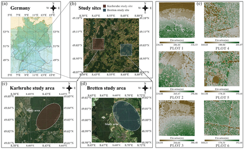
The research area is a mixed forest located in Central Europe, close to Baden-Württemberg in southwestern Germany, with two distinct locations depicted in Figure 1(a–d): Karlsruhe (49°02′ 05.63′′N, 8° 25′ 34.03′′E) and Bretten (49° 00′ 49.64′′N, 8° 41′ 41.39′′E). Both regions experience a temperate maritime climate, with an annual precipitation range of 41-63 mm and a growing season of up to seven months. Both sites have favorable conditions for plant growth, with the average elevation of the Karlsruhe area being approximately 160 m, and Bretten area around 236 m. The former area possesses a gentle terrain with mostly flat land and an average slope of nearly 0°. The latter has a more undulating terrain with an average slope of about 11°, mainly comprising of gentle slopes. The mean values for leaf area index (LAI) and canopy gap fraction (GP) for the two sites are 4.18 and 4.10, and 0.15 and 0.16, respectively. The sites have a diverse range of tree species, including broad-leaved trees like Fagus sylvatica, Acer pseudoplatanus and Carpinus betulus, and coniferous trees like Picea abies, Pseudotsuga menziesii, and Pinus sylvestris. The dominant tree species in the forest, located in the northeastern mountains, are easily identifiable due to numerous intraspecies samples and clear interspecific boundaries. Thus, this area was selected as the primary source of experimental data.

Figure 1. Overview of the research area. (a)–(d) the specific location of the research area; (e) DSM of experimental plots.

2.2. Datasets

The experimental data for two sites were obtained using the RIEGL VQ-780i airborne LiDAR on a Cessna C207 aircraft. Table 1 displays the RIEGL VQ-780i instrument parameters. While collecting data, the aircraft maintained a speed of 5 m/s at an absolute flight height of 650 m. The flight strips were spaced at 175 m. The radar scanned at a pulse repetition rate of 1000 KHz, a frequency of 225 lines/s, a bandwidth of 750 m, and a ± 30° angle. After the scanning process, the original point cloud was initially converted from airborne scanning data using RiANALYZE. GAPOS-corrected data was utilized to estimate flight trajectory data (http://www.sabos.de). Synchronisation of GPS time stamps and specification of geographic coordinates (ETRS 89) followed for merging trajectory and point cloud data. Point cloud data was then converted into the Cartesian UTM coordinate system point cloud (Weiser et al. 2022). The resulting point cloud density for the research area reached 139 pts/m².

Table 1. RIEGL VQ-780i radar equipment parameter information.

Parameters	Specification
Accuracy	20 mm at 250 m scanning range
Precision	20 mm at 250 m scanning range
Laser beam divergence	≤0.25 mrad, full width measured at the 1/e^2 points
Scan angle range	±30°= 60°
Pulse frequency	250000Hz ~ 1000000Hz

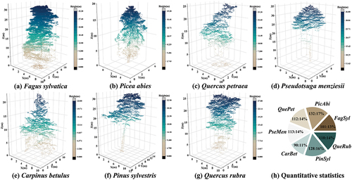
To ensure efficient processing with the algorithm, we partitioned the point cloud data into six experimental plots of equal area, each covering approximately 1 hectare. These plots were identified as PLOT 1 to PLOT 6, of which PLOTs 1 to 3 were from Bretten, and PLOTs 4 to 6 were from Karlsruhe. The general information is displayed in DSM in Figure 1(e), indicating non-uniform distribution of canopy density and surface fluctuation across the six plots. Among all the plots, the dominant tree species with the highest proportion are Fagus sylvatica (FagSyl), Picea abies (PicAbi), Quercus petraea (QuePet), Pseudotsuga menziesii (PseMen), Carpinus betulus (CarBet), Pinus sylvestris (PinSyl) and Quercus rubra (QueRub) (Figure 2). The seven tree species were used in our experiment for classification.

Figure 2. Seven kinds of tree species used in the experiment. (a) Fagus sylvatica; (b) Picea abies; (c) Quercus petraea; (d) Pseudotsuga menziesii; (e) Carpinus betulus; (f) Pinus sylvestris; (g) Quercus rubra; (h) quantitative statistics of all species (number of experimental samples : proportion).

2.3. Experimental sample set construction

In this study, Cloud Compare (CC, https://github.com/CloudCompare), an open source 3D point cloud editing and processing software, was used to edit and process individual tree samples. High-precision ground points were obtained using the Improved Progressive TIN Densification (IPTD) algorithm, with a maximum iteration angle of 10°, a maximum iteration distance of 1.2 m, and a shortest side length of the triangle limited to 1.5 m (Zhao et al. 2016). Next, the Digital Elevation Model (DEM) was generated using Kriging interpolation. The non-ground point cloud, in its rasterized form, was normalized by subtracting DEM to remove any disturbances arising from ground variations.

After ground filtration and elevation normalization was conducted, the individual trees were extracted manually using an interactive segmentation tool in CC. Subsequently, the segmentation findings underwent filtration to remove samples experiencing severe occlusion or adhesion from the canopy point cloud. Figure 2(h) displays the number of trees of each species. Ultimately, we selected 786 high-quality experimental samples, all in a leaf-on state.

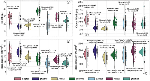
Simultaneously, the height, crown width, mean density, and mean backscattering intensity of the seven tree species were recorded and visualized in Figure 3. As demonstrated in Figures 3(a,b), both Picea abies and Quercus petraea appear to be comparatively smaller than the other species in terms of height and crown width. This observation implies that these two species are relatively undersized. Meanwhile, the height and crown width of the other five tree species are similar (except for the relatively high height of Pseudotsuga menziesii). Furthermore, Figures 3(c,d) demonstrate that the mean density and mean intensity of the seven tree species are comparable (except for the relatively high mean density of Quercus petraea). Therefore, accurately classifying at a global level using geometric domain and intensity domain features may be challenging.

Figure 3. Distribution rain-cloud diagram and statistical details of four characteristics for seven species in the experimental areas. (a) Tree height distribution of the seven species. (b) Crown width distribution of the seven species. (c) Mean density distribution of the seven species. (d) Mean backscattering intensity distribution of the seven species.

Of the 786 trees investigated, 60% were employed to construct training data sets and 40% to construct test data sets. Please refer to Table 2 for the particular number of tree species used in both sets.

Table 2. Specific number of tree species in the training and test sets.

Species	Train	Test	Total
FagSyl	60	41	101
PicAbi	79	53	132
QuePet	67	45	112
PseMen	67	46	113
CarBet	54	36	90
PinSyl	76	52	128
QueRub	66	44	110
Total	469	317	786

3. Methods

3.1. Constructing network input data

3.1.1. Constructing histogram descriptors

Laser point clouds provide valuable information on the distribution of leaves, the structure of branches and the overall shape of different canopies. As a typical geometric feature grounded in the specific tree species, they prove useful in identifying canopies when trees are classified, which has been expressed in previous studies (Axelsson, Lindberg, and Olsson 2018; Holmgren and Persson 2004; Quan et al. 2023). To describe leaf distribution, branch structure, and canopy shape, Lalonde features were extracted from the canopy point cloud, as presented in Figure 4 (Lalonde et al. 2006; Li, Hu, and Noland 2013; Petty et al. 2022). Initially, a spherical neighborhood space was constructed for each point using a particular radius. Then, the dimension features of each point were evaluated by using the eigenvalues λ₁, λ₂ and λ₃ of the covariance matrix composed of the neighborhood point sets, as displayed in Expression (1). DA₁, DA₂ and DA₃ measure the degree of local compliance with point, linear and spherical structures, respectively, while Lalonde features can be obtained through constructing histogram feature descriptors for each. The descriptors of DA₁ and DA₂ indirectly describe leaf distribution and dendritic structure in the canopy, highlighting their overall distribution features. The DA₃ descriptor indirectly gauges the roundness of the canopy through the overall distribution characteristics of its spherical structure. It can subsequently function as a reference point for comparing the shape of canopy.

(1) $D{A}_1=\frac{{\lambda }_1}{\sum _{i=1}^3{\lambda }_i},D{A}_2=\frac{{\lambda }_1-{\lambda }_2}{{\lambda }_1},D{A}_3=\frac{{\lambda }_3}{{\lambda }_1}$(1)

Figure 4. Calculation of five features for a single point using a spherical neighborhood space based on neighboring points.

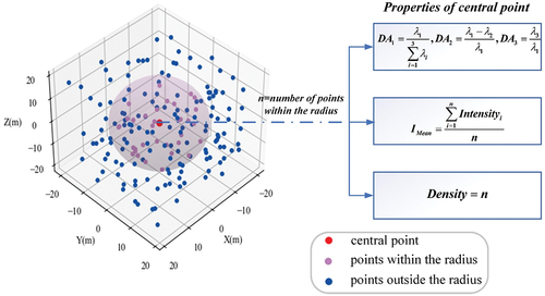
As the quality of feature descriptors is influenced by the neighborhood, whereby minimizing the entropy function, as explained in Expression (2), it can be used to obtain the optimal search radius, R_best, and maintain low uncertainty of DA₁, DA₂ and DA₃ (Xu et al. 2021). According to the definition of entropy, the information contained in the local area of the point cloud can be expressed by information entropy. The smaller the entropy value, the less information the neighborhood contains, that is, the point is less uncertain to obey a certain dimensional feature.

(2) $\left(D{A}_1,D{A}_2,D{A}_3\right)=F\left(R_{best}\right),s.t.min\left(-\sum _{i=1}^{3}D{A}_i{log}^{D{A}_i}\right)$(2)

Differences in leaf size, direction, and density result in varying density and distribution of the canopy point cloud across different tree species (Axelsson, Lindberg, and Olsson 2018; You et al. 2020). Additionally, different types of leaves have different features of intensity, and the distribution difference of canopy density shall also lead to distribution difference of intensity (Korpela et al. 2010; Shi et al. 2018). Consequently, canopy density and intensity characteristics are significant factors in the classification of tree species. Furthermore, numerous studies indicate that the combination of geometrical and intensity features of individual tree point clouds is generally complementary in various details in the classification of tree species. When using such a combination, higher classification accuracy can be achieved in comparison to the use of either feature alone (Axelsson, Lindberg, and Olsson 2018; You et al. 2020; Yu et al. 2017). The current study uses the total number and mean intensity of adjacent points in the spherical neighborhood of each point to reflect local density and intensity levels. Histogram feature descriptors are designed to mirror the distribution features of entire density and intensity. Along with the prior Lalonde functions, five features are derived from each of the singular tree samples.

3.1.2. Refining features

In field applications, the canopy structure, and physical properties of interspecific samples can be highly heterogeneous due to environmental factors such as topography (Qin et al. 2022; Shi et al. 2018; Yu et al. 2017). Directly using individual trees as a feature extraction unit when extracting classification features from the laser point cloud can lead to class imbalance, commonly referred to as the long tail problem. Due to the poor classification results obtained from the data, the most intuitive solution is to address the unbalanced data itself (Megahed et al. 2021). As a result, Lalonde feature, density, and intensity features are not extracted directly from the entire tree. Instead, the tree is evenly divided into slices, and the same feature extraction operation is applied to each slice. As depicted in Figure 5, every slice generates five histogram feature descriptors. Moreover, the statistical intervals of identical features within every slice are uniform, representing the highest and lowest values of the same feature in the whole individual tree sample. This method not only provides a more detailed description of the various features of individual tree samples but also reflects the extracted features’ variation characteristics at the vertical level. In addition, assigning appropriate weights to each component can effectively reduce the feature variance among samples within a species and increase the feature variance among samples from different species. This approach can effectively address classification imbalances.

Figure 5. The single point cloud sample is evenly sliced. The DA₁, DA₂, DA₃, Density, and I_mean of each slice are sequentially calculated, resulting in five histogram descriptors representing the features of each layer.

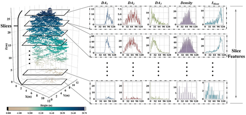
In the experiment, each individual sample tree has 20 slices, and each feature is divided into 128 intervals, which serve as the statistical interval of the histogram. Twenty histogram descriptors of each feature are merged at the one-dimensional level to obtain five 2560-dimensional feature vectors. The five feature vectors are concatenated in sequence to obtain a 12,800-dimensional feature vector, which describes the characteristics of each tree sample and serves as the classification network’s input vector. Nevertheless, the substantial dimension of input vectors not only results in the algorithm’s increased time and space complexity, but also enhances the network’s susceptibility to overfitting due to the non-uniform distribution of data sparsity in the search area. To prevent overfitting, reduce computational complexity, and improve the network’s generalization ability, it is imperative to reduce the dimensionality of the data before training commences, as illustrated in Figure 6(a). Let there be n∈N samples, each composed of m∈N slices, and let the histogram of each feature separate i∈N statistical intervals. All feature histograms are transformed at the two-dimensional level, with each sample consisting of a feature vector size of (5 × m, 1, i). Principal Component Analysis (PCA) is then applied to map the 5×m feature vector of each layer from i dimension to j dimension linear subspace. This reduces the vector dimension and enhances the feature variance of interspecific samples. Following this, each feature vector is flattened to obtain the feature vector that are ultimately inputted into the network. In the experiment, where i = 128, the PCA projection error (PE) is calculated, as stated in Expression (3):

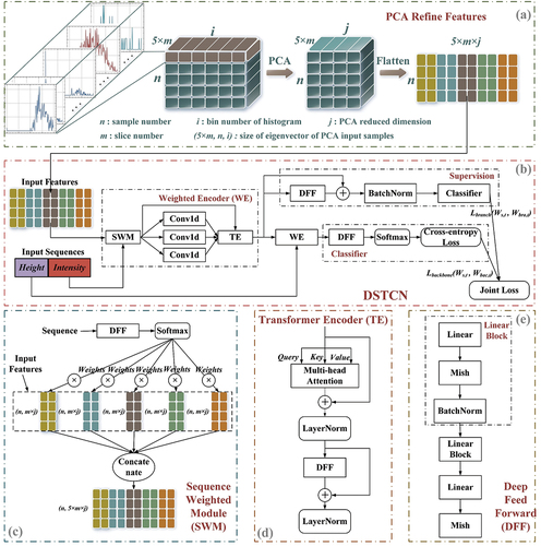
Figure 6. The architecture of DSTCN is shown in detail in the figure. (a) Constructing input vector based on PCA. Histogram feature descriptors of individual tree samples stitched at the two-dimensional level and subjected to low-dimensional mapping and linear reconstruction using PCA. The resulting dimensionality-reduced feature vectors are fed into the deeply supervised network DSTCN for tree species classification; (b) DSTCN architecture; (c) sequence weighted module structure; (d) transformer encoder structure; (e) deep feed forward structure.

(3) $PE=1-\frac{\sum _{k=1}^j{S}_k}{\sum _{k=1}^i{S}_k}$(3)

where S is the matrix of eigenvalues obtained through Singular Value Decomposition (SVD) of the covariance matrix in PCA. When the value of PE approaches 0.01, the dimension is reduced to 66 after dimensionality reduction, and we have chosen j = 64 such that the information remains close to 99% even after dimensionality reduction. The final dimension of the input vector is 6400.

3.2. Tree species classification network

With regards to the feature vectors that were extracted, this study has devised a deep supervision network DSTCN that employs height-intensity dual attention mechanisms. The exact configuration of the network is illustrated in Figure 6. The network receives the originally extracted feature vectors as its input and generates end-to-end classification outcomes. The main components of the network architecture are the Weighted Encoder (WE), comprising the Sequence Weighted Module (SWM) and Transformer Encoder (TE), and the Deep Feed Forward (DFF) structure. The two WEs work in tandem to increase attention height and intensity, assigning multiscale attention to features by combining SWM and TE. Additionally, an auxiliary branch model is added after the first WE to form the Intermediate Supervision (IS) for the backbone network. A more detailed explanation of the network architecture design will follow.

3.2.1. Height-intensity attention feature weighting

The study indicates that the intensity features of an individual tree point cloud obtained during the leaf-on state can serve as a crucial characteristic to describe canopy index. Furthermore, the LiDAR index for tree species classification that holds the most power is the mean intensity or mean echo width of the initial or sole echo (Chamberlain, Meador, and Thode 2021; Shi et al. 2018). Due to environmental variation between regions, differences in the canopy density of intraspecific samples can occur. In middle and low canopies, varying degrees of shading can cause significant differences in the point cloud density and geometric morphology of intraspecific samples, ultimately influencing the accuracy of classification. With airborne LiDAR’s top-down scanning characteristics, slices nearer the top of the same canopy usually have greater acquisition points of the first echo, as well as higher mean intensity and mean density. For individual tree sample sets where height is normalized, more focus ought to be given to slices featuring higher levels of mean height and mean intensity, as they aid in elucidating the biological differences between tree species. As such, the network is designed with SWM, and Figure 7 shows the specific structure. Extract the mean intensity and mean height of each slice in every individual tree sample, and create an intensity sequence $\text{if}intensity=\left\{i_s^1,i_s^2,i_s^3,...,i_s^m\right\}m\in N$ and height sequence $\text{if}Height=\left\{h_s^1,h_s^2,h_s^3,...,h_s^m\right\}m\in N$ for each tree sample. The slice information sequence constructed is analyzed by DFF in SWM and Softmax generates the normalized slice weight. Next, the features in various slices are assigned weights. By following this approach, the network concentrates its attention on slices exhibiting greater heights and intensities.

Figure 7. Generation of normalized weights by sequence weighted module (SWM) based on height or intensity sequences, using DFF plus softmax. The SWM assigns features belonging to different slicing layers in the original input vectors.

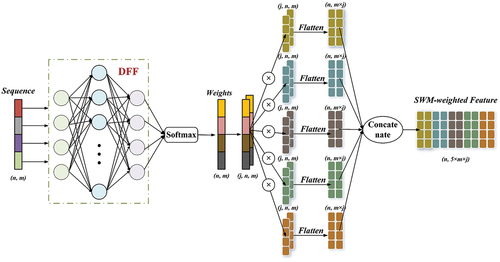
The allocation of attention to the feature scale is enhanced through a TE in addition to the weight generation by the height/intensity sequence in the SWM. Initially, three one-dimensional convolutional layers generate transformation matrices (Query, Key, Value) for the input features through distinct linear mappings. The TE receives the SWM-weighted feature vector in addition to the Query, Key and Value, as illustrated in Figure 8. The MHA mechanism generates the feature correlation weight matrix by applying the Query and Key and then combines the Value for obtaining final weighted output. Following this, residual connection is implemented with the SWM-weighted feature vector. LayerNorm is then used to normalize the feature dimension (Takagi, Yoshida, and Okada 2019). Ultimately, to improve the features’ performance, deep coding is executed using the DFF.

Figure 8. Allocation of attention to features at the slice level by Sequence Weighted Module (SWM), followed by allocation of attention at the feature level by multi-head attention (MHA) of transformer encoder (TE). The SWM-weighted feature and MHA-weighted feature are then inputted into the deep feed forward (DFF) through residual linkage, enhancing the feature’s expressive capability.

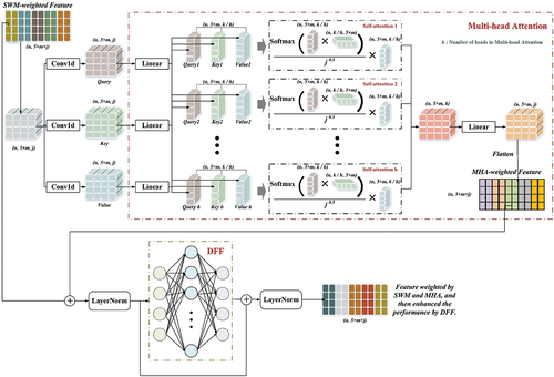
These improvements facilitate a more intricate allocation of attention at the feature scale, considering the intricacy of the individual slices with five features and 128 statistical intervals each. Through incorporating TE, the model heightens the feature interactions and captures their dependencies competently. Consequently, the classification results’ precision and performance are further improved. Through these modifications, the proposed method combines SWM weighting with TE to achieve a more precise and comprehensive allocation of attention at both slice and feature scales. Thus, available information is effectively utilized, enhancing the overall performance of the classification network.

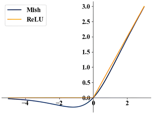
The DFF structure involved in SWM and TE is depicted in Figure 7d. It comprises of a consecutive sequence of three linear mapping layers. The activation function implemented in DFF is Mish, as illustrated in Expression (4) (Mondal and Shrivastava 2022). The input variable used by the activation function multiplies its activation value after accomplishing a nonlinear change, which possesses boundless characteristics and is more fault tolerant in the negative region, as demonstrated in Figure 9. Compared to the frequently employed ReLU (Rectified Linear Unit), Mish successfully resolves the saturation issue caused by ReLU’s rigid zero boundary, avoids gradient disappearance, and achieves enhanced and smoother gradient flow, benefiting the network to attain better precision and generalization.

Figure 9. A comparison of the activation functions Mish and ReLU. Mish exhibits better inclusiveness in the negative region and appears smoother in comparison to ReLU.

(4) $Mish:f\left(x\right)=x\times tanh\left(l{n}^{1+e^x}\right)$(4)

3.2.2. Intermediate supervision

Although the Mish activation function is utilized within the network boundary, the backpropagation process may cause the gradient to vanish or explode due to the multidimensional nature of the training data. This phenomenon can lead to slow convergence, non-convergence, or convergence to a local optimal solution (Shi et al. 2020). However, incorporating intermediate supervision within the network can be an effectively solution. Intermediate supervision adds a direct layer of supervision for the hidden layer by including an adjoint loss function to the hidden layer. The supervision results are then sent straight back to the previous layer, enhancing the gradient flow in the network and increasing its stability (Luo, Li, and Shen 2020; Sheng et al. 2022). For a lightweight network like DSTCN, intermediate supervision can enhance the discrimination and robustness of the learning features of the hidden layer, as powerful regularization, and reduce the distribution deviation of related variables within the network. This approach effectively improves the representation ability and increases the convergence speed of the network to some extent.

In the DSTCN backbone, the network model is built by linking Softmax via DFF, with cross-entropy loss serving as the targeted loss function. Nevertheless, in the supervised segment, if the model is hooked up directly to the superficial hidden layer, it compels the shallow hidden layer to extract profound features beyond its jurisdiction (Sun et al. 2019). Therefore, a DFF is included in the supervised branch to extract depth features and the model is sequentially connected to ensure step-by-step feature extraction. The added DFF employs a residual connection to maintain gradient stability. This section of the model trains the weighted characteristics of the intensity sequence and computes the branch classification loss L_branch(W_s,t, W_bra,t) in the shallow hidden layer. The gradient is then propagated back to the early layer and enhances its training. The overall loss of the network consists of the branch classification loss L_branch(W_s,t, W_bra,t) and backbone classification loss L_backbone(W_s,t, W_bac,t). W_s,t represents the hidden layer parameters shared by the branch and backbone, whereas W_bac,t and W_bra,t represent the parameters of the distinct parts of the backbone and branch respectively. An expression (5) shows the joint loss function of the branch and the backbone loss.

(5) $L\left(W_{s,t},W_{bac,t},W_{bra,t}\right)=L_{backbone}\left(W_{s,t},W_{bac,t}\right)+w_{bra,t}{L}_{branch}\left(W_{s,t},W_{bra,t}\right)$(5)

The weight coefficient w_{bra, t} of branch loss is dynamically adjusted by HydaLearn (Highly Dynamic Learning), which is a weight adjustment method based on the correlation of the gain values of backbone and branch loss after gradient updating (Verboven et al. 2022). In t^th forward propagation, the increase in the backbone loss value γ_bac,t and the increase in the branch loss value γ_bra,t can be determined by calculating the difference between the loss values prior to and following the gradient update illustrated in Expression (6). The proportion of the backbone loss weight coefficient w_bac,t to the branch loss weight coefficient w_bra,t can be approximated as the ratio of loss gain. After determining the gain-loss ratio, the weight coefficient w_bac,t for the backbone loss is assigned a value of 1. Subsequently, the weight coefficient w_bra,t for the branch loss is calculated as the inverse of the gain-loss ratio.

(6) $\frac{w_{bac,t}}{w_{bra,t}}\approx \frac{{\gamma }_{bac,t}}{{\gamma }_{bra,t}}=\frac{L_{backbone}\left(W_{s,t},W_{bac,t}\right)-L_{backbone}\left(W_{s,t-1},W_{bac,t-1}\right)}{L_{branch}\left(W_{s,t},W_{bra,t}\right)-L_{branch}\left(W_{s,t-1},W_{bra,t-1}\right)}$(6)

3.3. Benchmark methods and training parameters

DSTCN was compared to two frequently used classification algorithms for point cloud tree species. The first algorithm classified point cloud directly based on Point Net++ (Liu et al. 2022). The second algorithm extracted individual features of the tree parameters through feature engineering and subsequently employed BP Net (Back Propagation Net) for classification (Lin and Hyyppä 2016; Michałowska and Rapiński 2021). Farthest Point Sampling (FPS), K-means Sampling (KS), Random Sampling (RS), Grid Average Sampling (GAS), and Non-uniform Grid Sampling (NGS) were employed in Point Net++. The experimental data underwent Multi-scale Grouping (MSG) sampling. To adhere to limitations of the experimental sample point cloud, the number of single sample samples was set to 1024, 2048, and 3072, respectively.

Geometric features (GE) and single-channel intensity features (CI) were extracted in the BP Net classification method, as indicated in Tables 3 and 4. During the experiment, tree species were categorized based on geometric features and geometric-intensity joint features. BP Net adopts the design of two hidden layers, and uses Genetic Algorithm (GA) to adjust the parameters adaptively.

Table 3. Geometry parameters (GE) of individual trees.

Features	Definition
Hmax	Maximum value of point cloud normalized height
Hmean	Arithmetic mean of point cloud normalized height
Hstd	Standard deviation of point cloud normalized height
Hmed	Median of point cloud normalized height
Hrange	Range of point cloud normalized height
HP10–90	The ratio of the sum of height values of point cloud with heights higher than n%Hrange to the sum of height values of the overall point cloud (n∈[10, 90])
PR	Ratio of the number of returns from points below a specified height to the total number of returns, also known as penetration rate
Carea	Surface area of crown convex package
Cvol	Volume of crown convex package
Cdia	Diameter of the fitted circle of the vertical projection of the canopy
Casy	Difference in crown length between two orthogonal directions in the vertical projection of the canopy
Cden	Crown density
D1–10	Divide Hrange equally into ten height layers and calculate the ratio of the number of point cloud within each layer to the total number of point cloud in an individual tree

Table 4. Single channel intensity parameters (CI) of individual trees.

Features	Definition
Imax	Maximum value of point cloud intensity
Imin	Minimum value of point cloud intensity
Imean	Arithmetic mean of point cloud intensity
Imed	Median of point cloud intensity
Istd	Standard deviation of point cloud intensity
Ivar	Coefficient of variation of point cloud intensity
Isk	Skewness of point cloud intensity
Iku	Kurtosis of point cloud intensity
Irange	Range of point cloud intensity
I10–90	The ratio of the sum of intensity values of point cloud with intensity greater than n%Irange to the sum of intensity values of the overall point cloud (n∈[10, 90])

All experiments were carried out on a workstation running an lntel(R) Core(TM) i7-9700K CPU (3.60 GHz (8 CPUs)). The chosen programming language was Python 3.8.5, and the deep networks utilized Pytorch 1.13.1. Due to variations in input features, DSTCN and BP Net were trained with a batch size of 64, while Point Net++ used a batch size of 32. During the network’s training process, AdamW and SGD were employed for optimization. The initial 60 Epochs benefited from rapid gradient descent with the AdamW optimizer, while the full training spanned 100 Epochs. The initial learning rate was 1e-3 and the exponential decay rates of the first and second moment estimations were 0.9 and 0.999 respectively, while the regularization was based on the weight decay index of 1e-3. To achieve more appropriate tuning when the gradient was gradually stable, SGD replaced AdamW. The SGD learning rate was 1e-5 and the momentum was 0.7. Gradient descent was accelerated using the Nesterov Accelerated Gradient (NAG) method (Lin et al. 2019; Loshchilov and Hutter 2017).

3.4. Accuracy assessment

The evaluation of classification accuracy for each tree species was done by computing the F1-score in the experiment. The overall classification quality was assessed through the Macro Average Precision (MAP), Macro Average Recall (MAR), Macro Average F1-score (MAF), Overall Accuracy (OA), and Kappa coefficient. MAP, MAR, and MAF are calculated as the arithmetic mean of precision, recall, and F1-score for individual tree species, with each class being treated equally and the number of tree species unconsidered. These metrics can effectively reflect the overall performance of precision, recall, and F1-score in a single classification experiment when the data for various tree species are similar (Li et al. 2022). OA intuitively indicates the classifier’s accuracy by calculating the ratio of positive samples. On the other hand, the Kappa coefficient indicates the ratio of classification results that do not involve any unexpected deviations; it reflects the consistency between the predicted outcomes of the model and the actual classification situation (Michałowska and Rapiński 2021). Meanwhile, we evaluated the dispersion of interspecies classification accuracy in each experiment by calculating the Interspecies Standard Deviation (ISD) values of Precision, Recall, and F1-score, including PISD, RISD, and FISD. The formulas for all accuracy assessment metrics are shown in Table 5.

Table 5. The formulas for all accuracy assessment metrics.

Variable Definition	Metrics	Formulas
TPi (True Positive of species i)	MAP (Macro Average Precision)	$\frac{1}{n}{\sum }_{i=1}^n\frac{T{P}_i}{T{P}_i+F{P}_i}$
TNi (True Negative of species i)	MAR (Macro Average Recall)	$\frac{1}{n}{\sum }_{i=1}^n\frac{T{P}_i}{T{P}_i+F{N}_i}$
FPi (False Positive of species i)	MAF (Macro Average F1-score)	$\frac{1}{n}{\sum }_{i=1}^n\frac{2T{P}_i}{2T{P}_i+F{P}_i+F{N}_i}$
FNi (False Negative of species i)	PISD (Interspecies Standard Deviation of Precision)	$\sqrt{\frac{1}{n}{\sum }_{i=1}^n{\left(\frac{T{P}_i}{T{P}_i+F{P}_i}-\mathrm{M}\mathrm{A}\mathrm{P}\right)}^2}$
RSZi (Real Sample Size of species i)	RISD (Interspecies Standard Deviation of Recall)	$\sqrt{\frac{1}{n}{\sum }_{i=1}^n{\left(\frac{T{P}_i}{T{P}_i+F{N}_i}-\mathrm{M}\mathrm{A}\mathrm{R}\right)}^2}$
PSZi (Predicted Sample Size of species i)	FISD (Interspecies Standard Deviation of F1-score)	$\sqrt{\frac{1}{n}{\sum }_{i=1}^n{\left(\frac{2T{P}_i}{2T{P}_i+F{P}_i+F{N}_i}-\mathrm{M}\mathrm{A}\mathrm{F}\right)}^2}$
	OA (Overall Accuracy)	$\frac{{\sum }_{i=1}^{n}T{P}_i+T{N}_i}{{\sum }_{i=1}^{n}T{P}_i+F{P}_i+T{N}_i+F{N}_i}$
	Kappa	$\frac{\mathrm{O}\mathrm{A}\ast {\left({\sum }_{i=1}^{n}RS{Z}_i\right)}^2-{\sum }_{i=1}^{n}RS{Z}_i\ast PS{Z}_i}{{\left({\sum }_{i=1}^{n}RS{Z}_i\right)}^2-{\sum }_{i=1}^{n}RS{Z}_i\ast PS{Z}_i}$

4. Results

4.1. Classification results analysis

The classification outcomes of DSTCN, Point Net++, and BP Net are presented in Table 6. It demonstrates that the NGS sampling method and 3072 sampling points with Point Net++ produces the highest accuracy in direct point cloud classification. On the other hand, when utilizing the combined features of geometry and intensity, the feature vector classification method based on BP Net has the highest classification accuracy. Compared with other methods, the classification results obtained using DSTCN are noteworthy. Specifically, in the evaluation metric of mean average precision (MAP), DSTCN results were found to be 7–13% higher than those achieved by Point Net++ and 8–11% higher than those by BP Net. Mean average F1-score (MAF) showed a 6–13% improvement with DSTCN compared to Point Net++, and 8–11% improvement compared to BP Net. In terms of mean average recall (MAR), DSTCN performance was 7–14% higher than Point Net++ and 9–12% higher than BP Net. Overall accuracy (OA) was 6–12% higher with DSTCN compared to Point Net++ and 7–11% higher compared to BP Net. The Kappa coefficient is significantly greater than that of Point Net++ by 7–15%, and BP Net by 8–13%. Therefore, DSTCN’s classification accuracy considerably surpasses that of other methods.

Table 6. Classification experiment results for DSTCN, point Net++, and BP net.

Methods	Num of samples	MAP	MAR	MAF	PISD	RISD	FISD	OA	Kappa
Point Net++ (FPS)	1024	0.82	0.81	0.81	0.04	0.06	0.03	0.82	0.78
	2048	0.83	0.82	0.82	0.11	0.06	0.09	0.83	0.80
	3072	0.85	0.84	0.84	0.06	0.08	0.06	0.84	0.82
Point Net++ (KS)	1024	0.82	0.82	0.82	0.04	0.09	0.06	0.82	0.79
	2048	0.87	0.86	0.86	0.06	0.04	0.04	0.86	0.84
	3072	0.87	0.87	0.87	0.07	0.06	0.04	0.87	0.85
Point Net++ (RS)	1024	0.83	0.82	0.82	0.10	0.07	0.06	0.82	0.78
	2048	0.83	0.83	0.83	0.06	0.08	0.06	0.83	0.80
	3072	0.86	0.86	0.85	0.08	0.06	0.05	0.85	0.83
Point Net++ (GAS)	1024	0.83	0.84	0.83	0.08	0.06	0.06	0.83	0.80
	2048	0.85	0.84	0.84	0.10	0.09	0.07	0.85	0.82
	3072	0.86	0.86	0.86	0.07	0.06	0.05	0.86	0.84
Point Net++ (NGS)	1024	0.84	0.83	0.83	0.06	0.13	0.09	0.83	0.80
	2048	0.86	0.85	0.85	0.08	0.07	0.05	0.85	0.83
	3072	0.88	0.88	0.88	0.09	0.08	0.08	0.88	0.86
BP Net (GE)		0.84	0.83	0.83	0.10	0.11	0.08	0.83	0.80
BP Net (GE+CI)		0.87	0.86	0.86	0.10	0.08	0.06	0.87	0.85
DSTCN		0.95	0.95	0.94	0.03	0.03	0.02	0.94	0.93

Meanwhile, Table 6 presents the calculation results of ISD, which indicate that DSTCN has the lowest values for all three indices among all experiments, with no equivalent levels in any other. Possible reasons for this outcome will be analyzed next.

Firstly, the feature engineering of either Point Net++ that directly processes the individual tree point cloud or BP Net that extracts and then classifies the individual tree parameters. This is carried out at the global level for each individual tree. Various factors, including undulating terrain, varying laser scanning angles, and changes in flight altitude during scanning, can heighten the distinct noise of intraspecific samples at differing vertical levels. This can consequently lead to model misinterpretation.

When assessing solely the geometric features globally, misjudgment may occur with species like Fagus sylvatica and Quercus rubra, as they lack clear spatial structure (Figure 2) and notable biological attribute parameters (Figure 3(a,b)), ultimately decreasing the overall classification accuracy (Figure 10(a)). In the mean time, if the intensity distribution of all tree species globally is similar (Figure 3(d)), introducing intensity features at a worldwide level may not significantly aid effective classification, but rather result in a more chaotic feature space (Figure 10(b)). Consequently, although the accuracy of certain species’ classification may be effectively enhanced, the overall classification accuracy will be significantly compromised. However, DSTCN’s feature engineering is based on the individual tree slice level, which provides a more detailed analysis than the global level of an individual tree, considering the possible feature noise at different vertical heights influenced by various factors. Even though the OA of different tree species in DSTCN’s classification results is not bound to be guaranteed to be higher than other methods, its overall OA is not only high but also evenly distributed (Figure 10(c)).

Figure 10. Confusion matrix based on a part of excellent classification results of point Net++, BP net and DSTCN. (a) Point Net++ (NGS, 3072); (b) BP net (GE+CI); (c) DSTCN; (d) F1-score of seven species.

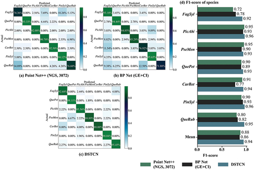
Considering that OA can only reflect the proportion of correct classification of tree species, we draw the F1-score distribution bar chart as shown in Figure 10(d). F1-score comprehensively considers Recall and Precision, so it can reflect the influence of single species on other species from the side. For example, the classification result of Fagus sylvatica in BP Net, although the OA is high, produces more misjudgments in other tree species, so its F1-score is low. Only in the classification results of DSTCN were the OA and F1-score of all types of tree species maintained at a high level. This proves DSTCN’s superior ability to extract deep feature differences in species samples with similar morphology, in contrast to Point Net++ and BP Net classification, which concentrate more on the global features of individual trees. Therefore, all kinds of tree species are not only correctly classified, but also have less interspecific misclassification, which minimizes the influence of interspecific differences and ensures the overall high classification accuracy.

4.2. Robustness and generalization tests

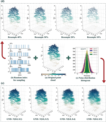
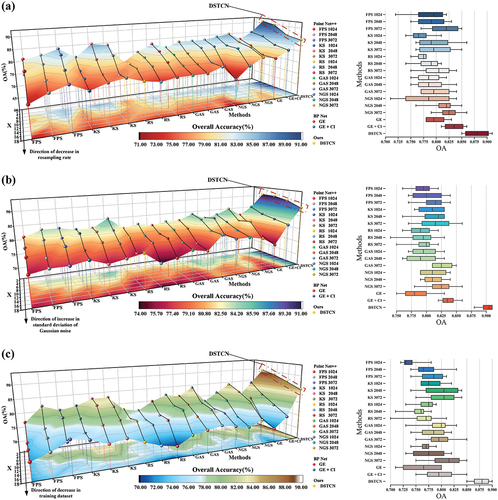
To enhance the assessment of DSTCN’s performance, we conducted robustness experiments that incorporated randomly downsampling and adding Gaussian noise to the point cloud in the spatial domain, a graph of the experimental structure can be seen in Appendix A (Qi, Su, et al. 2017; Qi, Yi, et al. 2017). The random downsampling aimed to simulate the stochastic effects of airborne LiDAR on forest acquisitions of stand details attributable to varying terrain relief, altered flight conditions, and other factors that might occur during data acquisition. Gaussian noise was used to simulate the perturbations that occur during data acquisition by the LiDAR sensor. Additionally, experiments were conducted to test generalization using a smaller training dataset. The sampling rate for random downsampling was gradually reduced from 40% to 10% in 10% increments. The standard deviation of the Gaussian noise was increased from 0.2 to 0.5 in increments of 0.1. As the percentage of the training dataset within the overall dataset decreased gradually from 60% to 30% by steps of 10%, the percentage of the test dataset remained constant at 40%. The outcomes regarding overall accuracy for all three experiments are illustrated in Figure 11. The 3D line graph and box plots illustrate DSTCN’s consistent attainment of the highest overall accuracy despite varied experimental conditions. To obtain a two-dimensional representation, we utilized OA to generate a surface which was then projected onto a horizontal plane. By mapping the color to horizontal projection, our results show that DSTCN is always superior to other methods, and it has the maximum representation of high OA areas, while maintaining a high homogeneity (Michałowska and Rapiński 2021). The findings from the robustness experiments indicate that DSTCN possesses outstanding adaptability and processing proficiency for residual or noisy data. DSTCN differs from other classifiers by its capacity to efficiently capture and acquire meaningful features from chaotic and disturbed backgrounds. This leads to more precise classification outcomes. The classifier’s robustness enables it to handle noisy data and uncertain environments with great dexterity and makes it particularly suitable for such settings. Meanwhile, the findings of the generalization experiments conducted with varying training volumes demonstrate that DSTCN can rapidly learn efficient classification characteristics even with limited data, and can perform data feature analysis and generalization. These outcomes reiterate the conclusion drawn from the confusion matrix illustrated in Figure 10, that DSTCN can effectively suppress feature noise and enhance robustness for intraspecies samples. Compared to other classification methods in the control experiments, DSTCN can effectively extract depth feature discrepancies between samples.

Figure 11. Results of robustness experiments and generalization experiments. (a) Results of random downsampling experiments; (b) results of Gaussian noise perturbation experiments; (c) results of decreasing experiments on the training dataset.

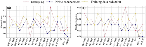
Meanwhile, we computed the absolute range and standard deviation of OA for every classifier under varying conditions and graphed them on a line chart, illustrated in Figure 12. It can be observed that BP Net (GE+CI) and DSTCN have a near-equal absolute range and standard deviation, and are generally superior to most other methods in terms of robustness experiments, notwithstanding a significant OA level discrepancy. We posit that this occurs due to the use of intensity information in both methods. Downsampling and noise both target the spatial domain features of the point cloud, thus heavily impacting the spatial geometry of the samples, whereas the intensity features remain relatively stable. Furthermore, both methods can take in input vectors obtained through statistical feature engineering, which results in superior stability and accuracy when faced with perturbed data. Using only spatial features can make other methods somewhat challenging. Therefore, it can also be shown that statistical histogram-based feature engineering is related to the utilization of intensity information to keep the robustness of DSTCN high.

Figure 12. Absolute range and standard deviation of OA obtained by various methods under different experiments.

4.3. Ablation study

To more accurately assess the impact of implementing height-based WE (HWE) and intensity-based WE (IWE) in DSTCN on classification efficiency, we conducted an ablation study. The study involved testing various combinations (VN, VN+HWE, VN+IWE, VN+HWE+IWE) of HWE, IWE, and Vanilla Net (VN) for classification experiments without IS. Additionally, we added IS to each experimental group to investigate its specific role in the design. The construction sequence of various network combinations and their respective experimental outcomes are presented in Table 7.

Table 7. Network construction sequence of different combinations and the corresponding ablation study results.

Models	MAP	MAR	MAF	PISD	RISD	FISD	OA	Kappa
VN (DFF+Classifier)	0.85	0.84	0.84	0.06	0.09	0.04	0.84	0.82
VN+HWE (HWE+Classifier)	0.86	0.87	0.86	0.09	0.06	0.04	0.86	0.84
VN+IWE (IWE+Classifier)	0.89	0.89	0.89	0.03	0.06	0.03	0.89	0.87
VN+HWE+IWE (HWE+IWE+Classifier)	0.93	0.93	0.93	0.03	0.04	0.02	0.93	0.92
VN+IS (DFF+IS+Classifier)	0.84	0.85	0.84	0.06	0.09	0.04	0.85	0.83
VN+HWE+IS (HWE+IS+Classifier)	0.86	0.87	0.86	0.08	0.06	0.04	0.86	0.84
VN+IWE+IS (IWE+IS+Classifier)	0.89	0.89	0.89	0.03	0.06	0.03	0.89	0.87
VN+HWE+IWE+IS (HWE+IS+IWE+Classifier)	0.95	0.95	0.94	0.03	0.03	0.02	0.94	0.93

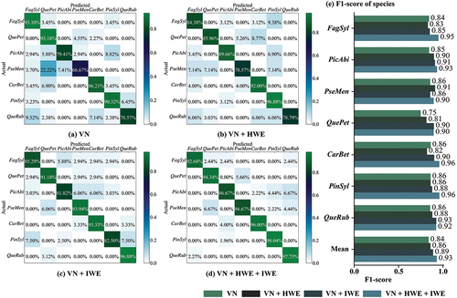
Based on the findings presented in Table 7, it is apparent that the combination of VN+IWE yielded more favorable classification outcomes when compared to the VN+HWE combination. Therefore, we can draw a conclusion that intensity information is a more important than the height information when highlighting the differences among tree species. Although combining VN+HWE+IWE leads to better results than using only VN+HWE/IWE, the study highlights the significance of using intensity and height information in conjunction for distinguishing between different tree species’ features. To further investigate the classification outcomes for various combinations, we plotted the confusion matrix and F1-score bar chart depicted in Figure 13, demonstrating the changes of classification at the tree species level. The color distribution depicted in Figure 13(a–d) shows that HWE and IWE technologies can effectively alleviate the high misjudgment, as proved by the concrete examples of Pseudotsuga menziesii and Quercus rubra. The evident comparison between VN+IWE and VN+HWE shows that the former is more effective, and the combination of the two produces the most remarkable results. This can be clearly discerned from the data depicted in Figure 13(e). In the F1-score for various tree species, VN+IWE mostly yields higher results than that of VN+HWE. Additionally, the combination of both leads to the highest accuracy. These findings support the hypothesis that distributing attention information across different levels generates more well-proportioned classification outcomes.

Figure 13. Confusion matrix based on classification result of adding HWE and IWE respectively. (a) VN; (b) VN + HWE; (c) VN + IWE; (d) VN + HWE + IWE; (e) F1-score of seven species.

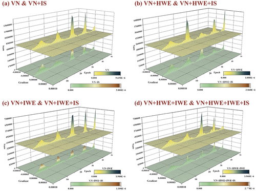
When the inclusion of IS is implemented, the classification accuracy of each combination does not demonstrate a significant improvement, as evidenced by Table 7. Figure 14 displays the gradient histogram flow changes from our calculation. Each graph illustrates the variation in gradient flow between the input layer and the DFF during training, both with and without IS, for the same early hidden layer. When Instance Normalisation (IS) is added, it significantly moderates the gradient flow of the hidden layer and reduces the likelihood of excessive kurtosis. Therefore, it has been proven that although IS does not have a significant impact on improving classification accuracy, it can effectively moderate the gradient flow of the early hidden layer, thus avoiding issues such as gradient disappearance or gradient explosion of the network during the training process.

Figure 14. The difference between the gradient change in training is shown by counting the same early hidden layer with or without IS. (a) Comparison between VN and VN+IS; (b) comparison between VN+HWE and VN+HWE+IS; (c) comparison between VN+IWE and VN+IWE+IS; (d) comparison between VN+HWE+IWE and VN+HWE+IWE+IS.

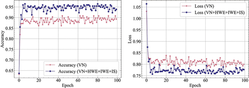
Meanwhile, the training progress of VN and VN+HWE+IWE+IS was graphed and displayed in Figure 15. It was observed from the graph that the latter demonstrated both a notably quicker convergence rate and higher accuracy, whilst also displaying less loss compared to the former. These results confirm the efficacy of the designed module.

Figure 15. Comparison of accuracy and loss during training of VN and VN+HWE+IWE+IS.

5. Discussion

5.1. Feature vector quality impact factors

When feature vectors are extracted from individual tree samples, the quality and dimension are affected by three factors.

1. Number of individual tree’s sliced layers (NSL).

2. Number of statistical intervals in the construction of histogram feature descriptors (NSI).

3. PCA spatial compression degree (PSCD). It is the ratio of the difference between the dimension of PCA mapping subspace and the dimension of original space to the dimension of original space.

In order to accurately understand the importance of the above factors in the process of feature vector extraction, we have conducted many experiments with different combinations of factors and used OA to measure the accuracy. The values for the three factors can be found in Table 8. After multiple instances of experimentation, the statistical results displayed in Figure 16 were obtained, PSCD decreases in order from a to d. Observing the given information, we can deduce that under each PSCD, when NSL is kept constant, OA tends to decrease with decreasing NSI. Due to a high number of NSI, the feature distribution is elaborated in detail. In theory, higher NSI provides adequate enough information to make it directly proportional to OA. However, if NSI is kept constant, NSL changes do not seem to have a significant impact on OA. This may be because DSTCN’s SWM dynamically assigns weights to each slice. Under this adaptive mechanism, the relevance between NSL and final OA is significantly decreased, which leads to no notable alteration in graphics.

Figure 16. The OA obtained after repeated experiments with changed NSL, NSI and PSCD in the feature engineering multiple times. (a) OA of different NSL and NSI under 50% PSCD; (b) OA of different NSL and NSI under 40% PSCD; (c) OA of different NSL and NSI under 30% PSCD; (d) OA of different NSL and NSI under 20% PSCD.

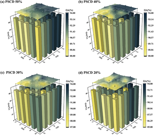
Table 8. Repeat the test experiment for the specific values of the three possible influencing factors.

Number of sliced layers	Number of statistical intervals	PCA spatial compression degree
20	128	50% 40% 30% 20%
18	112
16	96
14	80
12	64

Overall, as PSCD decreases, the distribution of OA becomes more chaotic. The sum of variances increases as the number of PCA dimensions decreases and the PSCD decreases, indicating that more information is preserved. However, because PCA is unsupervised, it follows the hypothesis principle when classification labels are constrained: the signal-to-noise ratio is higher with larger variances. There could be some invalid features in the original data that are not useful for classification. Using an excessive PSCD can lead to the retention of invalid features and an increase in their variance, resulting in more data noise. This may be why lower PSCDs in Figure 16 produced a more ambiguous overall OA distribution. Additionally, it is not accurate to assume that higher PSCDs lead to higher OA, as evident in the OA of NSL and NSI fixed under differing PSCDs. In practical applications, the exact condition where features become invalid remains unclear, and the appropriate PSCD also has a connection to NSI, necessitating multiple manual adjustments.

5.2. Applicability and limitations

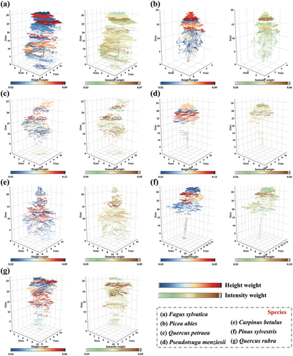
The effectiveness of the proposed method can be evaluated from two aspects. Firstly, in the ablation study, it has been demonstrated that both HWE and IWE contribute to improving and balancing the accuracy. We assign colors to the vertical parts of the samples based on the Softmax outputs of HWE and IWE, as displayed in Figure 17. The height and intensity information structure focuses on the upper canopy with higher density and richer features while disregarding the lower canopy that lacks features. This effectively prevents the lower canopy features from excessively interfering with classification. This also corroborates the findings outlined in Table 7, indicating the network classification accuracy is progressively enhanced with the implementation of HWE and IWE (F1-score, OA, Kappa, etc. increase steadily), and the classification precision of different tree species is more consistent (FISD gradually decreases). In practical application scenarios, this design avoids the direct comparison of characteristics between different monomers at the global level, thus avoiding misjudgment caused by sample differences (biological structure differences, point density differences, reflection intensity differences, etc.) between the same kind of samples due to different tree ages (differences in biological attribute parameters such as tree height and crown width) or different scanning conditions and environments (differences in scanning angle, scanning height, shielding degree, etc.).

Figure 17. Colorized sample slices of different tree species based on the weights of softmax outputs in height weighted encoding (HWE) and intensity weighted encoding (IWE). This clearly reflects the attentional distributions of height information and intensity information constructs.

Secondly, the analysis of DSTCN architecture (Figure 6) shows it is mostly composed of linear layers. Therefore, compared with Point Net++ whose depth and width are equivalent, although the number of Parameters in the linear layer is obviously higher than that in the convolution layer (parameters, DSTCN: 61.23 M, Point Net++: 1.74 M), the matrix-based operation mode of the linear layer has a clear advantage in operation speed over the convolution layer based on sliding window dot product, which can be seen from the Floating Point Operations (FLOPs) (FLOPs, DSTCN: 0.41 G, Point Net++: 13.29 G). In the training process, despite the differences in Batch Size, DSTCN needs only 6s on average, while Point Net++ needs 300s on average. With speed and accuracy advantages, DSTCN delivers higher treatment efficiency, and therefore is more suitable for the practical application of large-scale tree species classification in multi-layer mixed forest.

However, this proposed method has its limitations. Firstly, the features extracted from the feature engineering method are histogram descriptors, which cannot directly provide the biological or physical information of individual trees, and therefore it cannot be directly applied to the expansion of individual tree level, as in volume estimation, biomass inversion, canopy structure estimation, etc (Franklin, Major, and Bradstock 2023; Guo et al. 2023; Lu et al. 2020). Secondly, the ablation study demonstrates that IWE outperforms HWE in terms of contribution. However, this experiment solely examines the features of reflection intensity in single channels and has not yet been extended to multi-channel intensity. The intensity characteristics are impacted by various factors at both the individual tree level, such as canopy characteristics, leaf reflectivity, and various stem elements, and at the stand level, including canopy density, gap rate, and leaf area index. Although feature weights are allocated at the slice level, there may be instances where single-channel intensity features are insufficient to solve certain cases, constraining the accuracy of the algorithm (Agus, Carl, and Lloyd 2009; Gao et al. 2023). Multi-channel intensity offers physical and biological characteristics that are more detailed, providing an effective solution to overcome the limitations (Dai et al. 2018; Hakula et al. 2023).

6. Conclusions

In this study, we proposed a deeply supervised network (DSTCN) incorporating a height-intensity dual attention mechanism for accurate tree species classification using airborne LiDAR data. The DSTCN was designed to address the challenge of feature noise at varying vertical heights, which can limit classification accuracy. The algorithm is compared to the end-to-end classification using Point Net++ (MAF = 0.88, OA = 0.88, Kappa = 0.86, FISD = 0.08) and the BP Net (MAF = 0.86, OA = 0.87, Kappa = 0.85, FISD = 0.06) classification that employs feature engineering. A range of experimental results demonstrate that DSTCN (MAF = 0.94, OA = 0.94, Kappa = 0.93, FISD = 0.02) can effectively suppress feature noise, enhance robustness for intraspecies samples, and increase the variance of interspecific sample features. Therefore, it can rapidly achieve high and balanced classification precision, and display excellent robustness and generalization. Furthermore, the ablation study revealed the significant contribution of the height-based and intensity-based attention mechanisms to the classification efficiency. Despite its limitations, for example, the vital feature engineering factors can only be adjusted through experience, and the intensity feature only combines a single channel, its singularity may lead to the failure of this method in an environment with extremely complex strength information. DSTCN still proved to be a reliable approach for large-scale multi-layer mixed forest tree species identification using LiDAR technology, which makes it a promising tool for practical applications in forestry decision-making. When compared to other methods, DSTCN consistently demonstrated its superiority in achieving precise and balanced classification outcomes for tree species. In our subsequent research, we will enhance the adaptability of this method and incorporate multi-channel intensity, full waveform, and other features to improve its practicality.

Acknowledgments

We would like to express our sincere thanks to all the project funds that provide financial support for this work, and also to the project Synthetic structural remote sensing data for improved forest inventory models (SYSSIFOSS) for providing data support for this work. We deeply appreciate Professor Ji Min’s and Dr. Li Zhiyuan’s technical guidance and thesis writing advice for this work, as well as all others who have provided support and contributed to this work.

Disclosure statement

No potential conflict of interest was reported by the author(s).

Data availability statement

The experimental data that support the findings of this study are openly available at https://doi.org/10.1594/PANGAEA.942856.

Additional information

Funding

This work was supported by the Natural Science Foundation of Shandong Province, Research on Key Technology of Urban Underground Space Safety Monitoring Based on LiDAR Technology under Grant No.ZR2023MD027; The “Tenth Five-Year Plan” national key R&D project, the research on precision sensing technology of farmland multi-factor sky-ground integration under Grant No.2022YFB3903501; and Shandong University of Science and Technology College Students Innovation and Entrepreneurship Training Program under Grant No.202310424142.

Appendix A

Figure A1. Robustness experiments by randomly downsampling the point cloud and adding Gaussian noise in the spatial domain.

References

- Agus, S., S. Carl, and Q. Lloyd. 2009. “Tree Species Identification in Mixed Coniferous Forest Using Airborne Laser Scanning.” ISPRS Journal of Photogrammetry & Remote Sensing 64 (6): 683–27. https://doi.org/10.1016/j.isprsjprs.2009.07.001.
- Axelsson, A., E. Lindberg, and H. Olsson. 2018. “Exploring Multispectral ALS Data for Tree Species Classification.” Remote Sensing 10: 3. https://doi.org/10.3390/rs10020183.
- Banya, J., P. T. Mabey, S. B. Mattia, and T. F. Kamara. 2021. “Tree Species Structure, Composition, and Diversity in Sierra Leone Forest Ecosystem: An Evaluation of Two Protected Forests.” Applied Ecology and Environmental Sciences 9: 3. https://pubs.sciepub.com/aees/9/3/9/index.html.
- Bhattacharyya, P., C. J. Huang, and K. Czarnecki. 2021. “SA-Det3D: Self-Attention Based Context-Aware 3D Object Detection.” 2021 IEEE/CVF International Conference on Computer Vision Workshops (ICCVW 2021), 3022–3031. https://doi.org/10.1109/Iccvw54120.2021.00337.
- Briechle, S., P. Krzystek, and G. Vosselman. 2020. “Classification of Tree Species and Standing Dead Trees by Fusing Uav-Based Lidar Data and Multispectral Imagery in the 3d Deep Neural Network Pointnet++.” ISPRS Annals of the Photogrammetry, Remote Sensing & Spatial Information Sciences V-2-2020: 203–210. https://doi.org/10.5194/isprs-annals-V-2-2020-203-2020.
- Chamberlain, C. P., A. J. S. Meador, and A. E. Thode. 2021. “Airborne Lidar Provides Reliable Estimates of Canopy Base Height and Canopy Bulk Density in Southwestern Ponderosa Pine Forests.” Forest Ecology and Management 481. https://doi.org/10.1016/j.foreco.2020.118695.
- Chen, S., J. Chen, C. Jiang, R. T. Yao, J. Xue, Y. Bai, H. Wang, et al. 2022. “Trends in Research on Forest Ecosystem Services in the Most Recent 20 Years: A Bibliometric Analysis.” Forests 13: 7. https://doi.org/10.3390/f13071087.
- Chen, L., W. Y. Chen, Z. W. Xu, H. Z. Huang, S. W. Wang, Q. Zhu, and H. F. Li. 2021. “DAPnet: A Double Self-Attention Convolutional Network for Point Cloud Semantic Labeling.” IEEE Journal of Selected Topics in Applied Earth Observations & Remote Sensing 14: 9680–9691. https://doi.org/10.1109/Jstars.2021.3113047.
- Dai, W., B. Yang, Z. Dong, and A. Shaker. 2018. “A New Method for 3D Individual Tree Extraction Using Multispectral Airborne LiDAR Point Clouds.” ISPRS Journal of Photogrammetry & Remote Sensing 144: 400–411. https://doi.org/10.1016/j.isprsjprs.2018.08.010.
- Felton, A., L. Petersson, O. Nilsson, J. Witzell, M. Cleary, A. M. Felton, C. Bjorkman, et al. 2020. “The Tree Species Matters: Biodiversity and Ecosystem Service Implications of Replacing Scots Pine Production Stands with Norway Spruce.” Ambio 49 (5): 1035–1049. https://doi.org/10.1007/s13280-019-01259-x.
- Franklin, M. J. M., R. E. Major, and R. A. Bradstock. 2023. “Canopy Cover Mediates the Effects of a Decadal Increase in Time Since Fire on Arboreal Birds.” Biological Conservation 277. https://doi.org/10.1016/j.biocon.2022.109871.
- Gao, G., J. Qi, S. Lin, R. Hu, and H. Huang. 2023. “Estimating Plant Area Density of Individual Trees from Discrete Airborne Laser Scanning Data Using Intensity Information and Path Length Distribution.” International Journal of Applied Earth Observation and Geoinformation 118. https://doi.org/10.1016/j.jag.2023.103281.
- Guo, L., Y. Wu, L. Deng, P. Hou, J. Zhai, and Y. Chen. 2023. “A Feature-Level Point Cloud Fusion Method for Timber Volume of Forest Stands Estimation.” Remote Sensing 15:12. https://doi.org/10.3390/rs15122995.
- Hakula, A., L. Ruoppa, M. Lehtomäki, X. Yu, A. Kukko, H. Kaartinen, J. Taher, et al. 2023. “Individual Tree Segmentation and Species Classification Using High-Density Close-Range Multispectral Laser Scanning Data.” ISPRS Open Journal of Photogrammetry and Remote Sensing 9:100039. https://doi.org/10.1016/j.ophoto.2023.100039.
- Hartling, S., V. Sagan, and M. Maimaitijiang. 2021. “Urban Tree Species Classification Using UAV-Based Multi-Sensor Data Fusion and Machine Learning.” GIScience & Remote Sensing 58 (8): 1250–1275. https://doi.org/10.1080/15481603.2021.1974275.
- Holmgren, J., and Å. Persson. 2004. “Identifying Species of Individual Trees Using Airborne Laser Scanner.” Remote Sensing of Environment 90 (4): 415–423. https://doi.org/10.1016/s0034-4257(03)00140-8.
- Koenig, K., and B. Höfle. 2016. “Full-Waveform Airborne Laser Scanning in Vegetation Studies—A Review of Point Cloud and Waveform Features for Tree Species Classification.” Forests 7 (12). https://doi.org/10.3390/f7090198.
- Korpela, I., H. Ørka, M. Maltamo, T. Tokola, and J. Hyyppä. 2010. “Tree Species Classification Using Airborne LiDAR – Effects of Stand and Tree Parameters, Downsizing of Training Set, Intensity Normalization, and Sensor Type.” Silva Fennica 44(2). https://doi.org/10.14214/sf.156.
- Lalonde, J. F., N. Vandapel, D. F. Huber, and M. Hebert. 2006. “Natural Terrain Classification Using Three-Dimensional Ladar Data for Ground Robot Mobility.” Journal of Field Robotics 23 (10): 839–861. https://doi.org/10.1002/rob.20134.
- Li, J., B. Hu, and T. L. Noland. 2013. “Classification of Tree Species Based on Structural Features Derived from High Density LiDAR Data.” Agricultural and Forest Meteorology 171–172:104–114. https://doi.org/10.1016/j.agrformet.2012.11.012.
- Lindberg, E., L. Eysn, M. Hollaus, J. Holmgren, and N. Pfeifer. 2014. “Delineation of Tree Crowns and Tree Species Classification from Full-Waveform Airborne Laser Scanning Data Using 3-D Ellipsoidal Clustering.” IEEE Journal of Selected Topics in Applied Earth Observations & Remote Sensing 7 (7): 3174–3181. https://doi.org/10.1109/jstars.2014.2331276.
- Lin, Y., and J. Hyyppä. 2016. “A Comprehensive but Efficient Framework of Proposing and Validating Feature Parameters from Airborne LiDAR Data for Tree Species Classification.” International Journal of Applied Earth Observation and Geoinformation 46:45–55. https://doi.org/10.1016/j.jag.2015.11.010.
- Lin, J., C. Song, K. He, L. Wang, and J. E. Hopcroft. 2019. “Nesterov Accelerated Gradient and Scale Invariance for Adversarial Attacks.“ arXiv:1908.06281. https://doi.org/10.48550/arXiv.1908.06281.
- Li, J., A. Sun, J. Han, and C. Li. 2022. “A Survey on Deep Learning for Named Entity Recognition.” IEEE Transactions on Knowledge and Data Engineering 34 (1): 50–70. https://doi.org/10.1109/tkde.2020.2981314.
- Liu, B., S. Chen, H. Huang, and X. Tian. 2022. “Tree Species Classification of Backpack Laser Scanning Data Using the PointNet++ Point Cloud Deep Learning Method.” Remote Sensing 14 (15). https://doi.org/10.3390/rs14153809.
- Liu, M., Z. Han, and Y. Chen. 2022. “Three-Dimensional Deep Learning Tree Species Classification of Airborne Lidar Data.” Journal of National University of Defense Technology 40:123–130. https://journal.nudt.edu.cn/wap/ch/mobile/m_view_abstract.aspx?file_no=202202016&flag=1.
- Liu, M., Z. Han, Y. Chen, Z. Liu, and Y. Han. 2021. “Tree Species Classification of LiDAR Data Based on 3D Deep Learning.” Measurement 177. https://doi.org/10.1016/j.measurement.2021.109301.
- Loshchilov, I., and F. Hutter. 2017. “Decoupled Weight Decay Regularization.“ arXiv:1711.05101. https://doi.org/10.48550/arXiv.1711.05101.
- Luo, S., H. Li, and H. Shen. 2020. “Deeply Supervised Convolutional Neural Network for Shadow Detection Based on a Novel Aerial Shadow Imagery Dataset.” Isprs Journal of Photogrammetry & Remote Sensing 167:443–457. https://doi.org/10.1016/j.isprsjprs.2020.07.016.
- Lu, J., H. Wang, S. Qin, L. Cao, R. Pu, G. Li, and J. Sun. 2020. “Estimation of Aboveground Biomass of Forest in the Yellow River Delta Based on UAV and Backpack LiDAR Point Clouds.” International Journal of Applied Earth Observation and Geoinformation 86. https://doi.org/10.1016/j.jag.2019.102014.
- Megahed, F. M., Y. J. Chen, A. Megahed, Y. Ong, N. Altman, and M. Krzywinski. 2021. “The class imbalance problem.” Nature Methods 18 (11): 1270–1272. https://doi.org/10.1038/s41592-021-01302-4.
- Michałowska, M., and J. Rapiński. 2021. “A Review of Tree Species Classification Based on Airborne LiDAR Data and Applied Classifiers.” Remote Sensing 13:3. https://doi.org/10.3390/rs13030353.
- Mondal, A., and V. K. Shrivastava. 2022. “A Novel Parametric Flatten-P Mish Activation Function Based Deep CNN Model for Brain Tumor Classification.” Computers in Biology and Medicine 150. https://doi.org/10.1016/j.compbiomed.2022.106183.
- Nisgoski, S., M. E. Carneiro, E. C. Lengowski, F. Z. Schardosin, and G. I. Bolzon de Muñiz. 2015. “Potential Use of Visible and Near-Infrared Spectroscopy for Pine Species Discrimination by Examination of Needles.” Southern Forests: A Journal of Forest Science 77 (4): 243–247. https://doi.org/10.2989/20702620.2015.1052947.
- Niță, M. D. 2021. “Testing Forestry Digital Twinning Workflow Based on Mobile LiDAR Scanner and AI Platform.” Forests 12 (11). https://doi.org/10.3390/f12111576.
- Petty, T. M., J. D. Fernandez, J. N. Fischell, and L. A. De Jesús-Díaz. 2022. “Lidar Attenuation Through a Physical Model of Grass-Like Vegetation”. Journal of Autonomous Vehicles and Systems 2(2). https://doi.org/10.1115/1.4055944.
- Qin, H., W. Zhou, Y. Yao, and W. Wang. 2022. “Individual Tree Segmentation and Tree Species Classification in Subtropical Broadleaf Forests Using UAV-Based LiDAR, Hyperspectral, and Ultrahigh-Resolution RGB Data.” Remote Sensing of Environment 280. https://doi.org/10.1016/j.rse.2022.113143.
- Qi, C. R., H. Su, K. C. Mo, and L. J. Guibas. 2017. “PointNet: Deep Learning on Point Sets for 3D Classification and Segmentation.” 30th Ieee Conference on Computer Vision and Pattern Recognition (Cvpr. 2017), 77–85. https://doi.org/10.1109/Cvpr.2017.16.
- Qi, C. R., L. Yi, H. Su, and L. J. Guibas. 2017. “PointNet++: Deep Hierarchical Feature Learning on Point Sets in a Metric Space.” Advances in Neural Information Processing Systems 30 (Nips 2017): 30. https://doi.org/10.48550/arXiv.1706.02413.
- Quan, Y., M. Li, Y. Hao, J. Liu, and B. Wang. 2023. “Tree Species Classification in a Typical Natural Secondary Forest Using UAV-Borne LiDAR and Hyperspectral Data.” GIScience & Remote Sensing 60 (1): 300–304. https://doi.org/10.1080/15481603.2023.2171706.
- Sheng, M., W. Xu, J. Yang, and Z. Chen. 2022. “Cross-Attention and Deep Supervision UNet for Lesion Segmentation of Chronic Stroke.” Frontiers in Neuroscience 16:836412. https://doi.org/10.3389/fnins.2022.836412.
- Shi, Y., A. K. Skidmore, T. Wang, S. Holzwarth, U. Heiden, N. Pinnel, X. Zhu, and M. Heurich. 2018. “Tree Species Classification Using Plant Functional Traits from LiDAR and Hyperspectral Data.” International Journal of Applied Earth Observation and Geoinformation 73:207–219. https://doi.org/10.1016/j.jag.2018.06.018.
- Shi, Y., T. Wang, A. K. Skidmore, and M. Heurich. 2018. “Important LiDAR Metrics for Discriminating Forest Tree Species in Central Europe.” ISPRS Journal of Photogrammetry & Remote Sensing 137:163–174. https://doi.org/10.1016/j.isprsjprs.2018.02.002.
- Shi, Z., W. Yao, L. Zeng, J. Wen, J. Fang, X. Ai, and J. Wen. 2020. “Convolutional Neural Network-Based Power System Transient Stability Assessment and Instability Mode Prediction.” Applied Energy 263. https://doi.org/10.1016/j.apenergy.2020.114586.
- Sun, D., A. Yao, A. Zhou, and H. Zhao. 2019. “Deeply-Supervised Knowledge Synergy.” In 2019 IEEE/CVF Conference on Computer Vision and Pattern Recognition (CVPR), 6990–6999. https://doi.org/10.1109/cvpr.2019.00716.
- Takagi, S., Y. Yoshida, and M. Okada. 2019. “Impact of Layer Normalization on Single-Layer Perceptron — Statistical Mechanical Analysis.” Journal of the Physical Society of Japan 88:7. https://doi.org/10.7566/jpsj.88.074003.
- Vaswani, A., N. Shazeer, N. Parmar, J. Uszkoreit, L. Jones, A. N. Gomez, L. Kaiser, and I. Polosukhin. 2017. “Attention Is All You Need.“ arXiv:1706.03762. https://doi.org/10.48550/arXiv.1706.03762.
- Verboven, S., M. H. Chaudhary, J. Berrevoets, V. Ginis, and W. Verbeke. 2022. “HydaLearn.” Applied Intelligence. https://doi.org/10.1007/s10489-022-03695-x.
- Wang, H. S., Y. Zhou, T. K. Chen, F. Qian, Y. Ma, S. F. Wang, and B. Lu. 2023. “Lidar Point Semantic Segmentation Using Dual Attention Mechanism.” Journal of Russian Laser Research 44 (2): 224–234. https://doi.org/10.1007/s10946-023-10127-9.
- Weiser, H., J. Schfer, L. Winiwarter, N. Kraovec, and B. Hfle. 2022. “Terrestrial, UAV-Borne, and Airborne Laser Scanning Point Clouds of Central European Forest Plots, Germany, with Extracted Individual Trees and Manual Forest Inventory Measurements.” PANGAEA. https://doi.org/10.1594/PANGAEA.942856.
- Xu, S., T. Li, Z. Zhang, and D. Song. 2021. “Minimizing-Entropy and Fourier Consistency Network for Domain Adaptation on Optic Disc and Cup Segmentation.” Institute of Electrical and Electronics Engineers Access 9:153985–153994. https://doi.org/10.1109/access.2021.3128174.
- You, H. T., P. Lei, M. S. Li, and F. Q. Ruan. 2020. “Forest Species Classification Based on Three-Dimensional Coordinate and Intensity Information of Airborne Lidar Data with Random Forest Method.” The International Archives of the Photogrammetry, Remote Sensing and Spatial Information Sciences XLII-3/W10:117–123. https://doi.org/10.5194/isprs-archives-XLII-3-W10-117-2020.
- Yu, X., J. Hyyppä, P. Litkey, H. Kaartinen, M. Vastaranta, and M. Holopainen. 2017. “Single-Sensor Solution to Tree Species Classification Using Multispectral Airborne Laser Scanning.” Remote Sensing 9(2). https://doi.org/10.3390/rs9020108.
- Zhao, X., Q. Guo, Y. Su, and B. Xue. 2016. “Improved Progressive TIN Densification Filtering Algorithm for Airborne LiDAR Data in Forested Areas.” ISPRS Journal of Photogrammetry & Remote Sensing 117:79–91. https://doi.org/10.1016/j.isprsjprs.2016.03.016.