A multi-source data approach to carbon stock prediction using Bayesian hierarchical geostatistical models in plantation forest ecosystems

ABSTRACT

Modeling of environmental phenomena is usually confounded by the influence of multiple factors existing at different time and spatial scales. Bayesian modeling is presumed to be the best approach for modeling such complex systems. Using a Bayesian hierarchical inferential framework, we employed a multi-source data approach (i.e. remote sensing derived anthropogenic, climatic and topographic set of variables) to model Carbon (C) stock in a managed plantation forest ecosystem in Zimbabwe’s Eastern Highlands. We therefore investigated how two related multi-data sources of new generation remote sensing derived ancillary information influence C stock prediction required for building sustainable capacity in C monitoring and reporting. Two mainstream models constructed from Landsat-8 and Sentinel-2 derived vegetation indices coupled with climatic and topographic covariates were used to predict C stocks using forest inventory data collected using spatial coverage sampling. A multi-source data driven approach to C stock prediction yielded slightly lower predictions for both the Landsat-8 ($1\le MgCh{a}^{-1}\le 135)$ and the Sentinel-2 ($1\le MgCh{a}^{-1}\le 130)$-based C stock models than C stock predictions published in related studies. Distance to settlements ($DIST$) and $NDVI$ are significant predictors of C stock with the Sentinel-2-based C stock model outperforming its Landsat-8 model variant in terms of prediction accuracy. The Sentinel-2-based C stock model resulted in a 1.17 MgCha⁻¹ Root Mean Square Error (RMSE) with a ($1\le MgCh{a}^{-1}\le 4)$ 95% credible interval whilst the Landsat-8-based C stock counterpart gave a 2.16 MgCha⁻¹ RMSE with a ($2\le MgCh{a}^{-1}\le 4)$ associated 95% credible interval. Despite a multi-source data prediction approach to the modeling of C stock in a managed plantation forest ecosystem set-up, the issues of scale still play a major role in modeling spatial variability of natural resource variables. Both climatic and topographic derived ancillary data are not significant predictors of C stock under the present modeling conditions. Accurate and precise accounting of C stock for climate change mitigation and action can best be done at landscape scales rather than local scale as the scale of variation for climate-change-related variables vary at larger spatial scales than the ones utilized in the present study.

KEYWORDS:

• Bayesian
• hierarchical
• geostatistics
• MCMC
• prediction
• remote sensing

1. Introduction

The gradual and steady progression of cutting-edge earth observation technologies and platforms with the capability of imaging the earth’s surface at reasonable and acceptable spatial scales in the past two decades has greatly enhanced natural resource modeling methodologies (Finley and Banerjee 2008). Accurate and precise prediction of forest resources at both local and landscape scales is principally dependent on the availability of pertinent data regarding forest resource distribution and density drivers (Jiang et al. 2022). Consequently, natural resource dynamics are driven by environmental and anthropogenic factors that cannot easily be obtained from a single remote sensing platform, thereby establishing the need for a multi-source data approach in the acquisition of data required for modeling resource variables (Baccini et al. 2004). According to Finley and Banerjee (2008), multi-source data refers to different sources of data sharing a common spatial reference system and can be coupled to come up with sets of outcome variables, $y\left(s\right)$, and predictors, $x\left(s\right)$, where the $s$ represents a known location in ${ℝ}^2$, usually easting – northing or latitude – longitude. Remote sensing is an essential supplementary tool for providing a comprehensive overview of high spectral and spatial resolution data necessary for overcoming some of the time, labor cost and inaccessibility constraints faced in forest biomass measurement (Tran, Reef, and Zhu 2022).

The Sub-Saharan African region has one of the overexploited forest resources in the world, posing great threat to the global climate mitigation strategies under the United Nations Framework Convention on Climate Change (UNFCCC 2020). The high rate of exploitation of naturally established forests for agriculture and industrialization are some of the biggest human induced factors that have given rise to the expansion of planted forests in Africa (Do et al. 2022). For instance, total plantation area in Africa was 8 036 000 ha, now subdivided into industrial (3 392 000 ha), non-industrial (3 273 000 ha) and unspecified plantations (1 370 000 ha) in 2000 (FAO 2003). This figure represented approximately 4.2% of the global plantation area (FAO 2003). As highlighted by FAO (2003), the total plantation area of Africa and its yearly planting area represents the lowest planted area among all the continents of the world and action policies are therefore vital to improve the figures. The proportion of planted forest area by region gives an indication of the extent of carbon (C) sequestration and the seriousness of governments in combating climate change impacts through reduction of forest degradation.

Zimbabwe saw a 20% decline in forest plantation area from 96 835 ha in 2006 to 77 716 ha in 2015 (Forestry-Commission 2021) due to the government’s agrarian land reform policy that started in 2000 and ended in 2004. The agrarian land reform resulted in some former farm workers and families in formerly owned commercial timber and agriculture estates becoming unemployed. This development saw a growth in population in need of socio-economic resources for survival in these communities. Coupled with prolonged periods of drought and tropical cyclones due to climate change in the forest plantation endowed regions of Zimbabwe, most youths and women were left with limited options for survival and started opening up new land for farming, grazing and illegal gold panning activities (Matose 2008). The potential and seemingly diverse sources of spatial variation of AGB in plantation forest ecosystems in Zimbabwe as driven by the agrarian land reform and potential climate change dynamics require exhaustive modeling for accurately predicting AGB distribution. Precise and accurate prediction of plantation forest C stock under these circumstances is therefore not simple without a comprehensive and multi-source inferential approach to the resource prediction problem. It is also notable that almost all work done on the assessment of topographic and climatic variables as key drivers of forest biomass and forest productivity have been undertaken in forests that do not have any disturbance from human impacts. However, substantial tropical forest cover is being reduced and modified through exploitation from human activities, yet it is in these regions where the prospects for REDD+ is greatest (FAO 2016).

Despite location and existing management regimes of forest resources, climate is well known for exerting a greater influence on the distribution and storage of C in global forests (Pan et al. 2013). Precipitation and temperature are clearly related to biomass storage (Keith, Mackey, and Lindenmayer 2009; Pan et al. 2013) through the limitations they exert on biomass production. Precipitation controls water availability, which successively affects nutrient uptake, leaf area index, stomatal conductance and eventually forest productivity (Eamus 2003). The rate of carbon dioxide assimilation in tree leaves and carbon losses resulting from respiration needed for maintenance of living tissue is regulated by temperature (Larjavaara and Muller-Landau 2012). Within ranges of landscape scales under diverse forest conditions, Mean Annual Precipitation (MAP) (Liu et al. 2014; Poorter et al. 2016; Slik et al. 2010; Timmons, Buchholz, and Veeneman 2016) and Mean Annual Temperature (MAT) (Gordon et al. 2018; Liu et al. 2014; Vieilledent et al. 2016) are strongly correlated with forest biomass. Besides, temperature can also inhibit biomass production through seasonality (Vieilledent et al. 2016), the minimum and maximum temperatures of the coldest and warmest months (Ghasemi 2015) and the number of growing days (Ali et al. 2019). On the other hand, precipitation can also limit forest productivity through seasonality (Poorter et al. 2016; Slik et al. 2010), variability (Álvarez-Dávila et al. 2017), and by influencing the extent (SAATCHI et al. 2007) and duration of dry periods (SAATCHI et al. 2007).

Within the context of climate change, classification of the spatial and temporal variability of forest AGB is critical for both local and regional C cycle prediction (Wang et al. 2022). A number of studies are documented in literature detailing how AGB is predicted, using remotely sensed data and in some of these studies, the impacts of topographic features and spectral data on forest biomass were investigated (Hu et al. 2016, 2020; Liu et al. 2019; Puliti et al. 2020; Serrano et al. 2019). Simard et al. (2019) established precipitation, temperature and storminess as responsible for accounting for more than 74% of the world trends in the maximum values of above-ground biomass and canopy height. Serrano et al. (2019) utilized climatic (rainfall, precipitation), vegetation indices (Normalized Difference Index (NDVI) and Soil Adjusted Vegetation Index (SAVI)) and topographic (elevation, slope, aspect) variables for predicting AGB, using machine learning methods of Support Vector Machines (SVM) and Support Vector Regression (SVR) in Mexico. The SVM performed better giving a RMSE of 8.20 Mgha⁻¹ compared to the RMSE of 13.05 Mgha⁻¹ for the SVR for predicting AGB (Serrano et al. 2019). Regions with the highest biomass density corresponded to areas with higher precipitation, lower temperature and higher elevation. The SVM AGB predictive accuracy is better than reported in similar machine learning studies that gave AGB RMSE ranging from 27–40 Mgha⁻¹ (López-Serrano et al. 2016). In the same context, Zhang et al. (2023) utilized vegetation indices, MAT and MAP to model grassland biomass in Xinjiang using SVM, Random Forest (RF) and exponential regression where the RF technique outperformed the other methods with a RMSE grassland AGB of 5.46t/ha. Further, Hu et al. (2016) estimated global forest biomass through the integration of ground inventory data, topographic data, climate surfaces, spaceborne LiDAR and optical imagery at 1-km resolution and established AGB global map with 87.53 Mgha⁻¹ RMSE.

Accurate AGB predictions are needed for implementing continuous improvements in national and regional carbon emission reporting standards. Past studies employing similar approaches, including Babcock et al. (2016), Chinembiri et al. (2023) and others in literature, extended hierarchical modeling of ABG using various and different combinations of remote sensing metrics. Coupling predictors from diverse data sources is usually associated with inherent error propagation emanating from combining data measured at different time and spatial scales (Ge et al. 2005). A hierarchically constructed Bayesian model offers superior advantages over other inferential techniques when ancillary data are coupled from diverse and potentially error prone data sources as it has access to the full posterior predictive distribution (PPD) (Goulard and Voltz 1992).

It has been acknowledged that there is often a form of spatial dependency in the occurrence and concentration of resource variables like AGB (Fang et al. 2001). It is also usually the case that certain locations of the ecosystem tend to have higher concentrations of the resources and establishment and evolution of resources propagate in a spatially dependent fashion (Halkos et al. 2020; Zhang et al. 2023). However, the occurrence and concentration of such resources often respond to environmental signal from multiple dimensions. While frequentist techniques for modeling such resource variables exist, maximum likelihood is normally no longer practical when complex dependencies or hierarchical pattern within the data exist (Cressie and Wikle 2011). It is usually very natural to consider data exhibiting spatial dependency in a multi-level or hierarchical framework (Banerjee, Carlin and Gelfand 2003) which makes them especially suitable for modeling using Bayesian inference using Markov Chain Monte Carlo (MCMC) techniques. We therefore elect to use a hierarchical geostatistical approach for this study as it explicitly accommodates spatial structure which would ensure our estimates of C stock uncertainty are accurate. Hierarchical models offer better flexibility which usually leads to better model fit in comparison to single-stage models.

To enhance the accuracy of carbon sequestration reporting and align the government’s climate change mitigation efforts with global goals, it is imperative to minimize the uncertainty in carbon estimation models. This necessitates addressing discrepancies in the reported carbon stock margin of error through a comprehensive assessment of potential sources of spatial variability. This study focuses on exploring the effectiveness of integrating multiple predictor variables to reduce uncertainties in forest carbon stock estimation and prediction models within a plantation forest in the eastern highlands of Zimbabwe. Our primary objective is to assess the utility of integrating various remote sensing data sources in predicting carbon stock levels. We therefore utilized Landsat-8 and Sentinel-2 derived ancillary data, coupled with other climatic and topographic variables in order to assess C stock prediction uncertainty generated by the two remote sensing led models. The 95% credible interval widths (CIWs) generated by the Landsat-8 and the Sentinel-2-based C stock prediction models are also compared in order to ascertain the best remote sensing data source for predicting C stock density and distribution in managed plantation forests in Zimbabwe.

2. Materials and methods

2.1. Study area

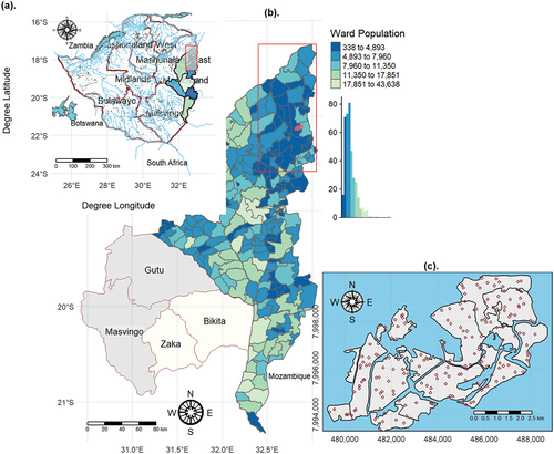
The study covered one of Zimbabwe’s commercial forests in Nyanga district in the eastern highlands of Zimbabwe. Apart from Pinus patula, Eucalyptus grandis and Eucalyptus camaldulensis as the major plantation forest tree species characterizing the studied region, substantial portions of the area has patches of land opened for agriculture and gold panning by neighboring farmers (European-Commission 2017). Our study area is located between longitude 32°40^’ E and 32°54^’ E and 18°10^’12^’’ S and 18°25^’4^’’ S latitude as illustrated in Figure 1. Grazing and gold panning activities in the neighborhood of the forest plantation started after the redistribution of some formerly owned commercial forest estates to peasant farmers in 2000 (Zvobgo and Tsoka 2021;). An area of approximately 2 767 ha is covered by the study area with variable rainfall amounts ranging from 741 mm to 2,997 mm and a mean annual precipitation of 1150 mm. The area experiences hot weather characterized by extensive wild veld fires around high-altitude grassland areas from September to November. Annual mean temperature range between 9°C and 12°C and 25°C and 28°C are experienced during the winter and summer seasons, respectively (ICAT 2022).

Figure 1. Map of the study area indicating (a) the province where samples were derived, (b) study area location within the particular province and (c) the spatial distribution of the sampled regionalized variable in the lower panel with points representing locations of sampled plots.

2.2. Data and pre-processing

2.2.1. Remote sensing data

The spatial coverage of remote sensing data such as the Landsat series and Sentinel-2, coupled with their easy and cheap availability provides immense opportunities for modeling natural resources of interest at relatively low cost. We make use of Landsat-8, Sentinel-2, WorldClim (Fick and Hijmans 2017) and the Shuttle Radar Topography Mission (SRTM) data to derive predictors for C stock prediction in a plantation forest ecosystem in the eastern highlands of Zimbabwe.

We obtained Landsat-8 Operational Land Imager (OLI) imagery data on the 20th of September 2020 from the Earth Explorer (http://earthexplorer.usgs.gov) website as a processed product ready for analysis. The dataset was rid of cloud cover with cloud shadow thresholds set to less than 10%. We also acquired the Sentinel-2 imagery covering the entire study area (lot 75A Nyanga Downs in the eastern highlands of Zimbabwe) at the same date and time that we acquired the Landsat-8 satellite data. Sentinel-2 data was obtained as level-1C 12-bit pre-set Top of the Atmosphere (TOA) reflectance values. We pre-processed and orthorectified Sentinel-2 1-C product in the R Statistical and Computing Environment using the sen2r library (Ranghetti et al. 2020). The Sentinel-2 sensor records data in 13 spectral bands with 4 in the visible range with 10 m spatial resolution, 6 in the near-infrared region with 20 m spatial resolution and 3 bands in the short-wave infrared region with a 60 m spatial resolution (Gerald et al. 2017). The same observation can therefore be imaged by a Landsat-8 and a Sentinel-2 satellite at varying spatial resolutions, spectral bandwidth and spectral response function. Landsat images downloaded from the United States Geological Survey (USGS) (http://earthexplorer.usgs.gov) are already orthorectified and projected.

2.2.2. Anthropogenic variables

The distance to settlements ($dist$) within the sampled region was utilized as an indicator of accessibility to forest resources by settlers within the plantation forest. Settlements were manually digitized using a combination of high-resolution Google Earth imagery and the revised 1:50 000 topographic maps covering the study area (Surveyor General 2018). We then calculated the distance to settlements from each of the sampled C stock plots for the Landsat-8 and Sentinel-2 satellite image data within a GIS environment. The need for modeling C stock with distance to settlements is based on the principle that accessibility to forest plantations exerts pressure on forest resources and increases the likelihood of direct and indirect impact on the planted forest (Chinembiri et al. 2013; Mon et al. 2012).

2.2.3. Climatic data

Because of the significant effect climatic conditions have on the density of AGB, we considered the Mean Annual Temperature (⁰ C) (MAT) and the Mean Annual Precipitation (mm) (MAP) in the modeling of C stock stretching a 30-year period from 1970 to 2000 from the WorldClim dataset (Fick and Hijmans 2017). WorldClim version 2.1 climatic data was provided at 30 arc seconds (~1 km) spatial resolution. Previous studies including MALHI et al. (2006) and Liu et al. (2014) have shown a significant association between MAT and MAP to forest biomass.

2.2.4. Topographic data

We derived elevation, slope and aspect data as the main topographic factors influencing forest biomass distribution (Su et al. 2016) from the Shuttle Radar Topography Mission (SRTM). We employed the 30 m SRTM digital elevation model (DEM) in deriving the aforementioned topographic variables. The SRTM covers approximately 99.96% of the global earth’s surface from 56° S to 60° N (Farr et al. 2007; Rabus et al. 2003). We reprojected all the datasets to a common grid reference system and rescaled to 1 km resolution using the nearest neighbor interpolation approach before bringing different multi-source data sets together (Christman and Rogan 2012). This was done in order to maintain consistency with the spatial resolution of the coarser dataset (1 km climatic dataset) and minimize error propagation during the data harmonization process (Robinson 1950).

2.2.5. Vegetation indices

We utilized Normalized Difference Vegetation Index ($NDVI$), Soil Adjusted Vegetation Index ($SAVI$), Enhanced Vegetation Index ($EVI$) derived from Landsat-8 and Sentinel-2 multispectral remote sensing data. The vegetation indices used in this study have also been applied as ancillary variables in literature (Bordoloi et al. 2022; Li and Li 2019) for biomass estimation because of their sound correlation with forest biophysical variables. Hence, we selected the broadband vegetation indices based on simplicity and robustness.

2.3. Methods

2.3.1. Uniform area spatial coverage sampling

Our C stock forest inventory data collection programme was done in an area with no history of sampling, implying lack of knowledge of scales of spatial variability. We therefore employed the k-means clustering algorithm for uniform area spatial coverage sampling that makes use of the Mean Squared Shortest Distance (MSSD) for optimization of sample locations (Brus, de Gruijter, and van Groenigen 2006; Walvoort, Brus, and de Gruijter 2010). As illustrated in Figure 1, even distribution of sampling locations across the sampling area enhances the estimation and mapping of regionalized variables (Walvoort, Brus, and de Gruijter 2010). Brus, de Gruijter, and van Groenigen (2006) demonstrated how even distribution of sample locations can be applied for estimating both spatial means and the resolution of mapping in environmental, forestry and soil science research. The suitability of the uniform area spatial coverage design also befits application in areas where sampling campaigns cannot be extended beyond the stipulated time frame.

2.3.2. Field sampling and tree biomass measurement

Sampling was done and measurements taken for all trees with at least 10 cm diameter at breast height (DBH) (1.3 m) using circular plots with an area of 500 m² between the 19^th of September 2021 and the 24^th of October 2021. Gibbs et al. (2007) suggest that individual trees with DBH measurements less than 10 cm store insignificant amounts of C stock. We did not consider slope correction during the tree biomass measurement exercise as the slopes in the studied region generally fall below 30% (Ravindranath and Ostwald 2008). Optimization of the sampling locations through uniform coverage sampling using the spcosa-library of the R Statistical and Computing Environment resulted in 200 samples (Brus, de Gruijter, and van Groenigen 2006). We pre-loaded the 200 samples into a 72 H handheld Garmin GPS before launching the field data collection programme and 191 samples of forest biomass measurements were used in the final analysis as the other nine samples fell outside the sampling region.

2.3.3. AGB calculation and C stock derivation

Three major plantation forest species, namely Pinus patula, Eucalyptus grandis and Eucalyptus camaldulensis are found in the study area. We therefore calculated the biomass of each of the tree species using specific allometric equations. Allometric equations by Brown (1997) were used for the calculation of the Pinus patula species tree biomass whilst we calculated the tree biomass for the Eucalyptus species using allometric equations by Zunguze (2012). The same allometric equations for the same tree species were utilized in the calculation of the Pinus and the Eucalyptus species biomass in Manica Province in Mozambique. Manica province of Mozambique closely resembles the climatic conditions of the studied region which it shares the same border in the eastern highlands of Zimbabwe. We then converted the AGB of each and every individual tree species to C stock using a conversion factor of the IPCC (2006). Per plot value estimates were then calculated to a MgCha⁻¹ standard AGB unit of measure.

2.3.4. Box-Cox transformation

An exploratory analysis of the target variable was done in order to evaluate the distribution properties of the modeled variable. The modeled C stock variable displayed distribution properties deviating from the required normality assumption and was therefore transformed using the appropriate transformation parameter as guided by Equation (1)(1) $\left\{Y\left(\lambda \right)=\begin{array}{c}(Y^{\lambda }-1)/\lambda if\lambda \ne 0\\ logYif\lambda =0\end{array}\right.$(1) (Box and Cox 1982).

(1) $\left\{Y\left(\lambda \right)=\begin{array}{c}(Y^{\lambda }-1)/\lambda if\lambda \ne 0\\ logYif\lambda =0\end{array}\right.$(1)

$Y$ denotes the target variable while $\lambda$ denotes the transformation parameter

The progress made by Box and Cox (1964) concerning the transformation parameter in Eqn 1 are of the normal linear model theory as in Equation (2)(2) $y\left(\lambda \right)=\mathit{X}\mathit{\beta }\left(\lambda \right)+\epsilon ,$(2) ,

(2) $y\left(\lambda \right)=\mathit{X}\mathit{\beta }\left(\lambda \right)+\epsilon ,$(2)

where $\mathit{X}$ denotes an $nxp$ vector of independent variables, $\mathit{\beta }\left(\lambda \right)$ is a $px1$ vector of unknown parameters while the standard deviation of the independent errors ${\epsilon }_i\left(i=1,\dots ,n\right)$ is $\sigma \left(\lambda \right)$. A 0.5 $\lambda$ entails a square root transformation, a $\lambda$ of 1 entails no transformation whilst a $\lambda$ of 0 supports a logarithmic transformation (Box and Cox 1964).

2.3.5. Bayesian hierarchical modeling

The model governing the relationship between the target C stock variable and the basket of multi-source predictors from the Landsat-8 and the Sentinel-2 satellite data was decomposed into a hierarchical structure (Gelfand 2012). The hierarchical structure is justified on the need to approach the complex relationship between the target variable and the multi-source predictor variables as a “total process” that can be decomposed into a data specification model (Equation (3)(3) $Y\left(s\right)={\mathit{x}}^T\left(s\right)\mathit{\beta }+w\left(s\right)+\epsilon \left(s\right)$(3) ), spatial random effects specification (Equation (4)(4) $w\sim MVN\left(0_s,{\sigma }_w^2{\mathrm{\Sigma }}_{\mathit{w}}\right)$(4) ) and the prior and hyperprior specification derived from the vector of parameters to be estimated. We therefore specified the Bayesian hierarchical model as in Equation (3)(3) $Y\left(s\right)={\mathit{x}}^T\left(s\right)\mathit{\beta }+w\left(s\right)+\epsilon \left(s\right)$(3) in order to have a full account of the parameter uncertainty of the measured C stock (Finley, Banerjee, and MacFarlane 2011).

(3) $Y\left(s\right)={\mathit{x}}^T\left(s\right)\mathit{\beta }+w\left(s\right)+\epsilon \left(s\right)$(3)

Where;

$Y\left(s\right)$ denotes the observed C stock data at a spatial location $s$,

$x\left(s\right)$ denotes a vector of predictors

$w\left(s\right)$ denotes a spatial process capturing the residual spatial association

$\mathit{\beta }$ denotes a vector of regression coefficients

$\epsilon \left(s\right)$ captures the random error (nugget effect) that is assumed $i.i.d.N\left(0,{\sigma }_{\epsilon }^2\right)$

We hypothesized the spatial random effects, $w\left(s\right)={\left(w,\dots ,w_s\right)}^T$, arises from a multivariate spatial distribution, that is, a normal random field, scaled by a spatial variance, ${\sigma }_w^2$, and correlations proportionate to the separation distance, $d_{ij}$, between sites as follows:

(4) $w\sim MVN\left(0_s,{\sigma }_w^2{\mathrm{\Sigma }}_{\mathit{w}}\right)$(4)

Where $0_s$ is an $Sx1$ vector of zeros, ${\sigma }_w^2$ denoting the between site variance and ${\mathrm{\Sigma }}_w$ is the $SxS$ correlation matrix with elements $\left(s_i,s_j\right)$ denoting the correlation between sites $s_i$ and $s_j$, $i,j=1,\dots ,S$.

Simultaneous estimation and prediction of the response variable parameters was made using the Markov Chain Monte Carlo (MCMC) algorithm for deriving and calculating the predictions of the primary variable at unsampled sites according to Equation (5)(5) $\hat{Y}{\left(s\right)}^{\prime }=X^T{\left(s\right)}^{\prime }\hat{\beta }+\hat{w}{\left(s\right)}^{\prime }.$(5) :

(5) $\hat{Y}{\left(s\right)}^{\prime }=X^T{\left(s\right)}^{\prime }\hat{\beta }+\hat{w}{\left(s\right)}^{\prime }.$(5)

We made the hierarchical modeling using the spBayes R Statistical and Computing Environment library (Finley, Sudipto, and Carlin 2007; R Core Development Team 2008). As discussed in Gelfand (2012), the Bayesian framework handles the vector of model parameters, $\mathit{\theta }=\mathit{\beta },{\sigma }^2,\varphi ,{\tau }^2$ (for the slope, structured dependence, the spatial decay parameter and the white noise, respectively) as random and mutually independent variables and assigns prior distributions to the parameters. The posterior distribution of parameters, $\mathit{\theta }$, was sampled in accordance with Equation (6)(6) $p\left(\mathit{\theta }|\mathit{y},X\right)\propto p\left(\mathit{\theta }\right)xN\left(\mathit{w}|0,{\mathrm{\Sigma }}_w\right)xN\left(\mathit{y}|X^t\mathit{\beta }+\mathit{w},{\mathrm{\Sigma }}_{\epsilon }\right)$(6) :

(6) $p\left(\mathit{\theta }|\mathit{y},X\right)\propto p\left(\mathit{\theta }\right)xN\left(\mathit{w}|0,{\mathrm{\Sigma }}_w\right)xN\left(\mathit{y}|X^t\mathit{\beta }+\mathit{w},{\mathrm{\Sigma }}_{\epsilon }\right)$(6)

Equation (6)(6) $p\left(\mathit{\theta }|\mathit{y},X\right)\propto p\left(\mathit{\theta }\right)xN\left(\mathit{w}|0,{\mathrm{\Sigma }}_w\right)xN\left(\mathit{y}|X^t\mathit{\beta }+\mathit{w},{\mathrm{\Sigma }}_{\epsilon }\right)$(6) was therefore employed in order to quantify the uncertainties in model parameter and predictions of the response variable at unvisited sites using the derivation in Equation (7)(7) $p\left(y_0|\mathit{y},\mathit{X},{\mathit{x}}_0\right)\propto \int p\left(y_0|\mathit{y},\mathit{\theta },{\mathit{x}}_0\right)p\left(\mathit{\theta }|\mathit{y},\mathit{X}\right)d\mathit{\theta }$(7) where the $y_0$ denotes predicted C stock at unsampled sites using covariates $x_0$ at site $s_0$.

(7) $p\left(y_0|\mathit{y},\mathit{X},{\mathit{x}}_0\right)\propto \int p\left(y_0|\mathit{y},\mathit{\theta },{\mathit{x}}_0\right)p\left(\mathit{\theta }|\mathit{y},\mathit{X}\right)d\mathit{\theta }$(7)

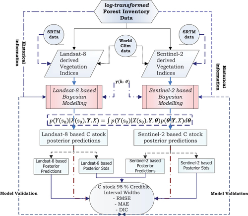
The study relied on a multi-source data supply from Landsat-8, Sentinel-2, climatic and topographic C stock related ancillary variables. Landsat-8 and Sentinel-2 multispectral remote sensing data formed the mainstream Bayesian hierarchical model building blocks where vegetation indices derived from them were integrated with anthropogenic, climatic and topographic variables from WorldClim (Fick and Hijmans 2017) and the SRTM data (Rabus et al. 2003). Two types of models were therefore constructed with prior specifications designated as $p\left({\mathit{\theta }}_1\right)$ and $p\left({\mathit{\theta }}_2\right)$ for the Landsat-8 and Sentinel-2-based C stock models, respectively.

We assigned the inverse gamma distribution for the data (C stock) and nugget variance whilst the spatial decay parameter was assigned a uniform prior. The maximum distance between the farthest sample locations $\left({\mathit{\theta }}_1,{\mathit{\theta }}_2\right)\in D$ in the studied area (2413 m) was used to guide assignment of the prior distribution of the spatial decay parameter. Scale parameters were assigned in order to convey the preference that the nugget error variance (${\sigma }_{\epsilon }^2$) $<$ the data variance (${\sigma }_w^2$) (Demirhan and Kalaylioglu 2015). We utilized the Metropolis-Hastings technique for the MCMC (Finley, Banerjee, and MacFarlane 2011). The technique is a type of a MCMC method that generates sequentially correlated draws from a sequence of probability distributions (Gelman 2006). We based the analysis on three chains of 11, 000 samples each where 1, 000 samples were discarded as part of burn-in. Subsequent analysis and parameter estimation therefore depended on the remaining 30, 000 (10, 000 × 3) samples. A summarized flow diagram of the data processing and handling using the Bayesian hierarchical approach is illustrated in Figure 2.

Figure 2. Multi-source data model prediction framework.

2.3.6. Bayesian geostatistical model validation

Each of the Landsat-8 and Sentinel-2-based spatial intercept only, independent error and the spatial models were evaluated for their prediction performance using a hierarchical modeling approach with $p\left({\mathit{\theta }}_1\right)$ and $p\left({\mathit{\theta }}_2\right)$ being used as guides for prior distribution specification as in Equations (8)(8) $p\left({\mathit{\theta }}_1\right)=\mathit{U}\mathit{n}\mathit{i}\mathit{f}\left(\varphi |0.39,0.0013\right)x\mathit{I}\mathit{G}\left({\sigma }^2|0.53,1.59\right)\text{break}x\mathit{I}\mathit{G}\left({\tau }^2|0.1,1.59\right)x\mathit{M}\mathit{V}\mathit{N}\left(\beta |0,{\mathrm{\Sigma }}_{\mathit{\beta }}\right)$(8) and (9(9) $p\left({\mathit{\theta }}_2\right)=\mathit{U}\mathit{n}\mathit{i}\mathit{f}\left(\varphi |0.39,0.0013\right)x\mathit{I}\mathit{G}\left({\sigma }^2|0.053,0.0029\right)\text{break}x\mathit{I}\mathit{G}\left({\tau }^2|0.1,1.53\right)x\mathit{M}\mathit{V}\mathit{N}\left(\beta |0,{\mathrm{\Sigma }}_{\mathit{\beta }}\right)$(9) ):

(8) $p\left({\mathit{\theta }}_1\right)=\mathit{U}\mathit{n}\mathit{i}\mathit{f}\left(\varphi |0.39,0.0013\right)x\mathit{I}\mathit{G}\left({\sigma }^2|0.53,1.59\right)\text{break}x\mathit{I}\mathit{G}\left({\tau }^2|0.1,1.59\right)x\mathit{M}\mathit{V}\mathit{N}\left(\beta |0,{\mathrm{\Sigma }}_{\mathit{\beta }}\right)$(8)

(9) $p\left({\mathit{\theta }}_2\right)=\mathit{U}\mathit{n}\mathit{i}\mathit{f}\left(\varphi |0.39,0.0013\right)x\mathit{I}\mathit{G}\left({\sigma }^2|0.053,0.0029\right)\text{break}x\mathit{I}\mathit{G}\left({\tau }^2|0.1,1.53\right)x\mathit{M}\mathit{V}\mathit{N}\left(\beta |0,{\mathrm{\Sigma }}_{\mathit{\beta }}\right)$(9)

$p\left({\theta }_1\right)$ and $p\left({\mathit{\theta }}_2\right)$ are prior specifications assigned using values of an exploratory variogram of the C stock model of feature space derived from the Landsat-8 and the Sentinel-2 derived covariates, respectively. The uniform distribution, the inverse gamma distribution and the multivariate normal distribution are specified in Equations (8)(8) $p\left({\mathit{\theta }}_1\right)=\mathit{U}\mathit{n}\mathit{i}\mathit{f}\left(\varphi |0.39,0.0013\right)x\mathit{I}\mathit{G}\left({\sigma }^2|0.53,1.59\right)\text{break}x\mathit{I}\mathit{G}\left({\tau }^2|0.1,1.59\right)x\mathit{M}\mathit{V}\mathit{N}\left(\beta |0,{\mathrm{\Sigma }}_{\mathit{\beta }}\right)$(8) and (9(9) $p\left({\mathit{\theta }}_2\right)=\mathit{U}\mathit{n}\mathit{i}\mathit{f}\left(\varphi |0.39,0.0013\right)x\mathit{I}\mathit{G}\left({\sigma }^2|0.053,0.0029\right)\text{break}x\mathit{I}\mathit{G}\left({\tau }^2|0.1,1.53\right)x\mathit{M}\mathit{V}\mathit{N}\left(\beta |0,{\mathrm{\Sigma }}_{\mathit{\beta }}\right)$(9) ) with $\mathit{U}\mathit{n}\mathit{i}\mathit{f}$, $\mathit{I}\mathit{G}$ and $\mathit{M}\mathit{V}\mathit{N}$ notations, respectively.

A $k-$fold cross validation algorithm was used for evaluating the predictive performance of each of the spatial intercept only, error independent and the spatial models by random splitting of the 191 sampled C stock data into 10 equally sized segments (Duchene et al. 2016). The spatial intercept only model considers only the model intercept (slope) and the spatial locations of the sampled variable whilst the independent error model only models the target variable and the predictors without the covariates. On the other hand, the spatial model takes into consideration the spatial location of the modelled variable (Sahu 2022). The Root Mean Square Error ($RMSE$) and the Mean Absolute Error ($MAE$) in addition to other goodness of fit metrics were calculated and used as ranking criteria for models’ ability in fitting the data (Spiegelhalter et al. 2002). Models regarded as better fitting have lower values of the Deviance Information criterion ($DIC$) whilst top performing models have the smallest $k\left(k=10\right)$ fold $RMSE$ and $MAE$ statistics. Graphical trace plots were also used as diagnostics for assessing the adequacy of modeling assumptions (Green, Finley, and Strawderman 2020; Jackman 2000).

2.3.7. Predictive model uncertainty assessment

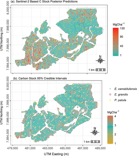
Multi-source predictor variables utilized in the Landsat-8 and Sentinel-2 driven C stock models were assessed for significance using the 2.5% and the 97.5% posterior sample percentiles. Independent variables in the hierarchical models were certified significant if their 95% Credible Intervals (CIs) did not contain zero, with uncertainty being assessed according to Hengl et al. (2004) method. We displayed the median predictions of C stock for each grid cell (100 m × 100 m), using a color ramp together with the associated 95% Credible Interval Widths (CIWs). Predictions with higher uncertainties have wider CIWs (Babcock et al. 2016, 2018).

3. Results

The objective Box-Cox transformation approach for the target variable (C stock) as detailed in Equation (1)(1) $\left\{Y\left(\lambda \right)=\begin{array}{c}(Y^{\lambda }-1)/\lambda if\lambda \ne 0\\ logYif\lambda =0\end{array}\right.$(1) gave a lambda ($\lambda )$ value of 0.012. This transformation parameters led to a log transformation of the modelled C stock variable.

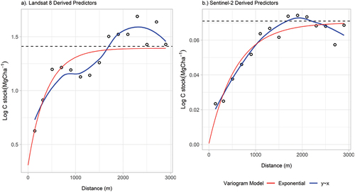
The spatial correlation structure of Landsat-8 and Sentinel-2-based C stock models build from a WorldClim and SRTM multi-source supply of predictors saw the Sentinel-2-based C stock prediction model with the longest mean effective range (2000 m) compared to its Landsat-8 (1500 m) counterpart (Figure 3). Greater influence of the Sentinel-2 driven C stock model manifests through the spatial covariance structure in which its spatially structured variance (${\sigma }_{\mathit{w}}^2$ = 0.589) is much reduced than that of the Landsat-8 driven C stock model (${\sigma }_{\mathit{w}}^2$ = 1.21). This trajectory also holds true for the micro-scale variance in both models. However, the Landsat-8 C stock-based model has lower effective range (1500 m) when compared to the Sentinel-2-based C stock model due to the vanishing spatial structure in the latter.

Figure 3. Multi-source variogram of residuals for the Landsat-8 and sentinel-2 driven C stock models. Asymptotes for the theoretical variogram models are illustrated with a black dotted line.

3.1. The influence of multi-source predictor variables on C stock

A multi-source prediction of C stock using topographic, climatic, anthropogenic and vegetation indices show distance to settlements ($DIST$) and $NDVI$ as the only significant predictors (Table 1) for both Landsat-8 and Sentinel-2 C stock models. The effect of $NDVI$ is much stronger in Sentinel-2 than in Landsat-8-based C stock model, justifying from the higher spatial resolution of Sentinel-2. The 95% credible intervals of all the topographic ($aspect$, $slope$ and $elevation$) and climatic ($MAP$ and $MAT$) explanatory variables contain zero and hence, not significant predictors of C stock for both the Landsat-8 and the Sentinel-2 models.

Table 1. Landsat-8 and sentinel-2-based C stock model parameter estimates. $DIST$ is distance to settlements, $MAT$ is mean annual temperature, $MAP$ is mean annual rainfall.

Parameter classification	Parameter	Landsat-8 C stock Model	Sentinel-2 C stock Model
		50% (2.5%, 97.5%)	50% (2.5%, 97.5%)
Intercept	$Intercept$	−43.8 (16.36, 75.0)	−6.8 (−36.1, 22.3)
Vegetation indices	$NDVI$	2.58 (0.52, 4.76)	4.95 (4.49, 5.44)
	$SAVI$	−0.07 (−1.39, 1.32)	−0.94 (−1.66, −0.20)
	$EVI$	−0.49 (−1.59, 0.63)	0.11 (−0.07, 0.30)
Anthropogenic	$DIST$	1.42 (0.75, 2.09)	0.82 (0.55, 1.07)
Topographic	$Elevation$	0.001 (−0.003, 0.005)	0.0004 (−0.0004, −0.0001)
	$Slope$	−0.069 (1.00, 0.87)	0.08 (−0.27, 0.43)
	$Aspect$	−0.41 (−0.89, 0.085)	0.05 (−0.04, 0.14)
Climatic	$MAT$	−0.60 (−3.07, 1.84)	−0.12 (−0.62, 0.38)
	$MAP$	−0.047 (−0.26, 0.16)	−0.02 (−0.07, 0.03)
Spatial covariance	${\sigma }_w^2$	1.21 (0.71, 1.87)	0.0589 (0.045, 0.075)
	${\sigma }_{\epsilon }^2$	0.33 (0.062, 0.65)	0.0024 (0.0007, 0.0076)
	$\varphi$	0.002 (0.002, 0.003)	0.0015 (0.0014, 0.0021)
	$Effectiverange\left(m\right)$	1500 (1000, 1500)	2000 (1428, 2143)

However, $SAVI$ is a significant predictor in the Sentinel-2-based C stock model whilst its 95% CI (−1.39, 1.32) contains zero in the Landsat-8-based model (Table 1). Vegetation indices are dominant over other predictor categories like climate and topography in both new generation multispectral remote sensing-based C stock prediction models. The predicted C stock therefore represents averaged pixel values as predictor variables were gridded on a 10 000 m² resolution raster surface. A total of 30 000 samples for each grid were obtained from the MCMC sampling from the fitted models’ predictive distribution. There is evidently weaker spatial correlation from the Landsat-8 driven C stock prediction model with a mean effective range of 1500 m and an associated 95% CI of (1000, 1500) m compared to the Sentinel-2-based C stock model showing a much stronger spatial correlation having a mean effective range of 2000 m and an associated (1428, 2143) m 95% CI (Table 1).

3.2. Landsat-8 and sentinel-2-based multi-source C stock prediction

Different spectral properties of new generation remote sensing Landsat-8 and Sentinel-2 represent different potential and capabilities for predicting natural resource variables of interest in climate change studies.

Comparison of the models constructed from vegetation indices derived from these sensors alongside other ancillary climatic and topographic information using Bayesian hierarchical modeling shows $NDVI$ and distance to settlements ($DIST$) as significant predictors of C stock in both models. As explained in the subsequent sections, other climatic and topographic class of predictor variables have no influence on C stock prediction (Table 1).

3.2.1. Landsat-8-based C stock model

Anthropogenic and vegetation spectral index-based Landsat-8 prediction model gave C stock prediction range between 1 MgCha⁻¹ and 135 MgCha⁻¹ with a 95% CI range of $2\le MgCh{a}^{-1}\le 4$ (Figure 4).

Figure 4. (a) Posterior mean and (b) standard deviation of the Landsat-8-based C stock model. The points in the figure represents C stock plot locations for the three different tree species.

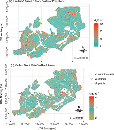
C stock prediction uncertainty is relatively non-uniform across the studied region as can be shown by occurrence of red pixels representing high C stock prediction uncertainty. There is a notable trend of higher C stock predictions in the northern, western and central parts of the studied region which can be attributed to timber plantation accessibility and illegal logging activities from nearby resettled farmers (Figure 4).

3.2.2. Sentinel-2-based C stock predictions

The same trend of higher C stock predictions in the northern, western and central regions of the study area is present in Sentinel-2-based C stock prediction model (Figure 5). In addition to distance to settlements and $NDVI$ as driving predictors of the C stock, the Sentinel-2 C stock model also carries $SAVI$ as a significant predictor, predicting the resource variable with a range between 1 MgCha⁻¹ and 130 MgCh⁻¹ as illustrated in Figure 5. However, despite the higher spatial and spectral resolution in Sentinel-2 derived vegetation indices, the Sentinel-2-based C stock model displays higher posterior uncertainty ($1\le MgCh{a}^{-1}\le 4$) compared to that of Landsat-8 (Figure 4).

Figure 5. (a) Posterior mean and (b) standard deviation of the sentinel-2-based C stock model. The points in the figure represents C stock plot locations for the three different tree species.

3.3. C stock model prediction performance assessment

A comparison of the prediction performance of the Landsat-8 and Sentinel-2-based C stock models favor the latter as it has lower RMSE (1.17 MgCha⁻¹) compared to its Landsat-8-based C stock (2.16 MgCha⁻¹) counterpart (Table 2). The Sentinel-2-based C stock model also fits the data well as it displays far much lower Deviance Information Criteria (DIC) (−554.7) than the Landsat-8-based C stock (43.1) model. Different variants of the Bayesian prediction models with different levels of specifications (non-spatial, spatial and error independent models) for both the Landsat-8 and the Sentinel-2 models favor the C stock model with full spatial specifications (Table 2).

Table 2. C stock model performance validation statistics.

Model Validation criterion	Landsat 8-based C Stock Model			Sentinel-2-based C Stock Model
	Independent Error Model	Spatial Intercept only Model	Spatial Model	Independent Error Model	Spatial Intercept only Model	Spatial Model
$RMSE$ (MgCha^−1)	3.06	2.08	2.16	1.31	2.89	1.17
$MAE$ (MgCha^−1)	2.36	1.43	1.55	1.22	1.97	1.13
$CRPS$ (MgCha^−1)	2.01	1.49	1.52	1.20	1.77	1.14
$CVG$ (%)	91.7	85.4	85.4	95.8	89.6	94.7
$DIC$	210.2	56.9	43.1	207.9	37.8	−554.7

The Landsat-8-based C stock model has slightly more under predictions and over predictions and less coverage (93.8%) than the Sentinel-2-based C stock model (97.9%) (Figure 6). Our definition of coverage in this study resonates with the definition provided by (Guhaniyogi and Banerjee (2019) as the proportion of reliably predicted C stock within the studied region of interest.

Figure 6. Landsat-8-based predicted C stock ($MgCh{a}^{-1}$) against C stock observations ($MgCh{a}^{-1}$) alongside 95% CIs.

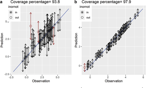
As such, the Landsat-8-based C stock model’s 93.8% coverage provides predictive ability slightly short of the nominal benchmark 95% coverage level whilst the Sentinel-2 C stock model is slightly above (97.9%).

3.4. MCMC convergence diagnostic assessment

$NDVI$ and $DIST$ in addition to the model intercept prediction MCMC trace plots are illustrated in Figure 7. The trace plots are provided as visual aides for assessing MCMC chain convergence and it is evident from Figure 7 that the length $N_0$, of the burin-in duration allowed Markov chain convergence to the stationary distribution as they were sufficiently large. Presentations shown are as a result of chain thinning for improving the aesthetic look of the plots.

Figure 7. Landsat-8 and sentinel-2-based C stock prediction MCMC trace plots.

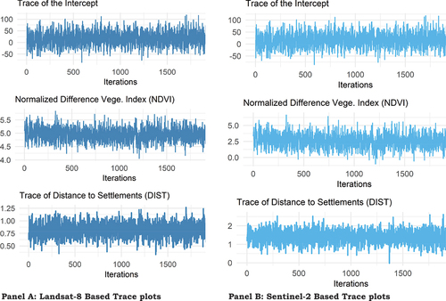
Thinning speeds up calculations by reducing the Monte Carlo sample size and the chains appear to have sufficiently converged to the stationary distribution and mix fairly well after 5, 000 (1500 after thinning) iterations. An assessment of Figure 7 shows a converged sample with MCMC with satisfactory mixing.

4. Discussion

The work we present in this study illustrates the importance of coupling different sources of earth observation data in addressing C stock dynamics in managed plantation forest ecosystems. We adopted a multi-source data approach to the prediction of C stock in a disturbed plantation forest ecosystem using anthropogenic, climatic and topographic derived explanatory variables using Landsat-8 and Sentinel-2 as the mainstream modeling drivers. Literature is replete with AGB and climate change related studies adopting statistical inferential methods utilizing a combination or stand alone machine learning and remote sensing approaches (Do et al. 2022; González-Vélez et al. 2021; Zhang et al. 2023).

Landsat-8 and Sentinel-2 are equally comparable multispectral remote sensing data sources, but their spatial and spectral properties, coupled with vegetation related climatic and topographic covariates is a good ground for assessing their suitability in C stock assessment for climate change implementation and action plans.

4.1. The influence of multi-source predictors on C stock dynamics

The finer spatial resolution of the Sentinel-2 (10 m) satellite data coupled with a supply of other predictors from the WorldClim and the SRTM have stronger explanatory properties than the ones used in Landsat-8 OLI data. Patches of sparsely forested areas are common in the study area due to illegal logging, agricultural activities and overgrazing, which makes $SAVI$ significant in Sentinel-2-based C stock model than in the Landsat-8 OLI C stock model (Somvanshi and Kumari 2020). Modelled topographic variables including elevation are not significant predictors of C stock in the model due to insignificant gradient changes in the study area. Consequently, the spatial variability (Baccini et al. 2004) in the sampled region is not good enough to influence vegetation dynamics. It seems the effect of elevation will be much evident when the study is done on a larger scale (regional rather than local scale) (Su et al. 2016). Both climatic variables, that is, MAP and MAT are not insignificant predictors of C stock in this study. This could be an indication of small to insignificant variability of the factors in the studied area due to its localized spatial extent vis regional scale studies done by Simard et al. (2019) and Jiang et al. (2021). Temperature and rainfall usually vary at landscape rather than at local scales (Zhang et al. 2023). Resettled farmers from the agrarian land reform most likely exploit forest resources closer to their settlements and which can easily be accessed due to closeness to roads and grazing facilities. As the results of C stock predictions show, it is within the same areas of higher C stock predictions that there is higher posterior uncertainty of C stock as a result of the plantation forest possibly responding to multi-sources of environmental variability.

As provided by Isaaks and Srivastava (1989), geostatistical predictions are plausible as prediction uncertainty is lower near sampled C stock observations. On the other hand, the significance of $NDVI$ as an index correlated with forest biophysical attributes, amongst them, chlorophyll and leaf area index ($LAI$) is much established (Baugh and Groeneveld 2006). Higher C stock prediction uncertainty associated with the Sentinel-2-based C stock model indicates modeling inadequacy in terms of the full complement of auxiliary variables needed for capturing C stock variability in the study area. This is because the advanced spatial and spectral resolution of Sentinel-2 derived data suggest that Sentinel-2-based models perform better than the Landsat-8 models (Semela, Ramoelo, and Adelabu 2020). The fact that all the other topographic and climatic variables are irrelevant in the prediction of C stock in either the Landsat-8 or the Sentinel-2-based C stock models imply $DIST$ and $NDVI$ are the major but inadequate sources of spatial variability for C stock prediction in the region. However, prediction uncertainty of Sentinel-2-based C stock model looks uniform and less variable across the study domain compared to that in the Landsat-8-based C stock prediction model. Better spectral properties in Sentinel-2 (13 spectral bands) compared to the Landsat-8 (11 spectral bands) seem to justify the quality of C stock predictions in both models (Azevedo 2021; Jia et al. 2014).

4.2. Multi-source C stock prediction modeling

In spite of coupling different data sources for C stock prediction in a plantation forest ecosystem set-up, vegetation spectral indices and anthropogenic ($DIST$) covariables emerge as significant predictors of C stock. Bordoloi et al. (2022) and Somvanshi and Kumari (2020) showed $NDVI$, $SAVI$ and $EVI$ as significant regressors of AGB in a Landsat-8 and Sentinel-2-based remote sensing framework. However, studies coupling new generation remote sensing information in a multi-source data approach using Bayesian hierarchical modeling are not common. Furthermore, studies that have implemented a multi-source data approach using other approaches like machine learning (SVM, boosted regression trees and multiple regression splines) have established lower prediction accuracies (8–13 Mgha⁻¹) than the present study (between 1.31 MgCha⁻¹ and 1.17 MgCha⁻¹) (Serrano et al. 2019; Shi, Liu, and Tumuluru 2017). Prediction accuracy differences between similar studies in literature and our study can be justified by the unmatched flexibility of the Bayesian inferential approach in partitioning sources of error and providing access to the entire posterior predictive distribution, which other inferential techniques cannot do (Beloconi and Vounatsou 2020; Goulard and Voltz 1992). The present study went a step further by comparing the performance of C stock models constructed using different multispectral remote sensing platforms within a Bayesian framework and established Sentinel-2 as the best performing C stock model.

A study by Chinembiri et al. (2023a) using a combination of anthropogenic and vegetation spectral indices within a Bayesian hierarchical framework using Landsat-8 and Sentinel-2 as the main data sources gave prediction accuracies with RMSE of 1.16 MgCha⁻¹ and 2.69 MgCha⁻¹ respectively. This study did not comprehensively deal with all the possible AGB sources of variation including climatic variables. However, adoption of a multi-source data approach using the same multispectral remote sensing data sources in the present study resulted in prediction accuracies with RMSE of 1.17 MgCha⁻¹ and 2.16 MgCha⁻¹ for the Landsat-8 and the Sentinel-2-based C stock models respectively. It is therefore evident that Sentinel-2 remote sensing is a promising and valuable AGB prediction remote sensing ancillary data source as it provides relatively lower prediction uncertainty (2.16 MgCha⁻¹) than its Landsat-8 (1.16 MgCha⁻¹) counterpart. The importance of multi-source data coupling within a Bayesian approach for C stock modeling in climate change studies is notable and has the potential for supplying the much needed answers to climate change implementation and mitigation strategies.

4.2.1. Climatic variables and C stock prediction

Contrary to global climate change studies, neither MAP nor MAT are significant covariates for C stock prediction in the present study. The influence of climate on C storage and distribution in global forests is well established (Pan et al. 2013). The constraints that precipitation and temperature exert on biomass production clearly link them to biomass storage (Keith, Mackey, and Lindenmayer 2009; Pan et al. 2013). Temperature controls carbon dioxide assimilation rates in the leaves (Lloyd and Farquhar 1996) and C losses from respiration related to living tissue maintenance (Larjavaara and Muller-Landau 2012). An inverse relationship between elevation and AGB is well established, for example, AGB is high at low elevations since these regions have high temperature, thick air and weak ultraviolet rays that promote vegetative growth of plants (Ahmed, Atzberger, and Zewdie 2022). On the other hand, changes in aspect and slope effect on forest biomass is associated with changes in soil nutrients and climatic conditions in small areas (Jucker et al. 2018). Again, areas with gentle slopes have excellent nutrition and soil moisture conditions making the AGB in these environments significantly higher than in poor and steep soils (He et al. 2022).

It appears there is less spatial variability of MAP as one moves from one geo-location to the other within the studied region (Gordon et al. 2018). However, the spatio-temporal influence of MAP also need to be investigated as it plays a pivotal role in AGB dynamics (Simard et al. 2019). This is the same explanation with MAT. This variable does not change dramatically over short distances, but over bigger distances. The maximum distance between the farthest sampling points within the study area is approximately 2500 m, making it inconceivable to expect significant temperature or precipitation changes (Chinembiri, Mutanga and Dube, 2023b). However, elevation can dramatically change over short distances, depending on the topography of the area, but it appears the studied area has a generally uniform landscape not complicated enough to influence C stock dynamics of the region.

The multi-source range of predicted C stock values for plantation forest with Pinus patula, Eucalyptus grandis and Eucalyptus camaldulensis as the dominant species for the current study is for the Landsat-8-based C stock model and $1\le MgCh{a}^{-1}\le 130$ for the Sentinel-2-based C stock prediction model. An assessment of AGB distribution of a Vietnamese mangrove forest using a combination of Artificial Neural Network (ANN) and remote sensing data resulted in a mangrove AGB prediction range of ($6.53-368.2$) Mgha⁻¹ in 2000 and from ($13.75-320.3$) Mgha⁻¹ in 2020, respectively (Do et al. 2022). AGB predictions established by Fararoda et al. (2021) using AdaBoost, random decision forest, multilayer neural networks and Bayesian ridge regression machine learning methods recommended AdaBoost and random forest as the best performing methods. The type of remote sensing platform together with the method of prediction employed have significant sway over AGB model performance (Ahmed, Atzberger, and Zewdie 2022). For instance, Fassnacht et al. (2014) assessed and compared hyperspectral and LiDAR data for AGB modeling and noted that Random forest models fused with LiDAR data offers the best AGB model prediction performance. The best model predictions are derived using a combination of the modeling methodology and a near complete coverage of all possible sources of spatial variability of the modelled variable. We endeavored to meet these two conditions by employing the novel Bayesian hierarchical approach with a multi-source supply of predictor variables. However, the limitation in our endeavors appear to be the complex spatio-temporal dynamics between AGB and MAP and MAT coupled with scale, as the studied region is rather small to trigger meaningful C stock variability (Ahmed, Atzberger, and Zewdie 2022; Baccini et al. 2004).

Prediction accuracies in our study seem superior than accuracies established in similar studies and environments, implying the results of this study can be applied in comprehensive and targeted ecosystem intervention (Ahmed, Atzberger, and Zewdie 2022; Fan, Wang, and Yang 2022; Jiang et al. 2021; Takagi et al. 2015; Xiong and Wang 2022). Improvement in the spatial and spectral properties of Sentinel-2 as realized from the model’s Credible Interval width (CIWs) makes it the best data source for forest resource monitoring within the United Nations Framework Convention on Climate Change (UNFCCC). This implies that conservation and monitoring of extensive plantation forest ecosystems can be achieved with higher precision and accuracy and consequently, improve forest carbon accounting.

5. Conclusions

We undertook to predict C stock in a managed and disturbed plantation forest ecosystem in the eastern highlands of Zimbabwe using a multi-source data approach coupling forest inventory data with remote sensing derived information in a Bayesian geostatistical hierarchical framework. Forest productivity related multi-data sources based on anthropogenic, climatic and topographic factors were utilized as predictors of C stock, with Landsat-8 and Sentinel-2 as the mainstream model building blocks. Unlike in other studies that have been done at landscape scale, both climatic and topographic variables were not significant predictors of C stock. An $NDVI$ and $DIST$ driven Sentinel-2 C stock model with a prediction RMSE of 1.17 MgCha⁻¹ outperformed its Landsat-8 model counterpart with a 2.16 MgCha⁻¹ RMSE. A multi-source data approach of C stock modeling at a local scale does not improve prediction uncertainty in plantation forests, but the Sentinel-2 constructed C stock model provides lower prediction uncertainty than its Landsat-8 counterpart.

A more practical model for use by forest practitioners and subsequent adoption by central governments is the one based on Sentinel-2-based data with $NDVI$ and $DIST$ as drivers of C stock variability. The need for accurate accounting of C stock density and assessment of C sequestration potential in both natural and plantation forests by national governments under the UNFCCC requires construction of credible and error free models. The dynamics between the ability of communities to access forestry resources and services and the rate of C sequestration is critical for site specific interventions needed for ecological monitoring and ecosystem restoration. The Bayesian approach together with free and analysis ready Sentinel-2 data is particularly handy as it nearly eliminates the need for extensive forest inventory surveys that may be needed at frequent intervals for C accounting for climate change strategies and mitigation plans. Essentially, today’s C stock posterior predictions will be the basis for future C stock modeling as C stock model priors.

Author contributions

Writing – original draft, T.S.C.; Writing – review & editing, T.D.; Review of manuscript, project administration and funding, O.M. All authors have read and agreed to the published version of the manuscript.

Acknowledgments

The authors wish to express their sincere gratitude to Kutsaranga, Matowanyika and Mukwekwe for providing authority and means to access the plantation forest used as sampling area at Lot 75A of Nyanga Downs in the eastern highlands. This study received support from the University of KwaZuluNatal, college of Agricultural, Earth and Environmental Science.

Disclosure statement

No potential conflict of interest was reported by the author(s).

Additional information

Funding

This work is based on the research supported in part by the National Research Foundation of South Africa [Grant Number: 84157].

References

- Ahmed, N., C. Atzberger, and W. Zewdie. 2022. “The Potential of Modeling Prosopis Juliflora Invasion Using Sentinel-2 Satellite Data and Environmental Variables in the Dryland Ecosystem of Ethiopia.” Ecological Informatics 68:101545. https://doi.org/10.1016/j.ecoinf.2021.101545.
- Ali, A., S.-L. Lin, J.-K. He, F.-M. Kong, J.-H. Yu, and H.-S. Jiang. 2019. “Climate and Soils Determine Aboveground Biomass Indirectly via Species Diversity and Stand Structural Complexity in Tropical Forests.” Forest Ecology and Management 432:823–21. https://doi.org/10.1016/j.foreco.2018.10.024.
- Álvarez-Dávila, E., L. Cayuela, S. González-Caro, A. M. Aldana, P. R. Stevenson, O. Phillips, Á. Cogollo, et al. 2017. “Forest Biomass Density Across Large Climate Gradients in Northern South America is Related to Water Availability but Not with Temperature.” PLoS One 12 (3): e0171072. Public Library of Science San Francisco, CA USA. https://doi.org/10.1371/journal.pone.0171072.
- Azevedo, L. 2021. “Model Reduction in Geostatistical Seismic Inversion with Functional Data Analysis Geophysics.” Society of Exploration Geophysicists 87 (1): M1–M11. https://doi.org/10.1190/geo2021-0096.1.
- Babcock, C., A. O. Finley, H.-E. Andersen, R. Pattison, B. D. Cook, D. C. Morton, M. Alonzo, et al. 2018. “Geostatistical Estimation of Forest Biomass in Interior Alaska Combining Landsat-Derived Tree Cover, Sampled Airborne Lidar and Field Observations.” Remote Sensing of Environment 212:212–230. https://doi.org/10.1016/j.rse.2018.04.044.
- Babcock, C., A. O. Finley, B. D. Cook, A. Weiskittel, and C. W. Woodall. 2016. “Modeling Forest Biomass and Growth: Coupling Long-Term Inventory and LiDAR Data.” Remote Sensing of Environment 182:1–12. https://doi.org/10.1016/j.rse.2016.04.014.
- Baccini, A., M. A. Friedl, C. E. Woodcock, and R. Warbington. 2004. “Forest biomass estimation over regional scales using multisource data.” Geophysical Research Letters 31 (10). John Wiley & Sons, Ltd. https://doi.org/10.1029/2004GL019782.
- Banerjee, S., B. P. Carlin, and A. E. Gelfand. 2003. Hierarchical Modeling and Analysis for Spatial Data. Chapman and Hall/CRC.
- Baugh, W. M., and D. P. Groeneveld. 2006. “Broadband Vegetation Index Performance Evaluated for a Low‐Cover Environment.” International Journal of Remote Sensing 27 (21): 4715–4730. https://doi.org/10.1080/01431160600758543.
- Beloconi, A., and P. Vounatsou. 2020. “Bayesian Geostatistical Modelling of High-Resolution NO2 Exposure in Europe Combining Data from Monitors, Satellites and Chemical Transport Models.” Environment International 138:105578. https://doi.org/10.1016/j.envint.2020.105578.
- Bordoloi, R., B. Das, O. P. Tripathi, U. K. Sahoo, A. J. Nath, S. Deb, D. J. Das, et al. 2022. “Satellite Based Integrated Approaches to Modelling Spatial Carbon Stock and Carbon Sequestration Potential of Different Land Uses of Northeast India.” Environmental and Sustainability Indicators 13:100166. https://doi.org/10.1016/j.indic.2021.100166.
- Box, G. E. P., and D. R. Cox. 1964. “An Analysis of Transformations (With Discussion).” Journal of the Royal Statistical Society: Series B (Methodological) 26 (2): 211–243. https://doi.org/10.1111/j.2517-6161.1964.tb00553.x.
- Box, G. E. P., and D. R. Cox. 1982. “An Analysis of Transformations Revisited, Rebutted.” Journal of the American Statistical Association 77 (377): 209–210. https://doi.org/10.1080/01621459.1982.10477788.
- Brown, S. 1997. FAO Forestry Paper, 134. Rome: FAO - Food and Agriculture Organization of the United Nations.
- Brus, D. J., J. J. de Gruijter, and J. W. van Groenigen. 2006. “Chapter 14 Designing Spatial Coverage Samples Using the K-Means Clustering Algorithm.” Developments in Soil Science 31:183–192. https://doi.org/10.1016/S0166-2481(06)31014-8.
- Chinembiri, T. S., M. C. Bronsveld, D. G. Rossiter, and T. Dube. 2013. “The Precision of C Stock Estimation in the Ludhikola Watershed Using Model-Based and Design-Based Approaches.” Natural Resources Research 22 (4): 297–309. https://doi.org/10.1007/s11053-013-9216-6.
- Chinembiri, T. S., O. Mutanga, and T. Dube. 2023a. “Carbon Stock Prediction in Managed Forest Ecosystems Using Bayesian and Frequentist Geostatistical Techniques and New Generation Remote Sensing Metrics.” Remote Sensing 15 (6): 1649. https://doi.org/10.3390/rs15061649.
- Chinembiri, T. S., O. Mutanga, and T. Dube. 2023b. “Hierarchical Bayesian Geostatistics for C Stock Prediction in Disturbed Plantation Forest in Zimbabwe.” Ecological Informatics 73:101934. https://doi.org/10.1016/j.ecoinf.2022.101934.
- Christman, Z. J., and J. Rogan. 2012. “Error Propagation in Raster Data Integration: Impacts on Landscape Composition and Configuration.” Photogrammetric Engineering & Remote Sensing 78 (6): 617–624. https://doi.org/10.14358/PERS.78.6.617.
- Cressie, N., and C. K. Wikle. 2011. Statistics for Spatio-Temporal Data. John Wiley and Sons.
- Demirhan, H., and Z. Kalaylioglu. 2015. “Joint Prior Distributions for Variance Parameters in Bayesian Analysis of Normal Hierarchical Models.” Journal of Multivariate Analysis 135:163–174. https://doi.org/10.1016/j.jmva.2014.12.013.
- Do, A. N. T., H. D. Tran, M. Ashley, and A. T. Nguyen. 2022. “Monitoring Landscape Fragmentation and Aboveground Biomass Estimation in Can Gio Mangrove Biosphere Reserve Over the Past 20 Years.” Ecological Informatics 70:101743. https://doi.org/10.1016/j.ecoinf.2022.101743.
- Duchene, S., D. A. Duchêne, F. Di Giallonardo, J.-S. Eden, J. L. Geoghegan, K. E. Holt, S. Y. W. Ho, et al. 2016. “Cross-Validation to Select Bayesian Hierarchical Models in Phylogenetics.” BMC Evolutionary Biology 16 (1). https://doi.org/10.1186/s12862-016-0688-y.
- Eamus, D. 2003. “How Does Ecosystem Water Balance Affect Net Primary Productivity of Woody Ecosystems?” Functional Plant Biology 30 (2): 187–205. https://doi.org/10.1071/FP02084.
- European-Commission. 2017. Timber Trade Flows Within, to and from Eastern and Southern African Countries. Brussels: European Commission.
- Fang, J., A. Chen,C. Peng,S. Zhao, and L. Ci. 2001. “Changes in Forest Biomass Carbon Storage in China Between 1949 and 1998.” Science American Association for the Advancement of Science 292 (5525): 2320–2322. https://doi.org/10.1126/science.1058629.
- Fan, M., X. Wang, and G. Yang. 2022. “Spatial Characteristics of Vegetation Habitat Suitability and Mountainous Settlements and Their Quantitative Relationships in Upstream of Min River, Southwestern of China.” Ecological Informatics 68:101541. https://doi.org/10.1016/j.ecoinf.2021.101541.
- FAO. 2003. Forestry Outlook Study for Africa. Regional Report - Opportunities and Challenges Towards 2020. Rome, Italy.
- FAO. 2016. Global Forest Resources Assessment. Howare the World’s Forests Changing? Rome, Italy: FAO - Food and Agriculture Organization of the United Nations.
- Fararoda, R., R. S. Reddy, G. Rajashekar, T. R. K. Chand, C. S. Jha, and V. K. Dadhwal. 2021. “Improving Forest Above Ground Biomass Estimates Over Indian Forests Using Multi Source Data Sets with Machine Learning Algorithm.” Ecological Informatics 65:101392. https://doi.org/10.1016/j.ecoinf.2021.101392.
- Farr, T. G., P. A. Rosen, E. Caro, R. Crippen, R. Duren, S. Hensley, M. Kobrick, et al. 2007. “The Shuttle Radar Topography Mission.” Reviews of Geophysics 45 (2): John Wiley & Sons, Ltd. https://doi.org/10.1029/2005RG000183.
- Fassnacht, F. E., F. Hartig, H. Latifi, C. Berger, J. Hernández, P. Corvalán, B. Koch, et al. 2014. “Importance of Sample Size, Data Type and Prediction Method for Remote Sensing-Based Estimations of Aboveground Forest Biomass.” Remote Sensing of Environment 154:102–114. https://doi.org/10.1016/j.rse.2014.07.028.
- Fick, S. E., and R. J. Hijmans. 2017. “WorldClim 2: new 1-km spatial resolution climate surfaces for global land areas.” International Journal of Climatology 37 (12): 4302–4315. John Wiley & Sons, Ltd. https://doi.org/10.1002/joc.5086.
- Finley, A. O., and S. Banerjee. 2008. Bayesian Spatial Regression for Multi-Source Predictive Mapping BT - Encyclopedia of GIS. edited by, Shekhar, S. and Xiong, H. 45–52, Boston, MA:Springer US. https://doi.org/10.1007/978-0-387-35973-1_97.
- Finley, A. O., S. Banerjee, and D. W. MacFarlane. 2011. “A Hierarchical Model for Quantifying Forest Variables Over Large Heterogeneous Landscapes with Uncertain Forest Areas.” Journal of the American Statistical Association 106 (493): 31–48. https://doi.org/10.1198/jasa.2011.ap09653.
- Finley, A., B. Sudipto, and B. Carlin. 2007. “spBayes: An R Package for Univariate and Multivariate Hierarchical Point-Referenced Spatial Models.” Journal of Statistical Software 19 (4). https://doi.org/10.18637/jss.v019.i04.
- Forestry-Commission. 2021. Zimbabwe Land and Vegetation Cover Area Estimates. Harare: Forestry Commission.
- Gelfand, A. E. 2012. “Hierarchical modeling for spatial data problems.” Spatial Statistics 1:30–39. https://doi.org/10.1016/j.spasta.2012.02.005.
- Gelman, A. 2006. “Prior Distributions for Variance Parameters in Hierarchical Models (Comment on Article by Browne and Draper).” Bayesian Analysis 1 (3): 515–534. https://doi.org/10.1214/06-BA117A.
- Ge, Y., Fisher PF, Ge Y, Leung Y, Ma J, Wang J. 2005. Registration of Remote Sensing Image with Measurement Errors and Error Propagation BT - Developments in Spatial Data Handling. Fisher, P. F., edited by. Berlin, Heidelberg Berlin Heidelberg:Springer 285–297.
- Gerald, F., Dimobe, K., Serme, I, Tondoh, J.E. et al. 2017. “Lansat-8 Vs. Sentinel-2: Examining the Added Value of Sentinel-2’s Red-Edge Bands to Land-Use and Land-Cover Mapping in Burkina Faso.” GIScience & Remote Sensing (55): 1–26/ https://doi.org/10.1080/15481603.2017.1370169.
- Ghasemi, A. R. 2015. “Changes and Trends in Maximum, Minimum and Mean Temperature Series in Iran.” Atmospheric Science Letters 16 (3): 366–372. John Wiley & Sons, Ltd. https://doi.org/10.1002/asl2.569.
- Gibbs, H. K., S. Brown, J. O. Niles, and J. A. Foley. 2007. “Monitoring and Estimating Tropical Forest Carbon Stocks: Making REDD a Reality.” Environmental Research Letters 2 (4): 45023. https://doi.org/10.1088/1748-9326/2/4/045023.
- González-Vélez, J. C., M. C. Torres-Madronero, J. Murillo-Escobar, and J. C. Jaramillo-Fayad. 2021. “An Artificial Intelligent Framework for Prediction of Wildlife Vehicle Collision Hotspots Based on Geographic Information Systems and Multispectral Imagery.” Ecological Informatics 63:101291. https://doi.org/10.1016/j.ecoinf.2021.101291.
- Gordon, C. E., E. R. Bendall, M. G. Stares, L. Collins, and R. A. Bradstock. 2018. “Aboveground Carbon Sequestration in Dry Temperate Forests Varies with Climate Not Fire Regime.” Global Change Biology 24 (9): 4280–4292. John Wiley & Sons, Ltd. https://doi.org/10.1111/gcb.14308.
- Goulard, M., and M. Voltz. 1992. “Linear Coregionalization Model: Tools for Estimation and Choice of Cross-Variogram Matrix.” Mathematical Geology 24 (3): 269–286. https://doi.org/10.1007/BF00893750.
- Green, E. J., A. O. Finley, and W. E. Strawderman. 2020. Introduction to Bayesian Methods in Ecology and Natural Resources. Cham: Springer. https://doi.org/10.1007/978-3-030-60750-0.
- Guhaniyogi, R., and S. Banerjee. 2019. “Multivariate spatial meta kriging.” Statistics & Probability Letters 144:3–8. https://doi.org/10.1016/j.spl.2018.04.017.
- Halkos, G., S. Antonis, M. Chrisovalantis, and J. Nikleta. 2020. “A Hierarchical Multilevel Approach in Assessing Factors Explaining Country-Level Climate Change Vulnerability.” Sustainability. doi:10.3390/su12114438.
- He, Q., K. P. Chun, B. Dieppois, L. Chen, P. Y. Fan, E. Toker, O. Yetemen, and X. Pan. 2022. “Investigating and Predicting Spatiotemporal Variations in Vegetation Cover in Transitional Climate Zone: A Case Study of Gansu (China).” Theoretical and Applied Climatology 150 (1–2): 283–307. Springer. https://doi.org/10.1007/s00704-022-04140-2.
- Hengl, T., D. J. J. Walvoort, A. Brown, and D. G. Rossiter. 2004. “A Double Continuous Approach to Visualization and Analysis of Categorical Maps.” International Journal of Geographical Information Science 18 (2): 183–202. https://doi.org/10.1080/13658810310001620924.
- Hu, T., Y. Su, B. Xue, J. Liu, X. Zhao, J. Fang, Q. Guo, et al. 2016. “Mapping Global Forest Aboveground Biomass with Spaceborne LiDAR, Optical Imagery, and Forest Inventory Data.” Remote Sensing 8 (7): 565. https://doi.org/10.3390/rs8070565.
- Hu, T., Y. Zhang, Y. Su, Y. Zheng, G. Lin, and Q. Guo. 2020. “Mapping the Global Mangrove Forest Aboveground Biomass Using Multisource Remote Sensing Data.” Remote Sensing 12 (10): 1690. https://doi.org/10.3390/rs12101690.
- ICAT (Initiative For Climate Action Transparency). 2022. Zimbabwe on Track to Better Climate Action Transparency. Accessed December 28, 2022. https://climateactiontransparency.org/zimbabwe-on-track-to-better-climate-action-transparency/.
- IPCC. 2006. Good Practice Guidance for Land Use, Land-Use Change and Forestry. Kanagawa, Japan: Institute for Global Environmental Strategies.
- Isaaks, E. H., and R. M. Srivastava. 1989. Applied Geostatistics. Oxford University Press. https://books.google.co.zw/books?id=vC2dcXFLI3YC.
- Jackman, S. 2000. “Estimation and Inference via Bayesian Simulation: An Introduction to Markov Chain Monte Carlo.” American Journal of Political Science 44 (2): 375–404. https://doi.org/10.2307/2669318.
- Jiang, F., M. Kutia, K. Ma, S. Chen, J. Long, and H. Sun. 2021. “Estimating the Aboveground Biomass of Coniferous Forest in Northeast China Using Spectral Variables, Land Surface Temperature and Soil Moisture.” Science of the Total Environment 785:147335. https://doi.org/10.1016/j.scitotenv.2021.147335.
- Jiang, F., H. Sun, E. Chen, T. Wang, Y. Cao, and Q. Liu. 2022. “Above-Ground Biomass Estimation for Coniferous Forests in Northern China Using Regression Kriging and Landsat 9 Images.” Remote Sensing 14 (22): 5734. https://doi.org/10.3390/rs14225734.
- Jia, K., X. Wei, X. Gu, Y. Yao, X. Xie, and B. Li. 2014. “Land Cover Classification Using Landsat 8 Operational Land Imager Data in Beijing, China.” Geocarto International 29 (8): 941–951. https://doi.org/10.1080/10106049.2014.894586.
- Jucker, T., S. R. Hardwick, S. Both, D. M. O. Elias, R. M. Ewers, D. T. Milodowski, T. Swinfield, et al. 2018. “Canopy Structure and Topography Jointly Constrain the Microclimate of Human‐Modified Tropical Landscapes.” Global Change Biology 24 (11): 5243–5258. https://doi.org/10.1111/gcb.14415.
- Keith, H., B. G. Mackey, and D. B. Lindenmayer. 2009. “Re-Evaluation of Forest Biomass Carbon Stocks and Lessons from the World’s Most Carbon-Dense Forests.” Proceedings of the National Academy of Sciences 106 (28): 11635–11640. https://doi.org/10.1073/pnas.0901970106.
- Larjavaara, M., and H. C. Muller-Landau. 2012. “Still Rethinking the Value of High Wood Density.” American Journal of Botany 99 (1): 165–168. https://doi.org/10.3732/ajb.1100324.
- Li, C., and X. Li. 2019. “Hazard Rate and Reversed Hazard Rate Orders on Extremes of Heterogeneous and Dependent Random Variables.” Statistics & Probability Letters 146:104–111. https://doi.org/10.1016/j.spl.2018.11.005.
- Liu, Y., W. Gong, Y. Xing, X. Hu, and J. Gong. 2019. “Estimation of the Forest Stand Mean Height and Aboveground Biomass in Northeast China Using SAR Sentinel-1B, Multispectral Sentinel-2A, and DEM Imagery.” Isprs Journal of Photogrammetry & Remote Sensing 151:277–289. https://doi.org/10.1016/j.isprsjprs.2019.03.016.
- Liu, Y., G. Yu, Q. Wang, Y. Zhang, and Z. Xu. 2014. “Carbon Carry Capacity and Carbon Sequestration Potential in China Based on an Integrated Analysis of Mature Forest Biomass.” Science China Life Sciences 57 (12): 1218–1229. https://doi.org/10.1007/s11427-014-4776-1.
- Lloyd, J., and G. D. Farquhar. 1996. “The CO 2 Dependence of Photosynthesis, Plant Growth Responses to Elevated Atmospheric CO 2 Concentrations and Their Interaction with Soil Nutrient Status. I. General Principles and Forest Ecosystems.” Functional Ecology 10 (1): 4–32. https://doi.org/10.2307/2390258.
- López-Serrano, P. M., C. A. López-Sánchez, J. G. Álvarez-González, and J. García-Gutiérrez. 2016. “A Comparison of Machine Learning Techniques Applied to Landsat-5 TM Spectral Data for Biomass Estimation.” Canadian Journal of Remote Sensing 42 (6): 690–705. https://doi.org/10.1080/07038992.2016.1217485.
- Malhi, Y., D. Wood, T. R. Baker, J. WrighT, O. L. Phillips, T. Cochrane, P. Meir, et al. 2006. “The Regional Variation of Aboveground Live Biomass in Old-Growth Amazonian Forests.” Global Change Biology 12 (7): 1107–1138. John Wiley & Sons, Ltd. https://doi.org/10.1111/j.1365-2486.2006.01120.x.
- Matose, F. 2008. “Institutional Configurations Around Forest Reserves in Zimbabwe: The Challenge of Nested Institutions for Resource Management.” Local Environment 13 (5): 393–404. https://doi.org/10.1080/13549830701809627.
- Mon, M. S., N. Mizoue, N. Z. Htun, T. Kajisa, and S. Yoshida. 2012. “Factors Affecting Deforestation Andforest Degradation in Selectively Logged Productionforest: A Case Study in Myanmar.” Forest Ecologyand Management 267:190–198. https://doi.org/10.1016/j.foreco.2011.11.036.
- Pan, Y., Birdsey, R A., Phillips, O L., Jackson, R B. 2013. “The Structure, Distribution, and Biomass of the World’s Forests.” Annual Review of Ecology, Evolution, and Systematics 44 (1): 593–622. https://doi.org/10.1146/annurev-ecolsys-110512-135914.
- Poorter, L., F. Bongers, T. M. Aide, A. M. Almeyda Zambrano, P. Balvanera, J. M. Becknell, V. Boukili, et al. 2016. “Biomass Resilience of Neotropical Secondary Forests.” Nature 530 (7589): 211–214. https://doi.org/10.1038/nature16512.
- Puliti, S., M. Hauglin, J. Breidenbach, P. Montesano, C. S. R. Neigh, J. Rahlf, S. Solberg, et al. 2020. “Modelling Above-Ground Biomass Stock Over Norway Using National Forest Inventory Data with ArcticDEM and Sentinel-2 Data.” Remote Sensing of Environment 236:111501. https://doi.org/10.1016/j.rse.2019.111501.
- Rabus, B., M. Eineder, A. Roth, and R. Bamler. 2003. “The Shuttle Radar Topography Mission—A New Class of Digital Elevation Models Acquired by Spaceborne Radar.” ISPRS Journal of Photogrammetry and Remote Sensing 57 (4): 241–262. https://doi.org/10.1016/S0924-2716(02)00124-7.
- Ranghetti, L., M. Boschetti, F. Nutini, and L. Busetto. 2020. “Sen2r: An R Toolbox for Automatically Downloading and Preprocessing Sentinel-2 Satellite Data.” Computers & Geosciences 139:104473. https://doi.org/10.1016/j.cageo.2020.104473.
- Ravindranath, N. H., and M. Ostwald. 2008. “Carbon Inventory Methods Handbook for Greenhouse Gas Inventory, Carbon Mitigation and Roundwood Production Projects.” Advances in Global Change Research Volume 29. https://doi.org/10.1007/978-1-4020-6547-7_1.
- R Core Development Team. 2008. A Language and Environment for Statistical Computing. Vienna: R Foundation for Statistical Computing.
- Robinson, W. S. 1950. “Ecological Correlations and the Behavior of Individuals.” American Sociological Review 15 (3): 351–357. https://doi.org/10.2307/2087176.
- Saatchi, S. S., R. A. Houghton, R. C. DOs Santos Alvalá, J. V. Soares, and Y. YU. 2007. “Distribution of Aboveground Live Biomass in the Amazon Basin.” Global Change Biology 13 (4): 816–837. John Wiley & Sons, Ltd. https://doi.org/10.1111/j.1365-2486.2007.01323.x.
- Sahu, S. K. 2022. Bayesian Modeling of Spatio Temporal Data with R. 1st. Highfield, Southampton, UK: Chapman and Hall/CRC. https://doi.org/10.1201/9780429318443.
- Semela, M., A. Ramoelo, and S. Adelabu. 2020. “Testing and Comparing the Applicability of Sentinel-2 and Landsat 8 Reflectance Data in Estimating Mountainous Herbaceous Biomass Before and After Fire Using Random Forest Modelling.” in IGARSS 2020 - 2020 IEEE International Geoscience and Remote Sensing Symposium, pp. 4493–4496. https://doi.org/10.1109/IGARSS39084.2020.9323446.
- Serrano, P. M. L., J. J. Corral-Rivas, C. A. López-Sánchez, E. Jiménez, C. A. López-Sánchez, and D. J. Vega-Nieva. 2019. “Modeling of Aboveground Biomass with Landsat 8 OLI and Machine Learning in Temperate Remote Sensing.” Forests 11 (1): 0.3390/f11010011. https://doi.org/10.3390/f11010011.
- Shi, L., and S. Liu Tumuluru, J. S., ed. 2017. Methods of Estimating Forest Biomass: A Review. Rijeka: IntechOpen. Ch. 2: https://doi.org/10.5772/65733.
- Simard, M., L. Fatoyinbo, C. Smetanka, V. H. Rivera-Monroy, E. Castañeda-Moya, N. Thomas, T. Van der Stocken, et al. 2019. “Mangrove Canopy Height Globally Related to Precipitation, Temperature and Cyclone Frequency.” Nature Geoscience 12 (1): 40–45. https://doi.org/10.1038/s41561-018-0279-1.
- Slik, J. W. F., S.-I. Aiba, F. Q. Brearley, C. H. Cannon, O. Forshed, K. Kitayama, H. Nagamasu, et al. 2010. “Environmental Correlates of Tree Biomass, Basal Area, Wood Specific Gravity and Stem Density Gradients in Borneo’s Tropical Forests.” Global Ecology & Biogeography 19 (1): 50–60. John Wiley & Sons, Ltd. https://doi.org/10.1111/j.1466-8238.2009.00489.x.
- Somvanshi, S. S., and M. Kumari. 2020. “Comparative Analysis of Different Vegetation Indices with Respect to Atmospheric Particulate Pollution Using Sentinel Data.” Applied Computing and Geosciences 7:100032. https://doi.org/10.1016/j.acags.2020.100032.
- Spiegelhalter, D. J., N. G. Best, B. P. Carlin, and A. Van Der Linde. 2002. “Bayesian Measures of Model Complexity and Fit.” Journal of the Royal Statistical Society: Series B (Statistical Methodology) 64 (4): 583–639. https://doi.org/10.1111/1467-9868.00353.
- Su, Y., Q. Guo, B. Xue, T. Hu, O. Alvarez, S. Tao, J. Fang, et al. 2016. “Spatial Distribution of Forest Aboveground Biomass in China: Estimation Through Combination of Spaceborne Lidar, Optical Imagery, and Forest Inventory Data.” Remote Sensing of Environment 173:187–199. https://doi.org/10.1016/j.rse.2015.12.002.
- Surveyor General. 2018. Revised Topo Maps in Zimbabwe. Harare: The Department of Surveyor General, Zimbabwe.
- Takagi, K., Y. Yone, H. Takahashi, R. Sakai, H. Hojyo, T. Kamiura, M. Nomura, et al. 2015. “Forest Biomass and Volume Estimation Using Airborne LiDAR in a Cool-Temperate Forest of Northern Hokkaido, Japan.” Ecological Informatics 26:54–60. https://doi.org/10.1016/j.ecoinf.2015.01.005.
- Timmons, D. S., T. Buchholz, and C. H. Veeneman. 2016. “Forest Biomass Energy: Assessing Atmospheric Carbon Impacts by Discounting Future Carbon flows.” GCB Bioenergy 8 (3): 631–643. John Wiley & Sons, Ltd. https://doi.org/10.1111/gcbb.12276.
- Tran, T. V., R. Reef, and X. Zhu. 2022. “A Review of Spectral Indices for Mangrove Remote Sensing.” Remote Sensing 14 (19): 4868. https://doi.org/10.3390/rs14194868.
- UNFCCC. 2020. Yearbook of Global Climate Action 2020. London: Marrakech Partnership for Global Climate Action. https://unfccc.int/sites/default/files/resource/2020_Yearbook_final_0.pdf.
- Vieilledent, G., O. Gardi, C. Grinand, C. Burren, M. Andriamanjato, C. Camara, C. J. Gardner, et al. 2016. “Bioclimatic envelope models predict a decrease in tropical forest carbon stocks with climate change in Madagascar.” The Journal of Ecology 104 (3): 703–715. John Wiley & Sons, Ltd https://doi.org/10.1111/1365-2745.12548.
- Walvoort, D. J. J., D. J. Brus, and J. J. de Gruijter. 2010. “An R Package for Spatial Coverage Sampling and Random Sampling from Compact Geographical Strata by K-Means.” Computers & Geosciences 36 (10): 1261–1267. https://doi.org/10.1016/j.cageo.2010.04.005.
- Wang, Y., X. Shen, M. Jiang, S. Tong, and X. Lu. 2022. “Daytime and Nighttime Temperatures Exert Different Effects on Vegetation Net Primary Productivity of Marshes in the Western Songnen Plain.” Ecological Indicators 137:108789. https://doi.org/10.1016/j.ecolind.2022.108789.
- Xiong, Y., and H. Wang. 2022. “Spatial Relationships Between NDVI and Topographic Factors at Multiple Scales in a Watershed of the Minjiang River, China.” Ecological Informatics 69:101617. https://doi.org/10.1016/j.ecoinf.2022.101617.
- Zhang, R. 0., Zhou, J.H., Guo, J., Miao, Y.H. and Zhang, L.L. 2023. “Inversion Models of Aboveground Grassland Biomass in Xinjiang Based on Multisource data”, Frontiers in Plant Science. https://www.frontiersin.org/articles/10.3389/fpls.2023.1152432.
- Zunguze, A. X. 2012. Quantificação de Carbono Sequestrado Em Povoamentos de Eucalyptus Spp Na Floresta de Inhamacari-Manica. Universidade Eduardo Mondlane.
- Zvobgo, L., and J. Tsoka. 2021. “Deforestation Rate and Causes in Upper Manyame Sub-Catchment, Zimbabwe: Implications on Achieving National Climate Change Mitigation Targets.” Trees, Forests and People 5:100090. https://doi.org/10.1016/j.tfp.2021.100090.