
 ?Mathematical formulae have been encoded as MathML and are displayed in this HTML version using MathJax in order to improve their display. Uncheck the box to turn MathJax off. This feature requires Javascript. Click on a formula to zoom.
ABSTRACT
Studies on the retrieval of ocean surface current by Synthetic Aperture Radar (SAR) mainly concentrate on coastal regions with land coverage, allowing for continuous land to estimate non-geophysical Doppler shifts. As a strong western boundary in the Western Pacific, the Kuroshio flows through mostly islands or open sea, and lacks land coverage for range bias correction. We propose a non-geophysical Doppler shift correction algorithm suitable for Kuroshio observation. Three solutions matching different land coverage were adopted in the range direction, and the scalloping was removed by using average filtering in the azimuth direction. Comparison between SAR radial velocity and Global Surface Lagrangian Drifter (GLD) reveals that the correlation coefficient (R2) increase to 0.686, and root mean square error (RMSE) of 0.215 m/s after non-geophysical corrections, while the wind-wave bias corrections make R2 increase to 0.806 and RMSE decrease to 0.13 m/s. There is also a good consistency between SAR inversion and Regional Ocean Circulation Model (ROMS). Sensitivity analysis illustrates that ascending pass is more suitable for monitoring Kuroshio, and high incidence angles are less affected by ocean conditions and non-geophysical factors. The algorithm can be used in regions with discontinuous or absent land.
Highlights
Three schemes for various land coverage in the range direction, including AP, IAP, and NIAP.
Using average filter to remove the scalloping signal in the azimuth direction.
SAR currents compared with GLD data,
of 0.806 and
The method can be used in both coastal and island/offshore regions.
1. Introduction
Ocean surface circulation is a large-scale and stable flow of seawater that affects the transport of salt and heat, and plays a crucial role in the formation and evolution of climate and weather (Gens Citation2008). Ocean currents observations are essential for a variety of applications, including marine debris tracing, ship navigation, fish industry management (Röhrs et al. Citation2021), and high-potential tidal energy development (Ferreira, Estefen, and Romeiser Citation2016).
Direct ocean surface current measurements include in-situ observation methods, such as drifting buoys, shipboard measurements, and moored instruments (Rascle et al. Citation2020). These methods have high accuracy, but it is difficult to capture the spatiotemporal variability of ocean currents because of their high cost and limited spatial coverage (Wang et al. Citation2021). Therefore, these are only used as validation data for large-scale ocean current observations. In recent years, microwave remote sensing techniques, such as high-frequency radar (HFR) (Paduan and Washburn Citation2013), radar altimetry (Yu et al. Citation2018), and synthetic aperture radar (SAR) (Elyouncha, Eriksson, and Johnsen Citation2022) have been widely applied to map ocean currents at multiple spatial scales. HFR obtains the ocean current with a wide coverage range within 400 km offshore, providing temporal and spatial resolutions of 1 hour and 3–6 km, respectively. These have been applied in oil spills (Bellomo et al. Citation2015), search-and-rescue operations (Shen et al. Citation2019) and other maritime activities. The spatial and temporal resolutions of radar altimetry are approximately 25 km and 10 days, respectively (Johannessen et al. Citation2014). These methods are generally unsuitable for monitoring sub-mesoscale ocean processes within 50 km of the coastline. However, understanding the variability of ocean currents in sub-mesoscale or coastal areas is important for offshore activities, including coastal port construction, trade vessel route planning, and marine disaster monitoring (Melet et al. Citation2020). SAR as an active imaging microwave remote sensing is capable of capturing surface ocean processes such as winds, waves, and currents in all weather conditions (Kravtsov et al. Citation1998; Moiseev et al. Citation2020).
Along-Track Interferometry (ATI) and Doppler Centroid Anomaly (DCA) are two major methods for measuring the ocean surface current from SAR data. The ATI method uses two along-track SAR data to inverse current with a high spatial resolution (~100 m) (Rashid and Gierull Citation2021; Yoshida, Ouchi, and Yang Citation2021), but it requires high imaging quality and cost (Wang et al. Citation2022). The DCA method is suitable for monitoring sea surface dynamics using SAR data with a single antenna. Currently, most SAR images are acquired using a single antenna, such as Sentinel-1 (Johnsen et al. Citation2016), ENVISAT-ASAR (Hansen et al. Citation2011) and GF-3 (Sun et al. Citation2022). Therefore, the amount of available data for DCA is much greater than ATI, making it suitable for the long-term ocean currents monitoring. Chapron et al. (Citation2005) analyzed the feasibility of DCA method to retrieve ocean currents in terms of Doppler frequency shift theory and summarized the factors that cause Doppler shift bias (Chapron, Collard, and Ardhuin Citation2005). Johannessen et al. (Citation2008) and Mouche et al. (Citation2012) subsequently constructed the RIM model (Kudryavtsev et al. Citation2005), DopRIM model (Johannessen et al. Citation2008) and CDOP model (Mouche et al. Citation2012). These studies explained the effects of wind, waves, and current interactions on the Doppler shift. The DCA method has been applied in regions such as Agulhas (Krug et al. Citation2010), Nordic (Hansen et al. Citation2012), and the Yangtze River (Yang and Yijun Citation2023). These results had been compared with drifting buoys and HFR radar (Martin et al. Citation2022), and its advantages and accuracy in weak and strong ocean currents monitoring have been verified.
Accurate separation of geophysical and non-geophysical Doppler shifts is essential for DCA method. Non-geophysical Doppler shifts consist of satellite geometry/attitude, scalloping, antenna miss-pointing, and all unknown errors (Elyouncha et al. Citation2019). Doppler shifts over the land are usually used as a reference for the estimation and elimination of antenna miss-pointing, and all unknown errors. Studies on the ocean current retrieval using Sentinel-1 C-band SAR data focus on coastal regions, which can provide continuous reference data in the range direction (Elyouncha et al. Citation2019; Martin et al. Citation2022; Moiseev et al. Citation2020). However, most of these take less account of the land distribution, and a systematic method for eliminating non-geophysical components in the presence of discontinuous or non-existent land cover remains lacking. When the land in SAR data is discontinuous or absent, it is easy to cause discontinuity or overestimation. The Kuroshio, an ocean current in the western Pacific, exhibits high temperature, salinity, and velocity, significantly influencing weather and climate changes in China’s coastal areas, East Asia, and even the world. It is worth noting that the Kuroshio, unlike the coastal currents, flows through mostly islands or open seas. It is crucial to effectively utilize the limited land reference data for estimation and correction of non-geophysical component. Consequently, referring to traditional non-geophysical Doppler correction methods, we propose a method suitable for Kuroshio monitoring.
In this study, Kuroshio inversion was accomplished by using the Sentinel-1 Level 2 Ocean (OCN) product, and the non-geophysical terms separately for each swath were corrected in the range and azimuth directions. We used three corresponding schemes by considering three different land distributions in the range direction, while the scalloping can be removed by mean filtering in the azimuth direction, and the Global Surface Lagrangian Drifter (GLD) data and Regional Ocean Circulation Model (ROMS) numerical simulation currents were used to evaluate the inversion results.
2. Datasets
2.1. Sentinel-1 SAR level-2 data
The SAR data were provided by the Sentinel-1 Level 2 Ocean (OCN) data with a total swath approximately 250 km wide, including ocean wind field (OWI, spatial resolution of 1 km 1 km) and Radial Surface Velocity (RVL, spatial resolution of 0.9 km
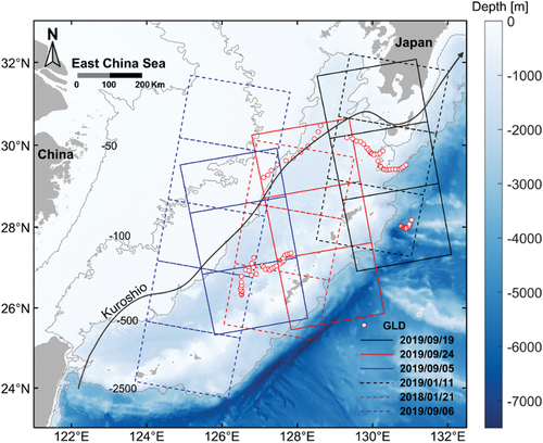
0.7–0.8 km) (Biron, Van Wychen, and Vachon Citation2018). The IW mode consisted of three sub-swaths (IW1, IW2, and IW3) with incidence angles from near to far between 30°to-36°, 36°to-42°, and 41°to-46°, respectively. shows the spatial locations of the adopted nine ascending scenes (2019/09/19, 2019/09/24, and 2019/09/05) and 11 descending scenes (2019/01/11, 2018/01/21, and 2019/09/06).
Figure 1. Bathymetric map of the Kuroshio region. The solid and dashed lines represent the ascending and descending SAR data passes, respectively, the red circles are GLD buoy data, and the download link for bathymetry data: https://topex.ucsd.edu/pub/srtm15_plus/.
2.2. Validation datasets
The validation datasets included Global Surface Lagrangian Drifter (GLD) data, Global Ocean Multi-observation products (MOB), and Regional Ocean Circulation Model (ROMS) numerical simulation currents. GLD data were provided by the Drifter Data Assembly Center at NOAA (Atlantic Oceanographic and Meteorological Laboratory, https://www.aoml.noaa.gov/envids/). The ocean surface current velocity is calculated from the position changes captured by buoys, and then optimally interpolated to uniform 6-hour resolution (Krug et al. Citation2010; Wang et al. Citation2021). To compare with the SAR radial current velocity, GLD data recorded during 48 h were collected and projected onto the SAR range direction. A total of 67 points in the ascending scene and 27 points in the descending scene were used to validate SAR velocities.
MOB product (http://marine.copernicus.eu) belongs to global total ocean current reanalysis data with a 1 h frequency and a one-fourth deg regular grid, and the product ID is MULTIOBS_GLO_PHY_MYNRT_015_003. The total current fields consist of geostrophic and Ekman currents at the surface and 15 m depth, obtained by combining CMEMS satellite-observed geostrophic surface currents with Ekman currents simulated using ERA5 wind stress. Compared with MOB product, model currents have higher spatial resolution. The numerical simulation of the ocean surface current was based on a high-resolution 3D model established by the ROMS model. It employed terrain-following coordinates in the vertical direction with 15 layers and a grid spacing of 1.5 km. The model adopts the Bulk Formula method for atmospheric forcing, with upper boundary condition derived from the National Centers for Environmental Prediction (NCEP) data at 6-hour intervals. Vertical mixing and tidal forcing were implemented using universal length-scale turbulence mixing and the TPXO9 dataset. The initial conditions and open boundary conditions for the model have been derived from HYCOM hydrographic dataset (spatial resolution of 0.08° × 0.08°) (Jang et al. Citation2021). Finally, the temporal and spatial resolutions of the output data are 0.5 h and 1.5 km, respectively.
These datasets are potentially different due to differences in sources. GLD data have the highest accuracy, but the coverage and quantity are limited. MOB product can effectively show the direction of strong ocean currents, but the spatial resolution is low, suitable only for displaying the direction of the Kuroshio central current. Compared with reanalysis data, ROMS model currents enhance the spatiotemporal resolution of simulated flows by employing higher-resolution grids and time steps, serving as an effective supplement to GLD and MOB data.
3. Methodology
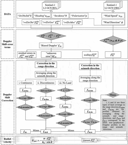
3.1. Doppler shift caused by currents
For Sentinel-1 OCN data, the total observed Doppler shift () includes geophysical and non-geophysical components (EquationEquation (1)
(1)
(1) ).
where is the geophysical term induced by wind-wave
and current
(EquationEquation (2)
(2)
(2) ) (Moiseev, Johannessen, and Johnsen Citation2022). From EquationEquation (3)
(3)
(3) ,
is the non-geophysical term, groups the geometrical term
, the antenna miss-pointing term
, the scalloping
and unknown error term
. Among these,
is generated by the satellite velocity relative to the rotating earth, and
is due to the deviation between the actual antenna pattern and the theoretical antenna pattern, which can be regarded as a function of the incidence angle.
occurs due to the antenna gain variation, and
is due to the sensor temperature compensation and inaccurate estimation of the non-geophysical Doppler shifts.
The initial calibrations for and
are based on the variables (“rvlDcGeo” and “rvlDcMiss”) provided by the Sentinel-1 Level 2 OCN product. However, these two computed terms are imprecise (Johnsen et al. Citation2016). There are noticeable residual non-geophysical biases, as scalloping and the land signals are not equal to 0 Hz (Danilo and Bella Citation2018). The residual errors mentioned above, together with
and
are defined as
in this study. As these errors,
appears linear variation with incidence angle in the radial or range direction and jumps over sub-swaths. This is related to the antenna miss-pointing, and this “range bias” usually requires subtracting the average Doppler shift over land. In addition,
presents a scallop effect with significant periodic changes (±10 Hz) along the azimuth direction. This is an artifact that hinders the direct analysis of the spatial changes of surface current velocity (Wang et al. Citation2023). Therefore,
can be decomposed into two radar directions for correction: the range and the azimuth direction (see 3.2 for more details). The geophysical Doppler
is obtained after subtracting
. In order to retrieve ocean surface current
from
, the empirical geophysical model function (GMF) called CDOP is used to estimate and remove the wind-wave bias
(see EquationEquation (4)
(4)
(4) ) (Elyouncha, Eriksson, and Johnsen Citation2022; Moiseev et al. Citation2020). The input parameters of the CDOP model include wind speed (
) and direction (
) at 10 m height retrieved from SAR images provided in Sentinel-1 Level 2 OWI products (“owiWindSpeed” and “owiWindDirection”), incidence angle (
) and polarization (
) at C-band SAR. The Doppler shift contributed by the ocean current can be expressed as:
The SAR radial surface velocity can be derived from the estimated as EquationEquation (5)
(5)
(5) ,
where is the electromagnetic wave number for Sentinel-1, which is equal to 113.28 m−1, and
is the incidence angle. The overall workflow () of radial velocity inversion includes range and azimuth calibrations.
Figure 2. The flowchart of the data processing.
3.2. Non-geophysical Doppler shift correction algorithm
3.2.1. Correction in the range direction
The biased Doppler shift fails to correctly represent the non-geophysical parameters variations along the range direction, especially as observed over land. Based on the assumption that the Doppler shift over land should be 0 Hz, the residual deviation can be approximated by the averaged Doppler shift in data over land (Wang et al. Citation2022). However, there are three types of land coverage in the range direction according to the “rvlLandCoverage” variable from Sentinel-1 OCN data: (1) continuous land coverage, (2) non-continuous land coverage, and (3) no land coverage. We proposed three corresponding schemes.
Scheme i, the method applies to continuous land in the range direction, as seen the IW3 in of the SAR image from 19 September 2019. An algorithm combining average filtering and polynomial fitting (AP) was proposed. Specifically, the mean range profile was first obtained by averaging the Doppler shifts over land along the azimuth direction (EquationEquation (6)
(6)
(6) ). From EquationEquation (7)
(7)
(7) , the
is smoothed by an average filter to reduce the interference of abrupt signals, followed by polynomial fitting to obtain the range profile
. The calibration of range bias is achieved by subtracting
from
.
Figure 3. Three correction schemes in the range direction.
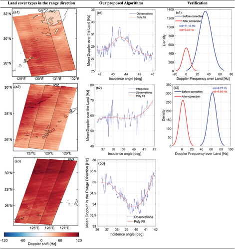
where and
denote the azimuth and range indices of Doppler shift grid, which are equal to the rows and columns in 2D matrix, respectively.
is the component in the range direction in set
.
and
are 1D digital average filter and polynomial fit functions. The results of
and
correspond to the blue and red lines in ), respectively.
Scheme ii, a method for the discontinuous land in the range direction, such as IW3 in 2) from 21 January 2018. Using EquationEquation (6)(6)
(6) fails to produce a continuous
. To avoid the strong discontinuities in the calibration results, we combine an interpolation method with Scheme i (called IAP). Specifically, using a moving window to interpolate the missing values in
with the median value in the neighborhood. As for the SAR image in , the window size of 19, and the interpolated profile is denoted by a dotted line in . Then, using EquationEquation (7)
(7)
(7) to compute
, and subtract it from
to perform range bias calibration.
Scheme iii, a method named NIAP for the no land in SAR image or reference image (adjacent orbit and same period). As seen the IW1 in of from 6 September 2019, neither scheme i or ii is applicable. This limits the application of SAR data to monitor ocean currents without land coverage. If the Normalized Radar Cross Section (NRCS) variations of the SAR data are not significant (i.e. non-complex sea conditions), we propose exploiting the Doppler shift over the ocean to simulate non-geophysical Doppler shift variations, following the linear variation in the range direction (Wang et al. Citation2022; Yang and Yijun Citation2023). However, it is worth noting that the Doppler shifts over the land are often smaller than in the ocean due to the sea surface motion. Therefore, the empirical conditions adopted by Danilo and Bella (Citation2018) was introduced to calculate . According to the “rvlDcObsStd” variable in Sentinel-1 Level 2 OCN products, the outliers or high-frequency values with a standard deviation exceeding 4 Hz were first removed. Then,
is obtained by averaging along the azimuthal direction, and we also set the minimum sample for computing the profile to 10 pixels to reduce the interference from the abrupt signal. Additionally, it is necessary to apply interpolation consistent with Scheme ii to ensure
is continuous. Finally,
is obtained by EquationEquation (7)
(7)
(7) , and subtracted from
to calibrate the range bias.
The above correction method in the range direction can be expressed by the following pseudocode:
Table
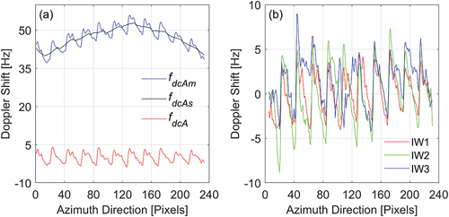
3.2.2. Correction in the azimuth direction
There still exists 10 Hz periodic variation along the azimuth direction in the SAR image after range bias calibration. To remove the scalloping, we define the Doppler shift after range calibration as
. We aim to identify the burst period of the scalloping by calculating
,
and
. Specifically,
is the mean azimuth profile obtained by averaging along the range direction in each sub-swath data, and an average filter smoothing is applied to
to get
. The period variation signal
then is obtained by subtracting
from
. In ,we select one of the SAR images in to show the azimuth calibration process. shows IW1 of the selected data, and the blue, black, and red lines correspond to
,
and
, respectively. The
in IW2 and IW3 are also obtained through this method (). Finally,
is subtracted from
to complete the azimuth calibration.
Figure 4. Doppler shifts in the azimuth direction, with is a 10 Hz periodic variation. Figure (a) shows the identification process of the scalloping (only IW1 swath), while figure (b) shows the method applied to the full image.
4. Results
4.1. Kuroshio retrieval
As shown in , the is positive when the ocean surface current moves away from the radar sensor, while negative velocity is toward the radar sensor (Van Wychen et al. Citation2018). The Appendix contains the results of current inversions of SAR data for other time phases. The velocity of the central Kuroshio is between 0.5 and 1 m/s and meanders along the Okinawa Trough from southwest to northeast.
Figure 5. Result of current retrieval. Figures (a) and (b) show the radial velocities on September 24, 2019, and January 21, 2018, respectively. The Kuroshio central current is the blue line, and the Kuroshio counter Current is the red line. The arrows are derived from the MOB products.
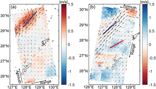
corresponds to red in , indicating the Kuroshio central current at (28°N-30°N) meanders northeastward along the Ryukyu Trench with a width of 40–60 km. At 28.5°–30.5° N, 127.5°–130° E, the velocity in the Kuroshio central current region is significantly higher than in the neighborhoods, forming a straight and fast-flowing current zone that bends and flows toward the adjacent sea regions, rather than a single flow direction.
corresponds to red in and clearly shows the characteristics of the Kuroshio central current, but the width is narrower, between 20 and 30 Km. Additionally, the Kuroshio Counter Current is more significant in , corresponding to the blue region with
, which is located at 26.5°–27.8°N, 127.5°E-128.5°E, and the velocities are between 0.4 and 0.6 m/s. Both SAR radial velocity and MOB products observe the Kuroshio central current (blue line) and the Kuroshio Counter Current (red line).
4.2. Comparison with GLD data
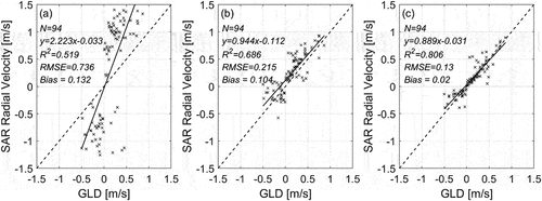
To compare with different ocean current data, the GLD data and ROMS ocean model were projected onto the SAR radial direction (Rio, Mulet, and Picot Citation2014). The statistical analysis is found by comparing the calibrated radial velocities from 6 Sentinel-1 scenes with 94 collocated GLD points. In , is only corrected the scalloping without range bias calibration, and the root mean square error (RMSE) and correlation coefficient (R2) are 0.736 m/s and 0.519, respectively. After correcting in the range direction, R2 increased from 0.519 to 0.686, while RMSE decreased from 0.736 m/s to 0.215 m/s (). After removing the wind-wave
, R2 ≈0.806 and RMSE ≈0.13 m/s (). These all passed the significance test with a P-value less than 0.001. The correlation coefficients are significant at a confidence level of 99%. Therefore, the ocean current velocities retrieved from SAR image have a reliable accuracy that can be applied to the comprehensive observation of ocean hydrodynamic parameters.
Figure 6. Comparing SAR radial surface velocity with the GLD data. Figure (a) is only the azimuth correction completed, while figure (b) shows the results of range and azimuth calibration. Figure (c) shows the results of wind-wave bias correction.
4.3. Comparison with ocean model
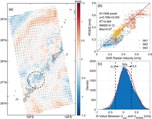
shows the ocean current provided by the ROMS model on 24 September 2019, with 1.5 km × 1.5 km. This is generally consistent with the SAR inversion, but there are also local differences, especially in the coastal regions (black circles). There is a coastal current from northeast to southwest at approximately −0.3 to −0.5 m/s, but this was not detected by SAR in . We infer that this is related to the interference of land signals in SAR images. There is a significant change in the gradient of the land echo signal along the coastal and land boundaries. Current research usually masks a distance range (approximately 10 km) along the coast (Moiseev, Johannessen, and Johnsen Citation2022; Wang et al. Citation2021). For statistical analysis, we randomly selected 1949 points within the Kuroshio Current of each swath. shows an R2 of 0.664 and RMSE of 0.12 m/s, while demonstrates that approximately 70% of the values fall within the range of −0.3 to 0.3 m/s. The visualizations of the two types of ocean current data are generally consistent, but the retrieved velocity is typically higher than the velocity provided by the ROMS model. This is related to disparity in data sources. The spatial resolution of the reanalysis data selected for the initial field of the ROMS model is low, and the grid is rough. This may result in an underestimation of the velocity in some regions.
Figure 7. Comparison with ROMS model. (a) shows the ROMS model projected onto the SAR radial direction. (b) depicts a scatter, with different colors representing matching points from different swaths. (c) shows the histogram of the velocities difference (D-Value) between SAR and ROMS.
5. Discussion
5.1. Influence of proposed non-geophysical corrections
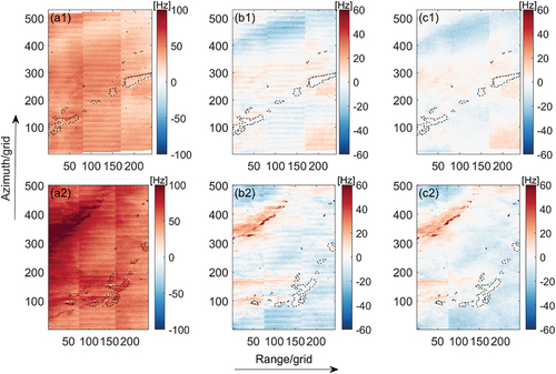
In , we take two SAR scenes in on 24 September 2019, and 21 January 2018, as examples to show the changes before and after non-Doppler shift correction. From , it is difficult to directly observe the features of the ocean currents due to the non-geophysical Doppler effect, such as Doppler shifts over land are not equal to 0 Hz and scalloping. The empirical strategies were proposed to reduce the impact of non-geophysical parameters on ocean current observations. The mean value of Doppler shifts over land after bias correction close to 0 Hz after range bias calibration (see , and this satisfies the “zero motion” assumption. However, the significant scallop signals can still be observed in the azimuth direction. From , it is found that the correction method in Section 5.2.1 is suitable for scalloping calibration and improving the quality of Sentinel-1 OCN data. We subsequently proceed to assess the effectiveness of the proposed calibration scheme.
Figure 8. Non-geophysical Doppler correction. (a1) and (a2) show the biased Doppler shift . (b1) and (b2) show the results after correction in the range direction. (c1) and (c2) show the effective geophysical Doppler shift
after removing the scalloping.
The first significant artifact is that the Doppler shift over land is not equal to 0 Hz, which is related to inaccurate estimation of and
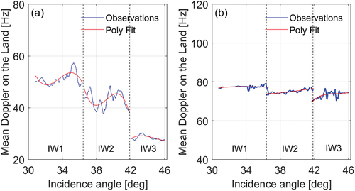
. A common solution is averaging over land to estimate the range bias. For scenes with land, Schemes i and ii in Section 3.2.2 can be selected to correct the absolute bias. In , both ascending () and descending () passes exhibit similar variations in the range direction. From IW1 to IW3, the range bias shows a linear downward as the incidence angles increase and jump over swaths. The values of IW1 are higher than the other two swaths, so the impact of non-geophysical bias is more significant in the near range direction. The results indicate that the range bias can be approximated as a function of the incidence angle.
Figure 9. Non-geophysical Doppler shift variation in range direction. Figures (a) and (b) show the estimated range bias for the ascending (19 September 2019) and descending (11 January 2019), respectively. Blue line is the mean Doppler shift over land along azimuth, and red line is the error fitting value.
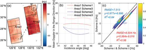
For scenes without land, it is possible to estimate by interpolating from reference images with the adjacent orbits and the same period. However, there are some extreme phenomena without appropriate reference data in the open sea. Therefore, Scheme iii in Section 3.2.2 attempts to use data over the ocean under non-complex sea conditions. From , Area 1 and Area 2 are selected to compare different range bias correction schemes. For Area 1, we compared Scheme i and iii, and the red lines in show the range bias fitting of the two methods, with a mean deviation of about 8 Hz. The blue lines in display the range bias fitting of Scheme i and 3 in Area 2, with a mean deviation of about 6 Hz. In summary, the error between Scheme iii and Scheme i or ii is within one scalloping period. The statistical analysis in reveals the correlation of range calibration results between Scheme iii and Scheme i, as well as between Scheme iii and Scheme ii, and R2 equal to 0.84 and 0.98, respectively. Therefore, in the absence of a land reference image, if the variations in NRCS are not significant, that is non-complex sea conditions such as typhoons, strong tidal currents, and eddies. Scheme iii is suitable for range error correction without land coverage.
Figure 10. Comparison of three range bias estimation schemes.
5.2. Sensitivity analysis for SAR current results
5.2.1. Influence of SAR geometry parameters
The satellite track and incidence angles are the two important geometric parameters that impact the quality of radial velocity retrieval. The Sentinel-1 track angle of ascending and descending passes are ∼350° and ∼190° (clockwise rotation from the north), respectively. In the study area, these passes are, respectively, aligned with the offshore (from land to sea) and onshore (from sea to land) wind direction, as well as correspond to the direction of Kuroshio (southwest-northeast) and Kuroshio Counter Current (northeast-southwest). When the wind-wave is propagating near the satellite track or azimuth direction, the impact on gathering Doppler signals collected in the range direction will be lessened, and this is more significant in high incidence angle. Therefore, in the ascending pass on 24 September 2019, the observed trajectory of the Kuroshio central current reveals a higher degree of overlap with GLD buoy data in the same region compared to the descending pass. We conclude that ascending passes are more suitable for monitoring and mapping ocean currents for the Kuroshio.
Both radar backscatter and Doppler shift estimations from wind/waves are affected by the incidence angle. The lower incidence angle receives stronger echo signals. This implies that low incidence angles are more sensitive to high flow velocity and rough ocean surfaces and thus have a greater impact on ocean current inversion accuracy. Based on the collected Sentinel-1 SAR images, we found that the observed Doppler shifts in IW1 are usually higher than those in IW2 and IW3, and the error of was correspondingly more significant. When the land coverage is discontinuous, SAR images with land coverage at neighboring orbits and times can be used as a reference and combined with moving average and polynomial fitting for error estimation. When there is no land coverage, the Doppler shift in the range direction can be estimated by interpolating the neighboring values in the neighborhood; however, this scheme is not optimal and is only applicable to calm ocean conditions. Therefore, schemes ii and iii in this study may be prone to overestimating the error in the range direction, as observed in IW1. The incidence angle increases from 30° to 46° when compared to GLD data, and the RMSE is 0.16 m/s, 0.12 m/s, and 0.11 m/s, respectively. Furthermore, the agreement of velocity with GLD and ROMS was better in IW2 and IW3 than in IW1, with IW3 showing the best effect. In general, applying our suggested methods to remove non-geophysical components can reveal the underlying geophysical signatures and improve the quality of the data.
5.2.2. Influence of wind-wave bias on RVL
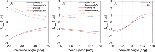
The SAR radial surface velocity (RVL, also called Doppler velocity) generated by wind/wave can be estimated and eliminated by CDOP model (Elyouncha, Eriksson, and Johnsen Citation2022). To distinguish between the RVL generated by wind/wave and current, we define the former as , which is related to radar parameters (incidence angle and polarization) and ocean conditions (wind speed and direction), as shown in .
For the C-band SAR data, in the HH polarization is higher than that in the VV polarization, making it more sensitive to signals produced by the wind wave. In ,
reduces as the incidence angle increases when the wind speed
, and the relative wind direction
, indicating the influence of wind and waves on the ocean current is lessened and the accuracy of radial velocity retrieval is improved. In , when the incidence angle
and relative wind direction
,
increases with the wind speed, showing that there is a more significant effect of wind/wave on current at high wind speed. shows
variation with relative wind direction for incidence angle
and wind speed
, and
is not symmetrical to the wind direction.
is greater in upwind (
) than in downwind (
), while
in the crosswind. Therefore, the influence of wind/wave bias is more significant in the upwind than in the downwind and crosswind (
). However, assessment of the contribution of the sea state to the geophysical Doppler shift remains a challenging task (Kudryavtsev et al. Citation2023). In the future, we will consider the influence of wave parameters such as ocean significant wave height, peak frequency, and direction under complex ocean conditions (Yurovsky et al. Citation2019).
Figure 11. Variation of the Doppler velocity contributed by the ocean condition for different incidence angles, wind speeds, wind directions, and polarization parameters.
6. Conclusion
In this study, we developed a non-geophysical Doppler shifts correction algorithm. The advantage of the algorithm lies in resolving the absence of land coverage for range bias calibration, when using Sentinel-1 IW mode SAR to monitor Kuroshio. In addition, we compared and analyzed the SAR current inversion with the ocean current derived from Global Surface Lagrangian Drifter (GLD) and Regional Ocean Circulation Model (ROMS).
The proposed algorithm includes two steps: range and azimuth direction correction. In the range direction, we considered various land coverages and proposed three schemes (AP, IAP, and NIAP) to minimize residual antenna miss-pointing and unknown error. The core of the schemes includes average filter, polynomial fit, and interpolation. The 1D digital average filtering is also used to eliminate the scalloping in the azimuth direction. The non-geophysical Doppler shifts in these two directions are theoretically independent; therefore, the two steps can be exchanged when processing the data. The non-geophysical Doppler shifts correction algorithm can significantly improve the Sentinel-1 OCN data, resulting in a higher quality of Kuroshio observation and mapping.
The analysis of the SAR current inversion shows that the velocity of the central Kuroshio is between 0.5 and 1 m/s. The ascending and descending passes are suitable for the observation of Kuroshio central current and Kuroshio counter current, respectively. After non-geophysical and wind-wave Doppler calibration, the R2 between SAR radial velocity and GLD range velocity are 0.686 and 0.806, with RMSE of 0.215 and 0.13, respectively. Furthermore, there was good agreement between the SAR current inversion and the ROMS ocean model. The regions where the Kuroshio flows are mainly situated in the open sea, lacking HF radar, gliders, and other observation. This limitation hinders further studies to conduct more statistical and comparative analyses. Nevertheless, the non-geophysical Doppler shift calibration performed in the case of Kuroshio demonstrates the feasibility and robustness of the method. In subsequent research, we will apply the method to the Gulf Stream and conduct a more systematic analysis with the collected public HF Radar data.
At present, wind-wave bias estimation and 2D ocean surface current vector inversion are still two major challenges in providing the reliable current fields by SAR Doppler shift. If we can obtain more satellite or in-situ observation data, these can be used to analyze the contribution of nonlinear hydrodynamic factors to ocean currents, and enhance the practicality of the method under complex ocean conditions. In addition, the current vector might be attempted by combining the Doppler Centroid Anomaly (DCA) method with sub-aperture decomposition. In conclusion, Sentinel-1 IW mode SAR data hold great potential in ocean current mapping. This study serves as an effective complement to non-geophysical Doppler calibration and provides support for the construction of ocean current time series data sets, making it crucial for remote sensing observations in ocean dynamics.
SupplementaryClean.docx
Download MS Word (1.5 MB)Acknowledgments
The authors sincerely thank the ESA for providing Sentinel-1 SAR products and all anonymous reviewers who provided detailed and valuable comments or suggestions to improve this manuscript.
Disclosure statement
The authors declare that they have no known competing financial interests or personal relationships that could have appeared to influence the work reported in this paper.
Data availability statement
The Sentinel-1 SAR OCN products that support the findings of this study are openly available at https://scihub.copernicus.eu/dhus/#/home.
Supplementary material
Supplemental data for this article can be accessed online at https://doi.org/10.1080/15481603.2024.2304956.
Additional information
Funding
References
- Bellomo, L., A. Griffa, S. Cosoli, P. Falco, R. Gerin, I. Iermano, A. Kalampokis, et al. 2015. “Toward an Integrated HF Radar Network in the Mediterranean Sea to Improve Search and Rescue and Oil Spill Response: The TOSCA Project Experience.” Journal of Operational Oceanography 8 (2): 95–16. https://doi.org/10.1080/1755876X.2015.1087184.
- Biron, K., W. Van Wychen, and P. W. Vachon. 2018. “Gulf Stream Detection from SAR Doppler Anomaly.” Canadian Journal of Remote Sensing 44 (4): 311–320. https://doi.org/10.1080/07038992.2018.1516130.
- Chapron, B., F. Collard, and F. Ardhuin. 2005. “Direct Measurements of Ocean Surface Velocity from Space: Interpretation and Validation.” Journal of Geophysical Research Oceans 110 (C7). https://doi.org/10.1029/2004JC002809.
- Danilo, C., and G. Bella. 2018. “Extracting Usable Geophysical Doppler Properties from Sentinel–1 for Coastal Monitoring.” Paper presented at the 2018 Doppler Oceanography from Space (DOfS), Oct 10-12.
- Elyouncha, A., L. E. B. Eriksson, and H. Johnsen. 2022. “Direct Comparison of Sea Surface Velocity Estimated from Sentinel-1 and TanDEM-X SAR Data.” IEEE Journal of Selected Topics in Applied Earth Observations & Remote Sensing 15:2425–2436. https://doi.org/10.1109/JSTARS.2022.3158190.
- Elyouncha, A., L. E. B. Eriksson, H. Johnsen, and L. M. H. Ulander. 2019. “Using Sentinel-1 Ocean Data for Mapping Sea Surface Currents Along the Southern Norwegian Coast.” Paper presented at the IGARSS 2019 - 2019 IEEE International Geoscience and Remote Sensing Symposium, 28 July-2 August. 2019, Yokohama, Japan.
- Ferreira, R. M., S. F. Estefen, and R. Romeiser. 2016. “Under What Conditions SAR Along-Track Interferometry is Suitable for Assessment of Tidal Energy Resource.” IEEE Journal of Selected Topics in Applied Earth Observations & Remote Sensing 9 (11): 5011–5022. https://doi.org/10.1109/JSTARS.2016.2581188.
- Gens, R. 2008. “Oceanographic Applications of SAR Remote Sensing.” GIScience & Remote Sensing 45 (3): 275–305. https://doi.org/10.2747/1548-1603.45.3.275.
- Hansen, M. W., F. Collard, K. F. Dagestad, J. A. Johannessen, P. Fabry, and B. Chapron. 2011. “Retrieval of Sea Surface Range Velocities from Envisat ASAR Doppler Centroid Measurements.” IEEE Transactions on Geoscience & Remote Sensing 49 (10): 3582–3592. https://doi.org/10.1109/TGRS.2011.2153864.
- Hansen, M. W., V. Kudryavtsev, B. Chapron, J. A. Johannessen, F. Collard, K. F. Dagestad, and A. A. Mouche. 2012. “Simulation of Radar Backscatter and Doppler Shifts of Wave–Current Interaction in the Presence of Strong Tidal Current.” Remote Sensing of Environment 120:113–122. https://doi.org/10.1016/j.rse.2011.10.033.
- Huaming, Y., L. Jiangyu, W. Kejian, Z. Wang, Y. Haiqing, S. Zhang, Y. Hou, and R. M. Kelly. 2018. “A Global High-Resolution Ocean Wave Model Improved by Assimilating the Satellite Altimeter Significant Wave Height.” International Journal of Applied Earth Observation and Geoinformation 70: 43–50. https://doi.org/10.1016/j.jag.2018.03.012.
- Jang, E., Y. Jun Kim, I. Jungho, and Y.-G. Park. 2021. “Improvement of SMAP Sea Surface Salinity in River-Dominated Oceans Using Machine Learning Approaches.” GIScience & Remote Sensing 58 (1): 138–160. https://doi.org/10.1080/15481603.2021.1872228.
- Johannessen, J. A., B. Chapron, F. Collard, V. Kudryavtsev, A. Mouche, D. Akimov, and K. F. Dagestad. 2008. “Direct Ocean Surface Velocity Measurements from Space: Improved Quantitative Interpretation of Envisat ASAR Observations”. Geophysical Research Letters 35(22). https://doi.org/10.1029/2008GL035709.
- Johannessen, J. A., R. P. Raj, J. E. Ø Nilsen, T. Pripp, P. Knudsen, F. Counillon, D. Stammer, et al. 2014. “Toward Improved Estimation of the Dynamic Topography and Ocean Circulation in the High Latitude and Arctic Ocean: The Importance of GOCE.” Surveys in Geophysics 35 (3): 661–679. https://doi.org/10.1007/s10712-013-9270-y.
- Johnsen, H., V. Nilsen, G. Engen, A. A. Mouche, and F. Collard. 2016. “Ocean Doppler Anomaly and Ocean Surface Current from Sentinel 1 Tops Mode.” Paper presented at the 2016 IEEE International Geoscience and Remote Sensing Symposium (IGARSS), July 10-15.
- Kravtsov, Y. A., A. V. Kuz’min, O. Yu Zavrova, L. M. Mitnik, M. I. Mityagina, K. D. Sabinin, and Y. G. Trokhimovskiy. 1998. “Polarization features of radar images of internal waves on the ocean surface.” Mapping Sciences and Remote Sensing 35 (3): 173–186. https://doi.org/10.1080/07493878.1998.10642089.
- Krug, M., A. Mouche, F. Collard, J. A. Johannessen, and B. Chapron. 2010. “Mapping the Agulhas Current from Space: An Assessment of ASAR Surface Current Velocities.” Journal of Geophysical Research Oceans 115 (C10. https://doi.org/10.1029/2009JC006050.
- Kudryavtsev, V., D. Akimov, J. Johannessen, and B. Chapron. 2005. “On Radar Imaging of Current Features: 1. Model and Comparison with Observations.” Journal of Geophysical Research Oceans 110 (C7). https://doi.org/10.1029/2004JC002505.
- Kudryavtsev, V., S. Fan, B. Zhang, B. Chapron, J. A. Johannessen, and A. Moiseev. 2023. “On the Use of Dual Co-Polarized Radar Data to Derive a Sea Surface Doppler Model—Part 1: Approach.” IEEE Transactions on Geoscience & Remote Sensing 61:1–13. https://doi.org/10.1109/TGRS.2023.3235829.
- Martin, A. C. H., C. P. Gommenginger, B. Jacob, and J. Staneva. 2022. “First Multi-Year Assessment of Sentinel-1 Radial Velocity Products Using HF Radar Currents in a Coastal Environment.” Remote Sensing of Environment 268:112758. https://doi.org/10.1016/j.rse.2021.112758.
- Melet, A., P. Teatini, G. Le Cozannet, C. Jamet, A. Conversi, J. Benveniste, and R. Almar. 2020. “Earth Observations for Monitoring Marine Coastal Hazards and Their Drivers.” Surveys in Geophysics 41 (6): 1489–1534. https://doi.org/10.1007/s10712-020-09594-5.
- Moiseev, A., J. A. Johannessen, and H. Johnsen. 2022. “Towards Retrieving Reliable Ocean Surface Currents in the Coastal Zone from the Sentinel-1 Doppler Shift Observations.” Journal of Geophysical Research Oceans 127 (5): e2021JC018201. https://doi.org/10.1029/2021JC018201.
- Moiseev, A., H. Johnsen, J. A. Johannessen, F. Collard, and G. Guitton. 2020. “On Removal of Sea State Contribution to Sentinel-1 Doppler Shift for Retrieving Reliable Ocean Surface Current.” Journal of Geophysical Research Oceans 125 (9): e2020JC016288. https://doi.org/10.1029/2020JC016288.
- Mouche, A. A., F. Collard, B. Chapron, K. F. Dagestad, G. Guitton, J. A. Johannessen, V. Kerbaol, and M. W. Hansen. 2012. “On the Use of Doppler Shift for Sea Surface Wind Retrieval from SAR.” IEEE Transactions on Geoscience & Remote Sensing 50 (7): 2901–2909. https://doi.org/10.1109/TGRS.2011.2174998.
- Paduan, J. D., and L. Washburn. 2013. “High-Frequency Radar Observations of Ocean Surface Currents.” Annual Review of Marine Science 5 (1): 115–136. https://doi.org/10.1146/annurev-marine-121211-172315.
- Rascle, N., B. Chapron, J. Molemaker, F. Nouguier, J. O.-T. Francisco, J. Pedro Osuna Cañedo, L. Marié, B. Lund, and J. Horstmann. 2020. “Monitoring Intense Oceanic Fronts Using Sea Surface Roughness: Satellite, Airplane, and in situ Comparison.” Journal of Geophysical Research Oceans 125 (8): e2019JC015704. https://doi.org/10.1029/2019JC015704.
- Rashid, M., and C. H. Gierull. 2021. “Retrieval of Ocean Surface Radial Velocities with RADARSAT-2 Along-Track Interferometry.” IEEE Journal of Selected Topics in Applied Earth Observations & Remote Sensing 14:9597–9608. https://doi.org/10.1109/JSTARS.2021.3110198.
- Rio, M. H., S. Mulet, and N. Picot. 2014. “Beyond GOCE for the Ocean Circulation Estimate: Synergetic Use of Altimetry, Gravimetry, and in situ Data Provides New Insight into Geostrophic and Ekman Currents.” Geophysical Research Letters 41 (24): 8918–8925. https://doi.org/10.1002/2014GL061773.
- Röhrs, J., G. Sutherland, G. Jeans, M. Bedington, A. Kristin Sperrevik, K.-F. Dagestad, Y. Gusdal, C. Mauritzen, A. Dale, and J. H. LaCasce. 2021. “Surface Currents in Operational Oceanography: Key Applications, Mechanisms, and Methods.” Journal of Operational Oceanography 16 (1): 60–88. https://doi.org/10.1080/1755876X.2021.1903221.
- Shen, Y.-T., J.-W. Lai, L.-G. Leu, L. Yi-Chieh, J.-M. Chen, H.-J. Shao, H.-W. Chen, et al. 2019. “Applications of Ocean Currents Data from High-Frequency Radars and Current Profilers to Search and Rescue Missions Around Taiwan.” Journal of Operational Oceanography 12 (sup2): S126–S136. https://doi.org/10.1080/1755876X.2018.1541538.
- Sun, K., J. Chong, L. Diao, Z. Li, and X. Wei. 2022. “On the Use of Ocean Surface Doppler Velocity for Oceanic Front Extraction from Chinese Gaofen-3 SAR Data.” IEEE Journal of Selected Topics in Applied Earth Observations & Remote Sensing 15:2709–2720. https://doi.org/10.1109/JSTARS.2022.3162445.
- Van Wychen, W., P. W. Vachon, J. Wolfe, and K. Biron. 2018. “The Utility of Sentinel-1 Data for Ocean Surface Feature Analysis in the Vicinity of the Gulf Stream.” Canadian Journal of Remote Sensing 44 (2): 144–152. https://doi.org/10.1080/07038992.2018.1461558.
- Wang, L., Y. Gao, L. Peng, L. Fan, and Y. Zhou. 2022. “A New Doppler Frequency Anomaly Algorithm for Surface Current Measurement with SAR.” Journal of Oceanology and Limnology 40 (2): 470–484. https://doi.org/10.1007/s00343-021-0492-4.
- Wang, L., B. Shi, Y. Zhou, H. Sheng, Y. Gao, L. Fan, and Z. Yang. 2021. “Radial Velocity of Ocean Surface Current Estimated from SAR Doppler Frequency Measurements—A Case Study of Kuroshio in the East China Sea.” Acta Oceanologica Sinica 40 (12): 135–147. https://doi.org/10.1007/s13131-021-1883-2.
- Wang, R., W. Zhu, X. Zhang, Y. Zhang, and J. Zhu. 2023. “Comparison of Doppler-Derived Sea Ice Radial Surface Velocity Measurement Methods from Sentinel-1A IW Data.” IEEE Journal of Selected Topics in Applied Earth Observations & Remote Sensing 16:2178–2191. https://doi.org/10.1109/JSTARS.2023.3241978.
- Yang, X., and H. Yijun. 2023. “Retrieval of a Real-Time Sea Surface Vector Field from SAR Doppler Centroid: 2. On the Radial Velocity.” Journal of Geophysical Research Oceans 128 (1): e2022JC019301. https://doi.org/10.1029/2022JC019301.
- Yoshida, T., K. Ouchi, and C. S. Yang. 2021. “Application of MA-ATI SAR for Estimating the Direction of Moving Water Surface Currents in Pi-SAR2 Images.” IEEE Journal of Selected Topics in Applied Earth Observations & Remote Sensing 14:2724–2730. https://doi.org/10.1109/JSTARS.2021.3060008.
- Yurovsky, Y. Y., V. N. Kudryavtsev, S. A. Grodsky, and B. Chapron. 2019. “Sea Surface Ka-Band Doppler Measurements: Analysis and Model Development.” Remote Sensing 11 (7): 839. https://doi.org/10.3390/rs11070839.