A novel landslide susceptibility prediction framework based on contrastive loss

ABSTRACT

Recently, the positive unlabeled (PU) learning algorithms have proven highly effective in generating accurate landslide susceptibility maps. The algorithms categorize samples exclusively into positive samples (landslides) and unlabeled samples for training, eliminating random or subjective selection of non-landslide samples. However, existing PU learning algorithms face limitations in capturing correct negative samples in multi-genesis landslide areas, leading to lower prediction accuracy. To address this issue, the PU-pullbaggingDT algorithm was proposed in this study. This integrated method combines the strengths of two techniques: the superior ranking performance of the PU-baggingDT algorithm and the low bias of the contrastive learning approach. The contrastive learning introduces a new contrastive loss of PU learning (PUpull loss), which pulls the distance of similar landslide samples in the projection space closer based on the validation accuracy threshold, without the need for data augmentation and class probability. The PUpull loss relaxes the tightness toward unlabeled samples, reducing the impact of incorrectly defined non-landslide samples on prediction results in multi-genesis landslide areas. The proposed algorithm outperforms existing PU-learning and machine learning methods (support vector machine, decision tree, logistic regression, AdaBoost, and XGBoost) with random selection of negative samples for predicting landslide susceptibility in China’s Zigui County, as demonstrated by comprehensive evaluation metrics. The landslide susceptibility mapping utilizes equal interval division and ranking, achieving approximately a 90% landslide percentage in areas with very high and high susceptibility in Zigui County. This demonstrates the capability of the proposed algorithm to effectively predict landslide susceptibility in complex geological settings.

KEYWORDS:

• Landslide susceptibility prediction
• contrastive loss
• positive unlabeled learning
• remote sensing

1. Introduction

Landslides are among the most impactful geological disasters worldwide. Landslide susceptibility mapping (LSM) is crucial for effective management, prevention, land use planning, and precise disaster prevention and reduction efforts (Aleotti and Chowdhury 1999). In the past, traditional methods, such as expert scoring, analytic hierarchy process (AHP) (Lyu, Shuilong Shen, and Arulrajah 2018), and the frequency ratio method (Langping et al. 2017) were commonly used for landslide susceptibility assessment. These methods often subjectively classify factors or define factor importance, excessively relying on subjective judgment and expert experience. However, owing to the high-dimensional data processing capability of machine learning, many scholars have begun to explore machine learning methods to assist in these assessments and reduce subjective bias. These methods include deep belief network (DBN) (W. W. Wang et al. 2020), support vector machine (SVM) (Y. Y. Huang and Zhao 2018), decision tree (DT) (T. Pham, Binh, and Prakash 2018), logistic regression (LR) (Budimir, Atkinson, and Lewis 2015), artificial neural network (ANN) (Pourghasemi et al. 2018) and random forest (RF) (Chen et al. 2014). With the development of deep learning, it has become evident that this technique has advantages in spatial data processing over traditional machine learning. Most experiments have shown that deep learning algorithms such as convolutional neural networks (CNNs) (Y. Wang, Fang, and Hong 2019) and recurrent neural networks (RNNs) (Mutlu et al. 2019) are superior to machine learning algorithms. And finally, ensemble learning, which combines multiple models for higher accuracy, has proven to be superior to single models. Examples of such ensemble approaches include AdaBoost (Kadavi, Lee, and Lee 2018), XGBoost (Sahin 2023), CNN-SVM, CNN-RF, and CNN-LR (Fang et al. 2020), as well as deep learning ensemble algorithms, such as RNN-CNN-LSTM (Kavzoglu, Teke, and Ozlem Yilmaz 2021) and BiLSTM-RNN (Haojie et al. 2021)

Many methods typically involve randomly or subjectively selecting negative samples from unknown landslide samples and then combining them with known landslide samples to construct landslide machine learning or deep learning networks (Sun et al. 2020; Al-Najjar Husam et al. 2021; Rong et al. 2021;F. Huang et al. 2020). However, owing to incomplete field surveys, missing survey data, and unknown future landslides, the spatial location of these randomly or subjectively selected negative samples cannot represent true locations where landslides will not occur or are less likely to occur (Fang et al. 2021; Qiao et al. 2020). Moreover, multi-factor landslides may involve a large number of interacting features, making it difficult to select negative samples. For instance, certain aspects of individual features may initially appear negative in isolation; however, when combined with other factors, they can exhibit a positive impact, and vice versa.

To address this issue, a method based on positive samples and unlabeled samples called positive-unlabeled learning (PU learning) has been proposed, which considers known samples of landslide points as positive samples and unknown samples as unlabeled samples. PU learning is applicable to the prediction of landslide susceptibility because a certain area that does not include known landslides should not be randomly defined as an area with a low probability of landslides, but rather should be defined as an area of unknown landslide occurrence, which corresponds to the unlabeled data defined in PU learning. This is different from binary classification, where it is necessary to define positive and negative samples. The PU learning method has been successfully applied to some aspects such as disease gene identification (Yang et al. 2012), drug – target interaction (Lan et al. 2016), and recommender systems (de Campos et al. 2018). The PU learning techniques as applied to landslide susceptibility prediction can be divided into two-step techniques and biased learning. The two-step technique refers to (1) selecting some negative samples from the unlabeled samples by strategy and (2) training the classifier with the selected negative samples and positive samples of landslides. Fang et al. (2021) selects the negative samples using adaptive sampling and the random forest algorithm (AdaPU-RF) (Fang et al. 2021). Yao et al. (2022) identified the negative samples using spy technique combined with deep learning network (T-DNN) (Yao et al. 2022). However, the identified samples with low probability of landslide are not always accurate and may result in poor classification results. In biased PU learning, unlabeled samples are considered negative examples with noise. In 2021, the PU-baggingDT algorithm was proposed (Bangyu et al. 2021), which repeatedly selects different negative samples from all unlabeled samples and trains the classifier by combining positive samples each time. Using the idea of bagging, the classification probability is obtained by averaging the scores of all trained classifiers, resulting in experiment results with a good ranking performance. However, a possibility exists that the unlabeled dataset is contaminated by positive samples. Mordelet and Vert (2014) has studied PU bagging and found that the accuracy decreases as the contamination level of the unlabeled data set increases (Mordelet and Vert 2014). Specifically, when there is a limited number of known positive samples and a certain proportion of positive samples come from unlabeled data, the predicted probabilities of positive samples (landslide points) may be low. In summary, existing PU learning techniques for landslide susceptibility prediction may result in poor negative sample identification or low susceptibility score for positive samples.

To address the issue of accuracy degradation caused by misclassification of negative samples, the contrastive learning network designed in this study effectively handles this problem. In comparison to the PU-baggingDT algorithm, contrastive learning can be used to mine the key features of landslide susceptibility responses by deep learning networks to construct instances that are similar to landslide points. The similar instances in all samples are close in the projection space, and the dissimilar instances are further away in the projection space, thus greatly reducing the possibility of positive samples from unlabeled samples being used as negative samples during training. In addition, previous studies on contrastive losses of PU learning have required the utilization of either data augmentation or class probability. (1) Data Augmentation: previous investigations into contrastive losses of PU learning primarily concentrated on text and image data, requiring the use of data augmentation objects to obtain semantically invariant samples in order to facilitate spatial alignment of samples of the same category. Acharya et al. (2022) proposed PUCL loss, suggesting the proximity of labeled anchors to all other labeled samples in the batch, while unlabeled anchors should be drawn toward their own augmentations (Acharya et al. 2022). However, it is difficult to obtain semantic invariance through data augmentation for landslide condition factors. (2) Class Probability: Some proposed contrastive losses of PU learning require setting a class probability for positive or negative samples. Faming et al. (2020) developed a debiased contrastive objective (DCL) (F. Huang et al. 2020) to correct for sampling biases of positive and negative samples with a pre-set class probability. However, it is difficult to set a class probability for positive or negative samples in landslide condition factors. In contrast to these losses, this study proposes a new contrastive loss of PU learning that can be used without the need for data augmentation and class probability. Therefore, the innovation points proposed in this paper are as follows:

1. To tackle the problem of subpar prediction performance resulting from the challenge of selecting suitable negative samples in areas with multi-factor landslides, this study introduces the PU-pullbaggingDT model, which integrates the good ranking performance of the PU-baggingDT algorithm with a low bias contrastive learning network, to achieve high precision and high-ranking results in landslide susceptibility analysis.

2. Comparing other contrastive losses of PU learning, a new pull contrastive loss of PU learning (PUpull) without the need for data augmentation and class probability was proposed to pull the distance of landslide-similar samples in the projection space closer, and to force the negative samples away from the positive samples. The degree of separation between positive samples and unlabeled samples is determined by a defined accuracy threshold for the validation set. This loss is more applicable to landslide data that are difficult to augment and is less susceptible to interference from incorrectly defined non-landslide samples while still accounting for the complex nature of multi-cause landslides.

2. Regional setting and materials

The study area was located in Zigui County, Yichang City, Hubei Province (Figure 1). Zigui County, situated in the transitional zone between the second and third topographical steps in China, is located near the Three Gorges Dam, one of the world’s largest hydraulic engineering projects. Consequently, landslides in Zigui County are influenced by the reservoir’s fluctuations resulting from the dam’s operations. The significant elevation differences, complex geological environment, and continuous human activities collectively contribute to making it one of the most disaster-prone areas in China. The study area was 2274 km² in total. The data on 877 landslides were provided by the Wuhan Geological Survey Department. These data were obtained through field surveys conducted on-site. There were 21 giant-size landslides (>1000 × 104 m³), 144 large-size landslides (100 × 104 m³–1000 × 104 m³), 441 medium-size landslides (10 × 104 m³–100 × 104 m³) and 32 small-size landslides (<10 × 104 m³) recorded. The main factors (Table 1) of landslides in Zigui County are diverse, not only in terms of topography (Table 1 (1)-(9)), geology ((18)-(19)), precipitation ((10)-(13)), vegetation ((14)-(17)), river ((20)) and land stability damage caused by human activities ((22)-(25)), but also in terms of the water level rise and fall of the reservoir (Table 1 (21)), since Zigui is near the Three Gorges Reservoir, which is also an important factor for landslides there. Therefore, 25 landslide condition factors were considered for LSM, and the specific causes of selecting these factors are shown in Table 2. The records of landslide occurrence time at some locations are missing; however, records exist for the time period from 1929 to 2020. Therefore, the multi-year long time series datasets were used for the factors, including precipitation data (1901–2020), Normalized Difference Vegetation Index (NDVI) (1986–2020) and Normalized Difference Built Index (NDBI) (1986–2020). Due to limitations in data quality and spatial resolution, NDVI and NDBI were calculated by Google Earth Engine (GEE) based on Landsat 5, Landsat 7, and Landsat 8 for the period 1986–2020 with a resolution of 30 m, and clouds were masked using the CFMASK algorithm. All input factors, with the exception of aspect and lithology, were continuous variables. The specific factors are shown in Figure 2. All data were resampled based on elevation data (28.67 m × 28.67 m) in the WGS_1984_UTM_Zone_49N coordinate system. However, considering the large number of factors used in this study and previous research suggesting that an excessive number of factors may introduce noise, the impact on accuracies of removing highly correlated factors is discussed in section 5.5

Figure 1. Location of the study area.

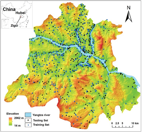
Figure 2. Landslide condition factor maps excluding elevation factor; the elevation factor map is shown in Figure 1. The legends of the lithology map: (1) water (2) loose soil (3) soft clay (4) soft and hard sandstone–claystone lithofacies (5) moderately hard to weakly soft conglomerate–sandstone lithofacies (6) hard thick-bedded sandstones (7) weakly karstified carbonates (8) moderately karstified carbonate (9) medium-strength karstified carbonate (10) strongly karstified carbonates (11) hard lava rocks (12) hard metamorphic rocks.

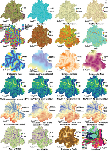
Table 1. The description and data source of landslide condition factors used in this study.

Factor (abbreviation)	Description and data source
(1) Elevation	Global SRTM DEM data with a spatial resolution of 1 arc-second (https://earthexplorer.usgs.gov).
(2) Slope	Using elevation data to generate different geomorphic components using Arcgis 10.6 software
(3) Terrain Ruggedness Index (TRI)
(4) Curvature
(5) Plan Curvature
(6) Profile Curvature
(7) Topographic Position Index (TPI)
(8) Topographic Wetness Index (TWI)
(9) Aspect
(10) Maximum 20-months Cumulative Rainfall (Rainfall_20), (11) Maximum 10-months Cumulative Rainfall (Rainfall_10), (12) Maximum one-month Cumulative Rainfall (Rainfall_1), (13) Average Annual Rainfall (Rainfall_Aver)	The data are calculated based on the 1-km monthly precipitation dataset for China (1901–2020). The dataset is provided by National Tibetan Plateau Data Center (https://data.tpdc.ac.cn/zh-hans/data/faae7605-a0f2-4d18-b28f-5cee413766a2/) (Peng et al. 2019)
(14) Multi-year Monthly Average NDVI (NDVI) (15) Neighborhood Statistics of Local Mean by 5 × 5 pixel window for (14) (NDVI_5), (16) Neighborhood Statistics of Local Mean by 9 × 9 pixel window for (14) (NDVI_9), (17) Neighborhood Statistics of Local Mean by 13 × 13 pixel window for (14) (NDVI_13)	The data was generated by GEE based on the period 1986–2020. Considering the growing season of plants in Zigui County and the contamination of images by clouds and snow, the mean-monthly NDVI values were first calculated by monthly averaging from May to October, and then by averaging the NDVI values for the six months obtained. In order to better suppress noise, the neighborhood Statistics of Local Mean were calculated based on multi-year monthly average NDVI using the focal statistics tool of Arcgis 10.6.
(18) Distance to Fault (Fault)	The data was from a 1:50,000 geological map (http://www.ngac.org.cn/, last accessed on 08/10/2022).
(19) Lithology	The data was from a 1:1000,000 Engineering Geological Map (https://geocloud.cgs.gov.cn, last accessed on 20/10/2022).
(20) Distance to River (River)	The data was generated by OpenStreetMap (OSM). (http://download.geofabrik.de/asia/, last accessed on 12/30/2022)
(21) Distance to River in the Reservoir Control Reach (Reservoir)
(22) Distance to Road (Road)
(23) Mean of NDBI (NDBI_Mean) (24) Max of NDBI (NDBI_Max)	The data was generated by GEE based on the period 1986–2020. Mean of NDBI refers to the multi-year mean of NDBI. Considering that anomalies exist in the maximum value of NDBI caused by the image stripes noise, Max of NDBI refers to the 95th percentiles of the statistical NDBI histogram
(25) Distance to Mine (Mine)	Mine data was provided by the National Mineralogical Database (http://data.ngac.org.cn/, last accessed on 12/30/2022) and by visual interpretation of Google history images.

Table 2. The causes of selecting the landslide condition factors used in this study.

Abbreviation of factor	Causes of selecting the factors
Elevation	It is anticipated that there will be a positive correlation between increasing elevation and a higher frequency of landslides. (Larsen and Torres-Sánchez 1998)
Slope	Studies have indicated that slope angle exerts a significant influence on landslides, with steeper slopes exhibiting a greater propensity for landsliding. (ROTH 1983; C.-T.; C.-T. Lee 2013)
TRI	That TRI had the highest positive correlation with landslide occurrence. (Jebur, Pradhan, and Shafapour Tehrany 2014; Xu et al. 2022)
Curvature	Hill slopes with a concave curvature have been found to possess a slightly higher susceptibility to landslides as compared to their counterparts with a convex curvature. (Ohlmacher 2007)
Plan Curvature	Plan curvature is governed by water flow divergence/convergence, influencing downslope water flow, erosion, deposition, and landslide. (Cheng et al. 2022)
Profile Curvature	Profile curvature controls water flow convergence/divergence, shaping the likelihood of landslide on the slope. (Cheng et al. 2022)
TPI	The topographic position index provides a stronger sense of where landslide material may end up. (Emberson et al. 2022)
TWI	TWI is crucial to evaluate rainfall-induced pore water pressure and its influence on landslides, reflecting a key factor. (Rahali and Houda 2022)
Aspect	Aspect’s influence on landslides is rooted in contrasting vegetation and root cohesion arising from varied solar insolation levels. (Abancó et al. 2021)
Rainfall_20, Rainfall_10, Rainfall_1, Rainfall_Aver	Landslide is strongly related to rainfall event parameters (duration, intensity, total rainfall). (Berti et al. 2012)
NDVI, NDVI_5, NDVI_9, NDVI_13	Vegetation cover has both positive and negative impacts on landslides. The roots can reinforce soil shear strength, mitigating creep and erosion. However, increased coverage may elevate runoff and gully erosion, and root splitting may trigger landsliding. (Y. Gao and Zhang 2022; Y. Liu et al. 2012)
Fault	Faults introduce slope material discontinuity, making distance to faults a critical factor in landslide susceptibility assessment. (Çevik and Topal 2003)
Lithology	Each lithology contributes differently to the development of landslides. (C. Caiyan and Qiao 2009)
River	Rivers impact terrain erosion and water seepage, thus are critical factors in landslide analysis due to their distance. (Çevik and Topal 2003)
Reservoir	Below the water level, the shear strength of the sliding zone is reduced by reservoir impoundment. (Du, Yin, and Lacasse 2013)
Road	Field observations indicate a robust spatial association between landslides and roads. (McAdoo et al. 2018)
NDBI_Mean, NDBI_Max	NDBI reflects impermeable features, such as settlements and roads, which impact water runoff and slope stability. Consequently, high NDBI areas are susceptible to landslides. (V. D. Pham et al. 2020)
Mine	The principal factor contributing to diverse geological hazards, including landslides, is surface deformation caused by mining activities. (Z. Liu, Mei, and Sun 2022)

3. Methods

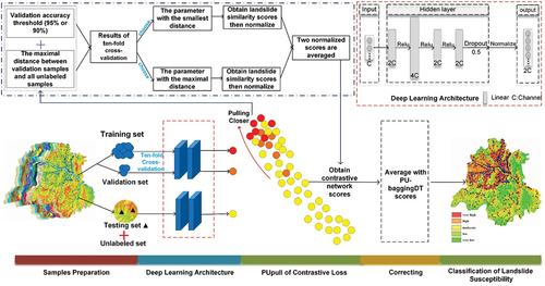
The approach in this paper focuses on calibrating the low accuracy results of PU-baggingDT with the scores learned from contrastive learning to obtain the classification probability of landslide susceptibility. The flow chart is shown in Figure 3. The model consists of a contrastive learning network and a PU-baggingDT model. Specifically, in step 1, all samples are divided into the training set, validation set, testing set and unlabeled set, where the training set, validation set and testing set are together composed of known landslide points, while the unlabeled set is composed of unknown landslide points. However, during training, the training and validation sets are known jointly as positive samples; the testing set is put into the unlabeled set and treated as an unlabeled dataset. In step 2, landslide susceptibility features are extracted by a contrastive learning network consisting of deep learning architecture and PUpull loss. Then, model parameters that represent the upper and lower bounds of the validation accuracy threshold are selected to generate two corresponding landslide similarity scores. Subsequently, each score is normalized, and the two resulting normalized scores are averaged to obtain a score of the contrastive learning network. In step 3, the average values of the contrastive learning network are averaged with the classification probability of PU-baggingDT to obtain the final values. In step 4, the results of the susceptibility score are categorized into five classes.

Figure 3. Detailed procedure of the PU-pullbaggingDT method.

3.1. The framework of the contrastive learning network

Our proposed contrastive network of landslides susceptibility only consists of an Encoder Network, which combines a deep learning architecture with the PUpull loss function. A tenfold cross-validation method and a set threshold of validation accuracy (95% or 90%) are applied to select the model parameters for the deep learning architecture. The deep learning architecture consists of four linear layers, with the first three linear layers activated by the ReLU function, a dropout layer, and a normalization layer, as shown in Figure 3. Among the four linear layers, the channel number of output features in each linear layer is twice, four times, twice, and twice the channel number of initial input features, respectively.

(1) $\mathit{Z}=\mathit{Normolize}\left(\mathrm{Dropout}\left(\mathrm{L}\left(\mathrm{Relu}\left(\mathrm{L}\left(\mathrm{Relu}\left(\mathrm{L}\left(\mathrm{Relu}\left(\mathrm{L}\left(\mathrm{x}\right)\right)\right)\right)\right)\right)\right)\right)\right)$(1)

Here, $\mathrm{Z}$ is the encoding of landslide susceptibility features and $\mathrm{L}$ is the linear layer for the linear transformation of the previous layer’s input. $\mathrm{Relu}$ represents the rectified linear unit. $\mathrm{Dropout}$ 0.5 is applied to prevent the architecture from overfitting and to improve its performance (Srivastava et al. 2014). $\mathrm{Normolize}$ is the normalization layer for mapping variables to between 0 and 1. It normalizes the features to be on the unit hypersphere (T. T. Wang and Isola 2020).

The PUpull loss of our proposed contrastive network is given as:

(2) $\mathcal{L}=\sum _{\mathit{i}\in \mathrm{P}}\mathit{\hspace{0.17em}}\left[-\log \frac{exp\left(\left({\sum }_{\mathit{p}\in \mathrm{P}\mathrm{\setminus }i}{\mathbf{z}}_i\cdot {\mathbf{z}}_p\right)/\left({\mathbf{N}}_p-1\right)\right)}{exp\left(\left({\sum }_{\mathit{p}\in \mathrm{P}\mathrm{\setminus }i}{\mathbf{z}}_i\cdot {\mathbf{z}}_p\right)/\left({\mathbf{N}}_p-1\right)\right)+{\sum }_{\mathit{u}\in \mathrm{U}}exp\left({\mathbf{z}}_i\cdot {\mathbf{z}}_u\right)}\right]$(2)

(3) $\mathcal{L}=\sum _{\mathit{i}\in \mathrm{P}}\mathit{\hspace{0.17em}}\left[-\log \frac{1}{1+\frac{{\sum }_{\mathit{u}\in \mathrm{U}}\mathit{exp}\left({\mathbf{z}}_i\cdot {\mathbf{z}}_u\right)}{\mathit{exp}\left({\mathbf{z}}_{\mathit{i}\cdot }\left({\sum }_{\mathit{p}\in \mathrm{P}\mathrm{\setminus }i}{\mathbf{z}}_p\right)/\left({\mathbf{N}}_p-1\right)\right)}}\right]$(3)

The training set and validation set consist of positive samples, along with the testing set, forming the entire collection of known landslide samples. $\mathrm{P}$ is referred to all training set. $\mathit{i}$ is one of $\mathrm{P}$. $\mathit{p}\in \mathrm{P}\mathrm{\setminus }\mathit{i}$ is one of training set but excluding $\mathit{i}$. ${\mathbf{N}}_p$ is the number of the training samples. $\mathrm{U}$ are all unlabeled samples (unknown landslide samples and testing set) for each batch. $\mathit{u}$ is one of $\mathrm{U}$. ${\mathbf{z}}_i$, ${\mathbf{z}}_p$, ${\mathbf{z}}_u$ are encoded by deep learning architecture for input samples $\mathit{i}$, $\mathit{p}$, $\mathit{u}$ respectively.

Based on equation 3(3) $\mathcal{L}=\sum _{\mathit{i}\in \mathrm{P}}\mathit{\hspace{0.17em}}\left[-\log \frac{1}{1+\frac{{\sum }_{\mathit{u}\in \mathrm{U}}\mathit{exp}\left({\mathbf{z}}_i\cdot {\mathbf{z}}_u\right)}{\mathit{exp}\left({\mathbf{z}}_{\mathit{i}\cdot }\left({\sum }_{\mathit{p}\in \mathrm{P}\mathrm{\setminus }i}{\mathbf{z}}_p\right)/\left({\mathbf{N}}_p-1\right)\right)}}\right]$(3) which is equivalent to equation 2(2) $\mathcal{L}=\sum _{\mathit{i}\in \mathrm{P}}\mathit{\hspace{0.17em}}\left[-\log \frac{exp\left(\left({\sum }_{\mathit{p}\in \mathrm{P}\mathrm{\setminus }i}{\mathbf{z}}_i\cdot {\mathbf{z}}_p\right)/\left({\mathbf{N}}_p-1\right)\right)}{exp\left(\left({\sum }_{\mathit{p}\in \mathrm{P}\mathrm{\setminus }i}{\mathbf{z}}_i\cdot {\mathbf{z}}_p\right)/\left({\mathbf{N}}_p-1\right)\right)+{\sum }_{\mathit{u}\in \mathrm{U}}exp\left({\mathbf{z}}_i\cdot {\mathbf{z}}_u\right)}\right]$(2) ,

$\mathit{exp}\left({\mathbf{z}}_{\mathit{i}\cdot }\left(\sum _{\mathit{p}\in \mathrm{P}\mathrm{\setminus }i}{\mathbf{z}}_p\right)/\left({\mathbf{N}}_p-1\right)\right)\mathit{\hspace{0.17em}}$is nearly equivalent to $\mathit{exp}\left({\mathbf{z}}_i\cdot {\mathbf{z}}_x\right)$, where ${\mathbf{z}}_x$ represents the mean of the sum of ${\mathrm{z}}_{\mathrm{p}}$. Specifically, this entails that sum of the similarities between positive sample ${\mathbf{z}}_i$ and each unlabeled sample should be less than similarity between the positive sample ${\mathbf{z}}_i$ and the mean of the overall training sample (analogous to the center of the positive sample projection). In contrast, the loss function does not impose this constraint on ${\mathbf{z}}_u$; thus, it has relaxed the tightness toward unlabeled samples. There are two reasons for this design: firstly, some unknown landslide samples are present in the unlabeled data, and secondly, the diverse features of non-landslide samples, which make their tight compression in the projection space unnecessary. The PUpull strategy only draws the training samples of positive samples closer, while forcing some of the unlabeled samples that are dissimilar to the training samples to move away from the positive ones. It differs from methods such as supervised contrastive (SupCon) (Khosla et al. 2020) and InfoNCE in that the penalty for positive and negative samples is strictly equal, while methods such as DCL use fixed class probability to impose different penalty strengths on positive and unlabeled samples.

However, as the PUpull loss continues to decrease, it may cause the training samples to become excessively compressed, resulting in a significant loss of landslide susceptibility information. Moreover, there is a risk of the algorithm overfitting the data, leading to potential issues of generalization. To address this issue, a tenfold cross-validation is employed to prevent overfitting of the network, and the degree of separation between positive samples and unlabeled samples is determined by the accuracy threshold of the validation set. It can be imagined that when the learning rate is set to a small value, the validation set in the first epoch of training is the most similar to the training set, and the validation accuracy is the highest, with the projection distance of the validation set being close to the unlabeled samples as well. The formula for the accuracy of the validation set is:

(4) $\begin{array}{c}\mathit{similarA}=\left(\sum _{\mathrm{i}=1}^{{\mathrm{N}}_P}\left(\mathrm{V}\cdot {\mathrm{P}}_{\mathrm{i}}\right)/\left(\left|\left|\mathrm{V}\right|\right|\cdot \left|\left|{\mathrm{P}}_{\mathrm{i}}\right|\right|\right)\right)/{\mathrm{N}}_P\end{array}$(4)

(5) $\begin{array}{c}\mathit{vali}{d}_{\mathit{ac}}=N_{\mathrm{similarA}>0}/N_{\mathit{valid}}\end{array}$(5)

where $\mathrm{V}$ is the encoding result of a single validation sample, ${\mathrm{P}}_{\mathrm{i}}$ is the encoding result of a single positive sample, and ${\mathrm{N}}_P$ is the number of positive samples. $N_{\mathrm{similarA}>0}$ is the number of samples in the validation set with similarity to the positive samples greater than zero. $N_{\mathit{valid}}$ represents the number of samples in the validation set.

As the network training progresses, the validation accuracy ($\mathit{vali}{d}_{\mathit{ac}}$) is expected to decrease gradually. When defining the validation accuracy threshold, it is important to consider the limitations of achieving a 100% validation accuracy, as it may lead to overfitting of the training samples and a lack of differentiation between positive and unlabeled samples. Additionally, the landslides in Zigui County have multiple causative factors, which means that not all positive samples can be accurately represented using a single network, this leads to some points being considered noise. To address this, we designated a subset of the validation set as noise points (5% or 10%). To ensure a high validation accuracy ($\mathrm{vali}{\mathrm{d}}_{\mathrm{ac}}$) while also staying away from the unlabeled data, during each cross-validation fold, an optimal model was selected based on the epoch that achieves the furthest distance from the unlabeled samples while maintaining a validation accuracy of 95% or 90%, respectively. The formula of distance from the unlabeled data is given as follows:

(6) $\begin{array}{c}\mathit{Distance}=\sum _{\mathit{a}=1}^{{\mathit{N}}_{\mathit{valid}}}\left[\left(\sum _{\mathrm{i}=1}^{{\mathrm{N}}_u}\left({\mathrm{V}}_{\mathrm{a}}\cdot {\mathrm{U}}_{\mathrm{i}}\right)/\left(\left|\left|{\mathrm{V}}_{\mathrm{a}}\right|\right|\cdot \left|\left|{\mathrm{U}}_{\mathrm{i}}\right|\right|\right)\right)/{\mathrm{N}}_u\right]\end{array}$(6)

where ${\mathrm{V}}_{\mathrm{a}}$ is the encoding result of a single validation sample, ${\mathrm{U}}_{\mathrm{i}}$is the encoding result of a single unlabeled sample, and ${\mathrm{N}}_u$is the number of unlabeled samples. $N_{\mathit{valid}}$represents the number of samples in the validation set.

Based on the tenfold cross-validation method, the number of model results obtained may be less than 10 at each fixed validation accuracy threshold. This is because the process of the loss reduction cannot guarantee achieving the specified validation accuracy in every cross-validation fold, potentially leading to direct transitions from high to low validation accuracies without achieving the intermediate fixed threshold. To ensure the reproducibility and stability of the stochastic model runs, for each specific validation accuracy threshold, the maximum and minimum values of the distance metric are selected among the model results. These two model results represent the upper and lower bounds of the possible distances between the positive and unlabeled samples that the given threshold can simulate.

For each of the two final model results, the similarity score for each sample is obtained by conducting a similarity comparison between the encoding result of each sample and that of the positive samples. Then, to ensure that the output result is close to the range [0,1] of PU-baggingDT, these scores are normalized using min-max scaling. The resulting normalized values from the two final model parameters are averaged to obtain the final score of the contrastive learning network. The formula is as follows:

(7) $\mathrm{scores}=\mathrm{Normolize}\left(\left({\sum }_{\mathrm{i}=1}^{{\mathrm{N}}_p}\left(\mathrm{A}\cdot {\mathrm{P}}_{\mathrm{i}}\right)/\left(\left|\left|\mathrm{A}\right|\right|\cdot \left|\left|{\mathrm{P}}_{\mathrm{i}}\right|\right|\right)\right)/{\mathrm{N}}_p\right)$(7)

(8) $\mathrm{score}{\mathrm{s}}_{\mathrm{contrastive}}=\left(\mathrm{score}{\mathrm{s}}_{\mathrm{Distanc}e-max}+\mathrm{score}{\mathrm{s}}_{\mathrm{Distance}-\min }\right)/2$(8)

where $\mathrm{A}$ is the encoding result of a single sample，and ${\mathrm{P}}_{\mathrm{i}}$ is the encoding result of a single positive sample. ${\mathrm{N}}_p$ is the number of positive samples, and $\mathrm{score}{\mathrm{s}}_{\mathrm{Distanc}e-max}$ refers to the normalized similarity scores, which are generated by the model that has maximum values of the Distance metric among the model results under a given threshold, while $\mathrm{score}{\mathrm{s}}_{\mathrm{Distance}-\min }$ is the opposite.

3.2. Calibration of probability scores for PU-baggingDT

Before correction, the results of the PU-baggingDT algorithm need to be acquired. PU-baggingDT was proposed by Bangyu et al. (2021). The number of iterations is set to 1000. In each iteration, a number of unlabeled samples equal to the number of positive samples are randomly selected as the negative samples and then input to the base classifier of the DecisionTree (DT) for training; the trained base classifier then gets the remaining classification scores that do not involve negative samples. In line with the concept of a bagging algorithm, the scores for each iteration are accumulated, after which, a reliable average is obtained.

After obtaining the values of PU-baggingDT, the scores of the contrastive learning network are then averaged with the output values of PU-baggingDT to generate the final output probability, which represents the likelihood of landslide occurrence for each cell.

(9) $\begin{array}{c}\mathit{Probability}=\left(\mathrm{score}{\mathrm{s}}_{\mathrm{contrastive}}+\mathrm{score}{\mathrm{s}}_{\mathrm{PU}-\mathrm{baggingDT}}\right)/2\end{array}$(9)

3.3. Classification of landslide susceptibility scores

Due to the various methods available for classifying landslide susceptibility scores in mapping, excluding subjective classification approaches, the prominent ones include quantile methods (Osaragi 2002), natural breaks (Jenks) (Jenks 1967), and equal interval (Osaragi 2002). The Quantile method allocates an equal number to each class, potentially leading to confusion as it combines low-probability susceptibility values with high-probability susceptibility values within the same class. Natural breaks (Jenks) aim to establish class boundaries that effectively group similar values while maximizing distinctions between classes. However, its breakpoint values may not accurately capture the true essence of landslide susceptibility scores within the range [0, 1]. The equal interval method is characterized by dividing the range of values into equal-sized subdivisions. Its breakpoints effectively emphasize one class of susceptibility relative to others within the fixed [0, 1] value range. Furthermore, compared to the other two methods, the equal interval method offers a more consistent standard for comparing different algorithms (Nandi and Shakoor 2010). Hence, based on the common practice of categorizing susceptibility scores into five levels by previous researchers (Fang et al. 2020; Guo et al. 2021), the equal interval method was ultimately utilized to classify the susceptibility scores into five levels, namely very high [0.80–1.00], high [0.60–0.80), moderate [0.40–0.60), low [0.20–0.40), and very low [0.00–0.20).

3.4. Precision evaluation

As negative samples are unknown, the accuracy measurement was performed solely on positive samples. The accuracy measurement focused on two primary aspects: (1) accuracy of classification for positive samples and (2) ranking performance for positive samples. This differs from previous works that usually considers only one of these evaluation metrics.

1. Producer accuracy (PA): PA measures the ratio of correctly classified landslide cells to the total number of reference landslide cells. The probability of correct classification is greater than or equal to 0.5. In this study, producer accuracy was evaluated separately for the testing dataset (Test_PA) and positive dataset (Train_PA).

2. Area under the curve (AUC) (Fang et al. 2021; S. Lee et al. 2003): AUC measures the relative ranking of landslide cells among all cells. First, the index values of all cells within the Zigui area were first sorted in descending order. Second, the sorted cells were divided into 100 intervals of equal numbers (I₁, I₂, I₃ … … .I₁₀₀). Third, the step involves tallying the number of landslide cells for the ith interval ($\sum _1^{\mathrm{i}}{\mathrm{N}}_{I_i}$), which is the sum of all landslide cell numbers that occurred between the first interval $({\mathrm{N}}_{I_1}$) and the current interval (${\mathrm{N}}_{I_i}$). Fourth, the AUC is computed by accumulating ratios, where each ratio represents the cumulative number of landslide cells in every interval divided by the total number of reference landslide cells ($N_{\mathit{total}}$), and then dividing the resulting sum by 100. The following formula is used:

   (10) $\begin{array}{c}\mathit{AUC}=(\sum _{\mathrm{i}=1}^{100}\left(\left(\sum _1^{\mathrm{i}}{\mathrm{N}}_{I_i}\right)/N_{\mathit{total}}\right))/100\end{array}$(10)

However, if there are many identical scores in the output scores of the landslide cells, even spanning many ranking intervals, simply accumulating and counting from the beginning of the ranking interval would result in a high AUC score, even though there may be a possibility of low overall landslide relative rankings. To more accurately reflect the relative ranking of landslide cell scores, we propose the “Left_AUC” and “Right_AUC” metrics. Left_AUC refers to the last ranking position of the same score when sorting landslide cell scores in descending order, and Right_AUC is the opposite, representing the first rank of the same score. For example, if the output score values of cells ranked from 100 to 300 are all 0.8, then the Left_AUC and Right_AUC ranks of the included landslides are 300th and 100th, respectively. In this study, “Left_AUC” and “Right_AUC” were evaluated separately for the testing dataset and positive dataset.

3.5. Experimental setup and environment

The data were divided into known landslide samples and unknown landslide samples, in which the known samples were 877 landslide points, 60% of which (526 raster cells, 474 for the training set and 52 for the validation set) were randomly selected as landslide-positive samples for training, while the remaining 2,758,117 raster cells were used as unlabeled samples, containing the remaining 40% (351 points) of the known landslide samples for testing. A tenfold cross-validation approach was employed. The StandardScaler was initially conducted by standardizing the factors, removing the mean and scaling to cell variance. The learning rate was 0.0001, and the epoch was set to 60. Owing to GPU memory limitations, the batch was set to 350,000 for unlabeled samples and all training set. Five average results with different random seeds were used for all experiments in this paper. All results were retained for up to four decimal places. The comparative analysis involved T-DNN, AdaPU-RF, and PU-baggingDT models, contrasting them with the PU-pullbaggingDT model based on three different validation accuracy thresholds. The code of AdaPU-RF was provided by the original author, and the parameter search and settings were based on the original publication. The codes for PU-baggingDT and T-DNN were reproduced independently, with parameters set of PU-baggingDT according to the same specifications as in the original work. Because the validation set had 52 samples, the proposed PU-pullbaggingDT employed three different validation set sizes, consisting of 52, 50, and 47 samples, to serve as threshold values for comparison, representing the validation accuracy of approximately 100%, 95%, and 90%, respectively. The following clarification needs to be made: setting the validation accuracy to 100% is solely for the purpose of facilitating a better understanding of the proposed model and does not imply that the model attains 100% validation accuracy. The PyTorch1.7 DL framework was used for the network. The experiments were implemented on Ubuntu 20.04.3 with GeForce RTX 3080.

4. Results

Table 3 shows that the results of PU-pullbaggingDT. When the threshold was 95% (valid50), Test_PA was 83.90%, with Right_AUC and Left_AUC at 78.51% and 78.50%, respectively. When the threshold was reduced to 90% (valid47), Test_PA fell by 3.97% to 79.93%, while both Right_AUC and Left_AUC increased by 0.02% to 78.75% and 78.74%, respectively. Figures 4 (a) and 4 (b) present the susceptibility distribution of PU-pullbaggingDT and the percentage of landslides, where landslides contain the training set, the validation set, and the test set. It was evident from the figures that more than 89% of landslides were located in very high and high susceptibility areas. In contrast, the very low susceptible and low susceptible areas contained less than 6% of all landslides in the region, with the percentages being 5.25% (valid47) and 3.87% (valid50), respectively. This indicates a high level of agreement between the distribution of landslides and the evaluation results of landslide susceptibility.

Figure 4. Landslide susceptibility map of the study area: (a) PU-pullbaggingDT_valid47 (b) PU-pullbaggingDT_valid50 (c) PU-pullbaggingDT_valid52 (d) PU-baggingDT (e) AdaPU-RF.

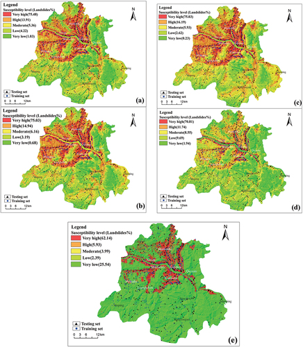
Table 3. Accuracy results of different models for the PU dataset in Zigui county. The range [×-×] refers to cells whose output scores fall within this range. “PCT” is an abbreviation for percentage, and “PCT of cells” refers to the cells within the score range [×-×] that occupy a percentage of all cells within Zigui county. Test_R_PA refers to the percentage of correct predictions in the testing set within the score range [×-×]. valid47, valid50, and valid52 refer to the selected validation accuracy threshold of 47/52, 50/52, and 52/52, respectively.

Model		AdaPU-RF(%)	PU-baggingDT(%)	（ours）PU-pullbaggingDT(%)
				valid47	valid50	Valid52
Testing set (351 raster cells)	Test_PA	51.79 ± 2.80	67.98 ± 0.61	79.93 ± 1.79	83.90 ± 1.45	87.37 ± 0.75
	Right_AUC	89.21 ± 0.44	78.66 ± 0.04	78.75 ± 0.13	78.51 ± 0.15	78.32 ± 0.04
	Left_AUC	52.79 ± 2.05	78.60 ± 0.04	78.74 ± 0.13	78.50 ± 0.15	78.31 ± 0.04
Training set and validation set (526 raster cells)	Train_PA	84.87 ± 0.76	100.00 ± 0.00	100.00 ± 0.00	100.00 ± 0.00	100.00 ± 0.00
	Right_AUC	93.54 ± 0.40	100.00 ± 0.00	97.59 ± 0.13	97.29 ± 0.23	97.70 ± 0.11
	Left_AUC	77.53 ± 0.61	100.00 ± 0.00	97.59 ± 0.13	97.29 ± 0.23	97.7 ± 0.11
[0.80–1.00]	PCT of cells	14.49 ± 0.58	4.05 ± 0.01	12.95 ± 0.15	13.30 ± 0.14	13.31 ± 0.05
	Test_R_PA	50.03 ± 1.72	26.84 ± 0.42	48.66 ± 0.64	49.85 ± 0.49	49.64 ± 0.44
[0.60–0.80)	PCT of cells	0.57 ± 0.14	12.91 ± 0.02	17.98 ± 1.11	22.16 ± 1.46	25.20 ± 0.52
	Test_R_PA	0.97 ± 0.86	29.86 ± 0.33	24.91 ± 0.72	27.08 ± 1.07	29.19 ± 0.55
[0.40–0.60)	PCT of cells	0.92 ± 0.20	21.83 ± 0.06	17.70 ± 1.04	22.75 ± 1.71	28.71 ± 1.18
	Test_R_PA	1.37 ± 0.58	21.42 ± 0.38	12.71 ± 1.06	13.45 ± 0.51	14.19 ± 0.39
[0.20–0.40)	PCT of cells	2.46 ± 0.43	30.27 ± 0.11	28.70 ± 0.26	26.83 ± 1.53	26.03 ± 0.47
	Test_R_PA	2.96 ± 0.53	16.87 ± 0.33	10.29 ± 0.83	7.76 ± 0.99	6.29 ± 0.20
[0.00–0.20)	PCT of cells	81.57 ± 1.26	30.93 ± 0.12	22.67 ± 2.28	14.96 ± 2.06	6.76 ± 1.20
	Test_R_PA	44.67 ± 3.07	5.01 ± 0.29	3.43 ± 0.68	1.87 ± 0.14	0.7 ± 0.29

5. Discussion

5.1. Different model accuracy analysis

A comparison of performance is presented in Table 3 for AdaPU-RF, PU-baggingDT, and PU-pullbaggingDT. Regarding the testing set, AdaPU-RF achieved the highest Right_AUC score of 89.21%, which exceeded the second highest score of 10.55% obtained by PU-baggingDT. However, its Left_AUC and Test_PA were the lowest among all models, reaching only 52.79% and 51.79%, respectively. Additionally, it was observed that 44.67% of testing samples fell within the score range of [0.00–0.20). These results suggest that the ranking performance of AdaPU-RF on the testing set is not very high. It can also be observed from Figure 4(e) that the results predicted by AdaPU-RF are mainly distributed around the Yangtze River and its tributaries, which is the area with the highest density of known landslide samples. This may be due to the fact that AdaPU-RF is able to select the least likely 10% of unlabeled samples as negative samples, and although it greatly improves the accuracy and ranking of the primary causes of Zigui landslide identification, there are no suitable negative samples selected for secondary causes of multi-causal Zigui landslide. Compared with PU-baggingDT, Right_AUC and Left_AUC of PU-baggingDT were closer, and the mean value of both is greater than that of AdaPU-RF 7.63%, indicating a higher ranking in its testing set. It may be because PU-baggingDT selects different batches of negative samples to learn different landslide susceptibility features, which is beneficial to the identification of landslides with multiple geneses in Zigui. However, the proportion of actual positive instances in the unlabeled dataset may be higher, leading to the misclassification of negative samples by PU-baggingDT and resulting in a lower Test_PA accuracy. In response, the contrastive network of proposed PU-pullbaggingDT was introduced to correct the Test_PA accuracy of PU-baggingDT. Using this approach, the highest Test_PA accuracy of valid52 is 87.37%, which is higher than PU-baggingDT by 19.39%, but the Right_AUC and Left_AUC of valid52 were lower, though only 0.34% and 0.29% lower than those of PU-baggingDT, respectively. Furthermore, from the perspective of various predicted score ranges, the improved Test_ PA of PU-pullbaggingDT led to an increase in high susceptibility areas. The very high and high susceptibility landslide area [0.40–0.60) for valid52 accounts for 38.51% of the total, showing an increase of 21.55% compared to PU-baggingDT. Notably, an improvement of valid52 in the Test_R_PA accuracy of 22.13% was also observed in these two regions. As the chosen validation accuracy threshold decreased, Test_PA also decreased, but the Test_PA of valid47 remained higher than that of PU-baggingDT 11.95%, while Right_AUC and Left_AUC of valid47 increased, being higher than those of PU-baggingDT by 0.09% and 0.14%, respectively. The very high and high susceptibility areas of valid47 also decreased compared to those of valid52, but still increased by 13.97% compared to those of PU-baggingDT. Moreover, the Test_R_PA accuracy of valid47 in these two regions also increased by 16.87% compared to that of PU-baggingDT. Although the PU-pullbaggingDT method makes the very high and high susceptibility landslide area increase, the prediction accuracy of the testing set is also greatly improved with almost no reduction in the prediction sample ranking. The theory of correction will be discussed in Section 5.4.

Because default parameters may not fully capture the model’s advantages when transferred to a new region, this section explores the results of all comparative models under different parameters. The original work of AdaPU-RF provided an extensive range of search parameters, and the results presented in this study are based on the outcomes of parameter searches, with further discussion on this matter omitted. For PU-baggingDT, the sole variable is the number of base learners, set to quantities of 500, 800, 1300, and 1500. When compared to the original default parameter of 1000 for base learners, results in Table 4 indicate minimal differences in accuracy, with the maximum observed differences being approximately 0.1% for Test_Right_AUC and Test_Left_AUC, and a maximum difference of 0.86% for Test_PA. Therefore, the final parameter setting aligns with the original default parameter of 1000 as specified in the original study. For T-DNN, it consists of two deep learning training stages, referred to in this study as stage 1 and stage 2. Stage 1 is dedicated to identifying the threshold for spy selection. Stage 2 involves training using chosen negative samples and the positive samples (526 raster cells). All parameters aligned with the original study, with variations only in the number of experimental epochs. As depicted in Figure 5(a), with these parameters, the loss remained stable at approximately 230 epochs during stage 1, and in stage 2, the performance of the change in loss at different results of stage 1 is nearly identical, it reached stability around 60 epochs. Additionally, the loss in both stages was able to reach zero. This suggests that the parameters were suitable for Zigui region. Moreover, the quantity of randomly selected negative samples in both stage 1 and stage 2 equals the number of positive training samples used. Based on the performance of epochs with stable loss and loss approaching 0, accuracy was computed for Stage 1 within the range of epochs 1 to 250 at intervals of 5 epochs. Similarly, for stage 2, 50th and 70th epochs to represent the stable epoch of loss, while also including the 30th epoch for comparison. Observing Figure 5, it can be noted that the Test_PA of T-DNN at epochs 50th and 70th in stage 2 is consistently above 95%, surpassing the valid_47 by approximately 16%-20%. Although the Left_AUC of T-DNN was slightly lower than valid_47 by around 5–12%, and the Right_AUC was lower by about 2–6%. From these results, T-DNN appeared to perform well. However, observations from Figures 6(b,c) reveal that at the 50th and 70th epochs, the probability scores across Zigui County exhibit a pattern where nearly 90% of the raster cells fall within the range of [0.6–1]. This implies that 90% of the area is deemed at high risk of landslides, which contradicts the actual scenario and may be indicative of overfitting in the network. Additionally, from Figure 6(a), it can be observed that, at the 30th epoch of Stage 2, the majority of results are distributed in the range of [0.2–0.8], indicating less conspicuous signs of overfitting. However, the loss at the 30th epoch of Stage 2 is not in a stable phase, contradicting the approach proposed in the original text, which advocated selecting epochs based on stable loss. Therefore, the proposed model was not compared in detail with T-DNN. This also indirectly suggests that the negative samples chosen through the spy method in this area fail to sufficiently separate positive and negative instances, resulting in overall probability scores that are relatively close. Of course, it should be noted that this code of experiment, being a reproduction, may not entirely represent the original approach.

Figure 5. (a) The loss of D-TNN in different stage. (b) The Test_PA of D-TNN at the 30th/50th/70th epoch of stage 2. (c) The Test_Left_AUC of D-TNN at the 30th/50th/70th epoch of stage 2. (d) The Test_Right_AUC of D-TNN at the 30th/50th/70th epoch of stage 2.

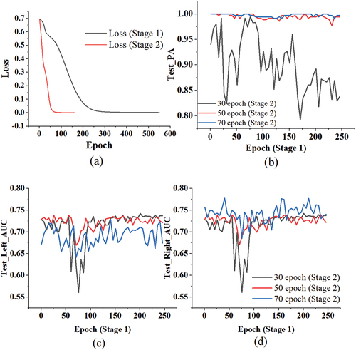
Figure 6. The probabilistic classification results of all cells within Zigui county at the 30th/50th/70th epoch of stage 2 for D-TNN.

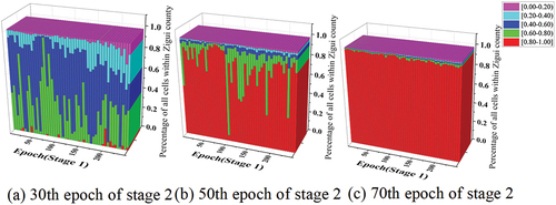
Table 4. Accuracy results of different models for the PU dataset in Zigui county. Test_Right_AUC and Test_left_AUC refer to the AUC results based on the testing set.

Epochs of iterations	Test_Right_AUC	Test_Left_AUC	Test_PA
500	78.68 ± 0.15	78.54 ± 0.14	67.12 ± 0.76
800	78.61 ± 0.05	78.55 ± 0.04	67.29 ± 0.75
1300	78.75 ± 0.05	78.71 ± 0.06	67.86 ± 0.49
1500	78.72 ± 0.08	78.69 ± 0.08	67.52 ± 0.36
1000(original parameter)	78.66 ± 0.04	78.60 ± 0.04	67.98 ± 0.61

5.2. Comparison of landslide susceptibility mapping results from different models

Figure 4 shows susceptibility distribution and the percentage of landslides, where landslides contain the training set, the validation set, and the test set. The results used the median PA accuracy from five experiments. It was obvious that after correction, the percentages of landslides in very high and high susceptibility areas of PU-pullbaggingDT from (a) to (c) were 89.39%, 89.97%, and 91.22%, respectively, which was 6.84%, 7.42%, and 8.67% higher than that of PU-baggingDT. It reflected the higher percentage of landslides in very high and high susceptible areas after correction, but their corresponding areas of 31.3%,35.24%, and 38.32% were 14.35%,18.29%, and 21.37% higher, respectively, than that of PU-baggingDT (16.95%). The reason for this was that the PU-baggingDT algorithm has a 100% AUC for the training and validation set, meaning that the scores of positive samples are located at the forefront of all samples. Additionally, the positive samples accounted for 60% of the total percentage of landslide samples. This allowed the result of PU-baggingDT to cover a relatively large proportion of landslides within a small area, even when the Test_PA accuracy was not high. In addition, Xudong et al. (2021) (Xudong et al. 2021) proposed a supervised ensemble algorithm (BRSNBtree) in Zigui County, which used 70% of the known landslide samples for training. The predicted landslide proportions and corresponding areas of very high and high susceptible areas were 76.46% and 39.99%, respectively. The proportions of landslides were lower than those predicted by the PU-pullbaggingDT algorithm (using 60% of the known landslide samples) by 12.93%, 13.51%, and 14.76%, whereas the corresponding area proportions were higher by 8.69%, 4.57%, and 1.67%, respectively. The results demonstrated that the dataset and algorithm designed in this study can better fit the landslide susceptibility features and achieve higher landslide prediction proportions with less predicted area.

5.3. Reason for integration algorithm

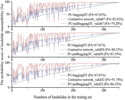
Explanation of the integration methodology is essential following the algorithm results. There are a number of diverse features involved in determining the susceptibility to landslides in Zigui County, such as the fact that landslides near the Yangtze River are affected by reservoir fluctuations, while those far from it are less affected. It can also be said that the category of landslide susceptibility features contains multiple distinct subcategories. The PU-baggingDT algorithm employs a bagging strategy to randomly select different negative samples and create multiple predictors that learn different landslide susceptibility subcategory features, thus providing noise robustness and achieving optimal ranking performance against existing PU learning outcomes for landslide susceptibility prediction. However, the presence of label bias in PU data can lead to the inclusion of positive samples in the negative samples randomly selected from the unlabeled data, resulting in decreased prediction accuracy and high bias. Specifically, in this study, only the center points of landslide mass were selected as samples, and there were many large landslides in Zigui County, indicating the existence of many positive landslide samples in the unlabeled data, which increases the risk of sample misselection. To improve the prediction accuracy of PU-baggingDT, we designed a contrastive network to correct its predictions. The purpose of the contrastive network is to reduce the projection distance of limited positive landslide samples to improve the prediction accuracy. However, setting a high validation accuracy may result in a close similarity between positive and negative samples, which may introduce more noise in the predicted landslide features and lead to a low ranking in the prediction results, which is in contrast to the PU-baggingDT feature. To obtain a result with low bias and high ranking performance, the two methods were integrated to improve the robustness of the prediction. The result of a random run, as shown in Figure 7, indicates that the PU-pullbaggingDT outcome is calibrated in terms of Right_AUC performance on the testing set. PU-baggingDT exhibits superior Right_AUC performance compared to the contrastive network, particularly on the highest-ranked samples (representing the main causal factors of landslides). This indicates that PU-baggingDT exhibits lower noise in identifying the primary causal factors of landslides compared to the contrastive network. Moreover, as the threshold of validation accuracy increases, the contrastive network shows poorer ranking performance for the primary causal landslide samples, whereas PU-baggingDT exhibits better calibration of Right_AUC performance. The calibration scores for Right_AUC for valid52, as shown in Figure 7, reached 4.80%, which is 1.53% and 2.42% higher than those for valid50 and valid47, respectively. The effect of the corrected Test_PA accuracy is shown in Figure 8. As the validation accuracy threshold increases, Test_PA of PU-baggingDT is corrected by the contrastive network with scores of 11.39%, 15.38%, and 18.51%.

Figure 7. The Right_AUC results of contrastive network for testing set were calibrated by PU-baggingDT.

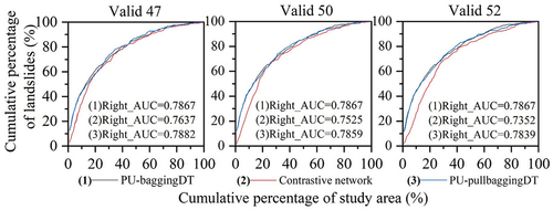
Figure 8. The low accuracy results of PU-baggingDT for the testing set were calibrated using the contrastive network.

5.4. Impact of different validation accuracies on the accuracies of the contrastive network

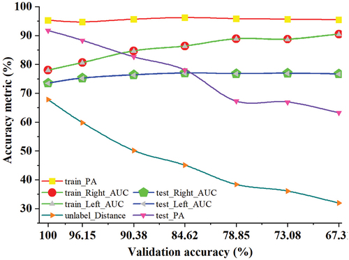
To further illustrate the performance of the contrastive network, one randomly selected run produced the results shown in Figure 9. This figure depicts the performance of the contrastive network across various validation accuracy thresholds, spanning from 67.31% (35 samples) to 100% (52 samples). As the validation accuracy threshold decreases, the Left_AUC and Right_AUC accuracies of the positive samples gradually increase, whereas Train_PA remains stable with small fluctuations. This indicates that the positive samples are gradually ranked higher in the overall sample set. In contrast, the distance between the unlabeled samples and positive samples increases, and the Test_PA decreases as well. This suggests that as the unlabeled data moves further away from the positive samples, there is a gradual loss of landslide susceptibility information, which leads to a decrease in the PA of the testing set. However, the Left_AUC and Right_AUC performance on the testing set does not decrease simultaneously with the decrease in Test_PA, but rather gradually improves and then slightly decreases. This may be due to the fact that as the positive samples are pulled in by the positive samples center, the primary features related to landslide susceptibility are increasingly uncovered.

Figure 9. Impact of different validation accuracies on the accuracies of the contrastive network for the testing set.

5.5. Impact of removing highly correlated factors on accuracies

Previous studies have suggested that strong linear correlations between factors can introduce noise and negatively impact the accuracy of machine learning models. In order to further investigate the impact of highly correlated factors on PU learning model accuracy, the conditioning factors with high-correlation and low importance were removed from the dataset by using the Spearman Correlation Index and Gini coefficient of RF. The Spearman Correlation Index is commonly used to measure multicollinearity between two variables, with an absolute coefficient greater than 0.7 indicating a strong linear correlation between two factors (Passman et al. 2011). The importance ranking of factors was measured by calculating the Gini coefficient in RF (Boulesteix et al. 2012). Since no predefined negative samples were available, 1000 sets of negative samples were randomly selected. Each set of negative samples was used to calculate the importance ranking score, and the final score was determined by averaging the scores from all iterations.

Figure 10 displays the results of feature importance ranking, and it was evident from the graph that the top two contributing factors were NDVI_9 and Profile Curvature. Based on the results of the Spearman correlation coefficient (<0.7) (Figure 11) and the ranking of factor importance, 12 factors were retained, including NDVI_9, Profile Curvature, Rainfall_10, Aspect, Fault, Mine, Slope, River, TWI, Lithology, NDBI_Max, and Road. Table 5 shows the results of the models after retraining using these factors. Compared with Table 3, concerning the AUC metric on the test set, all models exhibit a decline in AUC accuracy. AdaPU-RF showed the largest decrease in Left_AUC (4.28%), followed by PU-pullbaggingDT_valid47 (1.89%), PU-pullbaggingDT_valid52 (1.67%), PU-pullbaggingDT_valid50 (1.41%), and PU-baggingDT (1.07%). It may be because the removed factors still contain information beneficial to the relative ranking. In terms of the test_PA metric, only PU-pullbaggingDT_valid47, PU-pullbaggingDT_valid52, and PU-pullbaggingDT_valid50 exhibit improvements, with increases of 2.88%, 1.22%, and 0.83%, respectively. The remaining models experienced a decline, with AdaPU-RF showing the most significant decrease at 2.1%. These results indicated that removing highly correlated factors tends to have an overall detrimental impact on the ranking performance of PU algorithms. However, it was worth noting that the proposed PU-pullbaggingDT algorithm achieved higher accuracy in predicting landslide probability scores.

Figure 10. Feature importance ranking of 25 conditioning factors, the abbreviations for the names are listed in Table 2.

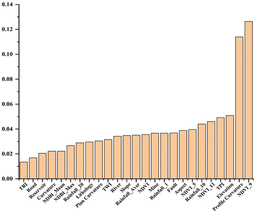
Figure 11. Spearman correlation coefficient of 25 conditioning factors, the abbreviations for the names are listed in Table 2.

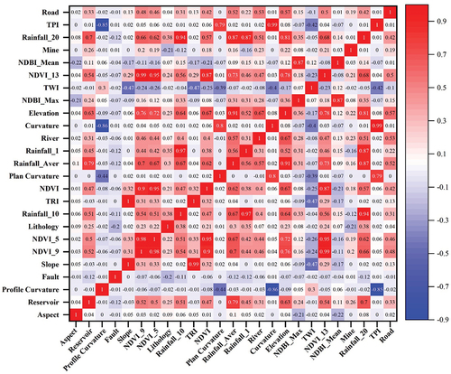
Table 5. Accuracy results of different models for the remaining 12 factors.

		AdaPU-RF	PU-baggingDT	（ours）PU-pullbaggingDT
				valid47	valid50	valid52
Testing set	Test_PA	49.69 ± 1.15	66.67 ± 0.40	82.81 ± 0.09	84.73 ± 0.12	88.59 ± 0.1
	Right_AUC	89.13 ± 0.33	77.59 ± 0.10	76.86 ± 0.06	76.84 ± 0.06	76.91 ± 0.07
	Left_AUC	48.51 ± 0.71	77.53 ± 0.11	76.85 ± 0.06	76.83 ± 0.06	76.90 ± 0.07
Training set and validation set	Train_PA	84.26 ± 0.25	100.00 ± 0.00	100.00 ± 0.00	100.00 ± 0.00	100.00 ± 0.00
	Right_AUC	93.76 ± 0.24	100.00 ± 0.00	97.35 ± 0.01	97.61 ± 0.01	98.25 ± 0.01
	Left_AUC	76.75 ± 0.92	100.00 ± 0.00	97.35 ± 0.00	97.61 ± 0.01	98.25 ± 0.01

5.6. Impact of random selection of negative samples on accuracy

To further illustrate the proposed method that does not involve selecting negative samples for the study of the Zigui area, compare the results of supervised algorithms, which necessitates the selection of negative samples. The supervised algorithm was based on the most widely used method of randomly selecting landslide-negative samples (Dou et al. 2020; Tsangaratos et al. 2017), five sets of negative samples with the same number of positive samples were randomly chosen as shown in Figure 12. SVM, RF, LR, AdaBoost, and XGBoost are commonly used supervised algorithms that require negative samples. These algorithms were utilized for the analysis, and the optimal validation accuracy was determined through parameter search and ten-fold cross-validation. The search parameters and test results of the five runs are presented in Table 6. The accuracy metrics showed some variations, with the Test_PA of the SVM having the largest variation, up to 10.26%. From Table 6, it can be observed that the proposed method outperforms various machine learning models based on randomly selected negative samples in terms of Test_PA and Left_AUC. Specifically, the Test_PA for valid47 and valid50 was higher by 8.7% and 12.67%, respectively, compared to the highest Test_PA in Table 6. Additionally, the Left_AUC was higher by 0.29% and 0.05%, respectively, compared to the highest Test_PA in Table 6. However, in terms of Right_AUC, the proposed method is lower by 0.69% and 0.93% compared to the highest Right_AUC in Table 6. Nevertheless, in terms of overall accuracy, landslide susceptibility mapping results, and stability in identifying multi-factor landslide susceptibility in Zigui County, the proposed method exhibits superior performance over various machine learning models based on randomly selected negative samples.

Figure 12. Sampling positions of five randomly selected negative samples.

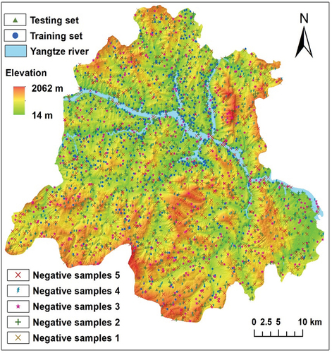
Table 6. Accuracy results of various machine learning models on five randomly selected negative samples.

		1	2	3	4	5
Test_PA (%)	SVM	70.09	59.83	66.38	62.68	70.09
	LR	69.8	64.1	66.67	64.96	68.09
	RF	68.66	66.38	63.25	62.96	67.24
	AdaBoost	66.67	66.67	71.23	68.09	67.24
	XGBoost	70.09	66.67	60.4	65.81	68.66
Left_AUC (%)	SVM	73.35	75.19	75.07	74.63	75.26
	LR	74.86	75.42	74.6	74.32	74.58
	RF	77.91	78.19	75.99	78.45	78.27
	AdaBoost	74.58	74.55	72.92	75.9	75.04
	XGBoost	76.07	77.76	74.5	78.35	77.82
Right_AUC(%)	SVM	73.38	75.21	75.08	74.66	75.3
	LR	74.88	75.42	74.6	74.33	74.59
	RF	78.17	79.44	77.79	78.62	78.63
	AdaBoost	75.05	74.86	78.39	78.07	75.35
	XGBoost	76.09	77.77	74.52	78.36	77.83
Train_PA (%)	SVM	75.86	70.91	78.14	77.76	82.32
	LR	78.33	72.05	73.95	72.62	78.14
	RF	98.1	98.1	98.67	98.48	98.29
	AdaBoost	89.54	81.75	80.42	78.71	81.56
	XGBoost	99.05	98.48	99.24	83.08	95.06
Search space	SVM	C: [0.1, 1, 10, 100, 1000]; gamma [10, 1, 0.1, 0.001, 0.0001]
	LR	Penalty: [L1, L2]; C [0.001.0.01.0.1.1.10, 100]
	RF	Number of trees: [10, 20, 30, …, 100] and [100, 150, 200, …, 500]
	AdaBoost	n_estimators: [10, 20, 30, …, 100] and [100, 150, 200, …, 500]; learning_rate :[0.125, 0.25, 0.5, 1, 2]
	XGBoost	n_estimators: [50, 100, 150, 200, 300]; max_depth: [3, 4, 5, 6, 7]; colsample_bytree: [0.4, 0.6, 0.8, 1]; min_child_weight: [1, 2, 3, 4]; learning_rate :[0.05, 0.1, 0,2, 0.3]

5.7. Analysis of precision results in comparison to other regions

Compared with research results in certain regions, the PA values in this area are relatively lower. This could be attributed to one potential reason: Many studies artificially categorize the factors of continuous data during input data preprocessing, whereas all continuous data in this paper undergo no artificial categorization. For instance, in the Changbai Mountain Area using the T-DNN algorithm, all continuous factors are divided into five or seven classes before network training. Similarly, in the study area based on the PU-baggingDT algorithm, all continuous samples are divided into five classes. To some extent, this method can mitigate the complexity of the network in learning the landslide susceptibility factors. This is because, during the factor division, some landslide samples are already classified into some specific categories, eliminating the need for the network to explore the numerical ranges representing landslide susceptibility levels from various values. Similarly, the categorization has also assisted in classifying landslide-negative samples into some specific categories, indirectly aiding in the selection of negative samples. However, adopting such a method can lead to results with a certain degree of subjective bias. This is because the results would categorize areas prone to landslides based on the artificially defined range of factors, potentially causing some areas with lower landslide probability to be erroneously classified as susceptible. In response to this issue, all continuous data in this paper is directly inputted, avoiding artificial categorization.

5.8. Limitations and future scope of the research

It is important to acknowledge this study has certain limitations. The spatial resolution of the factors may not be fine enough, and some crucial factors might not have been collected, which could result in less precise and less accurate prediction outcomes. Additionally, when utilizing long-term data, the proposed approach faces limitations. The occurrence probability of some landslides may decrease post-event, but the long-term data considers circumstances afterward, potentially causing data anomalies. Furthermore, there is a lack of interpretability analysis regarding the network’s performance in landslide susceptibility prediction, posing a challenge in understanding to comprehend how the network arrives at its predictions.

In the future, efforts will be directed toward enhancing the interpretability of the network and applying the algorithm to different geographical areas to assess its generalization and spatial transferability. Additionally, in the direction of PU learning, if it is possible to utilize knowledge graphs or relationships between factors to augment landslide factor data and maintain the semantic invariance of landslide susceptibility, it can further promote the learning of key features for landslide susceptibility through PU learning.

6. Conclusions

This study proposes a new algorithm, called PU-pullbaggingDT, specifically designed for the multi-causal landslides in Zigui. The algorithm is an integration of the high ranking PU-baggingDT algorithm with and low bias contrastive learning. In comparison to PU-baggingDT, this integration significantly increases the prediction accuracy by 11.95%-19.39% without decreasing the PU-baggingDT AUC too much (+0.14 to −0.43). Within the proposed algorithm, a new contrastive loss, called “PUpull,” is introduced for PU learning. This loss function, implemented without the need for data augmentation and class probability, helps to pull the spatial projection distance between landslide samples closer while being less affected by incorrectly defined negative samples, resulting in a low bias outcome. The proposed algorithm outperforms current landslide-based PU-learning algorithms and machine learning algorithms that rely on randomly selected negative samples.

Acknowledgments

This work was jointly supported by the Key R & D plan of Hubei Province (NO.2021BID009), the Fundamental Research Funds for the Natural Science Foundation of China (No. U21A2013), the Opening Fund of Key Laboratory of Geological Survey and Evaluation of Ministry of Education (Grant No. GLAB2022ZR02) and the Fundamental Research Funds for the Central Universities.

This work was also supported by the High-performance GPU Server (TX321203) Computing Center of the National Education Field Equipment Renewal and Renovation Loan Financial Subsidy Project of China University of Geosciences, Wuhan.

Disclosure statement

The authors declare that they have no known competing financial interests or personal relationships that could have appeared to influence the work reported in this paper.

Data availability statement

We present the codes openly available at https://github.com/ShubingOuyangcug/PU-pullbaggingDT to encourage reproducibility of the study.

Additional information

Funding

This work was supported by the the Key R & D plan of Hubei Province [NO.2021BID009]; the Fundamental Research Funds for the Natural Science Foundation of China [No.U21A2013]; the Opening Fund of Key Laboratory of Geological Survey and Evaluation of Ministry of Education [Grant No.GLAB2022ZR02].

References

- Abancó, C., G. L. Bennett, A. J. Matthews, M. A. M. Matera, and F. J. Tan. 2021. “The Role of Geomorphology, Rainfall and Soil Moisture in the Occurrence of Landslides Triggered by 2018 Typhoon Mangkhut in the Philippines.” Natural Hazards and Earth System Sciences 21 (5): 1531–24. Copernicus GmbH. https://doi.org/10.5194/nhess-21-1531-2021.
- Acharya, A., S. Sanghavi, L. Jing, B. Bhushanam, D. Choudhary, M. Rabbat, and I. Dhillon. 2022. “Positive Unlabeled Contrastive Learning.” arXiv preprint arXiv:2206.01206.
- Aleotti, P., and R. Chowdhury. 1999. “Landslide Hazard Assessment: Summary Review and New Perspectives.” Bulletin of Engineering Geology and the Environment 58 (1): 21–44. https://doi.org/10.1007/s100640050066.
- Al-Najjar Husam, A. H., B. Pradhan, B. Kalantar, M. I. Sameen, M. Santosh, and A. Alamri. 2021. “Landslide Susceptibility Modeling: An Integrated Novel Method Based on Machine Learning Feature Transformation.” Remote Sensing 13 (16): 3281. Multidisciplinary Digital Publishing Institute. https://doi.org/10.3390/rs13163281.
- Bangyu, W., W. Qiu, J. Jia, and N. Liu. 2021. “Landslide Susceptibility Modeling Using Bagging-Based Positive-Unlabeled Learning.” IEEE Geoscience and Remote Sensing Letters 18 (5): 766–770. https://doi.org/10.1109/LGRS.2020.2989497.
- Berti, M., M. L. V. Martina, S. Franceschini, S. Pignone, A. Simoni, and M. Pizziolo. 2012. “Probabilistic Rainfall Thresholds for Landslide Occurrence Using a Bayesian Approach.” Journal of Geophysical Research: Earth Surface 117 (F4). https://doi.org/10.1029/2012JF002367.
- Boulesteix, A.-L., A. Bender, J. Lorenzo Bermejo, and C. Strobl. 2012. “Random Forest Gini Importance Favours SNPs with Large Minor Allele Frequency: Impact, Sources and Recommendations.” Briefings in Bioinformatics 13 (3): 292–304. https://doi.org/10.1093/bib/bbr053.
- Budimir, M. E. A., P. M. Atkinson, and H. G. Lewis. 2015. “A Systematic Review of Landslide Probability Mapping Using Logistic Regression.” Landslides 12 (3): 419–436. https://doi.org/10.1007/s10346-014-0550-5.
- Caiyan, W., and J. Qiao. 2009. “Relationship Between Landslides and Lithology in the Three Gorges Reservoir Area Based on GIS and Information Value Model.” Frontiers of Forestry in China 4 (2): 165–170. https://doi.org/10.1007/s11461-009-0030-6.
- Çevik, E., and T. Topal. 2003. “GIS-Based Landslide Susceptibility Mapping for a Problematic Segment of the Natural Gas Pipeline, Hendek (Turkey).” Environmental Geology 44 (8): 949–962. https://doi.org/10.1007/s00254-003-0838-6.
- Cheng, J., X. Dai, Z. Wang, L. Jingzhong, G. Qu, L. Weile, J. She, and Y. Wang. 2022. “Landslide Susceptibility Assessment Model Construction Using Typical Machine Learning for the Three Gorges Reservoir Area in China.” Remote Sensing 14 (9): 2257. Multidisciplinary Digital Publishing Institute. https://doi.org/10.3390/rs14092257.
- Chen, W., L. Xianju, Y. Wang, G. Chen, and S. Liu. 2014. “Forested Landslide Detection Using LiDAR Data and the Random Forest Algorithm: A Case Study of the Three Gorges, China.” Remote Sensing of Environment 152 (September): 291–301. https://doi.org/10.1016/j.rse.2014.07.004.
- de Campos, M. Luis, M. F.-L. Juan, F. H. Juan, and L. Redondo-Expósito. 2018. “Positive Unlabeled Learning for Building Recommender Systems in a Parliamentary Setting.” Information Sciences 433–434 (April): 221–232. https://doi.org/10.1016/j.ins.2017.12.046.
- Dou, J., A. P. Yunus, A. Merghadi, A. Shirzadi, H. Nguyen, Y. Hussain, R. Avtar, Y. Chen, B. Thai Pham, and H. Yamagishi. 2020. “Different Sampling Strategies for Predicting Landslide Susceptibilities are Deemed Less Consequential with Deep Learning.” Science of the Total Environment 720 (June): 137320. https://doi.org/10.1016/j.scitotenv.2020.137320.
- Du, J., K. Yin, and S. Lacasse. 2013. “Displacement Prediction in Colluvial Landslides, Three Gorges Reservoir, China | SpringerLink.” Landslides 10 (2): 203–218. https://doi.org/10.1007/s10346-012-0326-8.
- Emberson, R., D. B. Kirschbaum, P. Amatya, H. Tanyas, and O. Marc. 2022. “Insights from the Topographic Characteristics of a Large Global Catalog of Rainfall-Induced Landslide Event Inventories.” Natural Hazards and Earth System Sciences 22 (3): 1129–1149. Copernicus GmbH. https://doi.org/10.5194/nhess-22-1129-2022.
- Faming, H., Z. Cao, S.-H. Jiang, J. H. Chuangbing Zhou, and Z. Guo. 2020. “Landslide Susceptibility Prediction Based on a Semi-Supervised Multiple-Layer Perceptron Model.” Landslides 17 (12, July): 2919–2930. https://doi.org/10.1007/s10346-020-01473-9.
- Fang, Z., Y. Wang, R. Niu, and L. Peng. 2021. “Landslide Susceptibility Prediction Based on Positive Unlabeled Learning Coupled with Adaptive Sampling.” IEEE Journal of Selected Topics in Applied Earth Observations and Remote Sensing 14:11581–11592. https://doi.org/10.1109/JSTARS.2021.3125741.
- Fang, Z., Y. Wang, L. Peng, and H. Hong. 2020. “Integration of Convolutional Neural Network and Conventional Machine Learning Classifiers for Landslide Susceptibility Mapping.” Computers & Geosciences 139 (June): 104470. https://doi.org/10.1016/j.cageo.2020.104470.
- Gao, H., and X. Zhang. 2022. “Landslide Susceptibility Assessment Considering Landslide Volume: A Case Study of Yangou Watershed on the Loess Plateau (China).” Applied Sciences 12 (9): 4381. Multidisciplinary Digital Publishing Institute. https://doi.org/10.3390/app12094381.
- Guo, Z., Y. Shi, F. Huang, X. Fan, and J. Huang. 2021. “Landslide Susceptibility Zonation Method Based on C5.0 Decision Tree and K-Means Cluster Algorithms to Improve the Efficiency of Risk Management.” Geoscience Frontiers 12 (6): 101249. https://doi.org/10.1016/j.gsf.2021.101249.
- Haojie, W., L. Zhang, H. Luo, H. Jian, and R. W. M. Cheung. 2021. “AI-Powered Landslide Susceptibility Assessment in Hong Kong.” Engineering Geology 288 (July): 106103. https://doi.org/10.1016/j.enggeo.2021.106103.
- Huang, F., J. Zhang, C. Zhou, Y. Wang, J. Huang, and L. Zhu. 2020. “A Deep Learning Algorithm Using a Fully Connected Sparse Autoencoder Neural Network for Landslide Susceptibility Prediction.” Landslides 17 (1): 217–229. https://doi.org/10.1007/s10346-019-01274-9.
- Huang, Y., and L. Zhao. 2018. “Review on Landslide Susceptibility Mapping Using Support Vector Machines.” Catena 165 (June): 520–529. https://doi.org/10.1016/j.catena.2018.03.003.
- Jebur, M. N., B. Pradhan, and M. Shafapour Tehrany. 2014. “Optimization of Landslide Conditioning Factors Using Very High-Resolution Airborne Laser Scanning (LiDar) Data at Catchment Scale.” Remote Sensing of Environment 152 (September): 150–165. https://doi.org/10.1016/j.rse.2014.05.013.
- Jenks, G. F. 1967. “The Data Model Concept in Statistical Mapping.” International Yearbook of Cartography 7:186–190.
- Kadavi, P. R., C.-W. Lee, and S. Lee. 2018. “Application of Ensemble-Based Machine Learning Models to Landslide Susceptibility Mapping.” Remote Sensing 10 (8): 1252. Multidisciplinary Digital Publishing Institute. https://doi.org/10.3390/rs10081252.
- Kavzoglu, T., A. Teke, and E. Ozlem Yilmaz. 2021. “Shared Blocks-Based Ensemble Deep Learning for Shallow Landslide Susceptibility Mapping.” Remote Sensing 13 (23): 4776. Multidisciplinary Digital Publishing Institute. https://doi.org/10.3390/rs13234776.
- Khosla, P., P. Teterwak, C. Wang, A. Sarna, Y. Tian, P. Isola, A. Maschinot, C. Liu, and D. Krishnan. 2020. “Supervised Contrastive Learning.” Advances in Neural Information Processing Systems 33:18661–18673. Curran Associates, Inc. https://proceedings.neurips.cc/paper/2020/hash/d89a66c7c80a29b1bdbab0f2a1a94af8-Abstract.html.
- Langping, L., H. Lan, C. Guo, Y. Zhang, L. Quanwen, and W. Yuming. 2017. “A Modified Frequency Ratio Method for Landslide Susceptibility Assessment.” Landslides 14 (2): 727–741. https://doi.org/10.1007/s10346-016-0771-x.
- Lan, W., J. Wang, L. Min, J. Liu, L. Yaohang, W. Fang-Xiang, and Y. Pan. 2016. “Predicting Drug–Target Interaction Using Positive-Unlabeled Learning.” Neurocomputing, SI: DMSB 206 (September): 50–57. https://doi.org/10.1016/j.neucom.2016.03.080.
- Larsen, M. C., and A. J. Torres-Sánchez. 1998. “The Frequency and Distribution of Recent Landslides in Three Montane Tropical Regions of Puerto Rico.” Geomorphology 24 (4): 309–331. https://doi.org/10.1016/S0169-555X(98)00023-3.
- Lee, C.-T. 2013. “Re-Evaluation of Factors Controlling Landslides Triggered by the 1999 Chi–Chi Earthquake.” In Earthquake-Induced Landslides, edited by K. Ugai, H. Yagi, and A. Wakai, 213–224. Berlin, Heidelberg: Springer. https://doi.org/10.1007/978-3-642-32238-9_22.
- Lee, S., J.-H. Ryu, M.-J. Lee, and J.-S. Won. 2003. “Use of an Artificial Neural Network for Analysis of the Susceptibility to Landslides at Boun, Korea.” Environmental Geology 44 (7): 820–833. https://doi.org/10.1007/s00254-003-0825-y.
- Liu, Y., F. Bojie, Y. Lü, Z. Wang, and G. Gao. 2012. “Hydrological Responses and Soil Erosion Potential of Abandoned Cropland in the Loess Plateau, China.” Geomorphology 138 (1): 404–414. https://doi.org/10.1016/j.geomorph.2011.10.009.
- Liu, Z., G. Mei, and Y. Sun. 2022. “Investigating Deformation Patterns of a Mining-Induced Landslide Using Multisource Remote Sensing: The Songmugou Landslide in Shanxi Province, China.” Bulletin of Engineering Geology and the Environment 81 (5): 216. https://doi.org/10.1007/s10064-022-02699-8.
- Lyu, H.-M., J. Shuilong Shen, and A. Arulrajah. 2018. “Assessment of Geohazards and Preventative Countermeasures Using AHP Incorporated with GIS in Lanzhou, China.” Sustainability 10 (2): 304. Multidisciplinary Digital Publishing Institute. https://doi.org/10.3390/su10020304.
- McAdoo, B. G., M. Quak, K. R. Gnyawali, B. R. Adhikari, S. Devkota, P. Lal Rajbhandari, and K. Sudmeier-Rieux. 2018. “Roads and Landslides in Nepal: How Development Affects Environmental Risk.” Natural Hazards and Earth System Sciences 18 (12): 3203–3210. Copernicus GmbH. https://doi.org/10.5194/nhess-18-3203-2018.
- Mordelet, F., and J. P. Vert. 2014. “A Bagging SVM to Learn from Positive and Unlabeled Examples.” Pattern Recognition Letters 37 (February): 201–209. https://doi.org/10.1016/j.patrec.2013.06.010.
- Mutlu, B., H. A. Nefeslioglu, E. A. Sezer, M. Ali Akcayol, and C. Gokceoglu. 2019. “An Experimental Research on the Use of Recurrent Neural Networks in Landslide Susceptibility Mapping.” ISPRS International Journal of Geo-Information 8 (12): 578. Multidisciplinary Digital Publishing Institute:. https://doi.org/10.3390/ijgi8120578.
- Nandi, A., and A. Shakoor. 2010. “A GIS-Based Landslide Susceptibility Evaluation Using Bivariate and Multivariate Statistical Analyses.” Engineering Geology 110 (1): 11–20. https://doi.org/10.1016/j.enggeo.2009.10.001.
- Ohlmacher, G. C. 2007. “Plan Curvature and Landslide Probability in Regions Dominated by Earth Flows and Earth Slides.” Engineering Geology 91 (2): 117–134. https://doi.org/10.1016/j.enggeo.2007.01.005.
- Osaragi, T. 2002. “Classification Methods for Spatial Data Representation.” Centre for Advanced Spatial Analysis (UCL).
- Passman, M. A., R. B. McLafferty, M. F. Lentz, S. B. Nagre, M. D. Iafrati, W. Todd Bohannon, C. M. Moore, et al. 2011. “Validation of Venous Clinical Severity Score (VCSS) with Other Venous Severity Assessment Tools from the American Venous Forum, National Venous Screening Program.” Journal of Vascular Surgery 54 (6, Supplement): 2S–9S. https://doi.org/10.1016/j.jvs.2011.05.117.
- Peng, S., Y. Ding, W. Liu, and L. Zhi. 2019. “1 Km Monthly Temperature and Precipitation Dataset for China from 1901 to 2017.” Earth System Science Data 11 (4): 1931–1946. Copernicus GmbH. https://doi.org/10.5194/essd-11-1931-2019.
- Pham, T., D. T. B. Binh, and I. Prakash. 2018. “Landslide Susceptibility Modelling Using Different Advanced Decision Trees Methods.” Civil Engineering and Environmental Systems 35 (1–4): 139–157. Taylor & Francis. https://doi.org/10.1080/10286608.2019.1568418.
- Pham, V. D., Q.-H. Nguyen, H.-D. Nguyen, V.-M. Pham, V. M. Vu, and Q.-T. Bui. 2020. “Convolutional Neural Network—Optimized Moth Flame Algorithm for Shallow Landslide Susceptible Analysis.” Institute of Electrical and Electronics Engineers Access 8:32727–32736. https://doi.org/10.1109/ACCESS.2020.2973415.
- Pourghasemi, H. R., Z. Teimoori Yansari, P. Panagos, and B. Pradhan. 2018. “Analysis and Evaluation of Landslide Susceptibility: A Review on Articles Published During 2005–2016 (Periods of 2005–2012 and 2013–2016).” Arabian Journal of Geosciences 11 (9): 1–12. https://doi.org/10.1007/s12517-018-3531-5.
- Qiao, H., Y. Zhou, S. Wang, and F. Wang. 2020. “Machine Learning and Fractal Theory Models for Landslide Susceptibility Mapping: Case Study from the Jinsha River Basin.” Geomorphology 351 (February): 106975. https://doi.org/10.1016/j.geomorph.2019.106975.
- Rahali, H., and L. Houda. 2022. “Probabilistic Analysis Using Physically Based and Hydrogeological Models for Rainfall-Induced Shallow Landslide Susceptibility (Northern of Morocco).” In New Prospects in Environmental Geosciences and Hydrogeosciences, edited by H. Chenchouni and I. Helder. M. F. K. Chaminé, J. Broder. Z. Merkel, P. Li, A. Kallel, and N. Khélifi, 395–399. Cham: Springer International Publishing.
- Rong, G., K. Li, Y. Su, Z. Tong, X. Liu, J. Zhang, Y. Zhang, and T. Li. 2021. “Comparison of Tree-Structured Parzen Estimator Optimization in Three Typical Neural Network Models for Landslide Susceptibility Assessment.” Remote Sensing 13 (22): 4694. Multidisciplinary Digital Publishing Institute:. https://doi.org/10.3390/rs13224694.
- ROTH, R. A. 1983. “Factors Affecting Landslide-Susceptibility in San Mateo County, California.” Environmental & Engineering Geoscience xx (4): 353–372. https://doi.org/10.2113/gseegeosci.xx.4.353.
- Sahin, E. K. 2023. “Implementation of Free and Open-Source Semi-Automatic Feature Engineering Tool in Landslide Susceptibility Mapping Using the Machine-Learning Algorithms RF, SVM, and XGBoost.” Stochastic Environmental Research and Risk Assessment 37 (3): 1067–1092. https://doi.org/10.1007/s00477-022-02330-y.
- Srivastava, N., G. Hinton, A. Krizhevsky, I. Sutskever, and R. Salakhutdinov. 2014. “Dropout: A Simple Way to Prevent Neural Networks from Overfitting.” The Journal of Machine Learning Research 15 (1): 1929–1958.
- Sun, D., X. Jiahui, H. Wen, and Y. Wang. 2020. “An Optimized Random Forest Model and Its Generalization Ability in Landslide Susceptibility Mapping: Application in Two Areas of Three Gorges Reservoir, China.” Journal of Earth Science 31 (6): 1068–1086. https://doi.org/10.1007/s12583-020-1072-9.
- Tsangaratos, P., I. Ilia, H. Hong, W. Chen, and X. Chong. 2017. “Applying Information Theory and GIS-Based Quantitative Methods to Produce Landslide Susceptibility Maps in Nancheng County, China.” Landslides 14 (3): 1091–1111. https://doi.org/10.1007/s10346-016-0769-4.
- Wang, Y., Z. Fang, and H. Hong. 2019. “Comparison of Convolutional Neural Networks for Landslide Susceptibility Mapping in Yanshan County, China.” Science of the Total Environment 666 (May): 975–993. https://doi.org/10.1016/j.scitotenv.2019.02.263.
- Wang, T., and P. Isola. 2020. “Understanding Contrastive Representation Learning Through Alignment and Uniformity on the Hypersphere.” In Proceedings of the 37th International Conference on Machine Learning, 9929–9939. PMLR. https://proceedings.mlr.press/v119/wang20k.html.
- Wang, W., H. Zhuolei, Z. Han, L. Yange, J. Dou, and J. Huang. 2020. “Mapping the Susceptibility to Landslides Based on the Deep Belief Network: A Case Study in Sichuan Province, China.” Natural Hazards 103 (3): 3239–3261. https://doi.org/10.1007/s11069-020-04128-z.
- Xu, L., C. L. P. Chen, F. Qing, X. Meng, Y. Zhao, T. Qi, and T. Miao. 2022. “Graph-Represented Broad Learning System for Landslide Susceptibility Mapping in Alpine-Canyon Region.” Remote Sensing 14 (12): 2773. Multidisciplinary Digital Publishing Institute. https://doi.org/10.3390/rs14122773.
- Xudong, H., C. Huang, H. Mei, and H. Zhang. 2021. “Landslide Susceptibility Mapping Using an Ensemble Model of Bagging Scheme and Random Subspace–Based Naïve Bayes Tree in Zigui County of the Three Gorges Reservoir Area, China.” Bulletin of Engineering Geology and the Environment 80 (7): 5315–5329. https://doi.org/10.1007/s10064-021-02275-6.
- Yang, P., L. Xiao-Li, J.-P. Mei, C.-K. Kwoh, and N. See-Kiong. 2012. “Positive-Unlabeled Learning for Disease Gene Identification.” Bioinformatics 28 (20): 2640–2647. https://doi.org/10.1093/bioinformatics/bts504.
- Yao, J., S. Qin, S. Qiao, X. Liu, L. Zhang, and J. Chen. 2022. “Application of a Two-Step Sampling Strategy Based on Deep Neural Network for Landslide Susceptibility Mapping.” Bulletin of Engineering Geology and the Environment 81 (4): 148. https://doi.org/10.1007/s10064-022-02615-0.