Multi-year mapping of cropping systems in regions with smallholder farms from Sentinel-2 images in Google Earth engine

ABSTRACT

Accurate acquisition of spatial and temporal distribution information for cropping systems is important for agricultural production and food security. The challenges of extracting information about cropping systems in regions with smallholder farms are considerable, given the varied crops, complex cropping patterns, and the fragmentation of cropland with frequent reclamation and abandonment. This study presents a specialized workflow to solve this problem for regions with smallholder farms, which utilizes field samples and Sentinel-2 data to extract cropping system information over multiple years. The workflow involves four steps: 1) processing Sentinel-2 data to simulate crop growth curves with the Savitzky‒Golay filter and computing feature variables for classification, including phenology indices, spectral bands, and time series of vegetation indices; 2) mapping annual croplands with one-class support vector machine; 3) mapping various cropping patterns, including single cropping, intercropping, double cropping, multiple harvest, and fallow by decision tree and K-means clustering; and 4) mapping crops with random forest where Jeffries-Matusita distance was used to select appropriate vegetation indices. The workflow was applied in the Hetao irrigation district in Inner Mongolia Autonomous Region, China from 2018 to 2021. The overall accuracies were 0.98, 0.96, and 0.97 for cropland, cropping patterns, and crop type mapping, respectively. The mapping results indicated that the study area has low cropping continuity and is dominated by single cropping patterns. Furthermore, the area of wheat cultivation has decreased, and vegetable cultivation has expanded. Overall, the proposed workflow facilitated the accurate acquisition of cropping system information in regions with smallholder farms and demonstrated the effectiveness of available Sentinel-2 imagery in classifying complex cropping patterns. The workflow is available on Google Earth Engine.

HIGHLIGHTS

• We proposed an integrated method to map cropping systems into smallholder regions.

• Annual cropland mapping is necessary in regions with complex cropping pattern.

• The method requires only crop samples as input and is completed on the GEE.

• Sentinel-2 data can effectively classify cropland, cropping patterns, and crops.

• The 10-day interval performs better on phenology curves based on Sentinel-2.

KEYWORDS:

• Cropping systems
• smallholder farms
• sentinel-2 time series
• phenology index
• google earth engine

1. Introduction

The cropping system refers to the types of crops grown and their sequencing in both time and space. A proper cropping system not only results in higher yields but is also a key component of sustainable agricultural systems that helps to keep long-term soil productivity (Blanco-Canqui and Rattan 2008). Accurate information on cropping systems is critical for governments and other stakeholders, as it enables agricultural managers to effectively implement agricultural policies for food security with detailed spatial and temporal data (Wang et al. 2022).

Remote sensing methods are very useful in retrieving the information about the cropping systems (Zhou et al. 2019). In general, the primary information about cropping systems that can be collected using remote sensing data includes the cropland, cropping patterns, crop types, and water management practices (Mahlayeye, Darvishzadeh, and Nelson 2022). Cropland information includes cropland-use intensity and extent (Z. Liu et al. 2022) while cropping patterns contain temporal crop planting sequences (Waldhoff, Lussem, and Bareth 2017) and spatial arrangements (P. Liu and Chen 2019). On the other hand, the information about crop type refers to specific crop varieties (Dahal, Wylie, and Howard 2018), while water management practices include irrigation availability (Qian et al. 2022) and the source of irrigation (Feyisa et al. 2020).

Remote sensing data have enriched access to pertinent information but have also expanded the research disparities among different regions. Several studies have focused on the agriculturally developed regions, including the US and Canada, where the government departments have enough data about the distribution of crop types such as Cropland Data Layer (Boryan et al. 2011) and Annual Crop Inventory (Griffiths, Nendel, and Hostert 2019). Meanwhile, studies on cropping systems in regions with smallholder farms (SF regions) have been increasing over the years as SF regions are important for food security, especially in developing countries (Ibrahim et al. 2021). Nevertheless, these studies tend to be fragmented, focusing primarily on specific components of a cropping system, such as winter season agricultural cropping patterns in Bangladesh (Nath, Hossain, and Chandra Majumder 2022) and croplands in Ethiopia (McCarty et al. 2017). This fragmentation may be attributed to the considerable number of SF regions exhibiting varied and diverse cropping patterns. Therefore, adopting a more thorough methodology that considers the cropland distributions, copping patterns, and crop varieties, would provide a more holistic comprehension of the cropping systems in any given SF region.

In terms of freely accessible satellite data sources, the options for SF regions are limited. The average field size in SF regions tends to be smaller, for example, around 6,000 m² in China (Lowder, Skoet, and Raney 2016). In such instances, MODIS satellites with a spatial resolution of 500 m are not applicable, while Landsat (30 m) and Sentinel-2 (10 m or 20 m for majority of bands, S2) with finer spatial resolutions can be used. However, the temporal resolution of Landsat images, which is 16 days, presents limitations for studying cropping patterns, because the available Landsat images considering cloud cover and image quality are not enough for the cropping patterns extraction based on the simulation of crop phenology (Y. Chen et al. 2018). In contrast, the high temporal resolution (5 days) and spatial resolution (10 m or 20 m for majority of bands) of S2 satellites make them a more appropriate choice for studying cropping systems in SF regions (Ibrahim et al. 2021; F. Li et al. 2021; Tariq et al. 2022).

The voluminous nature of S2 data makes it difficult to store, manage, and seamlessly process these data. However, the Google Earth Engine (GEE) platform has addressed this problem by allowing us to perform processing and computations in GEE, thus facilitating large-scale and refined phenology studies (Gorelick et al. 2017). For research about cropping systems in SF regions, methods based on GEE are operationally efficient and straightforward to develop (Pérez-Cutillas et al. 2023).

There are several issues in the process of mapping the cropping systems that are significant for SF regions and existing algorithms. First, how can the croplands be effectively mapped? Available land-use products (X. Li et al. 2022) and land-use classification (Z. Liu et al. 2022) are common approaches for extracting croplands. The former is readily available, but has some limitations that may fall short of the requirements of crop classification, such as coarser spatial resolution, longer update frequency, and lower classification accuracy. The latter is more accurate but requires collection of samples of all land use types, which is more costly. The accurate extraction of cropland which uses only crop samples available is desirable.

The second issue in mapping the cropping system is how can the frequency of cropland mapping be determined. This depends on the time period studied, with the assumption that the distribution of cropland remains approximately the same over a period of 5 years (J. Liu et al. 2018). This assumption is reasonable for areas with advanced agricultural development, but for some SF regions, the reclamation and abandonment of cropland can lead to changes in the distribution of cropland in two consecutive years (Zhao et al. 2021). Furthermore, this assumption cannot be used to study cropping patterns with a fallow period (X. Chen et al. 2021).

The third issue is whether S2 data can effectively differentiate among multiple cropping patterns within the same study area. Mahlayeye, Darvishzadeh, and Nelson (2022) reviewed the application of remote sensing in cropping patterns, and concluded that the use of S2 focused mainly on single and multiple cropping patterns. However, there are few studies that simultaneously cover three or more types of cropping patterns, and studies on intercropping patterns using S2 are also scarce. Although SF regions primarily consist of single and multiple cropping patterns, other patterns like intercropping, multiple harvest, and cultivation‒fallow still exist. Whether S2 can be used in simultaneous classification of these patterns requires further investigation.

Last but not the least, how can appropriate features in time-series data be selected for random forest (RF) or other classification algorithms? RF is the most frequently used classification method in studying cropping systems in GEE (Pérez-Cutillas et al. 2023). A key attribute of RF is its capability to choose suitable features autonomously (Breiman 2001), which can be easily implemented in GEE. In a classification method using time-series data of multiple vegetation indices (VIs), the method emphasizes selecting features from crucial time points with high variable importance (You et al. 2021) rather than focusing on the most important VIs of higher importance. While accuracy may remain unaffected, relying on limited data at specific time points may affect the generalization capability over multiple years (Borboudakis and Tsamardinos 2021).

To address the challenges of fragmented cropland and complex cropping patterns and types in SF regions, this study aims to develop a novel workflow in GEE that can map complex cropping systems, including cropland, cropping patterns, and crop types, in SF regions over multiple years using S2 data. The workflow utilizes both phenology and various VIs to construct classification variables. It is user-friendly, highly scalable, and demonstrates a robust capability to identify different cropping patterns and crop types accurately through precise simulation of crop phenology. Furthermore, it does not require any samples other than cropland for cropland extraction. A case study in the Hetao Irrigation District (HID) showed the applicability of this workflow and the capabilities of S2 data in crop phenology simulation.

2. Study area

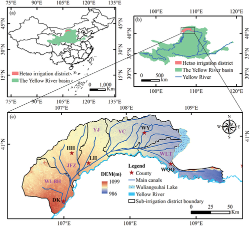
The study area used for mapping cropping systems in SF regions is the HID, the largest irrigation district in the arid region of Northwest China (Wen, Wan, and Shang 2023). The HID covers an area of about 12,000 km² in the northern part of the Yellow River Basin, featuring relatively flat topography and elevation ranging from 986 to 1,099 m (Figure 1). The HID aligns well with the purpose of this study, given that it is characterized by smallholder agriculture with diverse cropping patterns, complex crop types, fragmented cropland interspersed among other land cover types, and significant differences in cropping systems across different sub-irrigation districts.

Figure 1. Locations of the Yellow River basin in China (a), the Hetao Irrigation District (HID) in the Yellow River basin (b), and digital elevation model (DEM) of the HID (c). WLBH, JFZ, YJ, YC, and WLT represent the Wulanbuhe, Jiefangzha, Yongji, Yichang, and Wulate sub-irrigation districts, and DK, HH, LH, WY, and WQQ represent the Dengkou, Hangjinhouqi, Linhe, Wuyuan, and Wulateqianqi counties, respectively.

The HID’s climate is characterized as temperate continental arid and semi-arid environment (G. Li et al. 2022). The district encompasses diverse land use types, including lakes, deserts, wastelands, grasslands, croplands, and impervious surfaces (Wan, Qi, and Shang 2023), with cropland accounting for approximately 64% of the total area. Some of the cultivated areas have been farmed for a significant period and contribute to HID’s recognition as a World Heritage Irrigation Structure. In contrast, certain areas are at risk of soil salinization and unsuitable for farming. On average, each farm processes 1.1 ha of cropland (http://www.stats.gov.cn/sj/), and field survey results indicate that the typical size of the cropland is mainly in the range of 0.04–0.30 ha. The cropping patterns in HID include single cropping, double cropping, intercropping, cultivation-fallow, multiple harvest, and other minor patterns. Single cropping is the predominant pattern that includes sunflower, corn, seed zucchini, pepper, cherry tomato, and other crop varieties. Based on available studies and local surveys, the crops in HID have been gradually diversifying. In addition to the traditional staple crops of sunflowers, corn, and wheat, seed zucchini has emerged as another important crop in recent years. Additionally, minor crops have expanded from melons to chili peppers, cherry tomatoes, bell peppers, and onions, among others.

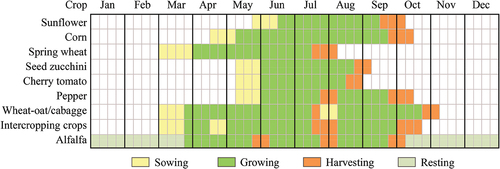
According to the Bureau of Agriculture and Animal Husbandry of Bayannur (http://nmj.bynr.gov.cn/) and field surveys, the crop calendar in HID is depicted in Figure 2. The earliest planted is usually spring wheat, typically sown in March. If intercropping with other crops such as corn or sunflower is intended, these intercropped crops are generally sown at the end of April, which are earlier than the usual crops. Crops in the second growing season, like oats or cabbage, are planted immediately after the wheat harvest to ensure sufficient growing time before soil freezing. Planting times for all crops may vary in different years due to climate conditions, which can present challenges in crop classification over multiple years (Hu et al. 2022).

Figure 2. Typical crop calendar in HID.

3. Data and methods

3.1 Reference data

The quantities of sample points, both visual interpreted samples and field samples, are displayed in Table 1. We conducted two surveys in HID, one from 27 September to 3 October 2020, and the other from 27 September to 7 October 2021. These surveys resulted in a total of 110,489 sample points in 2020 and 141,856 in 2021. The samples covered various cropping patterns, as well as prevalent crops such as sunflowers, corn, oats, seed zucchini, cherry tomatoes, bell peppers, and chili peppers. Due to the limited area of the wheat‒cabbage pattern, it was merged into the wheat‒oat pattern. Crops like cherry tomatoes, bell peppers, and chili peppers were classified as vegetables. Samples for 2018 and 2019 were carefully selected from visual interpretations, leveraging knowledge from field surveys and available high spatial resolution satellite images of Gaofen1 (2 m), Gaofen2 (1 m), and Google Earth (0.31 m) during the growing season. The reference image of characteristics for each crop are shown in Table S1. The crop types extractable through visual interpretation are limited, among which sunflowers, corn, seed zucchini, and vegetable samples are relatively easy to extract based on mono-temporal remotely sensed images. However, the sample size for wheat and alfalfa was 0 due to the difficulty of extraction by visual interpretation.

Table 1. Overview of visual interpreted samples (2018, 2019) and field collected samples (2020, 2021).

Year	Sunflower	Corn	Seed zucchini	Wheat-oat	Wheat-fallow	Vegetables	Intercropping	Alfalfa
2018	3,350	4,319	3,729	0	0	5,649	6,080	0
2019	22,929	21,209	19,031	0	0	6,352	0	0
2020	34,846	12,008	6,215	4,828	2,902	6,343	6,157	38,190
2021	45,714	42,089	19,882	6,862	5,568	8,663	9,810	3,268

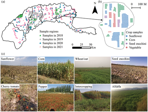
The field samples serve for both model training and validation, whereas the visual interpreted samples are used solely for model validation. Figure 3(a) depicts the overall distribution of the samples, with each point symbolizing a sampling region. Meanwhile, Figure 3(b) illustrates the detailed distribution of sample points within a specific sampling region. Figure 3(c) displays photos taken from different crop samples. The spacing between each sample point is 10 m. The field samples are distributed more evenly across the study area, while the visual interpreted samples are dispersed in limited regions covered by high spatial resolution images.

Figure 3. Spatial distribution of sampling regions in HID (2018–2021) (a), illustration of crop sample points in a sampling region (b), and photos of diverse crop samples (c).

The Ministry of Natural Resources of the People’s Republic of China, along with other relevant departments, conducted the third national land survey in China. This survey resulted in data regarding the cropland area at county level from 2019 to 2021 (https://gtdc.mnr.gov.cn/shareportal#/special/dataresources). Three counties, Hangjinhouqi, Linhe, and Wuyuan, are entirely encompassed in HID. As such, the cropland area of these three counties from 2019 to 2021 was also used as validation data for the extraction of croplands.

3.2 Creating the pool of feature variables

3.2.1 Sentinel-2 images and pre-processing

The S2 satellite system is comprised of two satellites, Sentinel-2A (launched on 23 June 2015) and Sentinel-2B (launched on 7 March 2017). The S2 satellite has a high spatial resolution of 10 or 20 m for the majority of the bands. The revisit time of the S2 system is 5 days at the equator after 7 March 2017, and has been reduced to 2–3 days in some parts of the mid-latitude regions (X. Chen et al. 2021). The temporal range of the S2 data used in this study spans from 1 January 2018 to 31 December 2021. The entire HID is covered by seven S2 scenes, where this study used 715 S2 images (ranging from 55 to 110 for each scene) each year to map the cropping systems. Consequently, an amount of 2,560 S2 images from 2018 to 2021 were used in the study.

In the years before 2019, only L1C data, the top of atmosphere (TOA) reflectance not atmospherically corrected, are available for use in GEE. In general, surface reflectance data are preferred, but several studies (Huang et al. 2022; Phalke et al. 2020; Wuyun et al. 2022) indicated that atmospheric correction for S2 in GEE is not necessary for classification when there is no complex spectral analysis. Therefore, this study uses TOA reflectance (S2 L1C) for classification over more periods and regions.

The preprocessing for S2 involves only cloud removal, as other steps such as radiometric calibration and geometric correction are already performed within the L1C product. More details about the cloud removal and other procedures for mapping cropping systems are available at https://code.earthengine.google.com/?accept_repo=users/qihongwei123321/Cropping_systems_S2. The QA60 band of S2 is widely used to remove opaque and cirrus clouds. However, identifying thin and semi-transparent clouds with QA60 presents a challenge (Zhu, Wang, and Woodcock 2015). To address this, we adopted Schmitt’s algorithm (Schmitt et al. 2019) and calculated the cloud score by assuming that all clouds are bright and humid. QA60, B1-B4, B8, B8A, B10, and B11 bands were used to detect clouds. The cloud detection results indicated that cloud coverage in the study area during the growing season is 27%, and the probability of a pixel being affected by clouds in 1 year is 34%. In areas where the image density is low, clear observations can be obtained every 8 days after removing clouds. The average spectral bands (red, green, blue, NIR (near-infrared), SWIR (short-wave infrared), and red edge) of the growing and non-growing seasons after the cloud removal are added to the pool of feature variables.

3.2.2 Construction of vegetation index time series

Different VIs represent and distinguish different features of crops. To compare the effect of different indices, we calculated the VIs commonly used for mapping cropping systems, and a total of 15 VIs were selected (Table 2). VIs calculated after removing the clouds cannot be directly used as feature variables because they are not uniform in time. The creation of equidistant, dense, and intra-annual composite time series of VIs is a commonly used approach for transforming the original VIs into data that can be used for classification purposes. We first generated the complete time series using linear interpolation and then used the Savitzky‒Golay (SG) filter to correct the anomalies (J. Chen et al. 2004). An appropriate interval of the time series can balance the data quality and help in distinguishing different features. The selection of temporal interval is related to the revisit period of the satellite, the coverage of the image, the probability of clouds, and the quality of the satellite images. The revisit time and the coverage of image are determined by the satellite and the location of the study region, respectively. In this study, we investigated the optimal time interval that balances both spectral heterogeneity and temporal continuity. We calculated the probability of time-series completeness after SG filtering using different time intervals to reveal the apparent lack of data when the time interval is shorter than 10 days. In the case of time intervals greater than 10 days, the data deviate significantly from the original data. Therefore, a comprehensive evaluation indicates that a time interval of 10 days is optimal. The window length of the SG filter and order of the filter is set to 3 as it is an optimal value for the crop growth curve (You et al. 2021).

Table 2. Vegetation indices used in mapping the cropping systems.

Vegetation index	Formula	Sentinel-2 bands	Reference
Normalized Difference Vegetation Index (NDVI)	(NIR–Red)/(NIR+Red)	(B8–B4)/(B8+B4)	(Rouse et al. 1976)
Normalized Difference Water Index (NDWI)	(Green–NIR)/(Green+NIR)	(B3–B8)/(B3+B8)	(McFeeters 1996)
Land Surface Water Index (LSWI)	(NIR–SWIR1)/(NIR+SWIR1)	(B8–B11)/(B8+B11)	(Xiao et al. 2005)
Normalized Difference Tillage Index (NDTI)	(SWIR1–SWIR2)/(SWIR1+SWIR2)	(B11–B12)/(B11+B12)	(Van Deventer et al. 1997)
Modified Normalized Difference Water Index (MNDWI)	(Green–SWIR1)/(Green+SWIR1)	(B3–B11)/(B3+B11)	(Xu 2006)
Red Edge Normalized Difference Vegetation Index (RENDVI)	(NIR–RE2)/(NIR+RE2)	(B8–B6)/(B8+B6)	(Gitelson and Merzlyak 1994)
Normalized Pigment Chlorophyll ratio Index (NPCI)	(Red–Green)/(Red+Green)	(B4–B3)/(B4+B3)	(Peñuelas et al. 1993)
Normalized Burn Ratio (NBR)	(NIR–SWIR2)/(NIR+SWIR2)	(B8–B12)/(B8+B12)	(García and Caselles 1991)
Plant Pigment Ratio (PPR)	(Green–Blue)/(Green+Blue)	(B3–B2)/(B3+B2)	(Metternicht 2003)
Normalized Difference Senescent Vegetation Index (NDSVI)	(SWIR1–Red)/(SWIR1+Red)	(B11–B4)/(B11+B4)	(Qi et al. 2002)
Modified NDVI (MNDVI)	(NIR–Red)/(NIR+Red–2*Aerosols)	(B8–B4)/(B8+B4–2*B1)	(Sims and Gamon 2002)
Enhanced Vegetation Index (EVI)	2.5*(NIR–Red)/(NIR+6*Red–7.5*Blue+1)	2.5*(B8–B4)/(B8+6*B4–7.5*B2+1)	(Huete et al. 1995)
Ratio Vegetation Index (RVI)	NIR/Red	B8/B4	(Tubaña et al. 2011)
Soil Adjusted Vegetation Index (SAVI)	1.428*(NIR–Red)/(NIR+Red+0.428)	1.428*(B8–B4)/(B8+B4+0.428)	(Huete 1988)
Red Edge Position index (REP)	700+40*((Red+RE3)/2)/(RE2–RE1)	700+40*((B4+B7)/2)/(B6–B5)	(Cho et al. 2007)

The period of the VI time series spanned from April to October annually, encompassing 91–301 days of the year (DOY), with one value attributed to each VI every 10 days, resulting in a total of 22 × 15 = 330 features that are added to the pool of feature variables. Figure S1 shows the time series of 15 VIs for four main single crops in HID. There are similarities and differences between different VIs, which means that each VI can help in the classification. In addition to the time series of VIs, we also performed a statistical analysis, including the three quartiles as well as the maximum and minimum values for selected VIs, and obtained a total of 75 features from the statistical analysis that were added to the pool of feature variables.

3.2.3 Calculation of phenology indices

The phenology index (PI) is used to describe the growth and developmental stages of crops, which is observed and recorded and then transformed into a numerical index. We used seven PIs based on the filtered NDVI time series to characterize crop phenology (Figure 4). These PIs include start of the season (SoS), end of the season (EoS), length of the season (LoS), fast growth phase (FGP), peak of the season (PoS), number of peaks (NoP), and fast growth speed (FGS).

Figure 4. A schematic diagram illustrating the retrieval of phenology indices for single (a) and double (b) crops using the threshold method.

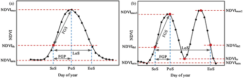
We used the threshold method (Descals et al. 2021) to determine the SoS and EoS as shown in Figure 4. The threshold of NDVI denoted by, NDVI_th, is calculated using the following equation:

(1) $\mathrm{NDV}{\mathrm{I}}_{\mathrm{th}}=(\mathrm{NDV}{\mathrm{I}}_{\max }-\mathrm{NDV}{\mathrm{I}}_{\min })\times \mathit{r}+\mathrm{NDV}{\mathrm{I}}_{\min }$(1)

where NDVI_max is the maximum NDVI, NDVI_min is the NDVI of bare croplands that is set as the mean NDVI from January to March, and the coefficient r is set to 0.3.

SoS is defined as the time when NDVI first exceeds the threshold (NDVI_th), and EOS is the first day in the late growing period when NDVI is smaller than NDVI_th. LoS is defined as the difference between EoS and SoS, whereas PoS is set to the time when NDVI reaches its peak. NoP represents the number of peaks in the NDVI time series and has an important role in understanding the cropping patterns. FGP and FGS are calculated from Eq. 2.

(2) $\mathrm{FGS}=\left(\mathrm{NDV}{\mathrm{I}}_{\max }-\mathrm{NDV}{\mathrm{I}}_{\mathrm{th}}\right)/\mathrm{FGP},\mathrm{FGP}=\mathrm{PoS}-\mathrm{SoS}$(2)

PoS is considered as the first peak of the curve when the curve has two or more peaks. The threshold for calculating the SoS is computed from the first peak, while the threshold for calculating the EoS is computed from the last peak of the curve. Finally, 7 PI features are added to the pool of feature variables.

3.3 Workflow for mapping the cropping systems

The workflow for mapping the cropping system is shown in Figure 5, where all steps are completed in GEE (https://code.earthengine.google.com/?accept_repo=users/qihongwei123321/Cropping_systems_S2). Three components of the cropping systems, including cropland, cropping pattern, and crop types are considered in the workflow. The major steps are comprised of generation of feature variable datasets and reference datasets, extraction of cropland, classification of cropping patterns and crop types, and evaluation of the results.

Figure 5. Workflow for mapping cropping systems. OCSVM in the workflow refers to one-class support vector machine.

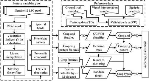
3.3.1 Cropland extraction

In the process of cropland extraction, this study utilized a one-class classifier that allows for the extraction of croplands without the need for samples of other land use/land cover types, thereby reducing the effort required for labeling non-cropland samples. The one-class support vector machine (Schölkopf et al. 2001, OCSVM) has been successfully used in land-cover or crop classification using satellite imagery (Lei et al. 2021; Yang et al. 2021), where a non-linear kernel was used to map the data into a higher-dimensional space, allowing for the separation of specific category from other categories. Therefore, this study used OCSVM to map the cropland. It is noteworthy that cropland is mapped annually to detect the newly cultivated and abandoned cropland in SF regions. This iterative process constitutes a crucial component in monitoring agricultural practices.

Cropland is a collection of all types of artificially planted crops. According to field survey results, the relatively important features of artificially planted crops are the presence of bare soil and dense vegetation. These features can be reflected by the statistical variables of VI represented by NDVI, and spectral bands (red, green, blue, NIR, SWIR, red edge) in both growing and non-growing seasons. In addition, some croplands also plant alfalfa in HID, which do not have the status of bare soil and can be reflected by phenological variables such as NoP and LoS to distinguish them from other natural grasslands. Therefore, the feature variables used for cropland extraction mainly include phenological variables, statistical variables of NDVI, and spectral band variables.

The dataset used for training the OCSVM consisted of cropland field samples in 2020, with 1,000 training points for each crop, resulting in a total of 8,000 training samples. Two hyperparameters, Nu and Gamma of the Gaussian kernel, are calibrated with the statistical cropland area at the county level in 2019. The validation process included statistical cropland area in 2020 and 2021, along with cropland field samples from 2018 to 2021. The calibration results (as shown in Table S2 in the supplementary material) revealed that Nu significantly influenced the accuracy of cropland extraction; however, Gamma has no significant impact. The calibrated Nu was 0.06 corresponding to the highest overall precision (Table S2), and Gamma was 0.05.

3.3.2 Cropping pattern classification

The cropping pattern refers to the number, order, and spatial interval of crop types cultivated on a piece of arable land in 1 year. Specifically, single cropping refers to the cultivation of a single crop on a piece of arable land in 1 year. Intercropping refers to the cultivation of two crops being planted with cross-distribution in 1 year on a piece of arable land. Double cropping refers to the practice of cultivating one crop after another on a piece of arable land, where the second crop is planted after the harvest of the first crop. Cultivation-fallow is the practice of planting crops in the first growing season; however, no other crops are planted in the second growing season. Another special planting type is alfalfa, which generally refers to perennial crops that are harvested repeatedly each year and is mainly called multiple harvest.

Figure 6 shows the NDVI curves of different cropping patterns and crops. Different cropping patterns exhibit different characteristics during the sowing, growth, and harvesting stages. For example, the NDVI curve of the multiple harvest pattern (alfalfa) has three or four peaks depending on the number of harvests in a single year. On the other hand, the wheat-fallow pattern has a small NDVI peak after wheat harvest due to the germination of wheat seeds left in some croplands despite the fallowing of the land. The intercropping pattern has different characteristics at different harvesting times, different crops planted, etc., with possible peak numbers of one or two. Therefore, cropping patterns other than multiple harvest patterns need to be classified by indicators such as EoS, LoS, the trough value of the NDVI curve (NDVI_tv), and the second peak value of the NDVI curve (NDVI_max2) (Figure 4). The specific decision tree rules for these cropping patterns are shown in Figure S2, where thresholds are estimated based on sample points in 2021.

Figure 6. NDVI time series curves for different cropping patterns and crop types. Solid lines are single cropping patterns, while dotted lines represent the other 4 cropping patterns.

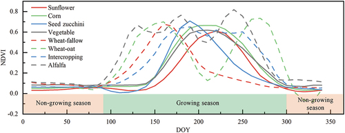
Since the areas of intercropping patterns are small, we do not have enough samples to distinguish different intercropping patterns. We used the K-means++ clustering (Arthur and Vassilvitskii 2007) method to classify the intercropping patterns, which is a widely used unsupervised classification method that can effectively solve the problem of small sample size, especially when the number of classes is small.

The difference in vegetation growth of different intercropping patterns is significant mainly in August–September. The feature variables used to distinguish different intercropping patterns mainly included NDVI and RENDVI in August–September. The number of clusters is essential for clustering. According to our field survey, the intercropping types in HID are mainly wheat/sunflower, wheat/corn, wheat/zucchini, etc., but the wheat/sunflower and wheat/corn cropping patterns are dominant. Additionally, we used the elbow method (Syakur et al. 2018) to find the best number of clusters. The results (shown in Fig. S3) also showed that the appropriate number of clusters was 2, which also agreed with the results from field surveys.

3.3.3 Crop classification

Based on the classification results of the cropping pattern, specific crops are classified including sunflower, corn, wheat, seed zucchini, vegetables, and alfalfa. The classification results of the cropping pattern contribute to the classification of crops. Field surveys have revealed that the single cropping pattern involves a diverse range of crops, such as sunflower, corn, and seed zucchini, among others. Double cropping and intercropping patterns primarily revolve around the growth of wheat. Double cropping entails sowing oats after the wheat harvest in summer, while intercropping comprises the cultivation of wheat with either corn or sunflower. The multiple harvest pattern solely involves alfalfa cultivation in HID. Notably, crop classification is simple for all patterns except single cropping; therefore, our study focused on identifying single crops (e.g. sunflower, corn, seed zucchini, and vegetables) in single cropping pattern. RF classifier is used in this study to classify crops in single cropping pattern.

The RF classifier (Breiman 2001) is less sensitive to data noise (Teluguntla et al. 2018), which mitigates the effect of noise from the TOA data. Moreover, the RF classifier is well-suited for large quantities of input variables since they are unaffected by collinearity and redundancy among the features. However, training datasets with all 405 features exceeded the user limit in GEE platform and feature selection is necessary. The limitation of training datasets in GEE is usually determined by the arithmetic capability of noncommercial users and the algorithm used. Generally, datasets in RF are limited to n×b ≈ 5,000,000, where n is the number of samples and b is the number of features that should be less than 400. A proper ratio of b to n is approximately 20 to 50 (Van Der Ploeg, Austin, and Steyerberg 2014). Therefore, we carefully set our dataset by selecting 6,000 samples per class with approximately 150 features to achieve a ratio of approximately 40.

It should be noted that 150 features need to be selected out of 405 feature variables. Several studies have employed variable importance to simplify the model by eliminating variables with low importance in GEE (Belgiu and Drăgu 2016), which is a typical approach for feature variable selection. However, it is a challenge to run the RF classifier first in GEE to get the variable importance results for a large dataset. In addition, feature selection based on the variable importance was influenced by the correlation between variables (Gregorutti, Michel, and Saint-Pierre 2017). However, the correlation between some variables is strong because all the variables are associated with vegetation growth status. Therefore, we used the Jeffries-Matusita distance (JMD) for feature selection (Dabboor et al. 2014), which serves as a measure of feature ranking for binary classification problems and requires limited computing resources (Sen, Goswami, and Chakraborty 2019). The JMD between two classes is given by

(3) $\mathrm{JMD}(\mathit{i},\mathit{j},\mathit{k})=\sqrt{2\left(1-\int \sqrt{\mathit{p}(x_{\mathit{i},\mathit{k}})\mathit{q}(x_{\mathit{j},\mathit{k}})}\mathrm{d}\mathit{x}\right)}$(3)

where p(x_i,k) and p(x_j,k) are the probability distribution functions of feature variable k for crop i and crop j, respectively.

We ranked the JMD and selected three vegetation indices of each binary crop classification with the largest JMD (Table S3). Six of the best vegetation indices (REP, PPR, RENDVI, NDTI, MNDWI, and NPCI) are selected to classify different crops. The time series and statistical values of the above six indices are finally identified as features used in crop classification.

The training samples for RF consist of sampling points in 2020 and 2021, with 3,000 points per crop category (i.e. sunflower, corn, seed zucchini, and vegetables) per year (2020 and 2021). The use of training dataset from 2 years facilitated the construction of a more robust and generalized classifier that considers the variation in vegetation growth under different conditions of climate, soil and water management (Massey et al. 2017). This increased stability is valuable when applying the classifier to multiple years, as it enhances the classifier’s ability to handle diverse conditions effectively. The validation samples consist of crop samples collected for the period 4 years, i.e. from 2018 to 2021.

Two hyperparameters of RF (numberOfTrees and variablesPerSplit) are generally subject to tuning (Belgiu and Drăgu 2016). For the optimization of the numberOfTrees, we employed internal testing (Fig. S4) and the results indicated that an optimal accuracy is achieved with 150. On the other hand, the variablesPerSplit (“Mtry” for RF in R programming language) was set to the default value, which is the square root of the total number of variables. Other parameters of the RF, such as node size and depth, took their default settings.

3.3.4 Accuracy assessment

The classification accuracy was evaluated from two aspects, i.e. area accuracy and the sampling point accuracy, using the following accuracy indicators:

(4) $\mathrm{RE}=\left(\mathrm{Are}{\mathrm{a}}_{\mathrm{identified}}-\mathrm{Are}{\mathrm{a}}_{\mathrm{statistical}}\right)\times \mathrm{Are}{\mathrm{a}}_{\mathrm{statistical}}\times 100\mathrm{\%}$(4)

(5) $\mathrm{OA}={\sum }_{\mathit{i}=1}^n\left(\mathrm{T}{\mathrm{P}}_i+\mathrm{T}{\mathrm{N}}_i\right)/\left(\mathrm{T}{\mathrm{P}}_i+\mathrm{T}{\mathrm{N}}_i+\mathrm{F}{\mathrm{P}}_i+\mathrm{F}{\mathrm{N}}_i\right)$(5)

(6) $P_i=\mathrm{T}{\mathrm{P}}_i/\left(\mathrm{T}{\mathrm{P}}_i+\mathrm{F}{\mathrm{P}}_i\right)$(6)

(7) $R_i=\mathrm{T}{\mathrm{P}}_i/\left(\mathrm{T}{\mathrm{P}}_i+\mathrm{F}{\mathrm{N}}_i\right)$(7)

(8) $\mathrm{F}{1}_i=2P_i\times R_i/\left(P_i+R_i\right)$(8)

(9) $\mathrm{Io}{\mathrm{U}}_i=\mathrm{T}{\mathrm{P}}_i/\left(\mathrm{T}{\mathrm{P}}_i+\mathrm{F}{\mathrm{P}}_i+\mathrm{F}{\mathrm{N}}_i\right)$(9)

(10) $\mathrm{mIoU}={\sum }_{\mathit{i}=1}^n\mathrm{Io}{\mathrm{U}}_i/\mathit{n}$(10)

where RE, OA, P_i, R_i, F1_i, IOU_i, and mIOU are the relative error, overall accuracy, precision, recall, F1-score, intersection-over-union, and mean IoU, respectively; i is the number of the n categories of crops; TP (true-positive), FP (false-positive), and FN (false-negative) are combinations of different cases of classification results and sample actual results. TP and FP represent the results of correct classification and misprediction the positive class. In contrast, FP and FN represent the results of incorrectly classification and prediction the negative class, respectively. Area_identified and Area_statistical represent the area of identified elements and the official statistical area with the same element, respectively.

Area accuracy was assessed using the RE between the extracted and statistical areas (Equation 4(4) $\mathrm{RE}=\left(\mathrm{Are}{\mathrm{a}}_{\mathrm{identified}}-\mathrm{Are}{\mathrm{a}}_{\mathrm{statistical}}\right)\times \mathrm{Are}{\mathrm{a}}_{\mathrm{statistical}}\times 100\mathrm{\%}$(4) ). Sampling point accuracy was used for the extraction of cropland, classification of cropping patterns, and crop classification using OA, P, R, F1, IoU, and mIoU (Equation 5(5) $\mathrm{OA}={\sum }_{\mathit{i}=1}^n\left(\mathrm{T}{\mathrm{P}}_i+\mathrm{T}{\mathrm{N}}_i\right)/\left(\mathrm{T}{\mathrm{P}}_i+\mathrm{T}{\mathrm{N}}_i+\mathrm{F}{\mathrm{P}}_i+\mathrm{F}{\mathrm{N}}_i\right)$(5) -10(10) $\mathrm{mIoU}={\sum }_{\mathit{i}=1}^n\mathrm{Io}{\mathrm{U}}_i/\mathit{n}$(10) ). Choosing different accuracy indicators helps to understand different aspects of model performances (G. Li et al. 2022).

To ensure the consistency of indicators used in the calculation of classification accuracy in different years, the numbers of validation points of different classes are set to the same value. The validation points of cropland extraction are set to 1,000 for each crop, while the validation points of cropping pattern classification and crop classification are set to 2,500 for each cropping pattern and 3,000 for each single crop. The process of randomly selecting samples for accuracy evaluation was repeated 10 times and their average value was taken as the accuracy of the validation.

4. Results

4.1 Accuracy assessment of the proposed workflow in mapping cropping systems

The accuracy assessment results of cropland extraction (Table 3), cropping pattern classification (Table 4), and crop classification (Table 5) show the high accuracy of the proposed workflow.

Table 3. Comparisons of statistical and extracted cropland areas in the county level.

	Statistical area (km^2)			Extracted area (km^2)				Relative error (RE)
County	2019	2020	2021	2018	2019	2020	2021	2019	2020	2021
Wuyuan	1,699	1,702	1,707	1,670	1,609	1,676	1,518	−5.3%	−1.5%	−11.1%
Linhe	1,550	1,546	1,550	1,609	1,610	1,679	1,664	3.9%	8.6%	7.4%
Hangjinhouqi	1,099	1,099	1,104	1,162	1,134	1,187	1,170	3.2%	8.0%	6.0%
Total of 3 counties	4,348	4,347	4,361	4,441	4,352	4,542	4,351	0.1%	4.5%	−0.2%

Table 4. The accuracy of cropping pattern classification.

Year	Accuracy	Single cropping	Double cropping	Intercropping	Multiple harvest	Wheat-fallow	mIoU	OA
2020	R	0.960	0.994	0.958	0.999	0.905
	P	0.939	0.961	0.943	0.995	0.987
	F1	0.949	0.977	0.950	0.997	0.944
	IoU	0.904	0.955	0.906	0.994	0.894	0.931	0.962
2021	R	0.983	0.981	0.937	0.949	0.956
	P	0.925	0.988	0.958	0.996	0.958
	F1	0.953	0.984	0.947	0.972	0.957
	IoU	0.910	0.969	0.900	0.945	0.918	0.929	0.962

Table 5. The accuracy of crop classification. NA refers to not available.

Year	Accuracy	Sunflower	Corn	Seed zucchini	Vegetables	Wheat	Alfalfa	mIoU	OA
2018	R	0.976	0.999	0.961	0.874	NA	NA
	P	0.992	0.966	0.943	0.973	NA	NA
	F1	0.984	0.982	0.952	0.921	NA	NA
	IoU	0.968	0.965	0.908	0.853	NA	NA	0.924	0.951
2019	R	0.992	0.997	0.985	0.933	NA	NA
	P	0.993	0.994	0.945	0.999	NA	NA
	F1	0.992	0.995	0.965	0.965	NA	NA
	IoU	0.985	0.991	0.932	0.932	NA	NA	0.960	0.978
2020	R	0.991	0.988	0.973	0.988	0.981	0.999
	P	0.985	0.995	0.980	0.992	0.973	0.996
	F1	0.988	0.991	0.976	0.990	0.977	0.998
	IoU	0.976	0.983	0.854	0.980	0.955	0.996	0.974	0.987
2021	R	0.985	0.976	0.993	0.988	0.969	0.966
	P	0.990	0.949	0.998	0.963	0.977	0.999
	F1	0.987	0.962	0.995	0.975	0.956	0.982
	IoU	0.975	0.927	0.991	0.952	0.968	0.965	0.961	0.980

From Table 3, the extracted cropland area in the three counties matched the statistical area well, with the maximum absolute RE of around 11% in the county level and less than 5% in the total cropland area in the three counties. Moreover, the OA values of the cropland validation points from 2018 to 2021, 0.99, 0.99, 0.97, and 0.95, were notably high. These comparisons demonstrated the effectiveness of OCSVM for cropland extraction with only crop samples. The model performed well in extracting cropland information from the complex land use/land cover after its training and calibration, thereby saving great efforts in collect samples of other types of land use/land cover.

The accuracy of the cropping pattern classification was high (Table 4), with OA values of 0.962 in both 2020 and 2021. The corresponding mIoU values for the same years are 0.931 and 0.929, respectively. The R is significantly higher than the P for single cropping in 2020 and 2021, indicating that single crops are extracted perfectly. However, other types of crops are classified as single crops and the area extracted will be slightly higher than the actual area. In contrast, wheat-fallow, and multiple harvest patterns had higher P than R in 2020 or 2021, indicating that these two types of cropping patterns were slightly misclassified and some samples were missed. The R and P are closer to F1 for double cropping and intercropping patterns, which are either misclassified or missed. Although there are some problems with misclassification or omission in some categories, but the results shown high R and p values. The IoU and F1 results similarly demonstrate that our method is effective in classifying four cropping patterns.

Table 5 indicates high accuracy for crop classification, with the OA ranging from 0.951 to 0.987 and mIoU from 0.924 to 0.974. The accuracy in 2018 was slightly lower as compared with other 3 years; however, the results were still reliable with OA and mIoU of 0.951 and 0.924, respectively. The results of P, R, F1, and IoU show that the accuracy of different crops is significantly different, among which the accuracies is highest for sunflower and alfalfa, and lowest for vegetables. The results show that all accuracy indicators are higher for sunflower and alfalfa, where the IoU values are all above 0.965 during the study period of 4 years, indicating that sunflower and alfalfa are perfectly extracted. The R of vegetables is significantly lower than P and resulted in lower F1 and IoU, which indicates that some vegetable samples were classified as other samples. The main reason of this misclassification lies in the fact that, vegetables are a collection of several crop types having different characteristics, which results in the relatively poor classification accuracy.

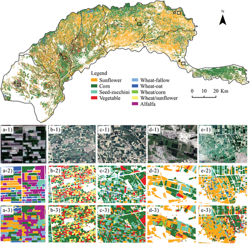
Figure 7 shows the distribution of the cropping system in HID in 2021, where the comparison is also performed with high spatial resolution satellite imageries across five distinct areas in HID. It is evident from the figure that there is a high level of similarity between the cropping system and the visual interpretation maps in space. Figures 7(a–1–e–1) demonstrate that the workflow has successfully extracted the cropland, while excluding villages, wasteland, and roads. The crop maps that include various types of crops are also consistent with the reference maps. From the details of the classification results, the method produced highly aggregated outputs, with the boundaries between the different crop types appearing very tidy. The spatial resolution of S2 is also well-suited for mapping cropping systems in HID. A major limitation of the classification results is that some small patches within the cropland and non-cropland are identified into the wrong categories, which may possibly be the drawback of pixel-scale classification. Although the results display distinct field features at pixel scale, the examination of crop distribution results illustrates that the classification is trustworthy, and the workflow is robust enough to map the cropping system accurately.

Figure 7. Spatial distributions of the cropland, cropping patterns, and crop types in 2019 in HID, where the white represents non-cropland areas. The zoomed-in views for the five regions (coordinates are given in Table S4) are shown in Figures 7 a-3) to e-3) And the high spatial resolution views from Google Earth or Gaofen satellites are shown in Figures 7 a-1) to e-1). The reference crops map by visual interpretation for five regions are shown in Figures 7 a-2) to e-2). The gray color parts in Figures 7 a-2) to e-2) indicates that the category cannot be determined by visual interpretation. The process of creating a-2) using six images is shown in Figure S5.

4.2 Distribution of cropping systems in HID

The distributions of the cropland, cropping pattern, and crop types are shown in Figure 8. In general, the croplands in HID are mainly distributed in the middle and eastern parts. The croplands in the western HID are concentrated in several regions surrounded by desert. The single cropping pattern is the dominant cropping pattern of HID, accounting for 89.42% of the cropland. The double cropping, intercropping, wheat-fallow, and multiple harvest patterns are distributed in all sub-irrigation districts; however, their proportion is dominant in the west of HID as compared with that in the east of HID.

Figure 8. The distributions of cropland, cropping patterns and crop types in 2018 (a), 2019 (b), 2020 (c), and 2021 (d). WLBH, JFZ, YJ, YC, and WLT represent the Wulanbuhe, Jiefangzha, Yongji, Yichang, and Wulate sub-irrigation districts, respectively. The white represents non-cropland areas. The relationships between crop types and cropping patterns are shown in the bottom of Figure 8.

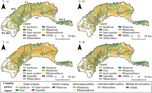
The crop distribution maps show that sunflower and corn are the most commonly planted crops in HID, and are widely distributed throughout the entire HID. Sunflower is relatively concentrated in the central and eastern parts of the HID. Wen, Shang, and Ur Rahman (2019) and G. Li et al. (2023) also indicated that sunflower is mainly distributed in YC, and this spatial distribution is mainly associated with the distribution of soil salinity as sunflower is more salt-tolerant than other crops. On the other hand, corn is mainly distributed in the western and eastern parts of the HID. Crops other than corn and sunflower have relatively poor salt-tolerant and thus require better quality of cropland, and therefore are scattered in different areas. Seed zucchini and vegetables are mainly distributed in the eastern part of the HID, whereas wheat-fallow, wheat-oat, wheat/sunflower, and wheat/maize are mainly concentrated in the JFZ and YJ sub-irrigation districts. Further, alfalfa is mainly concentrated in the WLBH sub-irrigation district.

4.3 Temporal variations in cropping systems in HID

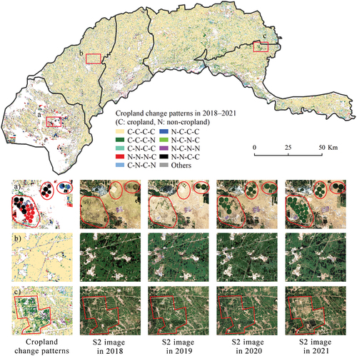
The variation in cropland change patterns from 2018 to 2021 is shown in Figure 9, which integrated the results of four-year cropland extraction. Each pixel has two states per year, i.e. cropland or non-cropland. Overall, there are a total of 15 patterns in these years except the intersection of the non-cropland pattern for 4 years, which is shown as the white area in Figure 9. The main nine patterns are shown separately, whereas the remaining six minor patterns are classified as others (Figure 9). Because of the poorer environment for cropping and the desire for more arable croplands, the croplands in the western HID (region a in Figure 9) expanded gradually in regions convenient for reclamation. The croplands in the middle of HID (region b in Figure 9) extended in large areas, and villages are scattered among the croplands. Soil salinity is dominant in the eastern HID (Wen, Wan, and Shang 2023), which results in frequent conversion between cropland reclamation and abandonment and thus more cropland change patterns (region c in Figure 9). The annual changes in cropland area and their distribution highlighted the necessity of extracting cropland each year for precise crop classification. The various changes in croplands over the four-year study period also verified the accuracy and effectiveness of the method in mapping croplands.

Figure 9. Distributions of cropland change patterns in HID and their transformations during the peak growing season using sentinel-2 imagery over three typical regions (a, b, c) from 2018 to 2021. The status of cropland (represented by C) and non-cropland (denoted by N) areas during the four years (2018–2021) is shown with different combinations. For example, the combination of C-C-C-N represents that the pixel is cropland in 2018, 2019, and 2020, while non-cropland in 2021. The white areas represent non-cropland during all the four years.

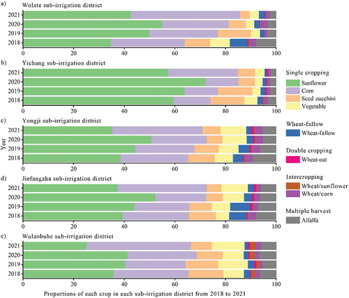
From the temporal changes in cropping patterns and crop types in each sub-irrigation district shown in Figure 10. The results show that single cropping pattern has an increasing trend from 1 year to another during the study period. It should be noted that the increasing trend of single cropping pattern is observed in all sub-irrigation districts except WLBH. This may be associated with the lower labor cost of single cropping. Due to the subsidy for double cropping pattern from the government, the proportion of double cropping has been significantly increased. The acreage of wheat (wheat-fallow, wheat-oat, wheat/maize, and wheat/sunflower) and seed zucchini is decreased by 35.20% and 46.14% from 2018 to 2021, respectively. The acreage of alfalfa is relatively stable, while that of vegetables is increased by 20.45%. In contrast, sunflower and corn depicted no clear trends over the years.

Figure 10. Proportions of each crop in sub-irrigation districts of Wulate (a), Yichang (b), Yongji (c), Jiefangzha (d), and Wulanbuhe (e) from 2018 to 2021.

5. Discussions

5.1 The necessity to update cropland mapping annually

The necessity to map cropland every year may depend on the local cropping situation. For SF regions where the situation is not much clear, annual cropland mapping can aid in determining whether the extent of the cropland is consistently changing. In instances where the changes in cropland distribution are minimal, it may be sufficient to map the cropland once several years. However, field surveys and available study (Zhao et al. 2021) showed that the cropland system is not stable in HID. Some regions showed continuous expansion of the cultivated lands through continuous reclamation, while others suffer from poor soil quality that hinders the process of consecutive cultivation and results in abandonment of the croplands (Csikós and Tóth 2023). The proportion of land recultivated (or newly reclaimed) and abandoned can be calculated from Figure 9. “C-N” represents cropland that has been abandoned, while “N-C” indicates that cropland that has been recultivated for farming. For example, the comparison of cultivated areas from 2018 to 2019 shows that recultivated and abandoned cropland areas in 2019 are 516 km² (6.50% of the total cultivated croplands) and 606 km² (7.64% of the total), respectively. Despite minor changes in total cropland area from 2018 to 2019, the sum of changed areas (i.e. cultivated or abandoned areas) accounts 14.14% of the total cropland. It is necessary to map the cropland each year to reflect the inter-annual changes in cropland.

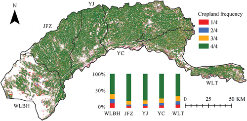
The frequency of each pixel classified as cropland in the 4 years is shown in Figure 11, where the bar chart shows the cumulative percentages of cropland frequencies in different sub-irrigation districts. The results show that the distribution of cropland in HID is not consistent over the 4 years. Generally, the middle areas of HID has high frequencies of cropland, while WLBH and WLT had low frequencies. Approximately 79% of the croplands in JFZ and YJ were cultivated continuously between 2018 and 2021. The proportion of areas with low frequencies of cropland is small in all sub-irrigation districts, indicating gradual changes in cropland areas, such as expansion and shrinkage. Based on the spatial distributions and changes in cropland areas within sub-irrigation districts, the low cropland frequency in WLBH may be mainly due to the expansion of new croplands. Furthermore, the low cultivation frequency in YC and WLT is mainly due to the fact that some cultivated croplands being unsuitable for continuous cultivation. In summary, annual mapping of cropland is instrumental in comprehending the cropping systems in SF regions.

Figure 11. Frequency of cropland occurrence per pixel from 2018 to 2021 and the proportions of different frequencies in the sub-irrigation districts. WLBH, JFZ, YJ, YC, and WLT represent the Wulanbuhe, Jiefangzha, Yongji, Yichang, and Wulate sub-irrigation districts, respectively.

5.2 Time-scale matching of S2 images to crop phenology

The phenology index calculated based on time-series curves is an important feature for extracting cropland information and classifying cropping patterns. It is very efficient and convenient to classify the cropping patterns based on the phenology index after the accurate calculation of vegetation index time-series curves. The accuracy of time-series curves to simulate phenological changes are dependent of the number of points used in computation of time-series curves and the spatial resolution of the pixels (Zeng et al. 2020).

S2, consisting of two satellites in the orbit, made it possible to comprehend the crop phenology under complex situations. We calculated the longest time interval (T) of S2, which represents the longest period of consecutive days without clear satellite images at a specified location in a year. The crop growth cannot be monitored well when T is too large. For example, the duration between two harvests of alfalfa is generally 30 days; therefore, the cropping patterns of alfalfa with multiple harvests cannot be identified if T >30 days. T of S2 is usually less than 20 days in most of the HID, which is applicable to phenology extraction. In contrast, the T value of Landsat-8 is between 16 and 112 days, which cannot be used to map the cropping system in HID.

The T determines how accurately the vegetation index simulates phenology. The knowledge of crop phenology and T is important to know in advance whether the satellite products used can meet the requirements. Overall, the results of this study demonstrated that S2 can be used to study cropping systems in similar SF regions as in HID.

5.3 The advantages and limitations of the workflow

The proposed workflow not only demonstrates satisfactory performance in mapping the cropping systems, but also introduces several advancements in comparison with existing studies. First, the workflow is centered around S2 having high spatial resolution that can reduce the severe mixed-pixel impact in SF regions. This unique focus on high-resolution imagery is a key differentiator from previous methods. Second, it covers cropland extraction, cropping pattern classification, and crop mapping, thereby offering more comprehensive information about cropping system. Third, this workflow is capable of annual cropland mapping, which can be used to detect both the reclamation and abandonment of cropland in SF regions and marks a significant improvement in dynamic land use monitoring. Fourth, the extraction of croplands requires only cropland samples, and thus saves the cost of collecting samples of other land use/land cover types. Fifth, the workflow uniquely utilizes phenological variables based on the time series of VIs calculated by S2 data to classify a wide range of cropping patterns, such as single cropping, double cropping, cultivation‒fallow, intercropping, and multiple harvest pattern, etc. This workflow can also be used to extract other cropping system in similar regions that are not covered in this paper, such as short-term rotation (e.g. corn‒soybean) and tri-cropping. When the period for cropping system mapping is longer, this framework can also be used to investigate long-term rotation (e.g. corn‒oat‒wheat‒soybean) as well as alternate cropland cultivation and fallowing. This extensive capability in crop pattern classification sets the study apart from others in the field. Last, conducting crop classification after the classification of cropping patterns reduces the false-positive rate of crop classification and enhances the credibility of the classification results. Moreover, the implementation of the entire workflow in GEE not only demonstrates its practical applicability, but also sets a new standard for simplicity and adaptability in cropping systems studies.

Although the method has achieved good results over the study years, there are still limitations that can be studied further. First, the framework is built on pixel-based classification, which can lead to misclassification at the boundaries of different types of croplands. For instance, the border area between a sunflower field and a corn field might be incorrectly classified as vegetables. High spatial resolution satellite imagery can effectively address this issue (Estes et al. 2022). However, obtaining such imagery can be challenging. In the absence of high-resolution imagery, it may be beneficial to employ methods such as spectral unmixing (Rauf et al. 2022) and object-based classification method (Peña-Barragán et al. 2011). Second, the workflow requires field crop samples for model training. In the absence of samples, it can only be used to distinguish between single, double, and multiple harvest patterns. Finally, this study only spans 4 years due to available S2 data and research time constraints. It is uncertain whether the change in cropland status is due to cropland fallowing management or stem from an abandonment due to poor soil quality. This workflow can be further explored for extracting the potential value of VI time series, such as using the dynamic time warping alignment (Gao et al. 2021) to reduce noise and enhance applicability over multiple years.

6. Conclusions

This study proposed a novel integrated workflow to map cropping systems by combining one-class support vector machine, unsupervised classification, decision tree, and RF algorithms, and explored the applicability of S2 data in mapping cropping systems in the HID of Northwest China characterized by smallholder farms. The following conclusions can be drawn from the study.

1. S2 data can be used to obtain information on cropland extent, cropping patterns, and crop types in the complex cropping systems of the SF regions. The cropping patterns at least involved single cropping, double cropping, intercropping, multiple harvest, and fallow patterns. The crop types considered in the study area include sunflower, corn, wheat, seed zucchini, alfalfa, and vegetables.

2. The workflow is simple, fast, and efficient with the free S2 data and computing resources provided by GEE. The results showed that accuracy in multiple years is high and reflected the robustness of the proposed approach. The results also highlighted that the complexity of agricultural activities in SF regions and the poor continuity of farming activities make it necessary to map the cropland and update it annually instead of using the existing land use/land cover products.

3. The innovative reliance on the simulating crop phenology time-series curves and calculating various phenological variables using S2 data represents a significant advancement in crop monitoring. The S2 data with a temporal resolution of 5 days are able to accurately identify changes in plant growth status over a time span of 20 days. This value is affected by cloud cover and latitude, which decreases with decreasing cloud cover and increasing latitude. REP, PPR, and RENDVI demonstrated high capabilities in classifying various types of crops.

4. The mapping results showed that the continuity of cropland cultivation in HID is poor and 26% of the farmland has different degrees of abandonment. The proportion of the single cropping pattern is increased from 1 year to another. Further, the results showed that proportion of the double cropping pattern is also increased significantly, which may be due to the subsidy provided by the government. The area of wheat is decreased significantly and farmers preferred to plant vegetables or corn, which are more likely to yield substantial economically returns. These findings have significant implications for understanding agricultural trends and policy impacts in the study region.

Although the proposed method is simple and effective, it requires crop samples. How to achieve accurate classification of cropping systems without field samples needs further investigation.

Acknowledgments

We would like to thank Dr. Khalil Ur Rahman from Tsinghua University for proofreading the manuscript. Additionally, we are thankful to the editors and anonymous reviewers, whose comments and suggestions are valuable for improving the manuscript.

Disclosure statement

No potential conflict of interest was reported by the author(s).

Data availability statement

The data that support the findings of this study are available from the corresponding author, S. Shang, upon reasonable request.

Supplementary material

Supplemental data for this article can be accessed online at https://doi.org/10.1080/15481603.2024.2309843

Additional information

Funding

This work was supported by the National Natural Science Foundation of China under Grant numbers 51839006 and 52279038.

References

- Arthur, D., and S. Vassilvitskii. 2007. “K-Means++: The Advantages of Careful Seeding.” Proceedings of the Annual ACM-SIAM Symposium on Discrete Algorithms, January 7-9, New Prleans, Louisiana, USA, 1027–23.
- Belgiu, M., and L. Drăgu. 2016. “Random Forest in Remote Sensing: A Review of Applications and Future Directions.” ISPRS Journal of Photogrammetry and Remote Sensing 114:24–31. https://doi.org/10.1016/j.isprsjprs.2016.01.011.
- Blanco-Canqui, H., and L. Rattan. 2008. “Cropping Systems BT - Principles of Soil Conservation and Management.” In, edited by H. Blanco-Canqui and R. Lal, 165–193. Dordrecht: Springer Netherlands. https://doi.org/10.1007/978-1-4020-8709-7_7.
- Borboudakis, G., and I. Tsamardinos. 2021. “Extending Greedy Feature Selection Algorithms to Multiple Solutions.” Data Mining and Knowledge Discovery 35: 1393–1434. https://doi.org/10.1007/s10618-020-00731-7.
- Boryan, C., Z. Yang, R. Mueller, and M. Craig. 2011. “Monitoring US Agriculture: The US Department of Agriculture, National Agricultural Statistics Service, Cropland Data Layer Program.” Geocarto International 26 (5): 341–358. https://doi.org/10.1080/10106049.2011.562309.
- Breiman, L. 2001. “Random Forests.” Machine Learning 45 (1): 5–32. https://doi.org/10.1023/A:1010933404324.
- Chen, X., P. An, K. Laakso, G. Arturo Sanchez-Azofeifa, F. Wang, G. Zhang, L. Jiang, et al. 2021. “Satellite-Based Observations of the Green Depressing Cropping System in a Farming-Pastoral Ecotone of Northern China.” International Journal of Applied Earth Observation and Geoinformation 98:102312. The Authors. https://doi.org/10.1016/j.jag.2021.102312
- Chen, J., P. Jönsson, M. Tamura, Z. Gu, B. Matsushita, and L. Eklundh. 2004. “A Simple Method for Reconstructing a High-Quality NDVI Time-Series Data Set Based on the Savitzky-Golay Filter.” Remote Sensing of Environment 91 (3–4): 332–344. https://doi.org/10.1016/j.rse.2004.03.014.
- Chen, Y., D. Lu, E. Moran, M. Batistella, L. V. Dutra, I. D. A. Sanches, R. F. B. da Silva, J. Huang, A. J. B. Luiz, and M. A. F. de Oliveira. 2018. “Mapping Croplands, Cropping Patterns, and Crop Types Using MODIS Time-Series Data.” International Journal of Applied Earth Observation and Geoinformation 69 (March): 133–147. Elsevier. https://doi.org/10.1016/j.jag.2018.03.005.
- Cho, M. A., A. Skidmore, F. Corsi, S. E. van Wieren, and I. Sobhan. 2007. “Estimation of Green Grass/Herb Biomass from Airborne Hyperspectral Imagery Using Spectral Indices and Partial Least Squares Regression.” International Journal of Applied Earth Observation and Geoinformation 9 (4): 414–424. Elsevier B.V. https://doi.org/10.1016/j.jag.2007.02.001.
- Csikós, N., and G. Tóth. 2023. “Concepts of Agricultural Marginal Lands and Their Utilisation: A Review.” Agricultural Systems 204 (June 2022): 103560. https://doi.org/10.1016/j.agsy.2022.103560.
- Dabboor, M., S. Howell, M. Shokr, and J. Yackel. 2014. “The Jeffries–Matusita Distance for the Case of Complex Wishart Distribution as a Separability Criterion for Fully Polarimetric SAR Data.” International Journal of Remote Sensing 35 (19): 6859–6873. Taylor & Francis. https://doi.org/10.1080/01431161.2014.960614.
- Dahal, D., B. Wylie, and D. Howard. 2018. “Rapid Crop Cover Mapping for the Conterminous United States.” Scientific Reports 8 (1): 1–12. Springer US. https://doi.org/10.1038/s41598-018-26284-w.
- Descals, A., A. Verger, G. Yin, and J. Penuelas. 2021. “A Threshold Method for Robust and Fast Estimation of Land-Surface Phenology Using Google Earth Engine.” IEEE Journal of Selected Topics in Applied Earth Observations and Remote Sensing 14:601–606. https://doi.org/10.1109/JSTARS.2020.3039554.
- Estes, L. D., S. Ye, L. Song, B. Luo, J. R. Eastman, Z. Meng, Q. Zhang, et al. 2022. “High Resolution, Annual Maps of Field Boundaries for Smallholder-Dominated Croplands at National Scales.” Frontiers in Artificial Intelligence 4 (February): 1–18. https://doi.org/10.3389/frai.2021.744863.
- Feyisa, G. L., L. Kris Palao, A. Nelson, M. Krishna Gumma, A. Paliwal, K. Thawda Win, K. Htar Nge, and D. E. Johnson. 2020. “Characterizing and Mapping Cropping Patterns in a Complex Agro-Ecosystem: An Iterative Participatory Mapping Procedure Using Machine Learning Algorithms and MODIS Vegetation Indices.” Computers and Electronics in Agriculture 175 (December 2019): 105595. Elsevier. https://doi.org/10.1016/j.compag.2020.105595.
- Gao, H., C. Wang, G. Wang, H. Fu, and J. Zhu. 2021. “A Novel Crop Classification Method Based on PpfSVM Classifier with Time-Series Alignment Kernel from Dual-Polarization SAR Datasets.” Remote Sensing of Environment 264 (July): 112628. Elsevier Inc. https://doi.org/10.1016/j.rse.2021.112628.
- García, M. J. L., and V. Caselles. 1991. “Mapping Burns and Natural Reforestation Using Thematic Mapper Data.” Geocarto International 6 (1): 31–37. https://doi.org/10.1080/10106049109354290.
- Gitelson, A., and M. N. Merzlyak. 1994. “Spectral Reflectance Changes Associated with Autumn Senescence of Aesculus Hippocastanum L. and Acer Platanoides L. Leaves. Spectral Features and Relation to Chlorophyll Estimation.” Journal of Plant Physiology 143 (3): 286–292. Gustav Fischer Verlag, Stuttgart. https://doi.org/10.1016/S0176-1617(11)81633-0.
- Gorelick, N., M. Hancher, M. Dixon, S. Ilyushchenko, D. Thau, and R. Moore. 2017. “Google Earth Engine: Planetary-Scale Geospatial Analysis for Everyone.” Remote Sensing of Environment 202:18–27. The Author(s). https://doi.org/10.1016/j.rse.2017.06.031.
- Gregorutti, B., B. Michel, and P. Saint-Pierre. 2017. “Correlation and Variable Importance in Random Forests.” Statistics and Computing 27 (3): 659–678. Springer US. https://doi.org/10.1007/s11222-016-9646-1.
- Griffiths, P., C. Nendel, and P. Hostert. 2019. “Intra-Annual Reflectance Composites from Sentinel-2 and Landsat for National-Scale Crop and Land Cover Mapping.” Remote Sensing of Environment 220 (October 2017): 135–151. Elsevier. https://doi.org/10.1016/j.rse.2018.10.031.
- Huang, Y., B. Qiu, C. Chen, X. Zhu, W. Wu, F. Jiang, D. Lin, and Y. Peng. 2022. “Automated Soybean Mapping Based on Canopy Water Content and Chlorophyll Content Using Sentinel-2 Images.” International Journal of Applied Earth Observation and Geoinformation 109 (January): 102801. Elsevier B.V.:. https://doi.org/10.1016/j.jag.2022.102801.
- Huete, A. R. 1988. “A Soil-Adjusted Vegetation Index (SAVI).” Remote Sensing of Environment 25 (3): 295–309. https://doi.org/10.1016/0034-4257(88)90106-X.
- Huete, A. R., H. Q. Liu, K. Batchily, and W. Van Leeuwen. 1995. “A Comparison of Vegetation Indices Over a Global Set of TM Images for EOS-MODIS.” Remote Sensing of Environment 59 (3): 440–451. 10.1016/S0034-4257(96)00112-5.
- Hu, Y., H. Zeng, F. Tian, M. Zhang, B. Wu, S. Gilliams, S. Li, Y. Li, Y. Lu, and H. Yang. 2022. “An Interannual Transfer Learning Approach for Crop Classification in the Hetao Irrigation District, China.” Remote Sensing 14 (5): 1–25. https://doi.org/10.3390/rs14051208.
- Ibrahim, E. S., P. Rufin, L. Nill, B. Kamali, C. Nendel, and P. Hostert. 2021. “Mapping Crop Types and Cropping Systems in Nigeria with Sentinel-2 Imagery.” Remote Sensing 13 (17): 1–24. https://doi.org/10.3390/rs13173523.
- Lei, L., X. Wang, Y. Zhong, H. Zhao, X. Hu, and C. Luo. 2021. “DOCC: Deep One-Class Crop Classification via Positive and Unlabeled Learning for Multi-Modal Satellite Imagery.” International Journal of Applied Earth Observation and Geoinformation 105:102598. Elsevier B.V. https://doi.org/10.1016/j.jag.2021.102598.
- Li, G., J. Cui, W. Han, H. Zhang, S. Huang, H. Chen, and J. Ao. 2022. “Crop Type Mapping Using Time-Series Sentinel-2 Imagery and U-Net in Early Growth Periods in the Hetao Irrigation District in China.” Computers and Electronics in Agriculture 203 (October): 107478. Elsevier B.V. https://doi.org/10.1016/j.compag.2022.107478.
- Li, G., W. Han, Y. Dong, X. Zhai, S. Huang, W. Ma, X. Cui, and Y. Wang. 2023. “Multi-Year Crop Type Mapping Using Sentinel-2 Imagery and Deep Semantic Segmentation Algorithm in the Hetao Irrigation District in China.” Remote Sensing 15 (4). https://doi.org/10.3390/rs15040875.
- Li, F., J. Ren, S. Wu, H. Zhao, and N. Zhang. 2021. “Comparison of Regional Winter Wheat Mapping Results from Different Similarity Measurement Indicators of Ndvi Time Series and Their Optimized Thresholds.” Remote Sensing 13 (6): 1162. https://doi.org/10.3390/rs13061162.
- Li, X., C. Sun, H. Meng, X. Ma, G. Huang, and X. Xu. 2022. “A Novel Efficient Method for Land Cover Classification in Fragmented Agricultural Landscapes Using Sentinel Satellite Imagery.” Remote Sensing 14 (9): 2045. https://doi.org/10.3390/rs14092045.
- Liu, P., and X. Chen. 2019. “Intercropping Classification from GF-1 and GF-2 Satellite Imagery Using a Rotation Forest Based on an SVM.” ISPRS International Journal of Geo-Information 8 (2): 1–20. https://doi.org/10.3390/ijgi8020086.
- Liu, Z., Y. Liu, J. Dong, M. Hasan Ali Baig, W. Chi, L. Peng, and J. Wang. 2022. “Patterns and Causes of Winter Wheat and Summer Maize Rotation Area Change Over the North China Plain.” Environmental Research Letters 17 (4): 044056. https://doi.org/10.1088/1748-9326/ac6006.
- Liu, J., J. Ning, W. Kuang, X. Xu, S. Zhang, C. Yan, R. Li, et al. 2018. “Spatio-Temporal Patterns and Characteristics of Land-Use Change in China During 2010-2015.” Dili Xuebao/Acta Geographica Sinica 73 (5): 789–802. https://doi.org/10.11821/dlxb201805001.
- Lowder, S. K., J. Skoet, and T. Raney. 2016. “The Number, Size, and Distribution of Farms, Smallholder Farms, and Family Farms Worldwide.” World Development 87:16–29. https://doi.org/10.1016/j.worlddev.2015.10.041.
- Mahlayeye, M., R. Darvishzadeh, and A. Nelson. 2022. “Cropping Patterns of Annual Crops: A Remote Sensing Review.” Remote Sensing 14 (10): 2404. https://doi.org/10.3390/rs14102404.
- Massey, R., T. T. Sankey, R. G. Congalton, K. Yadav, P. S. Thenkabail, M. Ozdogan, and A. J. Sánchez Meador. 2017. “MODIS Phenology-Derived, Multi-Year Distribution of Conterminous U.S. Crop Types.” Remote Sensing of Environment 198:490–503. Elsevier Inc. https://doi.org/10.1016/j.rse.2017.06.033.
- McCarty, J. L., C. S. R. Neigh, M. L. Carroll, and M. R. Wooten. 2017. “Extracting Smallholder Cropped Area in Tigray, Ethiopia with Wall-To-Wall Sub-Meter WorldView and Moderate Resolution Landsat 8 Imagery.” Remote Sensing of Environment 202:142–151. Elsevier Inc. https://doi.org/10.1016/j.rse.2017.06.040.
- McFeeters, S. K. 1996. “The Use of the Normalized Difference Water Index (NDWI) in the Delineation of Open Water Features.” International Journal of Remote Sensing 17 (7): 1425–1432. https://doi.org/10.1080/01431169608948714.
- Metternicht, G. 2003. “Vegetation Indices Derived from High-Resolution Airborne Videography for Precision Crop Management.” International Journal of Remote Sensing 24 (14): 2855–2877. https://doi.org/10.1080/01431160210163074.
- Nath, B., M. Hossain, and S. Chandra Majumder. 2022. “Agricultural Crop Pattern Mapping and Change Analysis at a Sub-District Level Using Landsat Satellite Data: Evidence from South-Eastern Region, Bangladesh.” Journal of Agriculture and Environment for International Development 116 (2): 5–38. https://doi.org/10.36253/jaeid-11961.
- Peña-Barragán, J. M., M. K. Ngugi, R. E. Plant, and J. Six. 2011. “Object-Based Crop Identification Using Multiple Vegetation Indices, Textural Features and Crop Phenology.” Remote Sensing of Environment 115 (6): 1301–1316. Elsevier Inc.:. https://doi.org/10.1016/j.rse.2011.01.009.
- Peñuelas, J., J. A. Gamon, K. L. Griffin, and C. B. Field. 1993. “Assessing Community Type, Plant Biomass, Pigment Composition, and Photosynthetic Efficiency of Aquatic Vegetation from Spectral Reflectance.” Remote Sensing of Environment 46 (2): 110–118. https://doi.org/10.1016/0034-4257(93)90088-F.
- Pérez-Cutillas, P., A. Pérez-Navarro, C. Conesa-García, D. Antonio Zema, and J. Pilar Amado-Álvarez. 2023. “What is Going on within Google Earth Engine? A Systematic Review and Meta-Analysis.” Remote Sensing Applications: Society & Environment 29 (December 2022): 100907. Elsevier B.V. https://doi.org/10.1016/j.rsase.2022.100907.
- Phalke, A. R., M. Özdoğan, P. S. Thenkabail, T. Erickson, N. Gorelick, K. Yadav, and R. G. Congalton. 2020. “Mapping Croplands of Europe, Middle East, Russia, and Central Asia Using Landsat, Random Forest, and Google Earth Engine.” Isprs Journal of Photogrammetry & Remote Sensing 167 (July): 104–122. Elsevier. https://doi.org/10.1016/j.isprsjprs.2020.06.022.
- Qian, X., H. Qi, S. Shang, H. Wan, and R. Wang. 2022. “Multi-Year Mapping of Flood Autumn Irrigation Extent and Timing in Harvested Croplands of Arid Irrigation District.” GIScience & Remote Sensing 59 (1): 1598–1623. Taylor & Francis. https://doi.org/10.1080/15481603.2022.2126342.
- Qi, J., R. Marsett, P. Heilman, S. Biedenbender, S. Moran, D. Goodrich, and M. Weltz. 2002. “RANGES Improves Satellite-Based Information and Land Cover Assessments in Southwest United States.” Eos Transactions American Geophysical Union 83 (51): 601–606. https://doi.org/10.1029/2002EO000411.
- Rauf, U., W. S. Qureshi, H. Jabbar, A. Zeb, A. Mirza, E. Alanazi, U. S. Khan, and N. Rashid. 2022. “A New Method for Pixel Classification for Rice Variety Identification Using Spectral and Time Series Data from Sentinel-2 Satellite Imagery.” Computers and Electronics in Agriculture 193:106731. Elsevier B.V. https://doi.org/10.1016/j.compag.2022.106731.
- Rouse, J. W., R. H. Haas, J. A. Schell, and D. W. G. Deering. 1976. “Monitoring Vegetation Systems in the Great Plains with ERTS.” In Third Earth Resources Technology Satellite-1 Symposium, Vol. 24, 309–317. Washington, DC: NASA. https://doi.org/10.1021/jf60203a024.
- Schmitt, M., L. H. Hughes, C. Qiu, and X. X. Zhu. 2019. “Aggregating Cloud-free Sentinel-2 Images With Google Earth Engine.” ISPRS Annals of the Photogrammetry, Remote Sensing & Spatial Information Sciences 4 (2/W7): 145–152. https://doi.org/10.5194/isprs-annals-IV-2-W7-145-2019.
- Schölkopf, B., J. C. Platt, J. Shawe-Taylor, A. J. Smola, and R. C. Williamson. 2001. “Estimating the Support of a High-Dimensional Distribution.” Neural Computation 13 (7): 1443–1471. https://doi.org/10.1162/089976601750264965.
- Sen, R., S. Goswami, and B. Chakraborty. 2019. “Jeffries-Matusita Distance as a Tool for Feature Selection.” 2019 International Conference on Data Science and Engineering, ICDSE 2019, 15–20. https://doi.org/10.1109/ICDSE47409.2019.8971800.
- Sims, D. A., and J. A. Gamon. 2002. “Relationships Between Leaf Pigment Content and Spectral Reflectance Across a Wide Range of Species, Leaf Structures and Developmental Stages.” Remote Sensing of Environment 81 (2–3): 337–354. https://doi.org/10.1016/S0034-4257(02)00010-X.
- Syakur, M. A., B. K. Khotimah, E. M. S. Rochman, and B. D. Satoto. 2018. “Integration K-Means Clustering Method and Elbow Method for Identification of the Best Customer Profile Cluster.” IOP Conference Series: Materials Science and Engineering 336 (1): 012017. https://doi.org/10.1088/1757-899X/336/1/012017.
- Tariq, A., J. Yan, A. S. Gagnon, M. Riaz Khan, and F. Mumtaz. 2022. “Mapping of Cropland, Cropping Patterns and Crop Types by Combining Optical Remote Sensing Images with Decision Tree Classifier and Random Forest.” Geo-Spatial Information Science 26 (3): 302–320. Taylor & Francis. https://doi.org/10.1080/10095020.2022.2100287.
- Teluguntla, P., P. Thenkabail, A. Oliphant, J. Xiong, M. Krishna Gumma, R. G. Congalton, K. Yadav, and A. Huete. 2018. “A 30-M Landsat-Derived Cropland Extent Product of Australia and China Using Random Forest Machine Learning Algorithm on Google Earth Engine Cloud Computing Platform.” Isprs Journal of Photogrammetry & Remote Sensing 144 (July): 325–340. Elsevier. https://doi.org/10.1016/j.isprsjprs.2018.07.017.
- Tjeerd, V. D. P., P. C. Austin, and E. W. Steyerberg. 2014. “Modern Modelling Techniques are Data Hungry: A Simulation Study for Predicting Dichotomous Endpoints.” BMC Medical Research Methodology 14 (1): 1–13. https://doi.org/10.1186/1471-2288-14-137.
- Tubaña, B., D. Harrell, T. Walker, J. Teboh, J. Lofton, Y. Kanke, and S. Phillips. 2011. “Relationships of Spectral Vegetation Indices with Rice Biomass and Grain Yield at Different Sensor View Angles.” Agronomy Journal 103 (5): 1405–1413. https://doi.org/10.2134/agronj2011.0061.
- Van Deventer, A. P., A. D. Ward, P. M. Gowda, and J. G. Lyon. 1997. “Using Thematic Mapper Data to Identify Contrasting Soil Plains and Tillage Practices.” Photogrammetric Engineering and Remote Sensing 63 (1): 87–93.
- Waldhoff, G., U. Lussem, and G. Bareth. 2017. “Multi-Data Approach for Remote Sensing-Based Regional Crop Rotation Mapping: A Case Study for the Rur Catchment, Germany.” International Journal of Applied Earth Observation and Geoinformation 61 (July 2016): 55–69. https://doi.org/10.1016/j.jag.2017.04.009.
- Wang, Y., L. Feng, W. Sun, Z. Zhang, H. Zhang, G. Yang, and X. Meng. 2022. “Exploring the Potential of Multi-Source Unsupervised Domain Adaptation in Crop Mapping Using Sentinel-2 Images.” GIScience & Remote Sensing 59 (1): 2247–2265. Taylor & Francis. https://doi.org/10.1080/15481603.2022.2156123.
- Wan, H., Q. Hongwei, and S. Shang. 2023. “Estimating Soil Water and Salt Contents from Field Measurements with Time Domain Reflectometry Using Machine Learning Algorithms.” Agricultural Water Management 285 (May): 108364. Elsevier B.V. https://doi.org/10.1016/j.agwat.2023.108364.
- Wen, Y., S. Shang, and K. Ur Rahman. 2019. “Pre-Constrained Machine Learning Method for Multi-Year Mapping of Three Major Crops in a Large Irrigation District.” Remote Sensing 11 (3): 242. https://doi.org/10.3390/rs11030242.
- Wen, Y., H. Wan, and S. Shang. 2023. “A Monthly Distributed Water and Salt Balance Model in Irrigated and Non-Irrigated Lands of Arid Irrigation District with Shallow Groundwater Table.” Canadian Journal of Fisheries and Aquatic Sciences 616 (November 2022): 128811. Elsevier B.V. https://doi.org/10.1016/j.jhydrol.2022.128811.
- Wuyun, D., L. Sun, Z. Sun, Z. Chen, A. Hou, L. Guilherme Teixeira Crusiol, L. Reymondin, R. Chen, and H. Zhao. 2022. “Mapping Fallow Fields Using Sentinel-1 and Sentinel-2 Archives Over Farming-Pastoral Ecotone of Northern China with Google Earth Engine.” GIScience & Remote Sensing 59 (1): 333–353. Taylor & Francis. https://doi.org/10.1080/15481603.2022.2026638.
- Xiao, X., S. Boles, J. Liu, D. Zhuang, S. Frolking, C. Li, W. Salas, and B. Moore. 2005. “Mapping Paddy Rice Agriculture in Southern China Using Multi-Temporal MODIS Images.” Remote Sensing of Environment 95 (4): 480–492. https://doi.org/10.1016/j.rse.2004.12.009.
- Xu, H. 2006. “Modification of Normalised Difference Water Index (NDWI) to Enhance Open Water Features in Remotely Sensed Imagery.” International Journal of Remote Sensing 27 (14): 3025–3033. https://doi.org/10.1080/01431160600589179.
- Yang, G., W. Yu, X. Yao, H. Zheng, Q. Cao, Y. Zhu, W. Cao, and T. Cheng. 2021. “AGTOC: A Novel Approach to Winter Wheat Mapping by Automatic Generation of Training Samples and One-Class Classification on Google Earth Engine.” International Journal of Applied Earth Observation and Geoinformation 102 (July): 102446. Elsevier B.V. https://doi.org/10.1016/j.jag.2021.102446.
- You, N., J. Dong, J. Huang, G. Du, G. Zhang, Y. He, T. Yang, Y. Di, and X. Xiao. 2021. “The 10-M Crop Type Maps in Northeast China During 2017–2019.” Scientific Data 8 (1): 1–11. https://doi.org/10.1038/s41597-021-00827-9.
- Zeng, L., B. D. Wardlow, D. Xiang, S. Hu, and D. Li. 2020. “A Review of Vegetation Phenological Metrics Extraction Using Time-Series, Multispectral Satellite Data.” Remote Sensing of Environment 237 (August 2019): 111511. Elsevier. https://doi.org/10.1016/j.rse.2019.111511.
- Zhao, L., Q. Yang, Q. Zhao, and J. Wu. 2021. “Assessing the Long-Term Evolution of Abandoned Salinized Farmland via Temporal Remote Sensing Data.” Remote Sensing 13 (20): 4057. https://doi.org/10.3390/rs13204057.
- Zhou, Y., J. Luo, L. Feng, Y. Yang, Y. Chen, and W. Wei. 2019. “Long-Short-Term-Memory-Based Crop Classification Using High-Resolution Optical Images and Multi-Temporal SAR Data.” GIScience & Remote Sensing 56 (8): 1170–1191. Taylor & Francis. https://doi.org/10.1080/15481603.2019.1628412.
- Zhu, Z., S. Wang, and C. E. Woodcock. 2015. “Improvement and Expansion of the Fmask Algorithm: Cloud, Cloud Shadow, and Snow Detection for Landsats 4-7, 8, and Sentinel 2 Images.” Remote Sensing of Environment 159:269–277. Elsevier Inc. https://doi.org/10.1016/j.rse.2014.12.014.