Italian COSMO-SkyMed atlas: R-Index and the percentage of measurability of movement

ABSTRACT

SAR (Synthetic Aperture Radar) satellite interferometry is a helpful remote sensing technique for large areas analyses and monitoring, especially where the study area is difficult to access for practical or for legal reasons. As a result, the use of these techniques has significantly increased over the past three decades. Among the available different satellite constellations displaying different spatial and temporal resolutions, COSMO-SkyMed of the Italian Space Agency (ASI) represents a cutting-edge reality. COSMO-SkyMed constellation, launched in 2007 by ASI, is a valuable Earth observation tool that provides all-weather, day-and-night imaging capabilities with high resolution and a short revisit time. In this study, we produced an atlas for the entire Italian peninsula using two parameters (R-Index and Percentage of measurability of movement), in order to evaluate the quality and a-priori applicability of satellite interferometry data collected by the COSMO-SkyMed constellation. The atlas was obtained by means of the implementation of different model builders in the GIS (Geographical Information Systems) environment, providing a semi-automatic way to generate the above-mentioned outputs. The R-Index describes the likelihood of detecting Permanent Scatterers in mountainous areas, while the Percentage of measurability of movement indicates the percentage of real motion that interferometry can detect at a certain point in the analyzed region. A high-detail Digital Terrain Model (DTM) has been used to identify the most suitable areas for satellite interferometry monitoring and studying. The results of our analysis showed that the R-Index and the Percentage of measurability of movement could be used to pre-evaluate the quality of satellite interferometry data collected by the COSMO-SkyMed constellation. This research has important implications for disaster response, environmental monitoring, and scientific research and is one of a few cases in the world in which a unified representation for an entire country is provided.

KEYWORDS:

• COSMO-SkyMed constellation
• R-Index
• Percentage of measurability of movement
• Italian peninsula
• permanent scatterers

1. Introduction

SAR (Synthetic Aperture Radar) satellite interferometry is a remote sensing technique that analyzes and monitors large areas. This method is helpful when the study area is inaccessible for practical or legal reasons. Satellite interferometry (Franceschetti and Lanari 1999) has been widely used in many scientific fields, ranging from archeology (Tapete and Cigna 2019) to the study of natural hazards like subsidence (Caló et al. 2017; Grassi et al. 2022), earthquakes (Carnemolla et al. 2023; Fielding et al. 2014; Giordano et al. 2023; Massonnet et al. 1993; Thompson and Wright 2002), landslides (García-Bovenga et al. 2012; Confuorto et al. 2017; García-Davalillo et al. 2014; Khalili et al. 2023; Solari et al. 2020), sinkholes (Esposito et al. 2021; Galve et al. 2015; Rispoli et al. 2020), floods (Geudtner, Winter, and Vachon 1996; Kussul, Shelestov, and Skakun 2011; Pierdicca et al. 2013; Pulvirenti et al. 2016), mining areas (Ammirati et al. 2020; Hu et al. 2021), buildings and dams (Costantini et al. 2016; Giardina et al. 2019; Liao et al. 2009; Macchiarulo et al. 2021; Mele, Vitiello, et al. 2022; Milillo et al., 2016), and infrastructures (Ma et al. 2022; Macchiarulo et al. 2022; Milillo et al. 2019; Perissin, Wang, and Lin 2012).

SAR satellite constellations are well known to be capable of providing all-weather imaging (Battagliere et al. 2019; Pierdicca et al. 2013), making them useful for disaster response and environmental monitoring (Caltagirone et al. 2010; Covello et al. 2010). Many SAR satellite Constellations have been launched since 1992 (ERS1/2, ENVISAT ASAR, Radarsat, ALOS1/2, COSMO-SkyMed, TerraSAR-X, SENTINEL-1, SAOCOM, etc.). However, the ones that have probably made a quantum leap are those launched in the late 2000s. These constellations use either a C-band technology, such as SENTINEL-1 (European Spatial Agency – ESA) or take advantage of the X-band technology, such as Terrasar-X (German Space Agency – DLR) and COSMO-SkyMed (COnstellation of small Satellites for the Mediterranean basin Observation – CSK) (Italian Space Agency – ASI). The latter is the only constellation in the world providing a continuous X-Band image archive over the entire Italian territory, as shown in the MapItaly Project (Sacco, Battagliere, and Coletta 2015). Owing to such archive, the results obtained within the first Extraordinary Plan for Environmental Remote Sensing (PST-A), covering the period 1992–2010 (Costabile et al., Costabile 2010) and employing ERS1/2 and ENVISAT ASAR images, were extended to 2014 within the second Plan for Environmental Remote Sensing (Costantini et al. 2017; Di Martire et al. 2017). Only in recent years a similar project has been carried out by the European Commission (under the European Environment Agency’s framework service contract EEA/DIS/R0/20/011) by means of the European Ground Motion System (EGMS) portal (https://land.copernicus.eu/en/products/european-ground-motion-service) which uses data from the Copernicus Project (Costantini et al. 2022).

The earliest works with CSK data focused on mapping ground deformation in urban areas affected by the earthquake, such as (Nitti et al. 2009) utilized Permanent Scatterer Interferometry (PSI – (Ferretti, Prati, and Rocca 2001) techniques to produce co-seismic and post-seismic deformation patterns for the Abruzzo region’s Mw = 6.3 earthquake that occurred on 6 April 2009.

Subsequent studies have focused on another natural hazard such as subsidence. Among the earliest application of CSK data for assessing subsidence rates is certainly (Costantini et al. 2012). The authors showed the validation performed by comparing the measurements obtained from ENVISAT ASAR and high-resolution X-band CSK data over Beijing with precise optical leveling data.

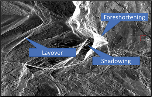
Only later has the field of landslide monitoring by this technology been explored (Iasio et al. 2012). Therefore, while for the first two applications (earthquake and subsidence) the role of topography (slope and aspect) played a marginal role, for landslides we realized the importance of these factors concurrently affecting the quality of the images. Difficulties, such as geometric distortions affecting kinematic interpretations, can occur in detecting the so-called Permanent Scatterers (PSs), ground points detected by the satellites (Colesanti and Wasowski 2006). This is the case of layover, foreshortening, and shadowing affected SAR images (Kropatsch and Strobl 1990), which could not allow the correct application of the interferometric technique.

To address this challenge, researchers have developed the R-Index, a measure of the likelihood of detecting PSs in mountainous regions (Notti et al. 2010, 2011). In order to predict the presence of PSs, the R-Index considers morphometric parameters, such as slope and aspect, and satellite parameters, such as the heading and incident angles, allowing the identification of slope sectors affected by layover or foreshortening. Layover occurs when signals belonging to different regions are mapped at the same point; foreshortening occurs when the radar beam reaches the base of a tall feature tilted toward the radar (e.g. a mountain) before it reaches the top. Because the radar measures distance in the slant-range, the slope will appear compressed, and the slope length will be represented incorrectly in the image plane. Finally, shadowing occurs when a portion of the study area is hidden from the satellite due to the presence of high relief (Figure 1).

Figure 1. SAR image effects by layover, foreshortening, and shadowing.

Previous studies focused on the evaluation of the applicability of interferometric techniques at the national scale: Cigna et al. (2014) (Great Britain), used ERS1/2 and ENVISAT images, while in Novellino et al. (2017), SENTINEL images were used to investigate the Mediterranean area. Recently Del Soldato et al. (2021), using SENTINEL images, carried out analysis on the alpine region.

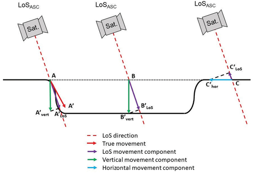
Furthermore, another critical aspect is the evaluation of ground displacements in areas characterized by complex topography along the Line of Sight (LOS), which represents the target sensor conjunction (Figure 2). In fact, interferometry can assess a component of the real displacement (Colesanti and Wasowski 2006). Even in the latter case, researchers have implemented algorithms to assess the true displacement perceptual that can occur in slope sectors characterized by complex morphologies (Plank et al. 2012).

Figure 2. True and LOS displacement components, modified from Duro et al. (2013).

To address these challenges, we produced an atlas for the entire Italian peninsula of the R-Index and the Percentage of measurability of movement. Such atlas represents a preliminary way to evaluate the quality and the applicability of satellite interferometry data collected by the CSK constellation.

This application finds its usefulness in the prominent use of CSK imagery in the latest research. Interferometric applications with CSK images mainly concentrate on monitoring structures (buildings, dams, etc.) and infrastructures (railways, highways, electricity lines, pipelines, etc.) subject to deformations induced by natural phenomena. In this field, the X-Band imaging potential is most visible owing to the very high density of identifiable reflectors. Such reflectors generate an extremely useful natural geodetic network for strategic structure monitoring. On the other hand, this type of atlas could also be a valuable tool in the decision-making phases of sites interested in artificial corner reflector network installation, enabling network design and corner reflector visibility optimization.

As a result, it is necessary to assess the interferometric technique’s applicability a-priori, and thus the identification of PS in contexts where the topography is complex.

2. COSMO-SkyMed constellation

The CSK program is funded by the Italian Space Agency (ASI). It uses SAR technology to manage, control, and explore the Earth’s resources. The project offers both civil and military use of the system. Although the acronym refers to the Mediterranean basin, it has been able to provide innovative services to several countries all over the world, such as Argentina (Ciappa, Pietranera, and Battazza 2010), Japan (Chini, Pulvirenti, and Pierdicca 2012), India (Dey et al. 2019), Ethiopia (Xu et al. 2020), China (Tapete et al. 2021) and others. Initially, the COSMO-SkyMed space mission consisted of a constellation of four identical satellites (CSK-1, CSK-2, CSK-3, and CSK-4) equipped with a medium-sized X-band SAR instrument. The X-band is a high-frequency microwave band with a wavelength of approximately 3.1 cm, which allows for high-resolution imaging. The constellation provides high-resolution SAR imagery with spatial resolutions ranging from 1 meter to 100 meters, depending on the imaging mode and the incidence angle (Pierdicca et al. 2013). Thanks to radar technology, such images can be acquired at any time of day or night, even in cloudy conditions.

The constellation is placed on the same orbital plane (offset by 90°) at an altitude of approximately 620 km and an inclination of 97.8°. Following the 4 First Generation of satellites, a Second Generation of COSMO-SkyMed satellites was added, consisting of 4 identical satellites equipped with X-band SAR instruments (CSG-1, CSG-2, CSG-3, and CSG-4). These second-generation satellites are also positioned on the same orbital plane. Observations of the area of interest are repeated several times each day. As every satellite is equipped with radar sensors, it is able to operate in all visibility conditions, at high resolution, and in real-time.

It is worth to point out, even if all first-generation satellites have completed their nominal operational life (which was planned to be equal to 5.25 years), three of the four satellites are still fully operational. Therefore, the actual constellation is formed by five satellites: three from the first generation and two from the second generation.

Finally, CSK derivable application services make a significant contribution to land protection, to risk mitigation against issues such as fires, landslides, droughts, floods, pollution, earthquakes, and subsidence, to natural resources management in both agricultural and forestry fields, and even to cadastral management.

3. MapItaly project

MapItaly project, developed by ASI (Agenzia Spaziale Italiana – Italian Space Agency) and the Italian Civil Protection Department, allows to access a 16-day interferometric mapping service that uses radar imagery produced by the COSMO-SkyMed constellation.

In particular, a historical series of images are acquired on Italian territory for interferometric analysis of unstable phenomena and endogenous risk (landslides, subsidence, seismic and volcanic phenomena, etc.). The objective is to update the national geographic reference archive regularly and intensively with specific interferometric historical data. Considering its strategic importance, this interferometric mission was given a high priority level, so it is now a “foreground mission.”

The project aims at providing reliable and up-to-date information on ground deformation, subsidence, and other geohazards (Virelli, Coletta, and Battagliere 2014). The MapItaly project covers the entire Italian territory and is divided into several areas of interest, including the Apennine Mountains, the Po River Valley, and the volcanic areas of central Italy. The MapItaly project currently uses the CSK-1, CSK-2, CSG-1 and CSG-2 satellites.

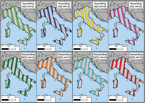
The four above-mentioned satellites cover the Italian Peninsula with a total of one hundred and two stripes, fifty in ascending and fifty-two in descending geometry (Figure 3). A − 10° heading angle characterizes the ascending tracks, while the descending ones are characterized by a 190° heading angle Milillo et al., 2016.

Figure 3. COSMO-SkyMed strips. The upper four are the ascending stripes, and the bottom four are the descending stripes. The abbreviations H4–01, H4–03, H4–04, and H4–05 are the original ones used by ASI.

The four satellites display four different incident angles, as shown in the following table (Table 1).

Table 1. Incident angle, expressed in degrees, for the different himage centre.

Himage Centre	Incident angle [°]
H4–01	26.65
H4–03	29.36
H4–04	32.23
H4–05	33.97

One of the key benefits of the MapItaly project is the ability to provide real-time information on ground deformation and other geohazards, such as during the earthquake that struck the city of L’Aquila in 2009 (Bovenga et al. 2010). This information supports decision-making processes such as disaster response, land use planning, and infrastructure management in critically dangerous areas. In fact, there have been many applications throughout Italy: for example, when monitoring subsidence in the Po River Valley (Boni et al. 2016), where extensive urban and industrial development has led to significant land deformation. Moreover, the project has also been used to monitor ground deformation in the Apennine Mountains, where landslides and other geohazards are common (Nutricato et al. 2013). In these areas, the project’s maps provide valuable information on the extent and severity of ground deformation, allowing authorities to take appropriate measures to mitigate the associated risks. The MapItaly project provides evidence of satellite remote sensing value in monitoring and managing geohazards. The project’s information is critical for decision-makers in disaster response, land use planning, and infrastructure management. It can potentially improve the resilience and safety of communities throughout the country. With ongoing improvements in satellite remote sensing technology and data processing algorithms, the MapItaly project will likely continue to provide valuable information for years to come with the new generation of satellites.

4. Methodology

In order to obtain the atlas of the R-Index and Percentage of Measurability of Movement maps, two different model builders were designed in ArcMap 10.5 environment, which allows a semi-automatic way to obtain the maps. The models have been exported as Python scripts and reported in the Annex B section. One strength of such models is its simplicity of application and the limited number of inputs. Specifically, the inputs consist of a) a Digital Terrain Model (hereafter DTM), which allows extraction of morphological data such as slope and aspect; b) SAR image acquisition data, such as heading angle (azimuth angle of satellite orbit); and incident angle (angle between radar signal and earth surface), both available in the metadata of the image itself. The algorithms used are briefly explained below; more details can be found in the original publications by Notti (Notti et al. 2010, 2011) and Plank (Plank et al. 2012).

As mentioned earlier, among the inputs needed to apply the algorithms is the DTM. The Italian peninsula DTM produced in 2005 by the Italian Ministry of the Environment (now Ministry of the Environment and Energetic Security), with a resolution of 20 m × 20 m, was used to perform the subsequent analysis. Such DTM has been used as it provides official data covering the entire peninsula and its use is free.

Furthermore, ASI provides the incident angles of each strip/track. The models’ computations and creation were performed using ArcMap 10.5 (ESRI Inc 2016) by means of the Model Builder function. A desktop PC with an Intel Core [email protected] GHz × 16 processor and 128 GB RAM 64bit has been used for processing. The runtime was mainly dependent on the size of the strip. The mean execution time was ~20 minutes for R-Index analysis and ~25 minutes for Percentage of Measurability of Movement analysis. This value can vary significantly depending on the PC specs and on the size of the area of interest.

4.1. R-Index

R-Index, the first of the two evaluated parameters, indicates the detection likelihood of Permanent Scatterers (PSs) in mountain areas (Notti et al. 2010, 2011). Although, as already stated, this algorithm was made for mountainous areas analysis, the process has been automatized and executed on the entire DTM, which also comprehends plain areas. It is obtainable by processing the slope and aspect values of the investigated area (geometric data of the surface), the heading angle of the satellite, and the incident angle (geometric data of the satellite). The formula used is the one proposed by (Notti et al. 2010, 2011):

(1) $R_{\mathit{Index}}=-\sin \left\{arctan\left[\tan \left(\mathit{S}\right)\times \sin \left(\mathit{A\alpha }\right)\right]-\mathit{\vartheta }\right\}$(1)

In this formula:

- S is the slope value in degrees;

- A is the slope aspect in degrees;

- Aα is the slope aspect corrected with the azimuth of the satellite orbit (heading angle);

- ϑ is the Line of Sight (LOS) angle of incidence.

R-Index values tend to vary between 1 and below 0. Lower than zero values indicate geometric issues related to foreshortening or layover. In these cases, the deformation of the obtained data is such that the values are unreliable. The cell deformation decreases as the R-Index value increases, and more PS can be detected. The numerical values of the R-Index can, as just stated, vary between 1 and below 0. The legend used in the Figures (modified from Notti et al. 2010) is divided into six classes:

• - R-Index ≤0: None to few PSs due to deformation effects that can affect the slope (layover and foreshortening);

• - 0.0 < R-Index ≤0.2: Strong Pixel Compression and few PSs detected;

• - 0.2 < R-Index ≤0.4: Low visibility;

• - 0.4 < R-Index ≤0.6: Medium visibility;

• - 0.6 < R-Index ≤0.8: Good visibility;

• - 0.8 < R-Index ≤1.0: Very good visibility.

4.2. Percentage of measurability of movement

The estimation of the percentage of measurability of movement is a valuable analysis for final performance enhancing of results as the DInSAR technique is unable to detect movements that occur along the satellite’s azimuth (which has almost a semi-polar orbit) (Crosetto et al. 2010). This percentage represents the quantity of detected total movement the satellite data can identify (Plank et al. 2012). Percentage of measurability of movement can be obtained using the following formulas (Plank et al. 2012), by first calculating the horizontal and the vertical components and multiplying them:

(2) $h_{\mathit{Ascending}}=\left|\cos \mathit{\beta }\right|\times 100\mathrm{\%}=\left|cos({90}^{\circ }-\mathit{\alpha }-\mathit{\epsilon })\right|\times 100\mathrm{\%}$(2)

(3) $h_{\mathit{Descending}}=\left|\cos \mathit{\beta }\right|\times 100\mathrm{\%}=\left|cos({90}^{\circ }-\mathit{\alpha }+\mathit{\epsilon })\right|\times 100\mathrm{\%}$(3)

In these formulas:

- h is the horizontal component of the percentage of measurability of movement;

- α is the slope aspect in degrees;

- ε is the angle between the LOS and the W-E.

Plank et al. (2012) observed that 100% of the movement is measurable when the slope dip direction equals the satellite line of sight direction. For the vertical component of the percentage, two other formulas are provided, depending on the geometry of the slope (oriented facing/averse the satellite). The two different formulas are still provided by Plank et al. (2012) and are shown below:

(4) $v_{\mathit{Averse}}=cos\left({\rho }_1\right)\times 100\mathrm{\%}=cos\left(\mathit{\psi }-\mathit{\delta }\right)\times 100\mathrm{\%}=cos\left({90}^{\circ }-\mathit{\vartheta }-\mathit{\delta }\right)\times 100\mathrm{\%}$(4)

(5) $v_{\mathit{Towards}}=cos\left({\rho }_2\right)\times 100\mathrm{\%}=cos\left(\mathit{\psi }+\mathit{\delta }\right)\times 100\mathrm{\%}=cos\left({90}^{\circ }-\mathit{\vartheta }+\mathit{\delta }\right)\times 100\mathrm{\%}$(5)

Where:

- ϑ is the LOS incidence angle;

- δ is the dip angle of the slope;

- ψ is the difference 90°- ϑ;

- ρ is different whenever the slope is facing or not the satellite and represents the interaction between ψ and δ.

The final percentage of measurability movement is calculated by multiplying the horizontal and vertical components obtained with the shown formulas.

(6) $\mathit{Percentage}=\mathit{h}\times \mathit{v}$(6)

The numerical values of the Percentage of Measurability of Movement can vary between 0% and 100%. The legend used in the Figures identifies 5 classes:

• - 0%<Percentage ≤20%: Low to no movement can be detected;

• - 20%< Percentage ≤ 40%;

• - 40%< Percentage ≤ 60%;

• - 60%< Percentage ≤ 80%;

• - 80%< Percentage ≤ 100%: Up to 100% of the movement can be detected.

4.3. Maximum likelihood-based average visibility score calculation

Integrating the Maximum Likelihood-based Average Visibility Score Calculation with the InSAR methodology is pivotal in ensuring the robustness and accuracy of our environmental analysis. This visibility scoring process represents a foundational step in assessing and enhancing the quality of satellite imagery prior to R-Index and Percentage of Measurability mapping. This approach is particularly vital in InSAR applications, where the quality of input data directly affects the reliability of deformation measurements and environmental assessments. This study describes a methodology based on maximum likelihood estimation to calculate each track’s weighted average visibility score. Calculating the average visibility score for each track is based on a maximum likelihood approach using a Gaussian Mixture Model (GMM) classifier with a single component. The spectral values for each class were defined based on the RGB values of the colors representing the different levels of visibility, ranging from clear (white) to very poor (red). These spectral values were used to train a GMM classifier with a single component using the Scikit-learn library. The pixel values for each track were loaded and reshaped to form a single input vector for the classifier. The trained classifier was then used to predict the class labels for each pixel in the track, which were reshaped to form a 2D array of size (n_samples, n_features), where n_samples is the number of tracks and n_features is the number of pixels per track. The visibility scores for each class were defined as follows: very poor (−1.0), poor (−0.5), fair (0.1), good (0.3), very good (0.8), and transparent (1.0). The proportion of pixels for each section was calculated by dividing the number of pixels in each section by the total number of pixels in that section for all tracks. The proportion of pixels for each class for each track was then calculated by summing the proportions of pixels for each section that belongs to that class. By employing a GMM classifier, we effectively categorize pixel data based on visibility, ensuring that our InSAR analysis is fed with the most reliable and explicit imagery. This classification and the subsequent visibility scoring, ranging from “very poor” to “transparent,” allow for a nuanced and quantitative evaluation of satellite image quality. The weighted proportion of pixels for each track was then calculated by multiplying the proportion of pixels for each class for that track by its corresponding visibility score and summing these values over all classes. This weighted proportion was then normalized by dividing it by the sum of all weighted proportions across all tracks. The weighted average visibility score for each track was calculated by taking the dot product of the normalized weighted proportions and the visibility scores for each class. This was repeated for each track to obtain the weighted average visibility score. The formula for calculating the weighted average visibility score for a track is:

(7) $\mathit{WAV}{S}_i=\frac{\sum _{\mathit{j}=1}^6{P}_{\mathit{i},\mathit{j}}\ast \mathit{V}{S}_j}{\sum _{\mathit{j}=1}^6\sum _{\mathit{k}=1}^n{P}_{\mathit{k},\mathit{j}}\ast \mathit{V}{S}_j}$(7)

Where $\mathit{WAVS}\mathrm{\_i}$is the weighted average visibility score for track i, $\mathit{P}\mathrm{\_}\left\{\mathit{i},\mathit{j}\right\}$is the proportion of pixels for class j in track i, $\mathit{VS}\mathrm{\_}\mathit{j}$is the visibility score for class j, n is the total number of tracks, and k is the index over all tracks. Finally, the results were summarized in graph-based figures containing the track number and corresponding weighted average visibility score.

In summary, this visibility scoring is not just a measure of image clarity but also an indirect indicator of potential interferometric coherence issues. Higher visibility scores correlate with an increased likelihood of obtaining coherent and interpretable InSAR results. Thus, this methodology acts as a crucial filter, enabling us to prioritize high-quality tracks for our detailed InSAR analysis and ensuring that our R-Index and Percentage of Measurability mappings are based on the most reliable data.

5. Results and discussion

The products of these algorithms are the R-Index (Figure 4, legend from Notti et al. 2010, modified) and the Percentage of measurability of movement (Figure 5) for the entire Italian Peninsula, divided by the satellite acquisition tracks. Full-page maps are attached to Annex A (Figure A-I, Figure A-II, Figure A-III, and Figure A-IV). One hundred raster files describe the R-Index and the Percentage of measurability of movement for the Ascending orbits, while one hundred and six raster files describe the Descending orbits.

Figure 4. R-Index maps (full page maps in annex A): ascending (left), descending (right).

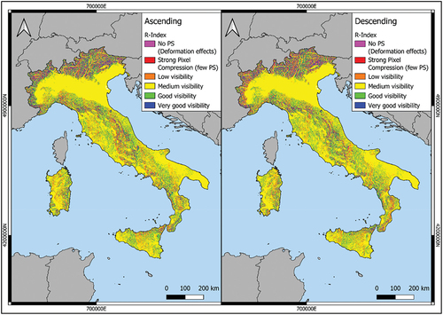
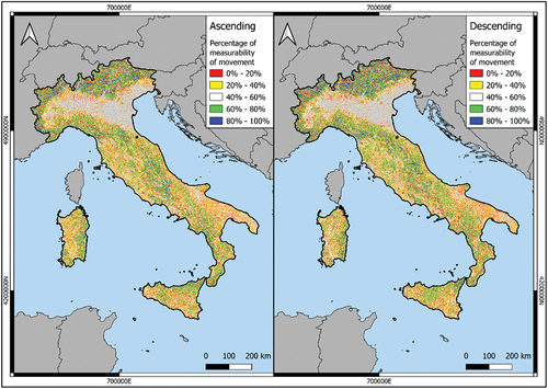
Figure 5. Percentage of measurability of movement maps (full page maps in annex a): ascending (left), descending (right).

The higher quality classes of the R-Index follow the LOS of the satellite. In the case of the Ascending Figure 6(b,c) and the Descending Figure 6(d,e) geometries, the quality of the visibility of the slopes is almost the opposite of each other, rendering a solid coverage of the entire examined area. In order to highlight the results, two sites of UNESCO interest characterized by high geological hazards (Ciervo et al. 2017; Di Napoli et al. 2021) were shown in Figure 6. The most widespread class is the third one (Medium visibility), followed by the fourth (Good visibility) and the second one (Low visibility – few PS). The remaining classes are shown in the following table (Table 2).

Figure 6. R-index sketch maps: a) Italy map; b and c) Ascending; d and e) descending.

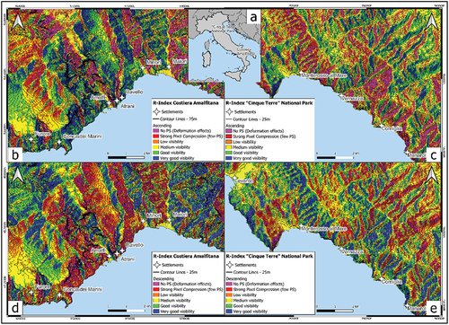
Table 2. Spatial extent of different classes of R-indexes.

	Geometric deformation (no PS)	Strong pixel compression (few PS)	Low visibility (few PS)	Medium visibility	Good visibility	Very good visibility
R-Index (Ascending)	2.06%	4.16%	11.10%	64.25%	13.64%	4.78%
R-Index (Descending)	2.30%	4.30%	12.34%	62.81%	13.46%	4.78%

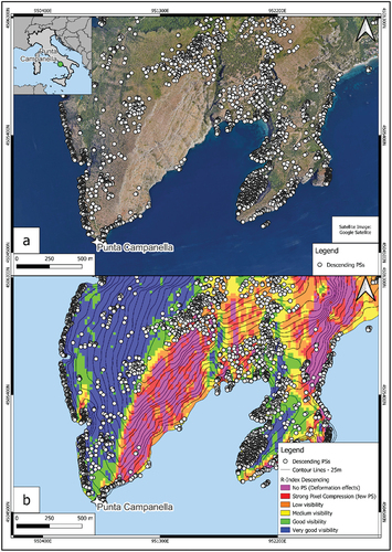
Figure 7 shows a comparison between the R-Index Figure 7(b) result and an optical image Figure 7(a) in order to assess the accuracy of the obtained results.

Figure 7. a) descending PSs detected in the area of Punta Campanella (https://gn.mase.gov.it/), Campania Region, and b) R-Index map for the descending geometry of the same area.

For the Percentage of measurability of movement, the highest quality of the data is found along the slopes with a dip direction close to E-W, as expected Figure 8(b–e).

Figure 8. Percentage of measurability of movement sketch maps: a) Italy map; b and c) Ascending; d and e) descending.

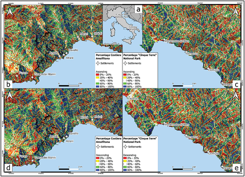
Both in Ascending and Descending, the most widespread class is the third one (30.88% and 30.52%, respectively). The fifth class is the least widespread (6.13% in Ascending and 6.15% in Descending). This is expected to be the highest quality class (the fifth − 80%-100% of the percentage of measurability of movement) that requires both the movement’s vertical and horizontal components to be perfectly aligned with the satellite. All the data related to the spatial distribution of the classes is shown in Table 3. Ascending and Descending data for the R-Index (Table A-I and Table A-II, respectively) and the Percentage of measurability of movement (Table A-III and Table A-IV) for all the tracks are shown in Annex A.

Table 3. Spatial extent of different classes of percentage of measurability of movement.

	0% − 20%	20% − 40%	40% − 60%	60% − 80%	80% − 100%
Percentage of measurability of movement (Ascending)	22.55%	22.83%	30.88%	17.61%	6.13%
Percentage of measurability of movement (Descending)	23.01%	22.74%	30.52%	17.59%	6.15%

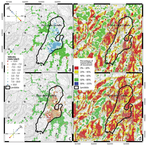
In order to validate the results for Percentage of measurability of movement maps, Figure 9 shows on one hand the mean displacement rates Figure 9 (a–c) and Percentage of measurability of movement Figure 9 (b–d) maps for the two acquisition geometries, ascending and descending, respectively. As can be seen, the area is affected by significant mass movements, detected by official land management agencies, as also reported in the literature (Mele, Miano, et al. 2022). The Percentage of measurability of movement are higher in ascending geometry than what is found in descending geometry, this is due to a better dip aspect of the slopes that dip in the NE-SW direction. At the same time, the mean displacement rates recorded in ascending geometry would seem to be higher than in descending geometry, confirming that it turns out to be better visibility in ascending geometry.

Figure 9. Mean displacement rate and percentage of measurability of movement maps in ascending (a and b) and descending (c and d) orbits. Interferometric data have been obtained from (https://gn.mase.gov.it/) and landslide boundary from (Fusco et al. 2023).

5.2. Evaluation of results based on the average visibility score

Figures A-V to A-XII (Annex A) show the results of the weighted average visibility scores for each track in each group, which allow us to compare visibility scores within and between these groups.

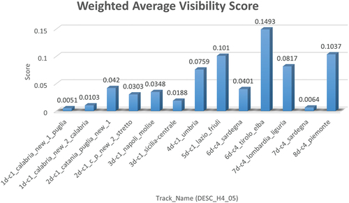
The scores range from 0 to 0.1904, with higher scores indicating better visibility. Looking at Figure A-V, track 5a-c2_napoli_austria shows the highest weighted average visibility score of 0.1725, while 4a-c4_sicilia had the lowest score of 0.022. In Figure A-VI, track 5a_c1_gaeta_austria had the highest score of 0.1904, while track 8a-c2_salento had the lowest score of 0.006. Figure A-VII shows that track 4a-c1_roma_austria had the highest weighted average visibility score of 0.1608, while track 9a-c3_salento had the lowest score of 0.0007. Figure A-VIII illustrates that track 4a-c4_roma_tirolo had the highest weighted average visibility score of 0.1482, while track 7a-c4_puglia had the lowest score of 0.0061. In Figure A-IX, track 6d_c2_a_bologna_austria had the highest weighted average visibility score of 0.1281, while track 5d-c3_trieste had the lowest score of 0.0033. Figure A-X indicates that track 6d-c2_a_bologna_austria had the highest weighted average visibility score of 0.1416, while track 4d-c3_sicilia_occ had the lowest score of 0.0093. In Figure A-XI, track 6d-c3_toscana_trentino had the highest weighted average visibility score of 0.1416, while track 4d-c2_sicilia_ovest had the lowest score of 0.0383. Figure A-XII shows that track 6d-c4_tirolo_elba had the highest weighted average visibility score of 0.1493, while track 1d-c1_calabria_new_1_puglia had the lowest score of 0.0051. Overall, the results show that visibility scores vary widely between tracks. Some tracks have very good visibility, with scores close to 1.0, while others have very poor visibility, with scores close to 0. We can also see that some tracks have scores close to 0, indicating fair or poor visibility, while others have scores closer to 1.0, indicating good to very good visibility.

As depicted in Figures A-V to A-XII, the integration of the Maximum Likelihood-based Average Visibility Score Calculation with our InSAR analysis framework is evident. The variation in visibility scores across different tracks not only provides direct assessment of data quality but also indirectly informs the accuracy and reliability of our InSAR-derived R-Index and Percentage of Measurability mappings. For instance, tracks like 5a-c2_napoli_austria with higher visibility scores yielded more reliable and interpretable InSAR results than tracks with lower scores.

This comprehensive approach, merging visibility assessment with InSAR analysis, is particularly advantageous in regions where environmental factors can severely affect satellite image quality. By correlating visibility scores with InSAR results, more accurate conclusions about environmental changes and ground deformation patterns can be drawn, thereby enhancing the overall reliability of our environmental monitoring efforts.

6. Conclusion

In this study, we produced an atlas for the entire Italian Peninsula using two parameters, the R-Index, and the Percentage of measurability of movement, to evaluate the quality of satellite interferometry data collected by the CSK constellation. The COSMO-SkyMed constellation is a powerful tool for Earth observation, with its X-band SAR capabilities, high-resolution imaging modes, and short revisit time. Its diverse applications include scientific research, environmental monitoring, disaster response, and security and defense operations. The limitations of the constellation, such as its high cost and dependence on radar imaging, must be considered. However, the benefits of the COSMO-SkyMed constellation make it an essential tool for Earth observation and remote sensing, and its contributions to the field are likely to continue in the future.

The R-Index describes the likelihood of detecting Permanent Scatterers, while the Percentage of measurability of movement indicates the percentage of actual motion that interferometry can detect at a certain point in the analyzed region. In order to make the atlas, a high-resolution DTM was used, which enabled the identification of areas that could be monitored with the interferometric technique.

The results of our analysis showed that the R-Index and the Percentage of measurability of movement could be used to evaluate the applicability of satellite interferometry data collected by the CSK constellation. The atlas provides preliminary information that can be followed by a detailed study.

In summary, our study confirms that the CSK constellation is a powerful tool for Earth’s surface observation and monitoring environmental changes, particularly in mountainous areas. Using the R-Index and the Percentage of measurability of movement provides valuable information on the applicability of satellite interferometry data collected by the constellation, which can help identify critical areas for satellite interferometry monitoring and studying. This research has important implications for disaster response, environmental monitoring, and scientific research.

In particular, the R-Index highlights critical areas where distortion phenomena can make data processing complex (foreshortening, layover) or affect the theoretical amount of PSs obtained. This analysis is based on the morphological characteristics of the landscape (mainly slope and aspect) at high resolution (20 meters), so other parameters such as land use have not been considered as the resolution of the European Corine Land Cover is lower (100 meters) than the one used in this study. Specific localized studies would allow a characterization of the land cover with a compatible resolution.

The percentage of detectable movement allows identification of the quantity (in percentage) of actual movement that can be recognized using satellite interferometry.

The results show that a high percentage of the Italian peninsula falls within the higher R-Index classes (good data quality), while the Percentage of measurability of movement shows a more widespread distribution between the different classes, mostly due to the impossibility of measuring movements along the N-S direction. Mapping the Italian peninsula’s R-Index and Percentage of Measurability of Movement yielded a panorama of natural and human hazard assessment and remote sensing possibilities.

Strength points of the approaches described in this study are listed below.

• - Simplicity and Accessibility: one of its significant attributes is that it does not necessitate a myriad of varied input data in a world dominated by complexities. It signifies a notable leap toward ensuring more individuals and institutions can leverage such profound analyses without being bogged down by convoluted processes.

• - Grounding in Established Methods: this investigation took cues from previous researchers, adopted established algorithms, and synergized them. This amalgamation has not only strengthened the study’s foundation but also instilled confidence in the derived results.

• - In-depth Terrain Analysis: delving into the R-Index and Percentage of Measurability of Movement has peeled back layers on the terrain behavior, especially in regions marked by elevation variances. The intricate relationship between the quality of visibility and the Line of Sight (LOS) of the satellite has brought to the forefront nuances that were earlier perhaps overlooked. This relationship is pivotal, considering it dictates the satellite’s prowess in pinpointing deformations across different terrains.

• - Geometry Insight: a salient feature of the study, captured eloquently in Figures 4-8, is the distinction and coverage provided by both Ascending and Descending orbits. The complementary nature of these orbits ensures a comprehensive blanket coverage of the entire studied expanse, ensuring no terrain nuance slips through the analytical net. Their contrasting qualities concerning slope classifications highlight the importance of multiple vantage points in satellite data collection.

• - Data Quality – the Crucial Metric: Further examination of the weighted average visibility scores across different tracks, as illustrated in our results, reveals a broader implication for InSAR applications. Tracks with varied visibility scores demonstrate how environmental factors, such as atmospheric conditions or surface cover variations, can significantly impact the quality of satellite imagery and, consequently, the reliability of InSAR mappings. For instance, lower visibility scores indicated potential challenges in achieving coherent InSAR results in areas with frequent cloud cover or dense vegetation. Conversely, tracks with higher visibility scores, reflective of more apparent imaging conditions, correspond to more reliable InSAR data. This direct correlation underscores the importance of incorporating visibility scoring in InSAR studies, particularly in environmental monitoring and land deformation analyses. By integrating this visibility assessment, we enhance our ability to interpret InSAR data accurately, making informed decisions about which areas require closer examination or may yield more reliable results. Ultimately, this approach paves the way for more nuanced and accurate environmental assessments, leveraging the full potential of InSAR technology by ensuring the quality of input data.

In the grand narrative of engineering geology research, this study threads a significant contribution, offering both appropriate methodologies and tools for adoption and implementation. Its resilience and malleability to diverse terrains and data sets suggest its viability as a reference point in similar academic pursuits.

As we look ahead, the frontier seems ripe for exploration. It prompts us to ponder how these methodologies fare when transplanted to geographies with a different terrain palette. Moreover, with the relentless march of technology and advancements in satellite imaging, one can only anticipate that the future beckons a new era of refined, detailed, and nuanced analyses.

Acknowledgments

The project was carried out using COSMO-SkyMed Products, © of the Italian Space Agency (ASI), delivered under a license to use by ASI.

Disclosure statement

No potential conflict of interest was reported by the author(s).

Data availability statement

Data repository structure: The atlas geodatabase will be available in a repository. It is intended to make it open and available to all researchers and professional users. Data generated in this work will be accessible from the repository in which a single packaged zip archive will be uploaded. It will contain a “READ_ME” text file that will provide guidance information for users and two subfolders: “R-Index” and “Percentage.”

All features are projected in the WGS 84/UTM zone 33 N coordinate system.

The majority of the work was carried out by ArcMap 10.5, but all items were produced in a format importable into any other GIS software.

Additional information

Funding

This study was carried out within the RETURN Extended Partnership and received funding from the European Union Next-GenerationEU (National Recovery and Resilience Plan – NRRP, Mission 4, Component 2, Investment 1.3 – D.D. 1243 2/8/2022, PE0000005). The work was partly funded by the University Research Funding Program—Line A of the University of Naples Federico II.Moreover, the work was partly funded by the University Research Funding Program - Line A of the University of Naples Federico II, “INTEGRATED PROCEDURE FOR MONITORINGOF LINEAR INFRASTRUCTURES SAFETY (I-PRO MONALISA)‘- Scientific Responsible Dr Diego Di Martire and by the Ph.D. scholarship ’P.O.N. Dottorati innovativi a caratterizzazione industriale 2014–2020”, Scientific Responsible Dr Diego Di Martire.

Annex A

The following tables are cited in the Results and Discussion chapter and contain data regarding the single strips. Every family of strips has the same incident angle.

Table A1. Ascending R-Index data for the single strips.

R-Index (Ascending)		Geometric deformation (no PS)	Strong pixel compression (few PS)	Low slope (few PS)	Medium slope	Good slope	Very good slope	tot [pixel]
ASC_H4_01	2°-c1_monaco_valdaosta	6.92%	7.62%	11.78%	51.01%	14.76%	7.90%	25666787
	2°-c1_sardegna2	0.67%	3.16%	15.33%	74.50%	5.61%	0.73%	24175671
	3°-c3_liguria_piemonte	3.63%	5.74%	11.11%	67.00%	8.68%	3.83%	23655673
	4°-c2_argentario_svizzera	3.76%	5.89%	15.89%	60.41%	10.19%	3.86%	49409471
	4°-c4_sicilia	0.05%	0.12%	1.40%	98.02%	0.31%	0.10%	3326633
	5°-c2_napoli_austria	3.44%	6.36%	15.00%	61.74%	10.08%	3.38%	68763175
	5°-c2_sicilia_centrale	0.65%	3.10%	23.78%	64.11%	7.76%	0.60%	12595381
	6°-c1_centro	1.81%	4.89%	19.68%	61.48%	10.36%	1.78%	26786244
	6°-c1_friuli	5.17%	5.18%	8.26%	68.20%	7.96%	5.23%	12976229
	6°-c1_sicilia_ne	3.04%	5.86%	9.13%	68.91%	9.43%	3.64%	6935961
	7a-c1_calabria_gargano	1.30%	4.72%	17.54%	64.68%	10.30%	1.47%	38195937
	8a-c1_salento	0.00%	0.01%	0.63%	99.33%	0.03%	0.00%	9485775
ASC_H4_03	2a-c2_liguria_svizzera	3.33%	5.50%	12.44%	58.08%	14.13%	6.51%	24757581
	2a-c2_sardegna	0.89%	4.87%	16.91%	61.18%	13.71%	2.44%	23667594
	3a-c1_elba_svizzera	2.26%	4.68%	11.39%	66.33%	11.22%	4.12%	27065423
	4a-c3_lazio_trentino	3.27%	4.90%	13.59%	60.01%	13.19%	5.04%	54739572
	4a-c3_sicilia	0.24%	0.83%	7.28%	86.55%	4.50%	0.60%	7437002
	5a_c1_gaeta_austria	3.79%	6.79%	14.05%	54.77%	14.27%	6.34%	59698459
	5a-c4_sicilia	0.40%	2.34%	15.65%	67.83%	12.71%	1.07%	15268339
	6a-c2_friuli_venezia_giulia	3.72%	4.79%	9.76%	65.91%	9.82%	5.99%	9468567
	6a-c2_messina_molise_new_1	0.97%	3.06%	18.58%	61.16%	14.44%	1.79%	25401161
	6a-c2_messina_molise_new_2_stretto	2.71%	5.61%	12.22%	65.25%	10.33%	3.88%	5070803
	7a-c2_calabria-gargano	0.40%	1.55%	6.96%	81.75%	8.21%	1.12%	25408716
	8a-c2_salento	0.00%	0.00%	0.19%	99.38%	0.40%	0.03%	9253032
ASC_H4_04	1a-c1_sardegna	0.25%	1.07%	3.11%	90.68%	4.05%	0.83%	4180920
	1a-c1_valdaosta	4.48%	9.51%	14.71%	37.25%	18.97%	15.08%	11365599
	2a-c3_liguria_piemonte	2.13%	3.93%	8.52%	62.16%	15.17%	8.09%	23439416
	2a-c3_sardegna	0.67%	3.20%	9.80%	62.62%	18.59%	5.13%	20430940
	3a-c2_elba_svizzera	2.68%	4.43%	8.58%	63.90%	13.70%	6.71%	36819318
	4a-c1_roma_austria	1.92%	4.13%	9.78%	62.26%	15.57%	6.34%	62149065
	4a-c1_sicilia	0.41%	1.53%	9.16%	71.76%	15.43%	1.72%	10278911
	5a-c3_campania_marche	1.11%	4.27%	11.44%	58.04%	19.36%	5.78%	35065063
	5a-c3_friuli	4.83%	5.59%	7.65%	59.69%	11.11%	11.13%	17940949
	5a-c3_sicilia	0.26%	1.47%	9.03%	72.38%	15.37%	1.50%	18788678
	6a-c3_calabria_molise_new_1	0.60%	2.52%	10.16%	66.34%	17.56%	2.83%	25022187
	6a-c3_calabria_molise_new_2	1.27%	3.49%	8.84%	66.10%	15.33%	4.97%	9034866
	7a-c3_puglia	0.01%	0.03%	0.27%	98.09%	1.57%	0.04%	9496490
	9a-c3_salento	0.00%	0.00%	0.06%	98.83%	1.00%	0.11%	1149109
ASC_H4_05	1a-c2_piemonte	3.92%	7.93%	11.74%	36.17%	23.22%	17.02%	21828384
	1a-c2_sardegna	0.19%	1.49%	5.28%	80.22%	10.73%	2.09%	18626344
	2a-c4_liguria_piemonte	2.06%	3.82%	6.42%	66.21%	13.43%	8.07%	24798316
	2a-c4_sardegna	0.33%	1.72%	6.10%	71.77%	15.84%	4.24%	7187775
	3a-c4_toscana_lombardia	1.84%	3.82%	8.03%	63.46%	15.82%	7.04%	44381045
	4a-c2_sicilia_palermo	0.38%	1.44%	8.21%	62.36%	24.87%	2.74%	12442967
	4a-c4_roma_tirolo	1.22%	3.15%	8.14%	64.03%	17.32%	6.13%	66537316
	5a-c1_sicilia	0.30%	1.37%	5.40%	71.90%	18.23%	2.81%	18312456
	5a-c4_campania_marche	0.62%	2.72%	8.50%	61.57%	21.79%	4.80%	34517008
	5a-c4_friuli	2.77%	3.95%	5.53%	68.92%	10.03%	8.79%	13403351
	6a-c4_calabria_puglia	0.57%	2.70%	9.23%	62.03%	21.16%	4.30%	43387217
	7a-c4_puglia	0.00%	0.02%	0.21%	95.14%	4.55%	0.08%	9202759

Figure A1. R-Index map of the Italian Peninsula, ascending geometry.

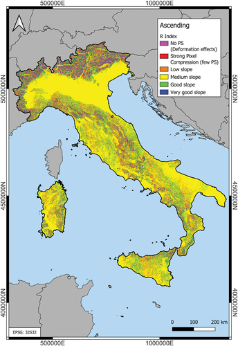
Table A2. Descending R-Index data for the single strips.

R-Index (Descending)		Geometric deformation (no PS)	Strong pixel compression (few PS)	Low slope (few PS)	Medium slope	Good slope	Very good slope	tot [pixel]
DESC_H4_01	1d-c4_salento	0.03%	0.19%	1.70%	98.04%	0.03%	0.00%	5729574
	2d-c4_puglia_calabria	1.80%	4.68%	16.00%	68.97%	7.06%	1.49%	25249299
	3d-c2_foggia	1.20%	3.70%	17.20%	68.25%	8.42%	1.23%	23815128
	3d-c2_sicilia_eolie	0.90%	3.43%	17.03%	69.68%	8.08%	0.88%	19513305
	4d-c1_sicilia_palermo	1.02%	3.27%	19.65%	67.17%	7.84%	1.05%	10205673
	4d-c4_abruzzo_campania	1.77%	5.12%	19.66%	63.10%	8.92%	1.42%	19385106
	5d-c3_trieste	1.02%	1.22%	8.82%	84.34%	4.13%	0.47%	2872509
	5d-c3_umbria	3.26%	6.64%	18.60%	55.09%	13.11%	3.30%	27835979
	6d-c1_roma_austria	3.27%	4.55%	12.96%	67.98%	8.24%	3.00%	52360531
	7d-c2_elba_austria	6.77%	7.34%	12.86%	55.85%	11.29%	5.89%	40812547
	7d-c2_sardegna	1.85%	6.23%	18.04%	61.25%	11.09%	1.54%	26770971
	8d-c1_liguria_svizzera	5.07%	6.21%	11.24%	62.53%	9.95%	5.01%	25381154
	9d-c2_monaco_svizzera	8.03%	8.53%	15.73%	50.77%	10.67%	6.27%	24471852
DESC_H4_03	1d-c3_puglia	0.00%	0.07%	82.62%	0.05%	0.00%	17.26%	8881489
	2d-c3_puglia_calabria	1.19%	3.64%	12.92%	67.50%	12.23%	2.52%	37549066
	3d-c3_campania_molise	0.79%	2.31%	12.06%	71.99%	11.23%	1.61%	20983616
	3d-c3_sicilia_centrale	0.41%	2.34%	15.81%	65.98%	14.44%	1.02%	14168915
	4d-c3_lazio	2.33%	6.02%	16.21%	55.25%	15.90%	4.29%	18628185
	4d-c3_sicilia_occ	0.45%	1.16%	8.27%	82.00%	7.34%	0.77%	7945990
	5d-c4_friuli	3.45%	4.26%	7.16%	71.64%	8.57%	4.93%	10687826
	5d-c4_marche_roma	1.34%	3.82%	13.69%	64.94%	13.66%	2.55%	27645852
	6d-c2_argent_bologna_austria	3.25%	4.73%	11.55%	63.91%	11.95%	4.62%	55030694
	7d-c3_liguria_lombardia	5.20%	7.78%	12.96%	51.22%	14.34%	8.51%	34287096
	7d-c3_sardegna	0.54%	2.74%	10.92%	73.21%	11.37%	1.22%	29324915
	8d-c3_liguria_piemonte	1.66%	3.53%	7.81%	76.23%	8.16%	2.61%	24850567
	9d-c1_valdaosta	10.47%	11.61%	16.89%	29.91%	19.08%	12.04%	18472378
	1d-c2_taranto_est	0.00%	0.09%	73.72%	0.36%	0.01%	25.82%	8616461
	2d-c2_sicilia_puglia	0.76%	2.83%	8.78%	69.07%	15.01%	3.56%	33260761
DESC_H4_04	2d-c2_siclia_puglia_solo_sicilia	0.98%	2.82%	5.01%	78.75%	8.72%	3.72%	9282963
	3d-c4_sicilia	0.24%	1.44%	11.00%	63.16%	22.46%	1.70%	11606662
	3d-c4_molise_campania	0.64%	2.10%	10.25%	64.66%	19.55%	2.80%	17847155
	4d-c2_centro	1.20%	4.58%	12.42%	57.95%	18.79%	5.06%	25729248
	4d-c2_sicilia_ovest	0.07%	0.24%	0.91%	93.84%	4.48%	0.46%	4924795
	5d-c2_roma_n_austria_new_1_north	2.85%	3.82%	5.27%	74.49%	7.34%	6.24%	14499141
	5d-c2_roma_n_austria_new_2_south	0.37%	2.56%	10.82%	64.92%	18.94%	2.40%	26566239
	6d-c3_toscana_trentino	2.26%	4.76%	10.52%	59.02%	16.55%	6.89%	51011786
	7d-c1_liguria-svizzera	3.25%	5.65%	10.44%	55.94%	16.22%	8.51%	29039275
	7d-c1_sardegna	0.10%	0.86%	4.48%	82.07%	11.16%	1.33%	16406776
	8d-c2_liguria-svizzera	2.97%	6.03%	11.08%	57.60%	15.00%	7.32%	30522978
	9d-c3_francia_valdaosta	5.76%	7.16%	11.55%	32.85%	29.73%	12.96%	5711885
DESC_H4_05	1d-c1_calabria_new_1_puglia	0.00%	0.05%	0.39%	95.56%	3.95%	0.04%	7130536
	1d-c1_calabria_new_2_calabria	0.26%	1.33%	6.62%	77.17%	12.73%	1.90%	7008574
	2d-c1_catania_puglia_new_1	0.32%	1.89%	7.35%	66.94%	20.14%	3.37%	23319771
	2d-c1_catania_puglia_new_2_stretto	0.63%	2.43%	6.05%	74.35%	12.95%	3.59%	17062655
	3d-c1_napoli_molise	0.38%	1.58%	8.06%	65.71%	21.30%	2.98%	19218517
	3d-c1_sicilia-centrale	0.23%	1.11%	8.40%	59.44%	28.58%	2.25%	10414778
	4d-c1_umbria	1.09%	4.14%	10.32%	54.41%	23.04%	7.01%	28481787
	5d-c1_lazio_friuli	1.22%	2.41%	6.36%	71.37%	14.35%	4.28%	50094502
	6d-c4_sardegna	0.87%	4.49%	10.69%	62.61%	15.50%	5.84%	16320421
	6d-c4_tirolo_elba	2.48%	4.71%	9.14%	57.62%	17.30%	8.75%	48776138
	7d-c4_lombardia_liguria	2.51%	4.92%	8.60%	56.45%	17.70%	9.82%	25999116
	7d-c4_sardegna	0.02%	0.26%	2.36%	86.29%	9.82%	1.26%	6406656
	8d-c4_piemonte	3.36%	5.68%	9.33%	58.11%	14.15%	9.36%	30521208

Figure A2. R-Index map of the Italian Peninsula, descending geometry.

Table A3. Ascending percent of measurability of movement data for the single strips.

Percentage of measurability of movement (Ascending)		0% − 20%	20% − 40%	40% − 60%	60% − 80%	80% − 100%	tot [pixel]
ASC_H4_01	2a-c1_monaco_valdaosta	24.20%	24.63%	23.71%	17.97%	9.49%	21343265
	2a-c1_sardegna2	24.16%	32.51%	34.10%	8.27%	0.96%	18260402
	3a-c3_liguria_piemonte	24.53%	27.72%	26.73%	15.27%	5.74%	15340877
	4a-c2_argentario_svizzera	24.00%	26.79%	29.09%	14.94%	5.18%	37023584
	4a-c4_sicilia	19.95%	43.79%	34.06%	1.70%	0.51%	732352
	5a-c2_napoli_austria	23.25%	25.82%	29.68%	16.39%	4.86%	47927447
	5a-c2_sicilia_centrale	26.69%	27.60%	35.41%	9.58%	0.71%	10467024
	6a-c1_centro	24.71%	27.31%	33.13%	12.62%	2.23%	22027132
	6a-c1_friuli	25.13%	27.82%	23.97%	14.67%	8.40%	7647479
	6a-c1_sicilia_ne	21.37%	21.40%	28.56%	21.71%	6.96%	3422953
	7a-c1_calabria_gargano	25.36%	28.72%	31.79%	12.45%	1.68%	31802614
	8a-c1_salento	22.93%	48.82%	28.15%	0.09%	0.00%	4191780
ASC_H4_03	2a-c2_liguria_svizzera	22.86%	21.81%	30.30%	17.48%	7.55%	20501227
	2a-c2_sardegna	23.00%	23.18%	34.02%	16.99%	2.81%	20453480
	3a-c1_elba_svizzera	23.76%	21.81%	29.78%	18.27%	6.38%	17702952
	4a-c3_lazio_trentino	21.99%	21.50%	32.38%	17.82%	6.30%	42609935
	4a-c3_sicilia	23.93%	26.24%	42.25%	6.74%	0.85%	5077655
	5a_c1_gaeta_austria	21.59%	20.10%	29.57%	20.77%	7.98%	46137350
	5a-c4_sicilia	24.71%	24.11%	36.06%	13.95%	1.16%	13245512
	6a-c2_friuli_venezia_giulia	24.66%	21.38%	28.97%	16.29%	8.70%	5871318
	6a-c2_messina_molise_new_1	22.58%	22.88%	35.71%	16.77%	2.05%	22184149
	6a-c2_messina_molise_new_2_stretto	22.37%	20.88%	29.89%	19.96%	6.89%	2994885
	7a-c2_calabria-gargano	23.80%	25.46%	39.35%	10.06%	1.34%	18156326
	8a-c2_salento	19.44%	25.92%	53.89%	0.71%	0.04%	4078385
ASC_H4_04	1a-c1_sardegna	19.91%	21.34%	38.48%	16.74%	3.54%	1212941
	1a-c1_valdaosta	21.04%	17.02%	24.18%	23.22%	14.54%	11189198
	2a-c3_liguria_piemonte	23.24%	21.20%	28.97%	17.59%	8.99%	18068968
	2a-c3_sardegna	21.98%	21.32%	30.49%	20.76%	5.45%	15586148
	3a-c2_elba_svizzera	23.01%	20.88%	27.17%	18.59%	10.35%	24732782
	4a-c1_roma_austria	20.43%	20.08%	31.16%	20.50%	7.82%	46526865
	4a-c1_sicilia	23.55%	22.59%	34.06%	17.83%	1.98%	8095796
	5a-c3_campania_marche	21.68%	20.68%	30.21%	20.98%	6.46%	29425349
	5a-c3_friuli	21.60%	18.40%	24.13%	19.40%	16.46%	10920640
	5a-c3_sicilia	23.02%	22.46%	35.40%	17.30%	1.83%	15311143
	6a-c3_calabria_molise_new_1	21.49%	21.69%	34.75%	18.74%	3.34%	21319366
	6a-c3_calabria_molise_new_2	21.41%	21.60%	31.68%	19.03%	6.28%	6518342
	7a-c3_puglia	27.09%	28.44%	42.55%	1.84%	0.07%	6292891
	9a-c3_salento	17.41%	23.25%	55.69%	3.41%	0.25%	228893
ASC_H4_05	1a-c2_piemonte	20.90%	17.35%	23.57%	21.93%	16.25%	20639380
	1a-c2_sardegna	20.81%	21.15%	34.37%	19.10%	4.56%	9502043
	2a-c4_liguria_piemonte	22.19%	21.02%	27.74%	18.19%	10.86%	16476434
	2a-c4_sardegna	22.28%	21.86%	30.27%	20.53%	5.06%	4203741
	3a-c4_toscana_lombardia	21.73%	20.58%	27.61%	20.11%	9.96%	30863447
	4a-c2_sicilia_palermo	22.48%	20.76%	29.81%	23.86%	3.08%	10322825
	4a-c4_roma_tirolo	19.89%	19.90%	30.49%	21.72%	8.00%	48434239
	5a-c1_sicilia	21.17%	21.12%	33.75%	20.06%	3.90%	12704977
	5a-c4_campania_marche	21.75%	20.89%	29.66%	21.62%	6.08%	27415007
	5a-c4_friuli	22.64%	20.77%	26.70%	16.52%	13.36%	7437783
	6a-c4_calabria_puglia	21.49%	20.95%	30.58%	21.79%	5.20%	35695918
	7a-c4_puglia	24.42%	26.66%	43.92%	4.89%	0.11%	5991209

Figure A3. Percentage of measurability map of the Italian Peninsula, ascending geometry.

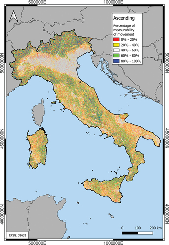
Table A4. Descending percent of measurability of movement data for the single strips.

Percentage of measurability of movement (Descending)		0% − 20%	20% − 40%	40% − 60%	60% − 80%	80% − 100%	tot [pixel]
	1d-c4_salento	25.05%	46.79%	27.41%	0.70%	0.04%	2436369
DESC_H4_01	2d-c4_puglia_calabria	26.64%	31.01%	29.44%	10.76%	2.15%	19011031
	3d-c2_foggia	27.88%	30.18%	30.73%	9.74%	1.48%	18728821
	3d-c2_sicilia_eolie	25.72%	28.77%	34.10%	10.27%	1.14%	15281814
	4d-c1_sicilia_palermo	27.25%	27.68%	34.21%	9.60%	1.26%	8006562
	4d-c4_abruzzo_campania	24.50%	27.99%	32.38%	13.07%	2.06%	14846929
	5d-c3_trieste	29.71%	33.16%	30.26%	5.42%	1.46%	1634098
	5d-c3_umbria	23.16%	26.39%	31.53%	15.17%	3.75%	24815837
	6d-c1_roma_austria	23.41%	27.02%	30.47%	14.16%	4.93%	33207873
	7d-c2_elba_austria	22.08%	22.73%	26.21%	19.56%	9.43%	28414519
	7d-c2_sardegna	24.24%	27.65%	31.82%	14.15%	2.15%	21861229
	8d-c1_liguria_svizzera	24.60%	27.04%	24.30%	16.31%	7.74%	17407608
	9d-c2_monaco_svizzera	24.49%	24.84%	25.64%	16.11%	8.93%	20533954
DESC_H4_03	1d-c3_puglia	24.73%	31.31%	43.87%	0.09%	0.00%	2849483
	2d-c3_puglia_calabria	24.51%	23.94%	34.52%	14.21%	2.83%	31357482
	3d-c3_campania_molise	24.09%	24.66%	36.56%	12.80%	1.89%	16704503
	3d-c3_sicilia_centrale	24.14%	23.46%	34.55%	16.59%	1.26%	11366632
	4d-c3_lazio	23.02%	22.12%	31.67%	18.34%	4.86%	16073733
	4d-c3_sicilia_occ	24.45%	25.67%	39.89%	8.89%	1.10%	5896800
	5d-c4_friuli	25.59%	21.21%	28.58%	15.89%	8.73%	5599280
	5d-c4_marche_roma	21.63%	22.86%	36.43%	16.01%	3.07%	23583452
	6d-c2_argent_bologna_austria	22.29%	20.97%	31.32%	18.46%	6.96%	37617263
	7d-c3_liguria_lombardia	22.41%	19.40%	26.00%	21.12%	11.07%	26113829
	7d-c3_sardegna	22.88%	24.14%	38.20%	13.16%	1.62%	22865591
	8d-c3_liguria_piemonte	23.02%	23.44%	34.95%	13.89%	4.70%	15383539
	9d-c1_valdaosta	22.85%	19.19%	22.30%	21.37%	14.29%	18344674
DESC_H4_04	1d-c2_taranto_est	27.43%	29.20%	42.67%	0.69%	0.01%	3450024
	2d-c2_sicilia_puglia	23.56%	22.34%	31.51%	18.07%	4.52%	24390331
	2d-c2_siclia_puglia_solo_sicilia	22.85%	21.44%	33.38%	15.48%	6.84%	4636002
	3d-c4_sicilia	23.41%	21.92%	31.72%	21.16%	1.80%	10084646
	3d-c4_molise_campania	22.17%	21.95%	33.19%	19.85%	2.84%	15283821
	4d-c2_centro	23.79%	21.71%	29.38%	19.48%	5.63%	21709901
	4d-c2_sicilia_ovest	23.15%	25.77%	43.38%	6.86%	0.85%	2070440
	5d-c2_roma_n_austria_new_1_north	24.22%	20.55%	29.29%	14.62%	11.31%	7407799
	5d-c2_roma_n_austria_new_2_south	20.74%	21.39%	33.99%	20.86%	3.03%	22350161
	6d-c3_toscana_trentino	21.55%	19.21%	28.31%	21.89%	9.03%	37247242
	7d-c1_liguria-svizzera	22.75%	19.39%	25.00%	21.35%	11.51%	21684241
	7d-c1_sardegna	22.29%	22.88%	37.25%	15.61%	1.96%	9001491
	8d-c2_liguria-svizzera	21.80%	19.31%	29.79%	19.12%	9.98%	25055753
	9d-c3_francia_valdaosta	20.91%	18.14%	23.41%	23.24%	14.28%	5535342
	1d-c1_calabria_new_1_puglia	27.58%	28.47%	39.59%	4.26%	0.09%	4747514
DESC_H4_05	1d-c1_calabria_new_2_calabria	21.39%	21.77%	32.78%	20.65%	3.40%	4298696
	2d-c1_catania_puglia_new_1	23.05%	22.01%	30.22%	20.57%	4.15%	18031733
	2d-c1_catania_puglia_new_2_stretto	21.82%	21.15%	33.84%	18.06%	5.13%	12610731
	3d-c1_napoli_molise	22.82%	21.77%	30.42%	21.79%	3.21%	15321372
	3d-c1_sicilia-centrale	22.57%	20.65%	28.91%	25.39%	2.48%	8930795
	4d-c1_umbria	22.24%	20.32%	27.95%	21.88%	7.59%	24419417
	5d-c1_lazio_friuli	20.95%	20.31%	31.17%	20.74%	6.83%	30789904
	6d-c4_sardegna	19.31%	18.37%	27.11%	25.03%	10.18%	10663450
	6d-c4_tirolo_elba	19.60%	17.64%	26.31%	23.74%	12.72%	34410439
	7d-c4_lombardia_liguria	23.66%	18.49%	23.82%	21.48%	12.55%	19307259
	7d-c4_sardegna	21.39%	22.85%	37.01%	16.76%	1.99%	2869025
	8d-c4_piemonte	22.05%	18.78%	27.63%	19.13%	12.40%	24724471

Figure A4. Percentage of measurability map of the Italian Peninsula, descending geometry.

Figure A5. Weighted average visibility score for the ascending tracks of H4_01.

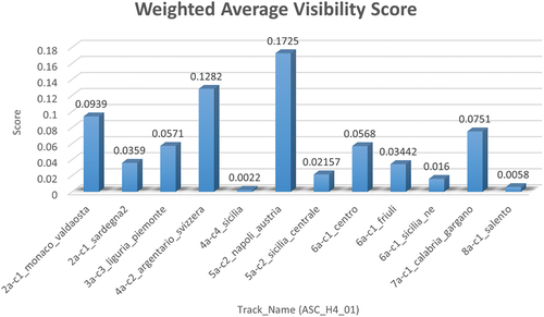
Figure A6. Weighted average visibility score for the ascending tracks of H4_03.

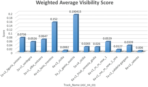
Figure A7. Weighted average visibility score for the ascending tracks of H4_04.

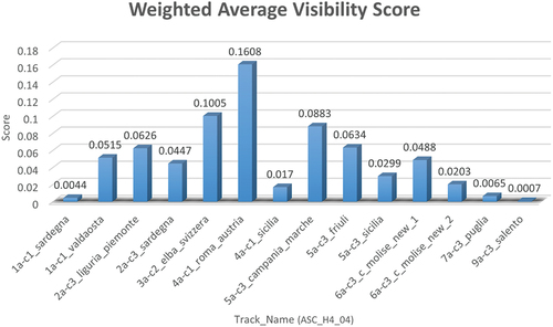
Figure A8. Weighted average visibility score for the ascending tracks of H4_05.

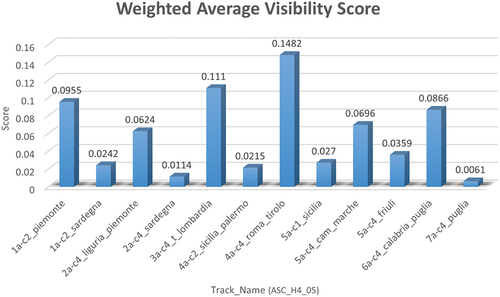
Figure A9. Weighted average visibility score for the descending tracks of H4_01.

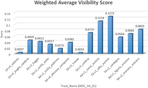
Figure A10. Weighted average visibility score for the descending tracks of H4_03.

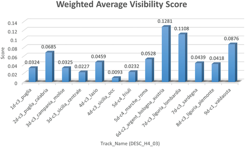
Figure A11. Weighted average visibility score for the descending tracks of H4_04.

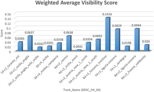
Figure A12. Weighted average visibility score for the descending tracks of H4_05.

Annex B

Figure B1. R-Index Model for ascending geometries.

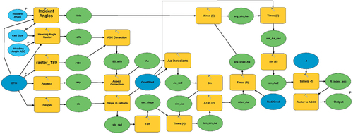
Table B1. Input and main intermediate parameters for the R-Index model in ascending geometry.

Data	Name	Description	Source
Input	DTM	Digital Terrain Model.	Italian Ministry of Environment
Input	Cell Size	Resolution of the final product.	User
Input	alfa	Heading Angle.	MapItaly Project
Input	teta	Incident Angle	8 different angles depending on the strip from the MapItaly Project (H1, H3, H4, H5)
Work	Slo	Slope obtained from the DTM.	ArcGis 10.5 Model Builder Script
Work	Asp	Aspect obtained from the DTM.	ArcGis 10.5 Model Builder Script
Work	Aa	Aspect Correction in the ascending R-Index Model.	ArcGis 10.5 Model Builder Script
Output	R_index_asc	R-Index map	ArcGis 10.5 Model Builder Script

Script B-I: Python script obtained with the ArcGis model builder for the R-Index in ascending geometry.

Table

# -*- coding: utf-8 -*- # ------------------------- # R-Index_ASC.py # Created on: 2023-11-22 19:30:10.00000

# (generated by ArcGIS/ModelBuilder) # Usage: R-Index_ASC <DTM><Cell_Size><Heading_Angle_ASC><Incident_Angle><Output>

# Description: # ------------------------- # Import arcpy module import arcpy # Script arguments DTM = arcpy.GetParameterAsText(0) Cell_Size = arcpy.GetParameterAsText(1)

Heading_Angle_ASC = arcpy.GetParameterAsText(2) Incident_Angle = arcpy.GetParameterAsText(3) Output = arcpy.GetParameterAsText(4) # Local variables: slo = ”C:\\VIS\\WORK\\slope”

Grad2Rad = ”0.0174” slo_rad = ”C:\\VIS\\WORK\\slope_rad” tan_slope = ”C:\\VIS\\WORK\\tan_slope_rad” asp = ”C:\\VIS\\WORK\\aspect”

r180 = ”C:\\VIS\\WORK\\180” alfa = ”C:\\VIS\\WORK\\alfa” v180_alfa = ”C:\\VIS\\WORK\\180_alfa” Aa = ”C:\\VIS\\WORK\\aa” Aa_rad = ”C:\\VIS\\WORK\\aa_rad”

sin_Aa = ”C:\\VIS\\WORK\\sin_aa” tan_sin_Aa = ”C:\\VIS\\WORK\\tan_sin_aa” Atan_Aa = ”C:\\VIS\\WORK\\atan_aa” Rad2Grad = ”57.29”

arg_grad_Aa = ”C:\\VIS\\WORK\\arg_grad_aa” teta = ”C:\\VIS\\WORK\\teta” arg_sin_Aa = ”C:\\VIS\\WORK\\arg_sin_Aa”

sin_Aa_rad = ”C:\\VIS\\WORK\\sin_aa_rad” sin_Aa2 = ”C:\\VIS\\WORK\\sin_aa2” v_1 = ”-1” R_index_asc = ”C:\\VIS\\WORK\\R_index_asc”

# Process: Slope arcpy.Slope_3d(DTM, slo, ”DEGREE”, ”1”) # Process: Slope in radians arcpy.gp.Times_sa(slo, Grad2Rad, slo_rad) # Process: Tan arcpy.gp.Tan_sa(slo_rad, tan_slope) # Process: Aspect arcpy.Aspect_3d(DTM, asp) # Process: raster_180

arcpy.gp.CreateConstantRaster_sa(r180, ”180”, ”FLOAT”, ”10”, DTM) # Process: Heading Angle Raster arcpy.gp.CreateConstantRaster_sa(alfa, Heading_Angle_ASC, ”FLOAT”, Cell_Size, DTM)

# Process: ASC Correction arcpy.gp.Plus_sa(r180, alfa, v180_alfa) # Process: Aspect Correction arcpy.gp.Plus_sa(asp, v180_alfa, Aa) # Process: Aa in radians

arcpy.gp.Times_sa(Aa, Grad2Rad, Aa_rad) # Process: Sin arcpy.gp.Sin_sa(Aa_rad, sin_Aa) # Process: Times (4) arcpy.gp.Times_sa(tan_slope, sin_Aa, tan_sin_Aa) # Process: ATan (2) arcpy.gp.ATan_sa(tan_sin_Aa, Atan_Aa) # Process: Times (9) arcpy.gp.Times_sa(Atan_Aa, Rad2Grad, arg_grad_Aa)

# Process: Incident Angles Raster arcpy.gp.CreateConstantRaster_sa(teta, Incident_Angle, ”FLOAT”, Cell_Size, DTM) # Process: Minus (5) arcpy.gp.Minus_sa(arg_grad_Aa, teta, arg_sin_Aa) # Process: Times (5) arcpy.gp.Times_sa(arg_sin_Aa, Grad2Rad, sin_Aa_rad) # Process: Sin (6)

arcpy.gp.Sin_sa(sin_Aa_rad, sin_Aa2) # Process: Times -1 arcpy.gp.Times_sa(sin_Aa2, v_1, R_index_asc) # Process: Raster to ASCII arcpy.RasterToASCII_conversion(R_index_asc, Output)

Figure B2. R-Index Model for descending geometries.

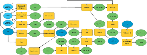
Table B2. Input and main intermediate parameters for the R-Index model in ascending geometry.

Data	Name	Description	Source
Input	DTM	Digital Terrain Model.	Italian Ministry of Environment
Input	Cell Size	Resolution of the final product.	User
Input	alfa	Heading Angle.	MapItaly Project
Input	teta	Incident Angle.	8 different angles depending on the strip from the MapItaly Project (H1, H3, H4, H5)
Work	Slo	Slope obtained from the DTM.	ArcGis 10.5 Model Builder Script
Work	Asp	Aspect obtained from the DTM.	ArcGis 10.5 Model Builder Script
Work	Ad	Aspect Correction in the descending R-Index Model.	ArcGis 10.5 Model Builder Script
Output	R_index_desc	R-Index map.	ArcGis 10.5 Model Builder Script

Script B-II: Python script obtained with the ArcGis model builder for the R-Index in descending geometry.

Table

# -*- coding: utf-8 -*- # ------------------------- # R-Index_DSC.py # Created on: 2023-11-22 18:59:02.00000

# (generated by ArcGIS/ModelBuilder) # Usage: R-Index_DSC <DTM><Cell_Size><Heading_Angle_DSC><Incident_Angle_DSC><Output> # Description: # -------------------------

# Import arcpy module import arcpy # Script arguments DTM = arcpy.GetParameterAsText(0) Cell_Size = arcpy.GetParameterAsText(1) Heading_Angle_DSC = arcpy.GetParameterAsText(2) Incident_Angle_DSC = arcpy.GetParameterAsText(3)

Output = arcpy.GetParameterAsText(4) # Local variables: asp = “C:\\VIS\\WORK\\aspect” alfa = “C:\\VIS\\WORK\\alfa” r180 = “C:\\VIS\\WORK\\180” v180_alfa = “C:\\Users\\giuse\\OneDrive\\Documenti\\ArcGIS\\Default1.gdb\\Minus_alfa1”

Ad = “C:\\VIS\\WORK\\ad” Grad2Rad = “0.0174” Ad_rad = “C:\\VIS\\WORK\\ad_rad” sin_Ad = “C:\\VIS\\WORK\\sin_ad” slo = “C:\\VIS\\WORK\\slope” slo_rad = “C:\\VIS\\WORK\\slope_rad”

tan_slope = “C:\\VIS\\WORK\\tan_slope_rad” tan_sin_Ad = “C:\\VIS\\WORK\\tan_sin_ad” Atan_Ad = “C:\\VIS\\WORK\\atan_ad” Rad2Grad = “57.29”

arg_grad_Ad = “C:\\VIS\\WORK\\arg_grad_ad” teta = “C:\\VIS\\WORK\\teta” arg_sin_Ad = “C:\\VIS\\WORK\\arg_sin_ad” sin_Ad_rad = “C:\\VIS\\WORK\\sin_ad_rad”

sin_Ad2 = “C:\\VIS\\WORK\\sin_ad2” v_1 = “-1” R_index_desc = “C:\\VIS\\WORK\\R_index_desc” # Process: Aspect arcpy.Aspect_3d(DTM, asp) # Process: Angle from North Raster

arcpy.gp.CreateConstantRaster_sa(alfa, Heading_Angle_DSC, “FLOAT”, Cell_Size, DTM) # Process: raster_180 arcpy.gp.CreateConstantRaster_sa(r180, “180”, “FLOAT”, “10”, DTM) # Process: DSC Correction

arcpy.gp.Minus_sa(alfa, r180, v180_alfa) # Process: Aspect Correction arcpy.gp.Minus_sa(asp, v180_alfa, Ad) # Process: Ad in radians arcpy.gp.Times_sa(Ad, Grad2Rad, Ad_rad) # Process: Sin

arcpy.gp.Sin_sa(Ad_rad, sin_Ad) # Process: Slope arcpy.Slope_3d(DTM, slo, “DEGREE”, “1”) # Process: Slope in radians arcpy.gp.Times_sa(slo, Grad2Rad, slo_rad) # Process: Tan

arcpy.gp.Tan_sa(slo_rad, tan_slope) # Process: Times (7) arcpy.gp.Times_sa(sin_Ad, tan_slope, tan_sin_Ad) # Process: ATan arcpy.gp.ATan_sa(tan_sin_Ad, Atan_Ad)

# Process: Times (3) arcpy.gp.Times_sa(Atan_Ad, Rad2Grad, arg_grad_Ad) # Process: Incident Angles arcpy.gp.CreateConstantRaster_sa(teta, Incident_Angle_DSC, “FLOAT”, Cell_Size, DTM) # Process: Minus (4) arcpy.gp.Minus_sa(arg_grad_Ad, teta, arg_sin_Ad) # Process: Times (8)

arcpy.gp.Times_sa(arg_sin_Ad, Grad2Rad, sin_Ad_rad) # Process: Sin (5) arcpy.gp.Sin_sa(sin_Ad_rad, sin_Ad2)

# Process: Times -1 arcpy.gp.Times_sa(sin_Ad2, v_1, R_index_desc) # Process: Raster to ASCII arcpy.RasterToASCII_conversion(R_index_desc, Output)

Figure B3. Percentage of movement measurability Model for ascending geometries.

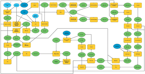
Table B3. Input and main intermediate parameters for the percentage of movement measurability model in ascending geometry.

Data	Name	Description	Source
Input	DTM	Digital Terrain Model.	Italian Ministry of Environment
Input	Cell Size	Resolution of the final product.	User
Input	epsilon	Heading Angle.	MapItaly Project
Input	teta	Incident Angle.	8 different angles depending on the strip from the MapItaly Project (H1, H3, H4, H5) and the geometry (ASC or DSC)
Work	Slo	Slope obtained from the DTM.	ArcGis 10.5 Model Builder Script
Work	Asp	Aspect obtained from the DTM.	ArcGis 10.5 Model Builder Script
Work	Beta	(90°-Asp)+Epsilon	ArcGis 10.5 Model Builder Script
Work	Abs_xh_asc	Absolute value of the cosine of Beta. |cos(Beta)|	ArcGis 10.5 Model Builder Script
Work	x_v_aver	Component of the Percentage for the slopes facing the satellite.	ArcGis 10.5 Model Builder Script
Work	x_v_tow	Component of the Percentage for the slopes facing away from the satellite.	ArcGis 10.5 Model Builder Script
Work	x_v_asc	Mosaic of the two elements. x_v_aver + x_v_tow	ArcGis 10.5 Model Builder Script
Output	x_tot_asc	Percentage of Measurability of Movement map.	ArcGis 10.5 Model Builder Script

Figure B4. Percentage of movement Model for descending geometries.

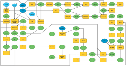
Script B-III: Python script obtained with the ArcGis model builder for the Percentage of measurability of movement in ascending geometry.

Table

# -*- coding: utf-8 -*- # ------------------------- # PER_ASC.py # Created on: 2023-09-29 18:49:40.00000 # (generated by ArcGIS/ModelBuilder) # Usage: PER_ASC <DEM> <Cell_size> <Heading_Angle> <Incident_Angle> <Output>

# Description: # ------------------------- # Import arcpy module import arcpy # Script arguments DEM = arcpy.GetParameterAsText(0) if DEM == ‘#’ or not DEM: DEM = “DEM_2A-C1_Monaco_Valdaosta.tif” # Provide a default value if unspecified

Cell_size = arcpy.GetParameterAsText(1) if Cell_size == ‘#’ or not Cell_size: Cell_size = “10” # Provide a default value if unspecified Heading_Angle = arcpy.GetParameterAsText(2)

if Heading_Angle == ‘#’ or not Heading_Angle: Heading_Angle = “-10” # Provide a default value if unspecified Incident_Angle = arcpy.GetParameterAsText(3) if Incident_Angle == ‘#’ or not Incident_Angle: Incident_Angle = “26.65” # Provide a default value if unspecified

Output = arcpy.GetParameterAsText(4) if Output == ‘#’ or not Output: Output = “C:\\VIS\\OUTPUT\\NAME_PERC_ASC.asc” # Provide a default value if unspecified # Local variables: r90 = “C:\\VIS\\WORK\\r90”

Grad2Rad = “0.0174” r90_rad = “C:\\VIS\\WORK\\90_rad” asp = “C:\\VIS\\WORK\\asp” asp_rad = “C:\\VIS\\WORK\\asp_rad” r90_rad_asp_rad = “C:\\VIS\\WORK\\90-asp_rad”

epsilon = “C:\\VIS\\WORK\\epsilon” epsilon_rad = “C:\\VIS\\WORK\\epsilon_rad” beta = “C:\\VIS\\WORK\\beta” cos_beta = “C:\\VIS\\WORK\\cos_beta” abs_xh_asc = “C:\\VIS\\WORK\\abs_xh_asc”

rIncAng = “C:\\VIS\\WORK\\HA” r90_rIA = “C:\\VIS\\WORK\\r90-rHA” slo = “C:\\VIS\\WORK\\slope” asp_int = “C:\\VIS\\WORK\\asp_int” asp_east = “C:\\VIS\\WORK\\asp_east” slope_east = “C:\\VIS\\WORK\\slope_east”

slope_east_r = “C:\\VIS\\WORK\\slope_east_r” tan_east = “C:\\VIS\\WORK\\tan_east” delta_east = “C:\\VIS\\WORK\\delta_east” atan_east = “C:\\VIS\\WORK\\atan_east”

Rad2Grad = “57.296” delta_e_grad = “C:\\VIS\\WORK\\delta_e_grad” ro_east = “C:\\VIS\\WORK\\ro_east” ro_east_rad = “C:\\VIS\\WORK\\ro_east_rad”

x_v_aver = “C:\\VIS\\WORK\\x_v_aver” x_v_asc = x_v_aver asp_west = “C:\\VIS\\WORK\\asp_west” slope_west = “C:\\VIS\\WORK\\slope_west” slope_west_r = “C:\\VIS\\WORK\\slope_west_r”

tan_west = “C:\\VIS\\WORK\\tan_west” delta_west = “C:\\VIS\\WORK\\delta_west” atan_west = “C:\\VIS\\WORK\\atan_west” delta_w_grad = “C:\\VIS\\WORK\\delta_w_grad” ro_west = “C:\\VIS\\WORK\\ro_west”

ro_west_rad = “C:\\VIS\\WORK\\ro_west_rad” x_v_tow = “C:\\VIS\\WORK\\x_v_tow” WORK = “C:\\VIS\\WORK” x_tot_asc = “C:\\VIS\\WORK\\x_tot_asc”

# Process: Create Constant Raster arcpy.gp.CreateConstantRaster_sa(r90, “90”, “FLOAT”, Cell_size, DEM) # Process: r90 in Radiants arcpy.gp.Times_sa(r90, Grad2Rad, r90_rad) # Process: Aspect arcpy.Aspect_3d(DEM, asp) # Process: Aspect in Radiants

arcpy.gp.Times_sa(asp, Grad2Rad, asp_rad) # Process: Minus arcpy.gp.Minus_sa(r90_rad, asp_rad, r90_rad_asp_rad) # Process: Heading Angle Epsilon arcpy.gp.CreateConstantRaster_sa(epsilon, Heading_Angle, “FLOAT”, Cell_size, DEM)

# Process: Epsilon in Radiants arcpy.gp.Times_sa(epsilon, Grad2Rad, epsilon_rad) # Process: Plus (2) arcpy.gp.Plus_sa(r90_rad_asp_rad, epsilon_rad, beta) # Process: Cos arcpy.gp.Cos_sa(beta, cos_beta) # Process: Abs

arcpy.gp.Abs_sa(cos_beta, abs_xh_asc) # Process: r_IA arcpy.gp.CreateConstantRaster_sa(rIncAng, Incident_Angle, “FLOAT”, Cell_size, DEM) # Process: Minus (2) arcpy.gp.Minus_sa(r90, rIncAng, r90_rIA) # Process: Slope

arcpy.Slope_3d(DEM, slo, “DEGREE”, “1”) # Process: Aspect in Integers arcpy.gp.Int_sa(asp, asp_int) # Process: Extraction of the East facing data

arcpy.gp.ExtractByAttributes_sa(asp_int, “VALUE >=0 AND VALUE <=170 OR VALUE >=350 AND VALUE <360”, asp_east) # Process: East facing Slopes arcpy.gp.ExtractByMask_sa(slo, asp_east, slope_east) # Process: East-facing slopes in radiants

arcpy.gp.Times_sa(slope_east, Grad2Rad, slope_east_r) # Process: Tan east arcpy.gp.Tan_sa(slope_east_r, tan_east) # Process: Times (6) arcpy.gp.Times_sa(tan_east, cos_beta, delta_east) # Process: ATan delta east

arcpy.gp.ATan_sa(delta_east, atan_east) # Process: Times (9) arcpy.gp.Times_sa(atan_east, Rad2Grad, delta_e_grad) # Process: Minus (3)

arcpy.gp.Minus_sa(r90_rIA, delta_e_grad, ro_east) # Process: Times (11) arcpy.gp.Times_sa(ro_east, Grad2Rad, ro_east_rad) # Process: Cos (2) arcpy.gp.Cos_sa(ro_east_rad, x_v_aver)

# Process: Extraction of the West facing data arcpy.gp.ExtractByAttributes_sa(asp_int, “\VALUE\” > 170 AND “\VALUE\” <= 350”, asp_west) # Process: West facing Slopes

arcpy.gp.ExtractByMask_sa(slo, asp_west, slope_west) # Process: West-facing slopes in radiants arcpy.gp.Times_sa(slope_west, Grad2Rad, slope_west_r)

# Process: Tan west arcpy.gp.Tan_sa(slope_west_r, tan_west) # Process: Times (7) arcpy.gp.Times_sa(tan_west, cos_beta, delta_west) # Process: Atan Delta west

arcpy.gp.ATan_sa(delta_west, atan_west) # Process: Times (10) arcpy.gp.Times_sa(atan_west, Rad2Grad, delta_w_grad) # Process: Plus

arcpy.gp.Plus_sa(delta_w_grad, r90_rIA, ro_west) # Process: Times (12) arcpy.gp.Times_sa(ro_west, Grad2Rad, ro_west_rad) # Process: Cos (3)

arcpy.gp.Cos_sa(ro_west_rad, x_v_tow) # Process: Mosaic To New Raster arcpy.MosaicToNewRaster_management(“C:\\VIS\\WORK\\x_v_aver;C:\\VIS\\WORK\\x_v_tow”, WORK, “x_v_asc”, “”, “8_BIT_UNSIGNED”, “”, “1”, “LAST”, “FIRST”) # Process: Times (13)

arcpy.gp.Times_sa(abs_xh_asc, x_v_asc, x_tot_asc) # Process: Raster to ASCII arcpy.RasterToASCII_conversion(x_tot_asc, Output)

Table B4. Input and main intermediate parameters for the percentage of movement measurability model in ascending geometry.

Data	Name	Description	Source
Input	DTM	Digital Terrain Model.	Italian Ministry of Environment
Input	Cell Size	Resolution of the final product.	User
Input	epsilon	Heading Angle.	MapItaly Project
Input	teta	Incident Angle.	8 different angles depending on the strip from the MapItaly Project (H1, H3, H4, H5) and the geometry (ASC or DSC)
Work	Slo	Slope obtained from the DTM.	ArcGis 10.5 Model Builder Script
Work	Asp	Aspect obtained from the DTM.	ArcGis 10.5 Model Builder Script
Work	Beta	(90°-Asp)+Epsilon	ArcGis 10.5 Model Builder Script
Work	Abs_xh_desc	Absolute value of the cosine of Beta. |cos(Beta)|	ArcGis 10.5 Model Builder Script
Work	x_v_aver	Component of the Percentage for the slopes facing the satellite.	ArcGis 10.5 Model Builder Script
Work	x_v_tow	Component of the Percentage for the slopes facing away from the satellite.	ArcGis 10.5 Model Builder Script
Work	x_v_desc	Mosaic of the two elements. x_v_aver + x_v_tow	ArcGis 10.5 Model Builder Script
Output	x_tot_desc	Percentage of Measurability of Movement map.	ArcGis 10.5 Model Builder Script

Script B-IV: Python script obtained with the ArcGis model builder for the Percentage of measurability of movement in ascending geometry.

Table

# -*- coding: utf-8 -*- #------------------------- # %_DSC.py # Created on: 2023-11-22 20:55:48.00000 #   (generatedby ArcGIS/ModelBuilder)

# Usage: %_DSC <DTM><Cell_Size><Heading_Angle_DSC><Incident_Angle_DSC><Output> # Description: #-------------------------

# Import arcpy module import arcpy # Script arguments DTM = arcpy.GetParameterAsText(0) Cell_Size = arcpy.GetParameterAsText(1)

Heading_Angle_DSC = arcpy.GetParameterAsText(2) Incident_Angle_DSC = arcpy.GetParameterAsText(3) Output = arcpy.GetParameterAsText(4) # Local variables: r90 = ”C:\\VIS\\WORK\\r90” Grad2Rad = ”0.0174”

r90_rad = ”C:\\VIS\\WORK\\90_rad” asp = ”C:\\VIS\\WORK\\aspect” asp_rad = ”C:\\VIS\\WORK\\asp_rad” r90_rad_asp_rad = ”C:\\VIS\\WORK\\90-asp_rad”

epsilon = ”C:\\VIS\\WORK\\epsilon” epsilon_rad = ”C:\\VIS\\WORK\\epsilon_rad” beta = ”C:\\VIS\\WORK\\beta2” cos_beta = ”C:\\VIS\\WORK\\cos_beta” abs_xh_desc = ”C:\\VIS\\WORK\\abs_xh_desc”

slo = ”C:\\VIS\\WORK\\slope” asp_int = ”C:\\VIS\\WORK\\asp_int” asp_east = ”C:\\VIS\\WORK\\asp_east” slope_east = ”C:\\VIS\\WORK\\slope_east” slope_e_rad = ”C:\\VIS\\WORK\\slope_e_rad”

tan_east = ”C:\\VIS\\WORK\\tan_east” delta_east = ”C:\\VIS\\WORK\\delta_east” atan_east = ”C:\\VIS\\WORK\\atan_east” Rad2Grad = ”57.296”

delta_e_grad= ”C:\\VIS\\WORK\\delta_e_grad” rInc_Ang = ”C:\\VIS\\WORK\\r_IA” r90_IA = ”C:\\VIS\\WORK\\r90-IA” ro_east = ”C:\\VIS\\WORK\\ro_east” ro_east_rad = ”C:\\VIS\\WORK\\ro_east_rad”

x_v_tow = ”C:\\VIS\\WORK\\x_v_tow” x_v_desc = x_v_tow asp_west = ”C:\\VIS\\WORK\\asp_west” slope_west = ”C:\\VIS\\WORK\\slope_west” slope_w_rad = ”C:\\VIS\\WORK\\slope_w_rad”

tan_west = ”C:\\VIS\\WORK\\tan_west” delta_west = ”C:\\VIS\\WORK\\delta_west” atan_west = ”C:\\VIS\\WORK\\atan_west” delta_w_grad = ”C:\\VIS\\WORK\\delta_w_grad” ro_west = ”C:\\VIS\\WORK\\ro_west”

ro_west_rad = ”C:\\VIS\\WORK\\ro_west_rad” x_v_aver = ”C:\\VIS\\WORK\\x_v_aver” Composed_Empty_Raster = ”C:\\VIS\\WORK” x_tot_desc = ”C:\\VIS\\WORK\\x_tot_desc” # Process: Create Constant Raster

arcpy.gp.CreateConstantRaster_sa(r90, ”90”,”FLOAT”, Cell_Size, DTM) # Process: r90 in Radiants arcpy.gp.Times_sa(r90, Grad2Rad, r90_rad) # Process: Aspect arcpy.Aspect_3d(DTM, asp) # Process: Aspect in Radiants

arcpy.gp.Times_sa(asp, Grad2Rad, asp_rad) # Process: Minus arcpy.gp.Minus_sa(r90_rad, asp_rad, r90_rad_asp_rad) # Process: Heading Angle Epsilon arcpy.gp.CreateConstantRaster_sa(epsilon,Heading_Angle_DSC, ”FLOAT”, ”10”, DTM) # Process: Epsilon in radians arcpy.gp.Times_sa(epsilon, Grad2Rad, epsilon_rad)

# Process: Plus (2) arcpy.gp.Plus_sa(r90_rad_asp_rad, epsilon_rad, beta) # Process: Cos arcpy.gp.Cos_sa(beta, cos_beta) # Process: Abs arcpy.gp.Abs_sa(cos_beta, abs_xh_desc) # Process: Slope arcpy.Slope_3d(DTM, slo, ”DEGREE”,”1”) # Process: Aspect in Integers arcpy.gp.Int_sa(asp, asp_int) # Process: Extraction of the East facing data

arcpy.gp.ExtractByAttributes_sa(asp_int, ”VALUE>=0 AND VALUE <=170 OR VALUE >350 AND VALUE <=360”, asp_east) # Process: East facing Slopes arcpy.gp.ExtractByMask_sa(slo, asp_east, slope_east) # Process: east facing slopes in radians

arcpy.gp.Times_sa(slope_east, Grad2Rad, slope_e_rad) # Process: Tan arcpy.gp.Tan_sa(slope_e_rad, tan_east) # Process: Times (6) arcpy.gp.Times_sa(tan_east, cos_beta, delta_east) # Process: ATan arcpy.gp.ATan_sa(delta_east, atan_east)

# Process: Times (9) arcpy.gp.Times_sa(atan_east, Rad2Grad, delta_e_grad) # Process: Create Constant Raster (2) arcpy.gp.CreateConstantRaster_sa(rInc_Ang,Incident_Angle_DSC, ”FLOAT”, Cell_Size, DTM) # Process: Minus (3) arcpy.gp.Minus_sa(r90, rInc_Ang, r90_IA)

# Process: Plus (3) arcpy.gp.Plus_sa(delta_e_grad, r90_IA, ro_east) # Process: Times (11) arcpy.gp.Times_sa(ro_east, Grad2Rad, ro_east_rad) # Process: Cos (2) arcpy.gp.Cos_sa(ro_east_rad, x_v_tow) # Process: Extraction of the West facing data

arcpy.gp.ExtractByAttributes_sa(asp_int, ”VALUE>170 AND VALUE <=350”, asp_west) # Process: West facing Slopes arcpy.gp.ExtractByMask_sa(slo, asp_west, slope_west) # Process: Times (5) arcpy.gp.Times_sa(slope_west, Grad2Rad, slope_w_rad) # Process: Tan (2)

arcpy.gp.Tan_sa(slope_w_rad, tan_west) # Process: Times (7) arcpy.gp.Times_sa(tan_west, cos_beta, delta_west) # Process: ATan (2) arcpy.gp.ATan_sa(delta_west, atan_west) # Process: Times (10) arcpy.gp.Times_sa(atan_west, Rad2Grad, delta_w_grad) # Process: Minus (2) arcpy.gp.Minus_sa(r90_IA, delta_w_grad, ro_west) # Process: Times (12)

arcpy.gp.Times_sa(ro_west, Grad2Rad, ro_west_rad) # Process: Cos (3) arcpy.gp.Cos_sa(ro_west_rad, x_v_aver) # Process: Mosaic To New Raster arcpy.MosaicToNewRaster_management(”C:\\VIS\\WORK\\x_v_tow;C:\\VIS\\WORK\\x_v_aver”,Composed_Empty_Raster, ”x_v_desc”, ””,”32_BIT_FLOAT”, ””, ”1”, ”LAST”,”FIRST”)

# Process: Times (13) arcpy.gp.Times_sa(abs_xh_desc, x_v_desc, x_tot_desc) # Process: Raster to ASCII arcpy.RasterToASCII_conversion(x_tot_desc, Output)

References

- Ammirati, L., N. Mondillo, R. A. Rodas, C. Sellers, and D. Di Martire. 2020. “Monitoring Land Surface Deformation Associated with Gold Artisanal Mining in the Zaruma City (Ecuador).” Remote Sensing 12 (13): 2135. https://doi.org/10.3390/rs12132135.
- Battagliere, M. L., M. Virelli, F. Lenti, D. Lauretta, and A. Coletta. 2019. “A Review of the Exploitation of the Operational Mission COSMO-Skymed: Global Trends (2014-2017).” Space Policy 48 (May 1): 60–45. https://doi.org/10.1016/j.spacepol.2019.01.003.
- Boni, G., L. Ferraris, L. Pulvirenti, G. Squicciarino, N. Pierdicca, L. Candela, A. R. Pisani, et al. 2016. “A Prototype System for Flood Monitoring Based on Flood Forecast Combined with COSMO-Skymed and Sentinel-1 Data.” IEEE Journal of Selected Topics in Applied Earth Observations & Remote Sensing 9 (6): 2794–2805. https://doi.org/10.1109/JSTARS.2016.2514402.
- Bovenga, F., L. Candela, F. Casu, G. Fornaro, F. Guzzetti, R. Lanari, D. O. Nitti, R. Nutricato, and D. Reale. 2010. The COSMO SkyMed Constellation Turn on the l’Aquila Earthquake: DInSAR Results of the MORFEO Project. In 2010 IEEE International Geoscience and Remote Sensing Symposium, Honolulu, HI, USA, 4803–4806. IEEE.
- Bovenga, F., J. Wasowski, D. O. Nitti, R. Nutricato, and M. T. Chiaradia. 2012. “Using COSMO/SkyMed X-Band and ENVISAT C-Band SAR Interferometry for Landslides Analysis.” Remote Sensing of Environment 119:272–285. https://doi.org/10.1016/j.rse.2011.12.013.
- Caló, F., D. Notti, J. P. Galve, S. Abdikan, T. Görüm, A. Pepe, and F. Balik Şanli. 2017. “DInSAR-Based Detection of Land Subsidence and Correlation with Groundwater Depletion in Konya Plain, Turkey.” Remote Sensing 9 (1): 83. https://doi.org/10.3390/rs9010083.
- Caltagirone, F., G. De Luca, F. Covello, G. Marano, G. Angino, and M. Piemontese. 2010. Status, Results, Potentiality and Evolution of COSMO-Skymed, the Italian Earth Observation Constellation for Risk Management and Security. In 2010 IEEE International Geoscience and Remote Sensing Symposium, Honolulu, HI, USA, 4393–4396.
- Carnemolla, F., G. De Guidi, A. Bondorte, F. Brighenti, and P. Briole. 2023. “The Ground Deformation of the South-Eastern Flank of Mount Etna Monitored by GNSS and SAR Interferometry from 2016 to 2019.” Geophysical Journal International 234 (1): 664–682. https://doi.org/10.1093/gji/ggad088.
- Chini, M., L. Pulvirenti, and N. Pierdicca. 2012. “Analysis and Interpretation of the COSMO-Skymed Observations of the 2011 Japan Tsunami.” IEEE Geoscience and Remote Sensing Letters 9 (3): 467–471. https://doi.org/10.1109/LGRS.2011.2182495.
- Ciappa, A., L. Pietranera, and F. Battazza. 2010. “Perito Moreno Glacier (Argentina) Flow Estimation by COSMO SkyMed Sequence of High-Resolution SAR-X Imagery.” Remote Sensing of Environment 114 (9): 2088–2096. ISSN 0034-4257. https://doi.org/10.1016/j.rse.2010.04.014.
- Ciervo, F., G. Rianna, P. Mercogliano, and M. N. Papa. 2017. “Effects of Climate Change on Shallow Landslides in a Small Coastal Catchment in Southern Italy.” Landslides 14 (3): 1043–1055. https://doi.org/10.1007/s10346-016-0743-1.
- Cigna, F., R. Lasaponara, N. Masini, P. Milillo, and D. Tapete. 2014. “Persistent Scatterer Interferometry Processing of COSMO-Skymed StripMap HIMAGE Time Series to Depict Deformation of the Historic Centre of Rome, Italy.” Remote Sensing 6 (12): 12593–12618. https://doi.org/10.3390/rs61212593.
- Colesanti, C., and J. Wasowski. 2006. “Investigating Landslides with Space-Borne Synthetic Aperture Radar (SAR) Interferometry.” Engineering Geology 88 (3): 173–199. https://doi.org/10.1016/j.enggeo.2006.09.013.
- Confuorto, P., D. Di Martire, G. Centolanza, R. Iglesias, J. J. Mallorqui, A. Novellino, S. Plank, M. Ramondini, K. Thuro, and D. Calcaterra. 2017. “Post-Failure Evolution Analysis of a Rainfall-Triggered Landslide by Multi-Temporal Interferometry SAR Approaches Integrated with Geotechnical Analysis.” Remote Sensing of Environment 188 (1), (January): 51–72. https://doi.org/10.1016/j.rse.2016.11.002.
- Costabile, S. 2010. “The National Geoportal: The Not-Ordinary Plan of Environmental Remote Sensing (In Italian).” GEOmedia 14:3.
- Costantini, M., J. Bai, F. Malvarosa, F. Minati, F. Vecchioli, R. Wang, Q. Hu, J. Xiao, and J. Li. 2016. Ground Deformations and Building Stability Monitoring by COSMO-Skymed PSP SAR Interferometry: Results and Validation with Field Measurements and Surveys. In 2016 IEEE International Geoscience and Remote Sensing Symposium (IGARSS), Beijing, China, 6847–6850. IEEE.
- Costantini, M., A. Ferretti, F. Minati, S. Falco, F. Trillo, D. Colombo, F. Novali, et al. 2017. “Analysis of Surface Deformations Over the Whole Italian Territory by Interferometric Processing of ERS, Envisat and COSMO-Skymed Radar Data.” Remote Sensing of Environment 202:250–275. December 1. https://doi.org/10.1016/j.rse.2017.07.017. Big Remotely Sensed Data: Tools, Applications and Experiences.
- Costantini, M., F. Malvarosa, F. Minati, and F. Vecchioli. 2012. Multi-Scale and Block Decomposition Methods for Finite Difference Integration and Phase Unwrapping of Very Large Datasets in High Resolution SAR Interferometry. In 2012 IEEE International Geoscience and Remote Sensing Symposium, Munich, Germany, 5574–5577. IEEE.
- Costantini, M., F. Minati, F. Trillo, A. Ferretti, E. Passera, A. Rucci, J. Dehls. 2022. EGMS: Europe-Wide Ground Motion Monitoring Based on Full Resolution Insar Processing of All Sentinel-1 Acquisitions. In IGARSS 2022 - 2022 IEEE International Geoscience and Remote Sensing Symposium, Kuala Lumpur, Malaysia, 5093–5096.
- Covello, F., F. Battazza, A. Coletta, E. Lopinto, C. Fiorentino, L. Pietranera, G. Valentini, and S. Zoffoli. 2010. “COSMO-Skymed an Existing Opportunity for Observing the Earth.” Journal of Geodynamics Volume 49 (3–4): 171–180. ISSN 0264-3707. https://doi.org/10.1016/j.jog.2010.01.001.
- Crosetto, M., O. Monserrat, R. Iglesias, and B. Crippa. 2010. “Persistent Scatterer Interferometry.” Photogrammetric Engineering & Remote Sensing 76 (no. 9), (September 1): 1061–1069. https://doi.org/10.14358/PERS.76.9.1061.
- Del Soldato, M., L. Solari, A. Novellino, O. Monserrat, and F. Raspini. 2021. “A New Set of Tools for the Generation of InSAR Visibility Maps Over Wide Areas.” Geosciences 2021 (6): 11, 229. https://doi.org/10.3390/geosciences11060229.
- Dey, T. K., K. Biswas, D. Chakravarty, A. Misra, and B. Samanta. 2019. Spatio-Temporal Subsidence Estimation of Jharia Coal Field, India Using SBAS-Dinsar with Cosmo-Skymed Data. In IGARSS 2019-2019 IEEE International Geoscience and Remote Sensing Symposium, Yokohama, Japan, 2123–2126. IEEE.
- Di Martire, D., M. Paci, P. Confuorto, S. Costabile, F. Gustaferro, A. Verta, and D. Calcaterra 2017. “A Nation-Wide System for Landslide Mapping and Risk Management in Italy: The Second Not-Ordinary Plan of Environmental Remote Sensing.” International Journal of Applied Earth Observation and Geoinformation 63:143–157. https://doi.org/10.1016/j.jag.2017.07.018.
- Di Napoli, M., D. Di Martire, G. Bausilio, D. Calcaterra, P. Confuorto, M. Firpo, G. Pepe, and A. Cevasco. 2021. “Rainfall-Induced Shallow Landslide Detachment, Transit and Runout Susceptibility Mapping by Integrating Machine Learning Techniques and GIS-Based Approaches.” Water 13 (4): 488. https://doi.org/10.3390/w13040488.
- Duro, J., D. Albiol, O. Mora, and B. Payàs, 2013. Application of Advanced InSAR Techniques for the Measurement of Vertical and Horizontal Ground Motion in Longwall Minings. Resource Operators Conference (January 1). https://ro.uow.edu.au/coal/442.
- Esposito, C., N. Belcecchi, F. Bozzano, A. Brunetti, G. M. Marmoni, P. Mazzanti, S. Romeo, F. Cammillozzi, G. Cecchini, and M. Spizzirri. 2021. “Integration of Satellite-Based A-DInSAR and Geological Modeling Supporting the Prevention from Anthropogenic Sinkholes: A Case Study in the Urban Area of Rome.” Geomatics, Natural Hazards and Risk 12 (no. 1), (January 1): 2835–2864. https://doi.org/10.1080/19475705.2021.1978562.
- ESRI Inc. 2016. ArcMap (Version 10.5). Environmental Systems Research Institute.
- Ferretti, A., C. Prati, and F. Rocca. 2001. “Permanent scatterers in SAR interferometry.” IEEE Transactions on Geoscience and Remote Sensing 39 (1): 8–20. https://doi.org/10.1109/36.898661.
- Fielding, E. J., M. Simons, S. Owen, P. Lundgren, H. Hua, P. Agram, Z. Liu, et al. 2014. “Rapid Imaging of Earthquake Ruptures with Combined Geodetic and Seismic Analysis.” Procedia Technology 16:876–885. https://doi.org/10.1016/j.protcy.2014.10.038.
- Franceschetti, G., and R. Lanari. 1999. Synthetic Aperture Radar Processing. Boca Raton: CRC Press.
- Fusco, F., R. Tufano, P. De Vita, D. Di Martire, M. Di Napoli, L. Guerriero, F. A. Mileti, F. Terribile, and D. Calcaterra. 2023. “A Revised Landslide Inventory of the Campania Region (Italy).” Scientific Data 10 (1): 355. https://doi.org/10.1038/s41597-023-02155-6.
- Galve, J. P., C. Castañeda, F. Gutiérrez, and G. Herrera. 2015. “Assessing Sinkhole Activity in the Ebro Valley Mantled Evaporite Karst Using Advanced DInSAR. Geomorphology 229.” Karst Geomorphology: From Hydrological Functioning to Palaeoenvironmental Reconstructions (January 15:30–44. https://doi.org/10.1016/j.geomorph.2014.07.035.
- García-Davalillo, J. C., G. Herrera, D. Notti, T. Strozzi, and I. Álvarez-Fernández. 2014. “DInSAR Analysis of ALOS PALSAR Images for the Assessment of Very Slow Landslides: The Tena Valley Case Study.” Landslides 11 (no. 2), (April 1): 225–246. https://doi.org/10.1007/s10346-012-0379-8.
- Geudtner, D., R. Winter, and P. W. Vachon. 1996. Flood Monitoring Using ERS-1 SAR Interferometry Coherence Maps. In IGARSS ’96. 1996 International Geoscience and Remote Sensing Symposium, Lincoln, NE, USA , Vol. 2, 966–968.
- Giardina, G., P. Milillo, M. J. DeJong, D. Perissin, and G. Milillo. 2019. “Evaluation of InSAR monitoring data for post‐tunnelling settlement damage assessment.” Structural Control and Health Monitoring 26 (2): e2285. https://doi.org/10.1002/stc.2285.
- Giordano, P. F., G. Miraglia, E. Lenticchia, R. Ceravolo, and M. P. Limongelli. 2023. Satellite Interferometric Data for Seismic Damage Assessment. Procedia Structural Integrity 44. XIX ANIDIS Conference, Seismic Engineering in Italy, Turin, Vol. 1, 1570–1577.
- Grassi, F., F. Mancini, E. Bassoli, and L. Vincenzi. 2022. “Contribution of Anthropogenic Consolidation Processes to Subsidence Phenomena from Multi-Temporal DInSAR: A GIS-Based Approach.” GIScience & Remote Sensing 59 (no. 1), (December 31): 1901–1917. https://doi.org/10.1080/15481603.2022.2143683.
- Hu, B., L. Chen, Y. Zou, X. Wu, and P. Washaya. 2021. “Methods for Monitoring Fast and Large Gradient Subsidence in Coal Mining Areas Using SAR Images: A Review.” Institute of Electrical and Electronics Engineers Access 9:159018–159035. https://doi.org/10.1109/ACCESS.2021.3126787.
- Iasio, C., F. Novali, A. Corsini, M. Mulas, M. Branzanti, E. Benedetti, C. Giannico, A. Tamburini, and V. Mair. 2012. COSMO SkyMed High Frequency-High Resolution Monitoring of an Alpine Slow Landslide, Corvara in Badia, Northern Italy. In 2012 IEEE International Geoscience and Remote Sensing Symposium, Munich, Germany, 7577–7580. IEEE.
- Khalili, M. A., G. Bausilio, C. Di Muro, S. P. Zampelli, and D. Di Martire. 2023. “Investigating Gravitational Slope Deformations with COSMO-Skymed-Based Differential Interferometry: A Case Study of San Marco Dei Cavoti.” Applied Sciences 13 (10), (January): 6291. https://doi.org/10.3390/app13106291.
- Kropatsch, W. G., and D. Strobl. 1990. “The Generation of SAR Layover and Shadow Maps from Digital Elevation Models.” IEEE Transactions on Geoscience & Remote Sensing 28 (no. 1), January): 98–107. https://doi.org/10.1109/36.45752.
- Kussul, N., A. Shelestov, and S. Skakun. 2011. “Flood Monitoring from SAR Data.” In Use of Satellite and in-Situ Data to Improve Sustainability, edited by F. Kogan, A. Powell, and O. Fedorov, NATO Science for Peace and Security Series C: Environmental Security 19–29. Dordrecht: Springer Netherlands.
- Liao, M., T. Balz, L. Zhang, Y. Pei, and H. Jiang, 2009. Analyzing TerraSAR-X and COSMO-Skymed High-Resolution SAR Data of Urban Areas. In Proceedings of the ISPRS Workshop on HR Earth Imaging for Geospatial Information, Hannover, Germany (Vol. 25).
- Macchiarulo, V., P. Milillo, C. Blenkinsopp, and G. Giardina. 2022. “Monitoring Deformations of Infrastructure Networks: A Fully Automated GIS Integration and Analysis of InSAR Time-Series.” Structural Health Monitoring 21 (4): 1849–1878. https://doi.org/10.1177/14759217211045912.
- Macchiarulo, V., P. Milillo, M. J. DeJong, J. Gonzalez Marti, J. Sánchez, and G. Giardina. 2021. “Integrated InSar Monitoring and Structural Assessment of Tunnelling‐Induced Building Deformations.” Structural Control and Health Monitoring 28 (9): e2781. https://doi.org/10.1002/stc.2781.
- Ma, P., H. Lin, W. Wang, H. Yu, F. Chen, L. Jiang, L. Zhou, Z. Zhang, G. Shi, and J. Wang. 2022. “Toward Fine Surveillance: A Review of Multitemporal Interferometric Synthetic Aperture Radar for Infrastructure Health Monitoring.” IEEE Geoscience and Remote Sensing Magazine 10 (no. 1), (March): 207–230. https://doi.org/10.1109/MGRS.2021.3098182.
- Massonnet, D., M. Rossi, C. Carmona, F. Adragna, G. Peltzer, K. Feigl, and T. Rabaute. 1993. “The Displacement Field of the Landers Earthquake Mapped by Radar Interferometry.” Nature 364 (no. 6433), (July): 138–142. https://doi.org/10.1038/364138a0.
- Mele, A., A. Miano, D. Di Martire, D. Infante, M. Ramondini, and A. Prota. 2022. “Potential of Remote Sensing Data to Support the Seismic Safety Assessment of Reinforced Concrete Buildings Affected by Slow-Moving Landslides.” Archives of Civil and Mechanical Engineering 22. ISSN: 1644-9665. https://doi.org/10.1007/s43452-022-00407-7.
- Mele, A., A. Vitiello, M. Bonano, A. Miano, R. Lanari, G. Acampora, and A. Prota. 2022. “On the Joint Exploitation of Satellite DInSar Measurements and DBSCAN-Based Techniques for Preliminary Identification and Ranking of Critical Constructions in a Built Environment.” Remote Sensing 14 (8): 1872. https://doi.org/10.3390/rs14081872.
- Milillo, P., R. Bürgmann, P. Lundgren, J. Salzer, D. Perissin, E. Fielding, F. Biondi, and G. Milillo. 2016. “Space Geodetic Monitoring of Engineered Structures: The Ongoing Destabilization of the Mosul Dam, Iraq.” Scientific Reports 6 (1): 37408. https://doi.org/10.1038/srep37408.
- Milillo, P., G. Giardina, D. Perissin, G. Milillo, A. Coletta, and C. Terranova. 2019. “Pre-Collapse Space Geodetic Observations of Critical Infrastructure: The Morandi Bridge, Genoa, Italy.” Remote Sensing 11 (12): 1403. https://doi.org/10.3390/rs11121403.
- Milillo, P., D. Perissin, J. T. Salzer, P. Lundgren, G. Lacava, G. Milillo, and C. Serio. 2016. “Monitoring Dam Structural Health from Space: Insights from Novel InSar Techniques and Multi-Parametric Modeling Applied to the Pertusillo Dam Basilicata, Italy.” International Journal of Applied Earth Observation and Geoinformation 52:221–229. https://doi.org/10.1016/j.jag.2016.06.013.
- Nitti, D. O., R. Nutricato, F. Bovenga, F. Rana, D. Conte, G. Milillo, and L. Guerriero. (2009, July). Quantitative Analysis of Stripmap and Spotlight SAR Interferometry with COSMO-Skymed Constellation. In 2009 IEEE International Geoscience and Remote Sensing Symposium, Vol. 2, pp. II–925. IEEE.
- Notti, D., J. C. Davalillo, G. Herrera, and O. J. N. H. Mora. 2010. “Assessment of the Performance of X-Band Satellite Radar Data for Landslide Mapping and Monitoring: Upper Tena Valley Case Study.” Natural Hazards and Earth System Sciences 10 (9): 1865–1875. https://doi.org/10.5194/nhess-10-1865-2010.
- Notti, D., C. Meisina, F. Zucca, and A. Colombo. 2011. Models to Predict Persistent Scatterers Data Distribution and Their Capacity to Register Movement Along the Slope. In Fringe 2011 Workshop, Frascati, Italy, 19–23.
- Novellino, A., F. Cigna, M. Brahmi, A. Sowter, L. Bateson, and S. Marsh. 2017. “Assessing the Feasibility of a National InSAR Ground Deformation Map of Great Britain with Sentinel-1.” Geosciences 7 (no. 2), (June): 19. https://doi.org/10.3390/geosciences7020019.
- Nutricato, R., J. Wasowski, F. Bovenga, A. Refice, G. Pasquariello, D. O. Nitti, and M. T. Chiaradia. 2013. “C/X-Band SAR Interferometry Used to Monitor Slope Instability in Daunia, Italy.” In Landslide Science and Practice: Volume 2: Early Warning, Instrumentation and Monitoring, edited by C. Margottini, P. Canuti, and K. Sassa, 423–430. Berlin, Heidelberg: Springer. https://doi.org/10.1007/978-3-642-31445-2_55.
- Perissin, D., Z. Wang, and H. Lin. 2012. “Shanghai Subway Tunnels and Highways Monitoring Through Cosmo-SkyMed Persistent Scatterers.” ISPRS Journal of Photogrammetry and Remote Sensing 73:58–67. https://doi.org/10.1016/j.isprsjprs.2012.07.002.
- Pierdicca, N., L. Pulvirenti, M. Chini, L. Guerriero, and L. Candela. 2013. “Observing Floods from Space: Experience Gained from COSMO-Skymed Observations.” Acta Astronautica 84 (March 1): 122–133. https://doi.org/10.1016/j.actaastro.2012.10.034.
- Plank, S., J. Singer, C. Minet, and K. Thuro. 2012. “Pre-Survey Suitability Evaluation of the Differential Synthetic Aperture Radar Interferometry Method for Landslide Monitoring.” International Journal of Remote Sensing 33 (no. 20), (October 20): 6623–6637. https://doi.org/10.1080/01431161.2012.693646.
- Pulvirenti, L., M. Chini, N. Pierdicca, and G. Boni. 2016. “Use of SAR Data for Detecting Floodwater in Urban and Agricultural Areas: The Role of the Interferometric Coherence.” IEEE Transactions on Geoscience & Remote Sensing 54 (no. 3), (March): 1532–1544. https://doi.org/10.1109/TGRS.2015.2482001.
- Rispoli, C., D. Di Martire, D. Calcaterra, P. Cappelletti, S. F. Graziano, and L. Guerriero. 2020. “Sinkholes Threatening Places of Worship in the Historic Center of Naples.” Journal of Cultural Heritage 46 (November 1): 313–319. https://doi.org/10.1016/j.culher.2020.09.009.
- Sacco, P., M. L. Battagliere, and A. Coletta. 2015. COSMO-Skymed Mission Status: Results, Lessons Learnt and Evolutions. In 2015 IEEE International Geoscience and Remote Sensing Symposium (IGARSS), Milan, Italy, 207–210.
- Solari, L., M. Del Soldato, F. Raspini, A. Barra, S. Bianchini, P. Confuorto, N. Casagli, and M. Crosetto. 2020. “Review of Satellite Interferometry for Landslide Detection in Italy.” Remote Sensing 12 (no. 8), (January): 1351. https://doi.org/10.3390/rs12081351.
- Tapete, D., and F. Cigna. 2019. “COSMO-Skymed SAR for Detection and Monitoring of Archaeological and Cultural Heritage Sites.” Remote Sensing 11 (11), January): 1326. https://doi.org/10.3390/rs11111326.
- Tapete, D., F. Cigna, T. Balz, H. Tanveer, J. Wang, and H. Jiang. 2021. Multi-Temporal Insar and Target Detection with COSMO-Skymed SAR Big Data to Monitor Urban Dynamics in Wuhan (China). In 2021 IEEE International Geoscience and Remote Sensing Symposium IGARSS, Brussels, Belgium, 3793–3796. IEEE.
- Thompson, J. M. T., and T. J. Wright. 2002. “Remote Monitoring of the Earthquake Cycle Using Satellite Radar Interferometry. Philosophical Transactions of the Royal Society of London.” Series A: Mathematical, Physical and Engineering Sciences 360 (no. 1801), October 17): 2873–2888. https://doi.org/10.1098/rsta.2002.1094.
- Virelli, M., A. Coletta, and M. L. Battagliere. 2014. “ASI COSMO-Skymed: Mission Overview and Data Exploitation.” IEEE Geoscience and Remote Sensing Magazine 2 (no. 2), June): 64–66. https://doi.org/10.1109/MGRS.2014.2317837.
- Xu, W., L. Xie, Y. Aoki, E. Rivalta, and S. Jónsson. 2020. “Volcano‐Wide Deformation After the 2017 Erta Ale Dike Intrusion, Ethiopia, Observed with Radar Interferometry.” Journal of Geophysical Research: Solid Earth 125 (8): e2020JB019562. https://doi.org/10.1029/2020JB019562.