Multiresolution soil moisture products based on a spatially adaptive estimation model and CYGNSS data

ABSTRACT

The estimation of soil moisture (SM) utilizing the data from the Cyclone Global Navigation Satellite System (CYGNSS) has attracted significant interest in recent times. However, CYGNSS’ inherent capability of variable resolution has not been fully exploited, often resulting in a loss of detailed spatial information in the raw data. In this paper, a novel downscaling scheme tailored for CYGNSS data is introduced to yield a “self-adjusting adaptive resolution” SM product, which dynamically varies the resolution of SM estimates based on the available CYGNSS data resolution at different geographic locations. Initially, a direct quantitative relationship is established between the key CYGNSS parameters reflecting SM variations and the reference SM from the Soil Moisture Active Passive (SMAP) mission with a coarse resolution of 36 km. This model is then applied to CYGNSS observations with resolutions down to 3 km to generate high-resolution, self-adjusting SM estimates that better conserve the fine-scale information linked to the original CYGNSS data. Extensive experimental results with error ratio diagrams show that the advanced geographically weighted regression (GWR)-based SM estimation method outperforms other competing estimation models and better retains localized spatial relationships and patterns. This study underscores the potential of CYGNSS as a novel and robust independent data source capable of delivering fine-resolution SM estimations by harnessing its unique multiresolution observational capability.

KEYWORDS:

• Cyclone global navigation satellite system (CYGNSS)
• GNSS-reflectometry (GNSS-R)
• soil moisture (SM)
• soil moisture active passive (SMAP)
• downscaling

1. Introduction

Soil moisture (SM) is one of the most important parameters for maintaining ecosystem health, agricultural productivity, and water resources. The traditional ground-based SM monitoring method has difficulty obtaining the large-scale spatial distribution of SM. The evolution of modern satellite remote sensing technology has provided technical support for the monitoring of SM. Such technology is widely used in the observation and estimation of SM, with the advantages of continuity, periodicity, and full coverage. At present, most SM products are mainly acquired from passive microwave platforms (Finn et al. 2011; Shibata Imaoka and Koike 2003; X. Wang et al. 2016; Djamai et al. 2016), such as that of the Soil Moisture Active Passive (SMAP) mission (Colliander et al. 2017). However, the spatial resolution of these passive microwave SM products ranges from thousands of meters to tens of kilometers, thus greatly limiting their application (Jiang and Weng 2017; Mardan and Ahmadi 2021; Z. Wang et al. 2021). Therefore, obtaining high-spatial-resolution SM has become particularly important.

Recently, there has been growing interest in using spaceborne global navigation satellite system reflectometry (GNSS-R) data for monitoring SM at high temporal resolutions (Jin 2012; Jin Feng and Gleason 2011). In 2016, NASA launched and began successfully operating the CYGNSS constellation, which has provided a significant amount of data for GNSS-R SM research (Padhee et al. 2017; Rodriguez-Alvarez et al. 2019; Zribi et al. 2019). C. C. Chew and Small (2018; 2020) reported a simple linear model to construct the relationship between CYGNSS surface reflectivity and SM. Based on this linear model, the CYGNSS official L3 SM product was released with an unbiased root-mean-square error (ubRMSE) of 0.049 cm³/cm³, but the correlation coefficient (R) between this product and SMAP SM was only 0.4. Carreno-Luengo et al. (2019) reported that the type of surface cover has a considerable impact on CYGNSS SM estimation. Clarizia et al. (2019) introduced vegetation and surface roughness factors into the linear model of CYGNSS surface reflectivity and surface SM to improve the estimation accuracy, with a root-mean-square error (RMSE) of 0.07 cm³/cm³. Yan et al. (2020) used an approach to calculate the observation variables of CYGNSS, resolve surface roughness effects, and reduced dependence on auxiliary data for the retrieval of SM at a resolution of 36 km. Wan et al. (2020) reported a “two-step” method to improve retrieval accuracy by correcting for systematic errors and vegetation attenuation. In contrast, Kim and Venkat (2018) utilized relative signal-to-noise ratio variables to retrieve SM, and Al-Khaldi et al. (2019) established a model based on the incoherent scattering component of the CYGNSS-reflected signal to estimate SM changes. Furthermore, Calabia et al. (2020) used traditional bistatic radar equations and relevant theory to obtain regional SM estimates.

Over the years, machine learning (ML) has emerged as a promising approach for CYGNSS-based SM estimation, achieving remarkable success. In contrast to conventional methods, ML approaches can automatically learn discriminative features and fulfill the need for improved accuracy and efficiency. The geosystem research group at Mississippi State University has been actively working on developing ML-based SM estimation models based on CYGNSS reflectivity and abundant auxiliary data. Their research has been published in several papers, including those of (Senyurk et al. 2020a; Nabi et al. 2022; Eroglu et al. 2019; Lei et al. 2022). The results have demonstrated that the derived CYGNSS SM estimates serve as a valuable supplement to global datasets at a high spatial resolution of 9 km. Yang et al. (2020) used a neural network for SM modeling and compared the estimation accuracy of CYGNSS and TDS-1 data in China. Yan et al. (2022) applied regression trees to consider the effect of climate type on SM and compared the results with SM data from automatic observation stations in China. To eliminate spatial heterogeneity among data, Jia et al. (2021) employed the extreme gradient boosting (XGBoost) algorithm to model CYGNSS data separately for different land cover types. Tang and Yan (2022) evaluated the impact of different data quality control strategies on the retrieval results based on support vector regression. Lei et al. (2022) generated 9 km daily SM estimates by deriving a range of land type characteristics. The accuracy of SM estimation is influenced by several factors, such as the period, spatial coverage, use of ancillary data, adopted algorithms, and spatial resolution.

CYGNSS offers a significant advantage over SMAP and other satellites because it provides surface measurements at a higher temporal resolution C. C. Chew and Small (2018; 2020). The spatial resolution of CYGNSS data changes depending on the proportions of the incoherent and coherent components when traveling from one region to another, which means that the spatial resolution is not fixed (Eroglu et al. 2019). Typically, CYGNSS observations are transformed into equal-area scalable Earth (EASE) grid cells with a constant resolution, and daily SM estimates are obtained by averaging these grid cells (Nabi et al. 2022). Therefore, this approach fails to leverage the variable-resolution feature of CYGNSS, and it also results in the loss of detailed information from individual CYGNSS observations due to spatial gridding and temporal averaging.

To address this issue, we develop a scheme that incorporates the idea of downscaling to allow for the self-setting of an arbitrary resolution. Furthermore, the geographically weighted regression (GWR) algorithm is modified and enhanced to adapt to the imbalanced distribution of CYGNSS reflection points. The downscaled SM products are independently validated based on a comparison with data from the nearest in situ SM stations at a fine resolution (3 km for calculation convenience). Hence, multiscale accurate SM estimation results are obtained at resolutions of 3 km, 9 km, and 36 km. This study fully explores the variable-resolution feature of CYGNSS data, with SM estimates obtained for each individual CYGNSS observation. By leveraging the inherent properties of CYGNSS data, the proposed algorithm displays the potential for providing high-resolution SM estimates at subdaily intervals.

The primary objectives of this work are as follows:

1. A spatially adaptive scheme that can fully exploit the variable-spatial-resolution features of CYGNSS to achieve the self-setting of arbitrary resolution products is proposed.

2. The concept of spatial heterogeneity is applied in CYGNSS-based SM estimation using an improved GWR, which effectively addresses the imbalanced distribution of reflection points and improves the estimation accuracy.

3. Extensive and multiscale data experiments are carried out, and different competitive ML methods that consider distance impacts are compared to demonstrate the effectiveness of the proposed GWR-based method.

2. Dataset and data processing

2.1. Main input variables from the CYGNSS dataset

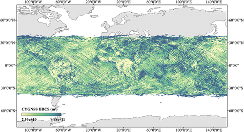
The CYGNSS constellation is composed of eight small satellites that were launched by the National Aeronautics and Space Administration (NASA) into a 580 km, 35° inclined equatorial orbit in December 2016. The CYGNSS mission provides quasiglobal coverage within ±38° in latitude (Figure 1) (C. C. Chew and Small 2018), with a median revisit period of only 3 hours (Ruf et al. 2016). Each satellite with a GNSS-R receiver is qualified to track and process four L-band GPS signals simultaneously. Considering this point, CYGNSS works as a multistatic radar (a system in which signals from multiple far-distance transmitters to the receiver can be detected simultaneously). In this way, 32 distinct observations of the Earth’s surface, forming the so-called delay Doppler map (DDM), can be obtained at a certain point in time based on all eight satellites. The applied CYGNSS data (Level 1 version 3.0), including DDMs, bistatic radar cross-sections (BRCSs) (Figure 1), and other geographic measurement information, can be obtained freely online (Jia et al. 2021). Data spanning the year 2018 and covering the entire region observed by CYGNSS were analyzed. The spatial resolution of this mission varies from 0.5 km to 25 km for specular (Fresnel zone size) and diffuse reflections (glistening zone size), respectively (Eroglu et al. 2019), which is a significant feature of CYGNSS data that is utilized in this study.

Figure 1. CYGNSS BRCSs of all eight satellites from 2018.1.1–2018.1.3.

The resolution of a single CYGNSS measurement is influenced by the incidence angle as well as the correlation between the diffuse scattering and specular reflection of the signal. The resolution changes with variations in the surface conditions and incidence angles. It is hypothesized that the signal received from the ground surface is mainly dominated by the coherent component, eventually reduced by roughness, and attenuated by vegetation. The CYGNSS BRCS σ can be used to obtain the reflectivity ${\mathrm{\Gamma }}_{\mathit{lr}}\left(\mathit{\theta }\right)$at a local incidence angle $\mathit{\theta }$, which has been demonstrated to be optimal for SM estimation (Eroglu et al. 2019):

(1) $\begin{array}{c}{\mathrm{\Gamma }}_{\mathit{lr}}\left(\mathit{\theta }\right)=\frac{\sigma {\left(R_t+R_r\right)}^2}{4\mathrm{\Pi }{\left(R_t{R}_r\right)}^2}\end{array}$(1)

where σ is the bistatic radar cross section in m² and the subscript lr denotes the left-hand circularly polarized (LHCP) downward-looking GNSS-R antenna. The symbols $R_t$ and $R_r$are the distances from the transmitter and receiver to the SP, respectively.

The reflectivity obtained after surface reflection is used to indicate changes in SM, but it is attenuated by vegetation and reduced by roughness. Here, attenuation by vegetation cover is adjusted based on land types (LTs), and the surface roughness is resolved based on the CYGNSS trailing edge slope (TES) in SM estimation (Eroglu et al. 2019; Jia et al. 2022; Senyurek et al. 2020b).

2.2. SMAP dataset

NASA launched the SMAP satellite in 2015, primarily for the purpose of monitoring SM and freeze – thaw cycles across the Earth using a radiometer (L-band) that penetrates up to 5 cm below the surface. The data and processed products are released through the official website and can be downloaded freely (Jia et al. 2021). In this study, the SMAP radiometer (Level 3) SM product, which provides SM data at resolutions of 9 km and 36 km in EASE grid form, was utilized. The land types (LTs) provided by the SMAP SM product were utilized as supplementary variables for both model training and prediction (Jia et al. 2022).

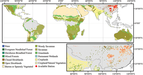
LTs refer to the different classifications or categories of land surfaces based on their characteristics and usage. The LT information was relatively stable and obtained from various data sources, making it more reliable than other ancillary data types that were adopted in previous studies (Eroglu et al. 2019). The IGBP (International Geosphere-Biosphere Programme) classifies land into 17 distinct types. An overview of the whole study area and the land classification process that is performed based on the most dominant LT with more than 50% coverage within each grid is provided in Figure 2.

Figure 2. Overview of the study area and IGBP LT provided by SMAP in 2018.

2.3. Independent in situ data

Independent validation was performed using ground-truth data obtained at China’s ground-based SM observation stations (Yan et al. 2022). The distribution of stations used in this study and their corresponding coverage areas are shown in Figure 2. Each observation station provides SM measurements at 10-cm intervals, starting from the soil surface and extending to a depth of 100 cm, on an hourly basis. Taking the penetration depth of the L-band into consideration, only topsoil moisture measurements (0 ~ 10 cm) were selected (Ma et al. 2023; Yan et al. 2022). The daily SM data also include geographic location information for each sampling site, such as latitude (La) and longitude (Lo).

2.4. Data quality control

The employed input data were filtered using several criteria as follows. (1) Only CYGNSS reflectivity values that were positive and below 0.1 were retained (Yan et al. 2022). (2) The data obtained at elevation angles smaller than 30° were excluded to effectively remove very weak signals (which may have resulted in the inclusion of noisy DDMs and errors in the SM estimations) from the sidelobe of the circular polarization antenna (Al-Khaldi et al. 2019; Yang, et al. 2020). (3) The antenna gain must be positive to ensure that only high-quality data obtained from left-hand circularly polarized (LHCP) signals are used (Yang, et al. 2020; C. Chew et al. 2016; Eroglu et al. 2019; Senyurek et al. 2020a). (4) Observations with DDM peak values in the range of 5 to 11 delay bins were retained from the dataset to avoid the inclusion of high-altitude measurements (Senyurek et al. 2020b; Rodriguez-Alvarez et al. 2019). (5) The SMAP “retrieval recommended” quality flag was used to filter the SMAP data (Senyurek et al. 2020a). Table 1 shows the total numbers of one-week CYGNSS samples remaining at the 36 km, 9 km, and 3 km resolutions after the application of several quality control steps.

Table 1. The numbers of one-week samples used for CYGNSS SM estimation corresponding to different land types (LTs).

Land type (IGBP)	CYGNSSS (3 km)	CYGNSSS (9 km)	CYGNSSS (36 km)
All LTs	647937	422364	89975
Evergreen Needleleaf Forest	55	33	5
Deciduous Broadleaf Forest	40	26	8
Mixed Forests	135	88	17
Closed Shrublands	963	644	132
Open Shrublands	180103	115465	22716
Woody Savannas	46619	31822	8187
Savannas	58132	40158	10394
Grasslands	70529	45642	8958
Permanent Wetlands	132	87	29
Croplands	76905	48625	9495
Cropland/Natural Vegetation Mosaic	21417	14795	4018
Barren or Sparsely Vegetated	188889	122307	26015

3. Theory and methods

3.1. Overall flowchart

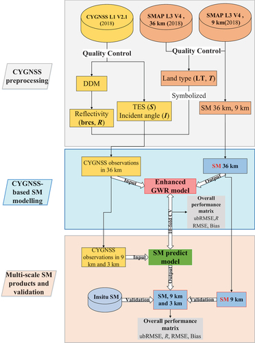
In this study, we introduce a novel approach for utilizing the GWR algorithm to derive a CYGNSS-based high-resolution SM product. The proposed framework includes three stages: a preprocessing stage, an SM modeling stage, and a validation stage (Figure 3).

Figure 3. The flowchart of the preprocessing, SM modeling, and validation stages of the proposed model.

3.1.1. Data preprocessing stage

The primary data sources utilized for estimating SM are the CYGNSS and SMAP datasets. These two datasets are preprocessed with a quality control procedure to extract the useful observations and reference SM.

3.1.2. SM modeling stage

In this stage, the objective is to establish an SM prediction model between the features extracted from the CYGNSS data and the reference SMAP SM without using other ancillary data. The enhanced GWR model is applied to establish the model relationship, which is effective for detecting the heterogeneity of spatial data and achieves high accuracy. The SM prediction model is built, and the overall performance matrix of different modeling methods is compared to that of SMAP SM using the 10-fold cross-validation (CV) method.

Cross-validation is a critical evaluation technique in ML and statistical modeling that aims to prevent overfitting and improve model generalization (Eroglu et al. 2019; Jia et al. 2021). In 10-fold cross-validation, the dataset is divided into 10 equal parts or “folds.” An iterative procedure is then conducted 10 times. The model is trained based on nine training folds and evaluated based on the remaining validation fold. This process is repeated for each distinct validation fold, ensuring that every example in the dataset is used for validation exactly once. The 10-fold CV process is commonly used to verify the accuracy and generalizability of models, including in cases with unseen data.

3.1.3. SM validation stage

After the SM modeling stage, the generated CYGNSS-based multiscale and SMAP SM products are obtained and validated. First, the input CYGNSS observations are gridded to 9 km and 3 km to apply the established SM prediction model. Then, the outputs of the 3 km and 9 km fine-scale SM products are compared with the SMAP 9 km and 36 km products for evaluation. Moreover, an additional validation process based on an independent data source, namely, data from an in situ SM network, is added. The outputs of the 9 km and 3 km fine-scale SM products are projected onto the same grid as the ground-truth SM data. If multiple sites are present in one grid, the average value of these sites represents the true observed value for that grid. The overall performance of this method is assessed based on several evaluation metrics.

3.2. Constructing an enhanced GWR algorithm with a variable data window

Remote sensing data often exhibit spatial heterogeneity, meaning that the data can vary significantly in space. A general linear regression model may not adequately capture complex spatial patterns and may not fully reflect the true characteristics of remote spatial data. In this study, the GWR model was adopted, as it is simple and effective and can learn local features as weighted references. Different spatial relationships and regression coefficients may be considered, thus enabling the description of the heterogeneity of spatial data. By establishing a local regression model for each point in the spatial range, it is possible to investigate the spatial variations and associated driving factors at a specific scale. The GWR calculation can be expressed as follows (Brunsdon Fotheringham and Charlton 1998; Fotheringham Brunsdon and Charlton 2002):

(2) $\begin{array}{c}{y}_i={\beta }_0\left(m_i,n_i\right)+\sum _{\mathit{j}=1}^k{\beta }_j\left(m_i,n_i\right)x_{\mathit{ij}}+{\epsilon }_i\end{array}$(2)

where $y_i$ is the dependent variable at the ith observation, $x_{\mathit{ij}}$ is the jth explanatory variable for each point $\mathit{i}\mathit{\hspace{0.17em}}(\mathrm{i}=$ 1, 2, … , k), and k is the number of available ancillary variables. The symbols $m_i\mathrm{and}{n}_i\mathit{\hspace{0.17em}}$are the projected spatial coordinates. The intercept value is denoted by ${\beta }_0\left(m_i,n_i\right)$, and ${\beta }_j\left(m_i,n_i\right)$ represents the regression coefficient, which reflects the effect of the jth explanatory variable $x_{\mathit{ij}}$ on dependent variable $y_i$. Additionally, ${\epsilon }_i$ is the error associated with the ith observation.

The symbol ${\beta }_j\left(m_i,n_i\right)$ can be evaluated using the local weighted least squares method, as shown in the following equation (Fotheringham, Brunsdon, and Charlton 2002; Huang Wu and Barrv 2010):

(3) $\begin{array}{c}\mathit{\beta }\left(m_i,n_i\right)={\left[X^T\mathit{W}\left(m_i,n_i\right)\mathit{X}\right]}^{-1}{X}^T\mathit{W}\left(m_i,n_i\right)\mathit{Y}\end{array}$(3)

Here, X is the matrix of explanatory variables, and Y is the dependent variable vector. $\mathrm{W}\left(m_i,n_i\right)=\mathit{diag}\left(w_{\mathit{i}1},w_{\mathit{i}2,}\dots ,w_{\mathit{in}}\right)$represents a spatial weight matrix, with the diagonal element $w_{\mathit{ij}}\left(1\le \mathit{j}\le \mathit{N}\right)$ indicating the weight assigned to point $\mathit{j}$ that is adjacent to point $\mathit{i}$, such that data points closer to point $\mathit{i}$ are assigned higher weights than those located farther away from point $\mathit{i}$ (Huang Wu and Barrv 2010). Popularly used weighting functions include the Gaussian, exponential, and tricube kernel functions (Chen et al. 2021).

The bandwidth determines which nearby observations are considered when calibrating coefficients for a local point. Changing the spatial kernel function or bandwidth may change the coefficient estimates (Cho et al. 2009). Most bandwidth is fixed, especially in cases with homogeneous and dense distributions of selected grids or standard geographic scales. Here, it should be noted that the optimal bandwidth (e.g. the optimal number of neighbors) for our study was determined through an adaptive statistical optimization process. Since the surface reflection points of CYGNSS are randomly distributed, multiple points may exist within a single grid. Therefore, using a fixed window size to select the training data is not suitable for CYGNSS estimation. To account for the optimal neighbor points, the size of the neighbor window (N) and the number of reflection points in one grid ($N_{\mathit{threshold}}$) can be calculated and optimized iteratively as follows:

(4) $\begin{array}{c}\mathit{N}=\mathit{M}\ast N_{\mathit{threshold}}\end{array}$(4)

The symbol $N_{\mathit{threshold}}$ is a critical factor that provides the numbers of points in the local grid that is first used in calculations for each prediction. The neighbor window size N should be at least larger than the local grid scale $N_{\mathit{threshold}}$ and can be optimized iteratively by adjusting the hyperparameter M (generally above 1). This procedure often includes trial-and-error iterations and uses a specific technique, such as a brute force search or a random search (optimized to 3 in this study). The goal is to find the optimal parameters that minimize the error or maximize the accuracy of the model.

In this case, fewer neighbor points are selected in areas where data points in one grid are sparse, and more neighbors are selected in areas where data points in one grid are dense. This strategy can greatly mitigate the tendency to only consider the reflection points within the local grid and neglect the features of the surrounding grids.

Notably, the optimal window size N is a variable that is adjusted based on the density of sample data in each regression grid. It refers to the process of continuously refining and improving a solution through repeated iterations. This strategy, called the “spatially adaptive window” technique, addresses the issue of unevenly distributed reflection points in CYGNSS data, resulting in significant time savings and contributing to self-adjusting CYGNSS SM estimation.

3.3. Generating CYGNSS-based multiscale SM products

Until now, high-resolution SM estimation with CYGNSS data has been limited to simple gridding or averaging, and the resolution is fixed during the estimation process. However, CYGNSS data are associated with reflectivity changes due to variations over land. In this investigation, the proposed multiscale scheme enables us to fully exploit the variable-spatial-resolution features of CYGNSS observations and simultaneously obtain multiscale high-resolution SM products.

The established functional relationship between CYGNSS observations and SM at a coarse resolution can be defined as follows:

(5) $\begin{array}{c}\mathit{S}{M}_{\mathit{smap},36\mathit{km}}=f_{\mathit{gwr}}{\left({\mathit{R}}_{\mathit{cygnss}},\mathit{TES},\mathit{LT}\right)}_{36\mathit{km}}\end{array}$(5)

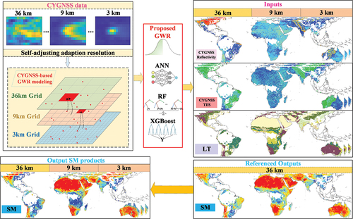
where $\mathit{S}{M}_{\mathit{smap},36\mathit{km}}$ is the reference SMAP SM at 36 km. $R_{\mathit{cygnss}},\mathit{TES},\mathrm{and}\mathit{LT}$ denote the CYGNSS reflectivity, CYGNSS trailing edge slope and LT based on SMAP data. The enhanced GWR model was applied to describe the spatially nonstationary relationships between variables. After the GWR-based SM prediction model was built, these functional relationships were preserved and transferred to obtain a high-resolution SM product (Figure 4). The self-adjusting adaptative resolution process for obtaining a downscaled SM product at a fine scale, such as 3 km CYGNSS observations, is expressed as follows:

Figure 4. Diagram of the generation of the proposed multiresolution SM product.

(6) $\begin{array}{c}\mathit{S}{M}_{\mathit{cygnss},\mathit{adaptive}}=f_{\mathit{gwr}}{\left({\mathit{R}}_{\mathit{cygnss}},\mathit{TES},\mathit{LT}\right)}_{\mathit{adaptive}}\end{array}$(6)

where $\mathit{S}{M}_{\mathit{cygnss},\mathit{adaptive}}$ is the estimated SM with a self-adaptive resolution. $R_{\mathit{cygnss}},\mathit{TES},\mathrm{and}\mathit{LT}$ denote the corresponding CYGNSS reflectivity, CYGNSS trailing edge slope and LT based on SMAP data, respectively.

The diagram of the proposed approach applied to generate the multiscale SM product (Figure 4) is presented. First, we established a model between key SM and CYGNSS observations at a coarse resolution (36 km). The model was designed to simulate the relationship between the CYGNSS parameters and SM and was subsequently applied at a fine scale to predict the corresponding SM. The CYGNSS data provide users with the opportunity to freely set the desired resolution for the grids of SM products as needed (e.g. 36 km, 9 km or 3 km). A fine resolution of 3 km was adopted to investigate the capability of using CYGNSS observations to produce high-resolution SM products since most 3 km grid cells have only one CYGNSS reflection point and thus may represent the highest resolution of the CYGNSS system. Concurrently, the downscaled SM product was validated with an independent SM source (e.g. data from an in situ SM network).

As shown in detail (Figure 4), the proposed enhanced GWR model was built for each image coordinate in the SMAP and CYGNSS image sets (36 km spatial resolution). For each local GWR model, the SMAP and CYGNSS EASE grids for data from adjacent grid coordinates collected with an adaptive window were reserved as the observation pairs for the dependent and independent variables, respectively. The regression weight for each observation pair was then assigned according to the distance from the grid center coordinate of the selected grid pair to the center grid coordinate used in the current GWR model. A dedicated GWR model was created for each grid coordinate observed at the 36 km spatial resolution. Once the regression coefficients (36 km) were estimated, the predicted values (9 km or 3 km) were computed for each location in space by substituting the nearest local estimates of the regression coefficients (36 km) into the regression equation. It was assumed that the regression coefficients for the grid cells at 36 kilometers and the closest 9 kilometers were the same.

The input explanatory variables were CYGNSS reflectivity, CYGNSS TES, and LT. The output of the model was the referenced SMAP SM. The regression equation in GWR was calibrated using known explanatory variables and dependent variables, and new output estimates were obtained from fine-scale explanatory variables. The regression coefficients were saved, and coarse CYGNSS images were replaced with the corresponding fine-scale images to train the model and acquire fine-scale SM estimates.

Overall, the unique feature of the variable resolution of CYGNSS data was exploited to create a fine-resolution SM, and this approach is “self-adaptive” for modifying the SM scale as needed. Unlike traditional downscaling SM estimation, few parameters are needed in this approach. There is no external data source and only one ancillary source from SMAP. It circumvents the need for external high-resolution auxiliary data, which helps achieve multiscale CYGNSS-based SM estimation and supports a wealth of possibilities for implementing independent estimation based on CYGNSS satellites.

4. Results and analysis

4.1. Feature optimization

The input variables include reflectivity (R) derived from BRCS, TES (S) calculated from DDM, the incidence angle (I), and LT labels (T). To find the optimal subset of features that maximizes the performance of the model, the selection of input variable combinations was first analyzed by comparing the results of three variants: (1) R+I+S, (2) R+T+S, and (3) R+T+I+S. Table 2 reports the results of SM feature optimization tests based on global CYGNSS 36 km data over three days.

Table 2. Feature optimization comparison (tricube kernel) for CYGNSS SM estimation at 36 km (three days).

GWR	Variant	ubRMSE(cm^3/cm^3)	R	RMSE(cm^3/cm^3)	abs (Bias) (cm^3/cm^3)
All types	R+T+I+S	0.0298	0.9423	0.0298	0.0002
	R+T+S	0.0301	0.9413	0.0301	0.0001
	R+I+S	0.0300	0.9416	0.0300	0.0002

As mentioned before, an enhanced GWR model with a spatially adaptive window was adopted. The key variable window $\mathit{N}\mathit{\hspace{0.17em}}$was tested and optimized (M = 3). We observed that all the variants exhibited good performance in terms of the statistical metrics. The R+T+I+S combination exhibited superior performance in terms of both the ubRMSE and correlation coefficient compared to the other variants. These results confirmed that these variables all play positive roles in our model. Notably, for the deciduous broadleaf forest and mixed forestland types, setting the appropriate incident angle can reduce the occurrence of scattering phenomena. Hence, the R+S+I+T variant was selected as the optimal variant for the following analyses.

4.2. Comparison with other advanced methods considering spatial location

In this study, we assessed the effectiveness of our suggested approach (advanced GWR) by comparing it with three other competing methods: the random forest (RF) algorithm, XGBoost, and an artificial neural network (ANN). These methods have demonstrated promising results in CYGNSS SM estimation (Eroglu et al. 2019; Jia et al. 2022; Senyurek et al. 2020b). To achieve a fair comparison with the proposed GWR model, which accounts for spatial variations in the relationships between variables, the ML and neural network models were applied with the same settings as the GWR model, including using latitude (La) and longitude (Lo) as the explanatory variables. Table 3 reports the SM estimation accuracy of all competing models. Among these models, the advanced GWR model performed best, followed by RF and XGBoost. The SM estimation results were obtained using all competing methods based on 10-fold cross-validation (CV), and the results are reported for different LTs (Table 3).

Table 3. SM estimation accuracy comparison of different methods considering spatial location at 36 km (one year).

LT	Methods (R+S+I+T, La+Lo)	ubRMSE (cm^3/cm^3)	abs(R)	RMSE (cm^3/cm^3)	abs (Bias) (cm^3/cm^3)
All types	GWR	0.0329	0.9311	0.0329	0.0003
	RF	0.0413	0.8879	0.0414	0.0011
	XGBoost	0.0428	0.8792	0.0428	0.0005
	ANN	0.0635	0.7095	0.0635	0.0006
Evergreen Needleleaf Forest	GWR	0.0481	0.4974	0.0491	0.0100
	RF	0.0399	0.9169	0.0399	0.0013
	XGBoost	0.0405	0.9141	0.0407	0.0035
	ANN	0.0596	0.8025	0.0596	0.0009
Deciduous Broadleaf Forest	GWR	0.2038	0.5272	0.2103	0.0516
	RF	0.0395	0.8808	0.0395	0.0007
	XGBoost	0.0423	0.8627	0.0423	0.0011
	ANN	0.0596	0.7036	0.0600	0.0065
Mixed Forests	GWR	0.0448	0.7898	0.0465	0.0127
	RF	0.0442	0.8909	0.0444	0.0036
	XGBoost	0.0517	0.8473	0.0518	0.0030
	ANN	0.0699	0.6951	0.0708	0.0113
Closed Shrublands	GWR	0.0239	0.9088	0.0246	0.0060
	RF	0.0405	0.8883	0.0405	0.0005
	XGBoost	0.0411	0.8840	0.0411	0.0006
	ANN	0.0607	0.7253	0.0607	0.0016
Open Shrublands	GWR	0.0244	0.8766	0.0244	0.0001
	RF	0.0411	0.8902	0.0411	0.0008
	XGBoost	0.0426	0.8811	0.0426	0.0003
	ANN	0.0639	0.7086	0.0639	0.0002
Woody Savannas	GWR	0.0449	0.8816	0.0449	0.0017
	RF	0.0417	0.8855	0.0417	0.0008
	XGBoost	0.0430	0.8772	0.0430	0.0003
	ANN	0.0635	0.7095	0.0635	0.0008
Savannas	GWR	0.0390	0.9003	0.0390	0.0007
	RF	0.0414	0.8864	0.0415	0.0010
	XGBoost	0.0429	0.8772	0.0429	0.0004
	ANN	0.0637	0.7056	0.0637	0.0009
Grasslands	GWR	0.0357	0.9289	0.0357	0.0005
	RF	0.0412	0.8900	0.0412	0.0009
	XGBoost	0.0427	0.8811	0.0427	0.0003
	ANN	0.0640	0.7083	0.0640	0.0000
Permanent Wetlands	GWR	0.1020	0.4992	0.1083	0.0365
	RF	0.0438	0.8980	0.0439	0.0040
	XGBoost	0.0448	0.8935	0.0452	0.0059
	ANN	0.0771	0.6266	0.0783	0.0140
Croplands	GWR	0.0428	0.9013	0.0428	0.0017
	RF	0.0411	0.8897	0.0411	0.0014
	XGBoost	0.0425	0.8810	0.0425	0.0008
	ANN	0.0629	0.7154	0.0629	0.0007
Cropland/Natural Vegetation Mosaic	GWR	0.0656	0.8130	0.0656	0.0010
	RF	0.0415	0.8848	0.0416	0.0015
	XGBoost	0.0429	0.8764	0.0429	0.0009
	ANN	0.0635	0.7059	0.0636	0.0019
Barren or Sparsely Vegetated	GWR	0.0185	0.8889	0.0185	0.0000
	RF	0.0416	0.8861	0.0416	0.0012
	XGBoost	0.0429	0.8779	0.0429	0.0006
	ANN	0.0633	0.7106	0.0633	0.0008

Different methods display slightly different behaviors for each LT, which is consistent with the finding that using different methods for each LT can aid in verifying the overall prediction results. Moreover, we observe that GWR achieves the lowest ubRMSE and highest correlation coefficient (R = 0.93) for most LTs compared with the other methods. For illustration, the density plots (3 days) displaying the SM estimation performance are presented in Figure 5. The clear consistency and generalizability between the reference and estimated SM products indicate the effectiveness of the proposed GWR model.

Figure 5. Density plot of SM estimations using different methods considering spatial location: (a) Proposed advanced GWR method, (b) RF, (c) XGBoost, and (d) ANN.

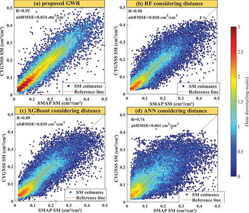
Normally, SM is highly related to the location of an observation point, that is, its longitude and latitude. GWR provides the possibility to incorporate these considerations into the model and can be used to calculate spatially varying relationships when predicting SM values, which could efficiently improve its accuracy. This could be the reason why compared to the other models, GWR yields a pronounced improvement in the results.

4.3. Evaluation of the proposed GWR-Based SM estimation of CYGNSS

After the feature selection and method comparison stages, the proposed GWR-based CYGNSS SM model with several weighting functions, namely, Gaussian, exponential, and tricube kernel functions, is investigated, and the results are reported in Table 4.

Table 4. GWR-based SM estimation accuracy with different weighting functions at 36 km (one year).

LT	Methods, GWR (R+S+I+T)	ubRMSE (cm^3/cm^3)	abs(R)	RMSE (cm^3/cm^3)	abs(Bias) (cm^3/cm^3)
All types	Tricube	0.0329	0.9311	0.0329	0.0003
	Exponential	0.0563	0.8220	0.0563	0.0003
	Gaussian	0.0627	0.7913	0.0627	0.0003
Evergreen Needleleaf Forest	Tricube	0.0481	0.4974	0.0491	0.0100
	Exponential	0.0369	0.5882	0.0408	0.0175
	Gaussian	0.0347	0.5864	0.0465	0.0310
Deciduous Broadleaf Forest	Tricube	0.2038	0.5272	0.2103	0.0516
	Exponential	0.2052	0.5212	0.2108	0.0481
	Gaussian	0.2052	0.5155	0.2109	0.0487
Mixed Forests	Tricube	0.0448	0.7898	0.0465	0.0127
	Exponential	0.0828	0.5846	0.0842	0.0157
	Gaussian	0.0748	0.6184	0.0763	0.0149
Closed Shrublands	Tricube	0.0239	0.9088	0.0246	0.0060
	Exponential	0.0223	0.9201	0.0246	0.0103
	Gaussian	0.0235	0.9106	0.0259	0.0108
Open Shrublands	Tricube	0.0244	0.8766	0.0244	0.0001
	Exponential	0.0238	0.8805	0.0238	0.0003
	Gaussian	0.0244	0.8737	0.0244	0.0003
Woody Savannas	Tricube	0.0449	0.8816	0.0449	0.0017
	Exponential	0.0669	0.7746	0.0669	0.0018
	Gaussian	0.0657	0.7827	0.0657	0.0018
Savannas	Tricube	0.0390	0.9003	0.0390	0.0007
	Exponential	0.0481	0.8532	0.0481	0.0003
	Gaussian	0.0840	0.6782	0.0840	0.0006
Grasslands	Tricube	0.0357	0.9289	0.0357	0.0005
	Exponential	0.0376	0.9204	0.0376	0.0009
	Gaussian	0.0381	0.9181	0.0381	0.0007
Permanent Wetlands	Tricube	0.1020	0.4992	0.1083	0.0365
	Exponential	0.1272	0.4724	0.1314	0.0329
	Gaussian	0.1310	0.4545	0.1341	0.0288
Croplands	Tricube	0.0428	0.9013	0.0428	0.0017
	Exponential	0.0454	0.8880	0.0454	0.0017
	Gaussian	0.0459	0.8855	0.0460	0.0015
Cropland/Natural Vegetation Mosaic	Tricube	0.0656	0.8130	0.0656	0.0010
	Exponential	0.2198	0.3756	0.2198	0.0034
	Gaussian	0.2361	0.3580	0.2361	0.0026
Barren or Sparsely Vegetated	Tricube	0.0185	0.8889	0.0185	0.0000
	Exponential	0.0184	0.8886	0.0184	0.0001
	Gaussian	0.0181	0.8923	0.0181	0.0000

The tricube function (R = 0.93) performs significantly better than the other two competing kernel functions. The exponential (ubRMSE = 0.0369 cm³/cm³) and Gaussian kernels (ubRMSE = 0.0347 cm³/cm³) are effective for LTs that rarely appear in small datasets (one week), such as evergreen needleleaf forests. Different functions display different performance levels for the same LT. Nevertheless, the tricube band was chosen as the optimal kernel band in this case. One should note that the tricube function displays stable performance even when the dataset is relatively small.

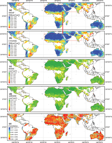
To investigate the estimation performance in terms of the obtained SM distribution, the SM values for each cell from SMAP and the GWR-based SM predictions were plotted, as shown in Figure 6. The values of RMSE, ubRMSE, and correlation distributions between the SMAP and CYGNSS-based estimates are also shown. The SM values based on CYGNSS agree with the reference SMAP SM. The findings reveal that the suggested GWR-based approach yields a mean ubRMSE of 0.0253 cm³/cm³, a mean RMSE of 0.0291 cm³/cm³. The color legend was generated using a natural breaks model. The SM estimates are highly correlated with the SMAP SM, with a mean R of 0.843. Since the estimation result of GWR is based on the calculations at surrounding points, one of the features of these results is that the predicted SM values tend to display an obvious patch structure, as indicated by the red box in Figure 6(a,b); that is, in a small region, the SM value changes little, which is consistent with the “First Law of Geography:” everything is related to everything else, but closer things are more related to each other (Tobler 1970). It also shows that in most regions, high SM values correspond to high values of both the RMSE and ubRMSE, which is consistent with previous studies (Clarizia et al. 2019; Jia et al. 2022). Additionally, the ubRMSE indicates improved performance compared to the RMSE since the ubRMSE is an unbiased version of the RMSE, as shown in Figure 6(d). The ubRMSE removes any systematic bias that may be present in the prediction or model, allowing for a fairer comparison of different models or prediction methods.

Figure 6. Annual mean values obtained with the natural breaks model (36 km): (a) SMAP SM, (b) GWR-based CYGNSS-predicted SM, (c) RMSE, (d) ubRMSE and (e) Correlation metrics.

4.4. Multiresolution GWR-based SM products of CYGNSS

In the previous sections, the GWR-based SM estimation method and the performance comparison analysis were described in detail at a large scale (36 km). In this section, the multi-scale SM products (9 km and 3 km) obtained with the proposed GWR-based approach are explored. Additionally, a comparison of accuracy and spatial distributions is performed.

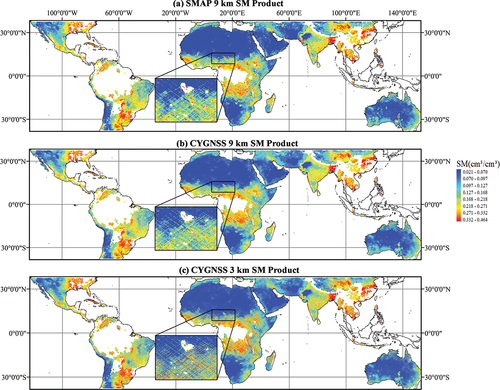
To visualize a complete multi-scale SM spatial distribution at the global scale, the one-year downscaled SM results were averaged to obtain the daily spatial distribution of SM (Figure 7). Figure 7(a) shows the SM distributions of the SMAP product at 9 km ($\mathit{S}{M}_{\mathit{smap}9}$), the downscaled GWR-based CYGNSS SM product at 9 km ($\mathit{S}{M}_{\mathit{gwr}9}$), and the downscaled GWR-based CYGNSS SM product at 3 km ($\mathit{S}{M}_{\mathit{gwr}3}$). The spatial distribution patterns of the downscaled SM products (9 km and 3 km) are similar to those of the SMAP product and CYGNSS SM at 36 km, as indicated by a comparison of Figures 7(b,c) and 6(a,b). In more densely vegetated areas, the SM content is relatively high, and the prediction accuracy is poor. This pattern is consistent with the phenomenon observed previously (Clarizia et al. 2019), which may be caused by an increase in noncoherent components due to the presence of dense vegetation. The outcomes reveal that the proposed scheme effectively transforms the spatial resolution of the CYGNSS-based SM product from 36 km to 3 km while maintaining the spatial distribution of SM, thus conforming to that of the SMAP SM data (e.g. $\mathit{S}{M}_{\mathit{smap}9}$).

Figure 7. Annual mean values of multiscale SM products: (a) SMAP SM 9 km, (b) Downscaled CYGNSS 9 km SM product, and (c) Downscaled CYGNSS 3 km SM product.

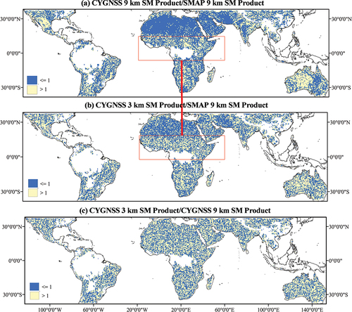
Additionally, the estimation errors were evaluated and are shown in Figure 8 as the ratio of the ratio of $\mathit{S}{M}_{\mathit{gwr}9}$ to $\mathit{S}{M}_{\mathit{smap}9}$, $\mathit{S}{M}_{\mathit{gwr}3}$ to $\mathit{S}{M}_{\mathit{smap}9}$, and the ratio of $\mathit{S}{M}_{\mathit{gwr}3}$ to $\mathit{S}{M}_{\mathit{gwr}9}$. To further analyze the error distribution, the ratio values were split into two cases: below and above one. Notably, the errors in the “above one” case are higher than those in the “below one” case. As indicated by the error ratio diagrams (Figure 8) of the multiresolution SM products, the 9 km and 3 km SM products agree well in most regions with the SMAP 9 km product, and the regions with large errors are mainly in central Africa and other regions with abundant vegetation. This phenomenon once again reveals that surface vegetation is the major error source for SM estimation based on CYGNSS. Notably, the error ratio diagrams of the two downscaled products (9 km/3 km) indicate that the error distribution is relatively uniform, which indicates that the proposed method provides good generalizability in terms of prediction performance in different regions, thus providing a new solution for future high-resolution SM estimation.

Figure 8. Annual mean values of error ratio diagram: (a) The ratio of $\mathit{S}{M}_{\mathit{gwr}9}$ to $\mathit{S}{M}_{\mathit{smap}9}$, (b)The ratio of $\mathit{S}{M}_{\mathit{gwr}3}$ to $\mathit{S}{M}_{\mathit{smap}9}$, and (c) The ratio of $\mathit{S}{M}_{\mathit{gwr}3}$ to$\mathit{S}{M}_{\mathit{gwr}9}.$.

To further illustrate the SM estimation performance of the CYGNSS-based SM products with the reference SMAP data. The mean values of the error matrix for comparing different satellite-based SMs at different resolutions are displayed in Table 5. As mentioned before, for the convenience of demonstration, $\mathit{S}{M}_{\mathit{smap}9}$ and $\mathit{S}{M}_{\mathit{smap}36}$ refer to the SMAP SM at 9 km and 36 km, respectively.

Table 5. Mean indicator spatial evaluation for multiresolution products compared to SMAP 36 km and 9 km SM during annual cycles.

Mean (cm^3/cm^3)	$\mathit{S}{\mathit{M}}_{\mathit{gwr}\mathit{9}}$ vs. $\mathit{S}{\mathit{M}}_{\mathit{smap}36}$	$\mathit{S}{\mathit{M}}_{\mathit{gwr}3}$ vs.$\mathit{S}{\mathit{M}}_{\mathit{smap}36}$	$\mathit{S}{\mathit{M}}_{\mathit{gwr}9}\mathit{\hspace{0.17em}}$vs.$\mathit{S}{\mathit{M}}_{\mathit{smap}9}$	$\mathit{S}{\mathit{M}}_{\mathit{gwr}3}\mathit{\hspace{0.17em}}$vs.$\mathit{S}{\mathit{M}}_{\mathit{smap}9}$
R	0.9536	0.9456	0.9435	0.9357
ubRMSE	0.026	0.0281	0.0288	0.0307
RMSE	0.026	0.0281	0.0290	0.0309
abs (Bias)	0.0001	0.0001	0.0038	0.0038

Both downscaled products, $\mathit{S}{M}_{\mathit{gwr}3}$ and $\mathit{S}{M}_{\mathit{gwr}9}$, exhibit excellent performance for all metrics. Notably, they exhibit a higher degree of similarity with $\mathit{S}{M}_{\mathit{smap}36}$ than with $\mathit{S}{M}_{\mathit{smap}9}$. Compared to $\mathit{S}{M}_{\mathit{gwr}3},\mathit{S}{M}_{\mathit{gwr}9}$ displays greater with $\mathit{S}{M}_{\mathit{smap}36}$. However, this advantage is less pronounced in the comparisons based on $\mathit{S}{M}_{\mathit{smap}9}$. The difference could be attributable to the distinct spatial patterns of the SMAP 9 km and 36 km products since the SMAP 36 km product was adopted to build the SM estimation model, while the SMAP 9 km product was used only for validation purposes. Therefore, comparisons of these two downscaled products ($\mathit{S}{M}_{\mathit{gwr}3}$ and $\mathit{S}{M}_{\mathit{gwr}9}$) with the $\mathit{S}{M}_{\mathit{smap}36}\mathit{\hspace{0.17em}}$product yield better results in terms of the relevant metrics than comparisons with $\mathit{S}{M}_{\mathit{smap}9}$. Nevertheless, both downscaled products exhibit good results, with mean R values above 0.9 and mean ubRMSE values of approximately 0.03 cm³/cm³. This also further shows that the multiresolution SM products retain the numerical information of the SM data well, thus demonstrating the numerical consistency of the SM downscaling method proposed in this paper.

4.5. Independent downscaling validation using in situ networks

In situ SM networks (Figure 9) were used to evaluate the performance of the proposed approach. First, we examined the overall performance of the observed and estimated SM during the entire period. In the evaluation process, when there was only one site within a grid, the in situ value was directly used as the true observed value of the grid for evaluation along with the satellite products. When there were multiple sites within a grid, the average value of the multiple sites was used as the true observed value of the grid. Table 6 shows the error metrics obtained based on the entire dataset from over 1000 sites.

Figure 9. Annually averaged SM at each ground site.

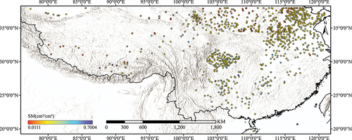
Table 6. The accuracy of the overall evaluation of the 3 km and 9 km SM products during annual cycles (over 1000 SM sites).

Overall (cm^3/cm^3)	$\mathit{S}{\mathit{M}}_{\mathit{gwr}3}$ vs. in situ	$\mathit{S}{\mathit{M}}_{\mathit{gwr}9}$ vs. in situ	$\mathit{S}{\mathit{M}}_{\mathit{smap}9}$ vs. in situ
R	0.8113	0.8201	0.8906
ubRMSE	0.0525	0.0503	0.0391
RMSE	0.0525	0.0503	0.0393
abs (Bias)	0.0004	0.0009	0.0034

Table 6 shows the values of each metric based on the entire dataset from approximately 1000 sites throughout the year. A performance comparison of the GWR-based SM products ($\mathit{S}{M}_{\mathit{gwr}9}$, $\mathit{S}{M}_{\mathit{gwr}3}$) and SMAP SM 9 km product ($\mathit{S}{M}_{\mathit{smap}9}$) with respect to the in situ values is shown. The ubRMSE of the CYGNSS-based product $\mathit{S}{M}_{\mathit{gwr}3}$ is 0.0525 cm³/cm³, which is slightly higher than the ubRMSE of the $\mathit{S}{M}_{\mathit{gwr}9}$ (0.0503 cm³/cm³).

Accordingly, using the correlation coefficient instead of the absolute error metrics may be more reasonable to evaluate the performance of satellite-based soil moisture products in such cases (Zeng et al. 2015). In most regions, the CYGNSS-based SM products ($\mathit{S}{M}_{\mathit{gwr}3}\mathit{\hspace{0.17em}}$ and $\mathit{S}{M}_{\mathit{gwr}9}$) are comparable to the $\mathit{S}{M}_{\mathit{smap}9}\mathit{\hspace{0.17em}}$product. Both CYGNSS-based products effectively capture the temporal variation in ground soil moisture, with a reasonable correlation coefficient above 0.8, demonstrating the effectiveness of capturing the SM dynamics with the CYGNSS data. The accuracy of the CYGNSS-based $\mathit{S}{M}_{\mathit{gwr}9}$ is slightly better than that for $\mathit{S}{M}_{\mathit{gwr}3}$, which agrees with the results in Table 5.

Moreover, to assess the contributions of different LTs, scatter plots with error statistics were added to show the deviation between in situ measurements and satellite-based products at 9 km, as illustrated in Figure 10. When the scatter points are above the 1:1 line, the SM is overestimated compared to the in situ data, and vice versa for scatter points below the 1:1 line. The SMAP and CYGNSS products are generally very close to the 1:1 line but exhibit different behaviors for various land surface types.

Figure 10. Scatter plots for accuracy evaluations of different land types at the annual scale: (a) All samples, (b) Mixed forests, (c) Open Shrublands, (d) Woody Savannas, (e) Grasslands, (f) Croplands, (g) Cropland/Natural vegetation mosaic and (h) barren or sparsely Vegetated.

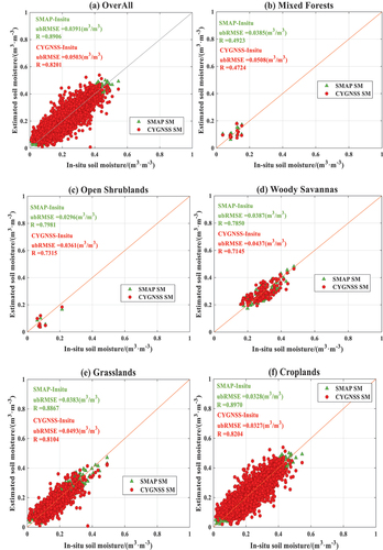
Figure 10. (Continued).

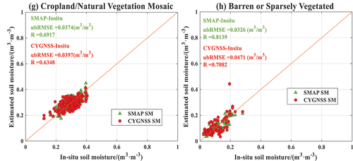
For most LT classifications, the CYGNSS and SMAP products display similar performance. However, for the classification of mixed forests, CYGNSS displays poorer performance, with a higher ubRMSE of 0.0508 cm³/cm³, which is approximately 0.03 higher than that of SMAP. For the classification of croplands, CYGNSS SM estimates are slightly better than the SMAP product values, with an unRMSE of 0.0327 cm³/cm³. The reason for the former phenomenon in mixed forests is likely due to unstable GPS signal reception, which may be caused by the obstruction and scattering of signals by dense trees and vegetation. The latter phenomenon in croplands could be attributed to CYGNSS having a higher temporal resolution, allowing for land use change due to cultivation activities to be accurately and quickly captured, thus resulting in more accurate SM values.

To illustrate this phenomenon more clearly, the number of estimated points below the 1:1 line and the proportion of such points with respect to the total number of points were determined. In Table 7, the percentages of CYGNSS points below the 1:1 line corresponding to different LTs were 0.30, 0.71, 0.57, 0.63, 0.58, 0.57 and 0.47. For SMAP data, these values were 0.53, 0.71, 0.50, 0.60, 0.57, 0.57 and 0.40. The CYGNSS and SMAP products exhibit similar behaviors, with general underestimation of SM for most LTs. However, for the classification of mixed forest, the CYGNSS approach overestimates SM (30.77%), but SMAP underestimates SM (50.85%). The deviation of the CYGNSS-based estimates is larger than that for the SMAP data. This phenomenon can be explained by the fact that dense trees lead to more diffuse scattering and weaken the signal reception of CYGNSS reflectivity (Jia et al. 2022), as mentioned before. The findings demonstrate that the estimation accuracy of the CYGNSS SM product differs from that of the SMAP product due to differences in land surface characteristics, thus providing theoretical support for future hybrid applications and the development of both SM products.

Table 7. Statistics for the points located below the 1:1 line in the scatter plot.

Type		CYGNSS			SMAP
	Number of points	Above the 1:1 line	Below the 1:1 line	Below-line percentage (%)	Above the 1:1 line	Below the 1:1 line	Below-line percentage (%)
All types	5333	2188	3145	58.97%	2263	3070	57.57%
Mixed Forests	13	9	4	30.77%	6	7	53.85%
Open Shrublands	7	2	5	71.43%	2	5	71.43%
Woody Savannas	141	60	81	57.45%	70	71	50.35%
Grasslands	771	281	490	63.55%	301	470	60.96%
Croplands	4095	1697	2398	58.56%	1737	2358	57.58%
Cropland/Natural Vegetation Mosaic	214	91	123	57.48%	92	122	57.01%
Barren or Sparsely Vegetated	92	48	44	47.83%	55	37	40.22%

Additionally, due to differences in both spatial resolution and vertical resolution between satellite and in situ data, it makes more sense to compare time series trends than specific values (Owe de Jeu and Holmes 2008). A detailed time series comparison conducted during this study is presented in Figure 11, which shows the temporal variations in SM estimated based on CYGNSS data, the SMAP product, and the in situ average SM from January 1 to 31 December 2008. The average SM measurements at all sites were compared with the SM products, which were also averaged over all grids. The same technique has been used in many previous studies for validation purposes (Jackson et al. 2010, 2012; Leroux et al. 2014; Su de Rosnay et al. 2013; Su et al. 2011).

Figure 11. Temporal variation comparisons of the station-averaged SM estimates and satellite SM products: SM estimated by the proposed CYGNSS-based algorithm and SMAP SM product with in situ SM at Chinese network sites.

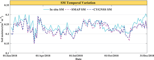
Generally, all SM data fit well with in situ SM to a certain degree. The overall trend of the temporal dynamics of SM can be well captured by the SMAP and CYGNSS datasets. However, the SMAP SM and CYGNSS SM exhibit significant deviations (underestimation or overestimation) in some periods, such as March to April and September. Specifically, the temporal variation results obtained using the proposed algorithm display a good fit to the in situ data, with R = 0.74. The satellite SM products appear to underestimate SM throughout the period. This conclusion is consistent with that of Zhao et al. (2011b), who also found that the NASA-derived SM levels were obviously lower than the actual SM levels. As a result, the overall evaluation results not only validate the capability and performance of the proposed method but also verify that the CYGNSS-based downscaled SM is an excellent complement to the SMAP product in terms of its high spatial resolution.

5. Discussion

5.1. Possible uncertainties related to the modeling data

The possible uncertainties for CYGNSS-based SM estimation are associated with several factors. The first is the uncertainty of the datasets. The estimation of SM from GNSS-R data is an intrinsically ill-posed problem since the behavior of the reflected signal depends on many other parameters in addition to SM. In particular, soil roughness, in addition spectral scattering, scatters the electromagnetic energy in many directions, and vegetation attenuates the direct signal and further contributes to signal diffusion. The CYGNSS reflectivity has a high weight among the variables used in the prediction, and this weight is positive, as an increase in SM increases the soil permittivity and thus the Fresnel coefficient (Clarizia et al. 2019). Roughness and vegetation are associated with smaller weights, as expected, but the compensation of them can still produce contribute to improvements in SM estimation performance.

Ancillary data are needed in the current stage since complete independent SM estimation relying solely on CYGNSS data has not been realized. In state-of-the-art studies, ancillary data from several different data sources are generally used. Table 8 provides a summary of several typical schemes for high-spatial resolution CYGNSS SM estimation. These large ancillary feature sets can increase costs and cross-correlated features, potentially resulting in marginal or reduced performance. Additionally, uncertainties and internal errors may be present in the ancillary data from different sources. Hence, minimizing the number of ancillary features while ensuring accuracy is one of the concerns of CYGNSS-based SM estimation. In this study, there is no external data source and only one ancillary feature (LT) from the SMAP product. The SMAP LT may contain some uncertainties caused by the complicated physical retrieval process. In addition, the accuracy of the SM ground-truth station measurements can influence SM estimation.

Table 8. Typical retrieval schemes and performance for high-resolution CYGNSS SM estimation.

Source	Scale	SM for validation	Num. of ancillary records	Adopted algorithms	Overall performance	Spatial resolutions
Kim and Venkat (2018)	Regional	SMAP	1	regression	R = 0.68–0.77	9 × 9 (km)
Eroglu et al. (2019)	Regional	In situ (ISMN)	5	ANN	ubRMSE=0.054 cm^3/cm^3, R=0.90	9 × 9 (km)
Senyurek et al. (2020a)	Regional	In situ (ISMN)	5–7	RF/ANN/SVM	RMSE=0.052/0.061/0.065 (cm^3/cm^3), R = 0.64–0.89 (RF)	9 × 9 (km)
Senyurek et al. (2020b)	Global	In situ (ISMN)	5–7	RF	mean ubRMSD=0.044 cm^3/cm^3, RMSD=0.066 cm^3/cm^3, R = 0.66	9 × 9 (km)
Yan et al. (2022)	Regional	In situ networks	1	Regression tree	RMSE=0.05 cm^3/cm^3, R = 0. 86	7 × 7 (km)
Tang and Yan (2022)	Regional	In situ networks	6	SVR	R = 0.87	10 × 10 (km)
Lei et al. (2022)	Global	SMAP and in situ networks	3	Random forest	ubRMSE=0.0543 cm^3/cm^3, R=0.4–0.8 (vs. in situ)	9 × 9 (km)
Nabi et al. (2022)	Regional	SMAP and in situ networks	8	CNNs	mean ubRMSE=0.0366 cm^3/cm^3, R=0.93 (vs. SMAP)	9 × 9 (km)
Proposed method	Global	SMAP and in situ networks	1	GWR	mean RMSE=0.0291 cm3/cm3, ubRMSE = 0.0329 cm3/cm3, R = 0.93 (vs. SMAP) ubRMSE = 0.0525 cm3/cm3, R = 0.81(vs. in situ)	3 ×3 (km)

The second is the concern about the phenology of vegetation. The phenology of vegetation refers to the study and observation of the timing and seasonal patterns of plant life cycle events, such as leaf emergence, flowering, fruiting, and senescence. Considering the phenological stage of vegetation is crucial for accurately analyzing sensor signals and effectively interpreting remote sensing data for different applications. Variations in phenological stages across different plant species or ecosystems can lead to differences in the timing and magnitude of changes observed in sensor signals. To mitigate the uncertainty from the phenology of vegetation, one-year data covering all four seasons from spring to winter were employed to build and test the SM estimation model. The results indicated that the model performed well within a one-year time range. The good performance may be attributed to the strong penetration capabilities of the L-band signals employed by CYGNSS satellites. This is also one of the advantages of GNSS-R remote sensing technology.

The findings presented previously suggested that remotely sensed SM products can effectively reflect the seasonal variations in ground SM, but some of them do not consistently meet the expected precision requirements. The deviation between the satellite-based and in situ SM might originate from discrepancies in spatial observation scales, as values associated with in situ data points and satellite pixels are compared. Moreover, bias may be caused by the inconsistencies between the depth of in situ SM measurements and the penetration depth of microwaves. The penetration depth of the electromagnetic wave in soils can vary from several centimeters (Li et al. 2018; Yan et al. 2022), depending on the SM level and soil type (e.g. approximately 0–5 cm for the L band and 0–10 cm for in situ topsoil adopted in this study). The soil depth inconsistency also partially contributes to some uncertainties in our results (Ma et al. 2023; Zeng et al. 2015; 2016).

Several factors that contribute to uncertainty were considered in this study. First, a temporal evaluation was carried out to reduce the inherent uncertainties in the scale differences between in situ points and satellite pixels (Ma et al. 2019). Due to the lack of ground SM observations that accurately represent the same scale as that of the satellite observations, we utilized the average point-based measurements as the “ground truth” (Zeng et al. 2015). Second, some studies have noted that the correlation coefficient and ubRMSE are less sensitive to spatial mismatch than RMSE or bias and thus (Zeng et al. 2015). Thus, this article has strengthened the analysis of R and ubRMSE, and weakened the evaluation of bias and RMSE. Moreover, we focus more on developing effective algorithms and mitigating the possible errors of the parameters in the SM algorithms (Zeng et al. 2016), potentially contributing to further improvements in the current CYGNSS-based estimation methods.

5.2. Effect of the amount of data in the GWR model

In this paper, an enhanced GWR-based model is proposed to estimate fine-resolution SM by considering nonlinearity and spatial heterogeneities. Compared with the traditional ML and neural network models, which also consider spatial distance, the location-space-specific GWR model yields better results. Two essential issues need to be addressed.

One is the number of samples, and the other is the computational cost. For the first issue, it should be noted that the CYGNSS reflection points are randomly distributed, which means that there may be multiple CYGNSS observations that fall into one grid, while no observations are in a neighboring grid. The CYGNSS observations and SMAP SM from 1 day and 3 days are shown in Figure 12. SMAP can provide intensive spatial global coverage over a three-day period. In typical cases, the average value of the SM reference from SMAP over a three-day period is commonly used as the daily reference for CYGNSS explanatory features. They are ideally treated as daily representatives by neglecting data variations within the three-day interval.

Figure 12. Comparison of data coverage: (a) SMAP 1-day SM, (b) SMAP 3-day SM, (c) CYGNSS 1-day BRCS, and (d) CYGNSS 3-day BRCS.

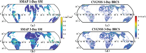
To establish a precise model, it is common to utilize data spanning at least an entire year while simultaneously accounting for the impact of phenology. Global modeling methods such as ML or ordinary linear regression assume a uniform relationship between explanatory variables and the dependent variable across the entire dataset. Long time series data can be directly applied as matrixes by ignoring the time stamp attributes. Actually, this operation is not problematic since a large sample size generally improves model learning performance, reduces overfitting, and enhances stability when establishing ML and neural network models.

GWR supports a more fine-scale spatial analysis by considering spatial heterogeneity and location effects. The local regression coefficients are considered at each individual point based on the data at neighboring points. In this case, the long time series data cannot be regarded as a matrix without considering the time stamp. Local regression was performed to identify which point is the closest to the estimation point on the same day. Hence, the CYGNSS panel data were separated into individual time units (3-day data) to perform modeling to greatly avoid null grids in this work. The GWR model, which was specifically designed for regression problems, is inherently effective in cases with relatively limited samples. Moreover, if long-time-series CYGNSS-based SM estimation is needed, GTWR (geographically and temporally weighted regression), as an extension of GWR that incorporates both spatial and temporal heterogeneity, can be applied.

Notably, to obtain a fair comparison with the GWR model, the ML and neural network models were applied with the same settings as those in GWR, including using the distance as the explanatory variable. The estimation performance of the ML and neural network models was improved by considering the distance factor. In future work, long-time-series CYGNSS data may be applied to the GTWR model and compared with the results of ML algorithms by considering both temporal and spatial effects.

For the second issue, as the GWR model was applied at every location, the computational cost was notably higher that of the global ML and neural network models. This challenge was addressed in two aspects in our work. On the one hand, the samples with weights that were below a certain threshold were excluded in the establishment of the GWR model. On the other hand, as mentioned before, long-time-series CYGNSS data were separated into modeling units, and the designed spatially adaptive window was applied to accommodate the CYGNSS data volume.

5.3. Role of the GWR-based model in the framework

The proposed GWR model was compared with popular ML and neural network-based CYGNSS SM estimation models, e.g. XGBoost, RF, and ANN (Eroglu et al. 2019). Moreover, the downscaling framework was used to integrate CYGNSS data and multiple biogeophysical factors (e.g. land cover and TES) to downscale SM. The GWR model estimates the local optimal spatial weights with an adaptive statistical optimization process and quantifies the spatial distribution of local regression coefficients, yielding fine-resolution SM estimates at different scales. The regression coefficients vary spatially with the land cover and terrain. Despite this spatial variability, the spatial patterns of SM can be adequately modeled with the GWR approach.

Emerging AI methods such as ML and advanced neural approaches are strong data-driven tools for data analysis, mining, and forecasting (Xu et al. 2021). AI models have become very popular in recent years, with considerable theoretical and technical progress in CYGNSS-based fields. A key issue in ML models is the lack of interpretability in the structures and outputs; consequently, these models are known as black box models. The promising performance of AI models lies in nonlinear high-dimensional feature extraction from a data-driven perspective. This is also the reason why the different time stamps of CYGNSS data can be regarded as inputs for CYGNSS-based SM estimation.

Statistical methods have limitations in high-level feature extraction and long-term memory modeling. The GWR model, which was specifically designed for regression problems, is inherently effective at working with relatively limited samples. The GWR accuracy varies with the applications, methods and models, lead times, and parameters considered.

In summary, there is no unique best model for simulating spatial dependences. The estimation accuracy varies with specific problems, parameters, methods, and datasets and is not influenced solely by the model itself. It is ineffective to conclude that one model is unequivocally better than another; notably, the four models in this study produced similar forecasting accuracy when the inputs, model structures and parameters were well designed and properly calibrated. However, GWR can capture the spatial patterns and relationships in data, leading to the enhanced consideration of local dynamics. On this basis, we believe that the proposed GWR model is an effective tool for global ground-level SM estimation from CYGNSS satellite observations.

5.4. Prospects of the proposed framework

In this paper, the model coefficient values obtained with GWR can be used to evaluate regional variations in the explanatory variables of the model. The spatially consistent (stationary) relationships between the dependent variable and each explanatory variable and how they change across the study area can be evaluated by establishing the coefficient distribution, which indicates where and how much variation is present.

Based on the findings of this study, further work could be carried out. First, in this study, 36 km LT data were adopted to produce the 9 km and 3 km downscaled SM products. The LT data were relatively stable and easy to manipulate, effectively matching other feature sets. All feature sets can be projected using the EASE-Grid projection and could thus yield reasonable results. Then, high-resolution LTs from external sources could be obtained and tested in future work. In addition, ML and deep learning methods have been reported to have excellent potential for effectively fitting the nonlinear relationships between SM and influencing factors (Eroglu et al. 2019). It may be of great interest to consider spatiotemporal heterogeneities in ML-based CYGNSS SM estimation, and this topic merits further investigation.

Furthermore, the proposed framework for SM downscaling can be applied to several fields for the following reasons: 1) The high compatibility of other datasets: Although only the CYGNSS and SMAP data were investigated in the context of this framework, other remote sensing products with different spatial scales and texture structures can potentially be adapted for the framework; 2) Precise estimation of SM at local scales: The framework allows CYGNSS observations to be applied for SM monitoring at local scales. The framework can be applied to disaggregate SM at high resolutions; 3) Availability of extra information: In GWR, each downscaled SM unit can be obtained with a set of coefficients related to scaling as byproducts so that the downscaled SM is easily applicable in environmental analyses; and 4) Support for many applications: The downscaled SM can provide spatial continuity in large-scale areas. Our framework can effectively provide SM for analyses related to evapotranspiration, the heat island effect, drought, precipitation, etc., and can be used in parameter optimization in different scenarios.

6. Conclusion

In this study, we introduced an advanced GWR-based model, which is the first to encompass various spatial weights for CYGNSS-based SM estimation. Furthermore, a self-adaptive-resolution approach was proposed to obtain a variable fine-scale SM product. The proposed model was cross-validated using SM data at various SMAP scales and independent ground-truth data, and a mean RMSE of approximately 0.03 cm³/cm³ was obtained when comparing the 3 km downscaling product to the SMAP SM products. Extensive experiments and corresponding error ratio diagrams showed that the enhanced GWR-based approach outperformed other competing estimation models and offers a significant improvement over these models.

The GWR-based approach can be used to extract high-quality geographical features, thereby achieving good performance. Due to the influence of natural trees and plants, the bias of CYGNSS estimates is higher than that of SMAP products. Specifically, it should be highlighted that CYGNSS-based SM estimates were similar to the SMAP SM values in cropland areas. The reason for this phenomenon is likely that a high temporal resolution is needed for cropland analyses since they may be subjected to frequent cultivation and harvesting activities for various crops. Thus, the CYGNSS-based estimates can effectively reflect the resulting land surface changes. The experimental findings confirm that CYGNSS data have a higher temporal resolution than SMAP data and reveal that the accuracy of SM estimation using CYGNSS and SMAP differs across different LTs. These findings provide valuable theoretical support for future developments and applications that involve combining these two SM products.

Several advantages can be attributed to the proposed approach, as follows. First, the proposed downscaling scheme can be easily implemented and scaled to various datasets. In addition, the enhanced GWR-based approach is effective for obtaining high-accuracy SM estimates without external data inputs. Furthermore, this study provides an approach to utilize unique variable-resolution features from CYGNSS data. This method is particularly useful for studying multiscale CYGNSS data, for which effects at a broad range of spatiotemporal scales are important.

Acknowledgments

This research was supported by the National Natural Science Foundation of China (Grant No. 42001375), the Strategic Priority Research Program Project of the Chinese Academy of Sciences (Grant No. XDA23040100) and the Jiangsu Marine Science and Technology Innovation Project (Grant No. JSZRHYKJ202202).

The authors would like to express their gratitude to the SMAP and CYGNSS teams for providing the datasets used in this study.

Disclosure statement

No potential conflict of interest was reported by the author(s).

Data availability statement

The data that support the findings of this study are available from the corresponding author, SSJ, upon reasonable request, and the generated high-resolution SM map will be made available through the web upon the decision of acceptance for publication.

Additional information

Funding

The work was supported by the National Natural Science Foundation of China [42001375]; Jiangsu Marine Science and Technology Innovation Project [JSZRHYKJ202202]; Strategic Priority Research Program Project of the Chinese Academy of Sciences [XDA23040100].

References

- Al-Khaldi, M. M., J. T. Johnson, A. J. O’Brien, A. Balenzano, and F. Mattia. 2019. “Time-Series Retrieval of Soil Moisture Using CYGNSS.” IEEE Transactions on Geoscience and Remote Sensing 57 (7): 4322–25. https://doi.org/10.1109/TGRS.2018.2890646.
- Brunsdon, C., A. S. Fotheringham, and M. Charlton. 1998. “Geographically Weighted Regression–Modeling Spatial Non-Stationary.” The Statistician 47 (3): 431–443. https://doi.org/10.1111/1467-9884.00145.
- Calabia, A., I. Molina, and S. Jin. 2020. “Soil Moisture Content from GNSS Reflectometry Using Dielectric Permittivity from Fresnel Reflection Coefficients.” Remote Sensing 12 (1): 122–143. https://doi.org/10.3390/rs12010122.
- Carreno-Luengo, H., G. Luzi, and M. Crosetto. 2019. “Sensitivity of Cygnss Bistatic Reflectivity and Smap Microwave Radiometry Brightness Temperature to Geophysical Parameters Over Land Surfaces.” IEEE Journal of Selected Topics in Applied Earth Observations and Remote Sensing 12 (1): 107–122. https://doi.org/10.1109/JSTARS.2018.2856588.
- Chen, Y., M. Chen, B. Huang, C. Wu, and W. Shi. 2021. “Modelling the Spatiotemporal Association Between COVID‐19 Transmission and Population Mobility Using Geographically and Temporally Weighted Regression.” GeoHealth 5 (5): 1–13. https://doi.org/10.1029/2021GH000402.
- Chew, C., R. Shah, C. Zuffada, G. Hajj, D. Masters, and A. J. Mannucci. 2016. “Demonstrating Soil Moisture Remote Sensing with Observations from the UK TechDemosat-1 Satellite Mission.” Geophysical Research Letters 43 (7): 3317–3324. https://doi.org/10.1002/2016GL068189.
- Chew, C. C., and E. E. Small. 2018. “Soil Moisture Sensing Using Spaceborne GNSS Reflections: Comparison of CYGNSS Reflectivity to SMAP Soil Moisture.” Geophysical Research Letters 45 (9): 4049–4057. https://doi.org/10.1029/2018GL077905.
- Chew, C. C., and E. E. Small. 2020. “Description of the UCAR/CU Soil Moisture Product.” Remote Sensing 12 (10): 1558–1584. https://doi.org/10.3390/rs12101558.
- Cho, S., D. M. Lambert, S. G. Kim, and S. Jung. 2009. “Extreme Coefficients in Geographically Weighted Regression and Their Effects on Mapping.” GIScience & Remote Sensing 46 (3): 273–288. https://doi.org/10.2747/1548-1603.46.3.273.
- Clarizia, M. P., N. Pierdicca, F. Costantini, and N. Floury. 2019. “Analysis of CyGNSS data for soil moisture retrieval.” IEEE Journal of Selected Topics in Applied Earth Observations and Remote Sensing 12 (7): 2227–2235. https://doi.org/10.1109/JSTARS.2019.2895510.
- Colliander, A., J. B. Fisher, G. Halverson, O. Merlin, S. Misra, R. Bindlish, T. J. Jackson, and S. Yueh. 2017. “Spatial Downscaling of SMAP Soil Moisture Using MODIS Land Surface Temperature and NDVI During SMAPVEX15.” IEEE Geoscience & Remote Sensing Letters 14 (11): 2107–2111. https://doi.org/10.1109/LGRS.2017.2753203.
- Djamai, N., R. Magagi, K. Goïta, O. Merlin, Y. Kerr, and A. Roy. 2016. “A Combination of DISPATCH Downscaling Algorithm with CLASS Land Surface Scheme for Soil Moisture Estimation at Fine Scale During Cloudy Days.” Remote Sensing of Environment 184:1–14. https://doi.org/10.1016/j.rse.2016.06.010.
- Eroglu, O., M. Kurum, D. Boyd, and A. C. Gurbuz. 2019. “High Spatial-Temporal Resolution CYGNSS Soil Moisture Estimates Using Artificial Neural Networks.” Remote Sensing 11 (19): 2272–2304. https://doi.org/10.3390/rs11192272.
- Finn, M. P., M. Lewis, D. D. Bosch, M. Giraldo, K. Yamamoto, D. G. Sullivan, R. Kincaid, et al. 2011. “Remote Sensing of Soil Moisture Using Airborne Hyperspectral Data.” GIScience & Remote Sensing 48 (4): 522–540. https://doi.org/10.2747/1548-1603.48.4.522.
- Fotheringham, A. S., C. Brunsdon, and M. Charlton. 2002. Geographically Weighted Regression: The Analysis of Spatial Varying Relationships. Chichester, Sussex: John Wiley.
- Huang, B., B. Wu, and M. Barrv. 2010. “Geographically and Temporally Weighted Regression for Modeling Spatial-Temporal Variation in House Prices.” International Journal of Geographical Information Science 24 (3): 383–401. https://doi.org/10.1080/13658810802672469.
- Jackson, T. J., R. Bindlish, M. H. Cosh, T. J. Zhao, P. J. Starks, D. D. Bosch, and M. Seyfried, et al. 2012. “Validation of Soil Moisture and Ocean Salinity (SMOS) Soil Moisture Over Watershed Networks in the US.” IEEE Transactions on Geoscience & Remote Sensing 50 (5): 1530–1543.
- Jackson, T. J., M. H. Cosh, R. Bindlish, P. J. Starks, D. D. Bosch, M. Seyfried, and C. David et al. 2010. “Validation of Advanced Microwave Scanning Radiometer Soil Moisture Products.” IEEE Transactions on Geoscience & Remote Sensing 48 (12): 4256–4272.
- Jia, Y., S. Jin, H. Chen, Q. Yan, P. Savi, Y. Jin, and Y. Yuan. 2021. “Temporal-Spatial Soil Moisture Estimation from CYGNSS Using Machine Learning Regression with a Pre-Classification Approach.” IEEE Journal of Selected Topics in Applied Earth Observations and Remote Sensing 14:4879–4893. https://doi.org/10.1109/JSTARS.2021.3076470.
- Jia, Y., S. Jin, Q. Yan, P. Savi, R. Zhang, and W. Li. 2022. “An Effective Land Type Labeling Approach for Independently Exploiting High-Resolution Soil Moisture Products Based on CYGNSS Data.” IEEE Journal of Selected Topics in Applied Earth Observations and Remote Sensing 15:4234–4247. https://doi.org/10.1109/JSTARS.2022.3176031.
- Jiang, Y., and Q. Weng. 2017. “Estimation of Hourly and Daily Evapotranspiration and Soil Moisture Using Downscaled LST Over Various Urban Surfaces.” GIScience & Remote Sensing 54 (1): 95–117. https://doi.org/10.1080/15481603.2016.1258971.
- Jin, S. G., Ed. 2012. Global Navigation Satellite Systems: Signal, Theory and Applications. Rijeka, Croatia: InTech-Publisher.
- Jin, S. G., G. Feng, and S. Gleason. 2011. “Remote Sensing Using GNSS Signals: Current Status and Future Directions.” Advances in Space Research 47 (10): 1645–1653. https://doi.org/10.1016/j.asr.2011.01.036.
- Kim, H., and L. Venkat. 2018. “Use of Cyclone Global Navigation Satellite System (CyGNSS) Observations for Estimation of Soil Moisture.” Geophysical Research Letters 45 (6): 8272–8282. https://doi.org/10.1029/2018GL078923.
- Lei, F., V. Senyurek, M. Kurum, A. Gurbuz, D. Boyd, R. J. Moorhead, and W. T. Crow. 2022. “Quasi-Global Machine Learning-Based Soil Moisture Estimates at High Spatio-Temporal Scales Using CYGNSS and SMAP Observations.” Remote Sensing of Environment 276:113041–113059. https://doi.org/10.1016/j.rse.2022.113041.
- Leroux, D. J., Y. H. Kerr, A. Al Bitar, R. Bindlish, T. J. Jackson, B. Berthelot . 2014. “Comparison Between SMOS, VUA, ASCAT, and ECMWF Soil Moisture Products Over Four Watersheds in US.” IEEE Transactions on Geoscience & Remote Sensing 52 (3): 1562–1571.
- Li, F., X. Peng, X. Chen, M. Liu, and L. Xu. 2018. “Analysis of Key Issues on GNSS-R Soil Moisture Retrieval Based on Different Antenna Patterns.” Sensors 18 (8): 2498–2514. https://doi.org/10.3390/s18082498.
- Ma, H., X. Li, J. Zeng, X. Zhang, J. Dong, N. Chen, L. Fan, et al. 2023. “An Assessment of L-Band Surface Soil Moisture Products from SMOS and SMAP in the Tropical Areas.” Remote Sensing of Environment 284:113344–113403. https://doi.org/10.1016/j.rse.2022.113344.
- Mardan, M., and S. Ahmadi. 2021. “Soil Moisture Retrieval Over Agricultural Fields Through Integration of Synthetic Aperture Radar and Optical Images.” GIScience & Remote Sensing 58 (8): 1276–1299. https://doi.org/10.1080/15481603.2021.1974276.
- Ma, H., J. Zeng, N. Chen, X. Zhang, and W. Wang. 2019. “Satellite Surface Soil Moisture from SMAP, SMOS, AMSR2 and ESA CCI: A Comprehensive Assessment Using Global Ground-Based Observations.” Remote Sensing of Environment 231C:111215–111259. https://doi.org/10.1016/j.rse.2019.111215.
- Nabi, M., V. Senyurek, A. Gurbuz, and M. Kurum. 2022. “Deep Learning-Based Soil Moisture Retrieval in CONUS Using CYGNSS Delay-Doppler Maps.” Journal of Selected Topics in Applied Earth Observations and Remote Sensing, IEEE 15:6876–6881. https://doi.org/10.1109/JSTARS.2022.3196658.
- Owe, M., R. A. M. de Jeu, and T. R. H. Holmes. 2008. “Multisensor historical climatology of satellite-derived global land surface moisture.” Journal of Geophysical Research: Earth Surface 113 (F01002): 1–17. https://doi.org/10.1029/2007JF000769.
- Padhee, S. K., B. R. Nikam, S. Dutta, and S. P. Aggarwal. 2017. “Using Satellite-Based Soil Moisture to Detect and Monitor Spatiotemporal Traces of Agricultural Drought Over Bundelkhand Region of India.” GIScience & Remote Sensing 54 (2): 144–166. https://doi.org/10.1080/15481603.2017.1286725.
- Rodriguez-Alvarez, N., E. Podest, K. Jensen, and K. C. McDonald. 2019. “Classifying Inundation in a Tropical Wetlands Complex with GNSS-R.” Remote Sensing 11 (9): 1053–1077. https://doi.org/10.3390/rs11091053.
- Ruf, C. S., A. Robert, P. Chang, P. Clarizia, and V. Zavorotny. 2016. “New Ocean Winds Satellite Mission to Probe Hurricanes and Tropical Convection.” Bulletin of the American Meteorological Society 97 (3): 385–395. https://doi.org/10.1175/BAMS-D-14-00218.1.
- Senyurek, V., F. Lei, D. Boyd, A. C. Gurbuz, R. Moorhead, and R. Moorhead. 2020a. “Evaluations of a Machine Learning-Based CYGNSS Soil Moisture Estimates Against SMAP Observations.” Remote Sensing 12 (21): 3503–3525. https://doi.org/10.3390/rs12213503.
- Senyurek, V., F. Lei, D. Boyd, M. Kurum, A. C. Gurbuz, and R. Moorhead. 2020b. “Machine Learning-Based CYGNSS Soil Moisture Estimates Over ISMN Sites in CONUS.” Remote Sensing of Environment 12 (7): 1168–1192. https://doi.org/10.3390/rs12071168.
- Shibata, A., K. Imaoka, and T. Koike. Feb 2003. “AMSR/AMSR-E Level 2 and 3 Algorithm Developments and Data Validation Plans of NASDA.” IEEE Transactions on Geoscience and Remote Sensing 41 (2): 195–203. https://doi.org/10.1109/TGRS.2002.808320.
- Su, Z., P. de Rosnay, J. Wen, L. Wang, and Y. Zeng. 2013. “Evaluation of Ecmwf’s Soil Moisture Analyses Using Observations on the Tibetan Plateau.” Journal of Geophysical Research 118 (11): 5304–5318. http://dx.doi.org/10.1002/jgrd.50468.
- Su, Z., J. Wen, L. Dente, R. van der Velde, L. Wang, and Y. Ma. 2011. “The Tibetan Plateau Observatory of Plateau Scale Soil Moisture and Soil Temperature (Tibet-Obs) for Quantifying Uncertainties in Coarse Resolution Satellite and Model Products.” Hydrology and Earth System Sciences 15 (7): 2303–2316.
- Tang, F., and S. Yan. 2022. “CYGNSS Soil Moisture Estimations Based on Quality Control.” IEEE Geoscience and Remote Sensing Letters 19:1–5. https://doi.org/10.1109/LGRS.2021.3119850.
- Tobler, W. 1970. “A Computer Movie Simulating Urban Growth in the Detroit Region.” Economic Geography 46:234. https://doi.org/10.2307/143141.
- Wang, X., N. Chen, Z. Chen, X. Yang, and J. Li. 2016. “Earth Observation Metadata Ontology Model for Spatiotemporal-Spectral Semantic-Enhanced Satellite Observation Discovery: A Case Study of Soil Moisture Monitoring.” GIScience & Remote Sensing 53 (1): 22–44. https://doi.org/10.1080/15481603.2015.1092490.
- Wang, Z., T. Zhao, J. Qiu, X. Zhao, R. Li, and S. Wang. 2021. “Microwave-Based Vegetation Descriptors in the Parameterization of Water Cloud Model at L-Band for Soil Moisture Retrieval Over Croplands.” GIScience & Remote Sensing 58 (1): 48–67. https://doi.org/10.1080/15481603.2020.1857123.
- Wan, W., R. Ji, B. Liu, H. Li, and S. Zhu. 2020. “A Two-Step Method to Calibrate CYGNSS-Derived Land Surface Reflectivity for Accurate Soil Moisture Estimations.” IEEE Geoscience and Remote Sensing Letters 19:1–5. https://doi.org/10.1109/LGRS.2020.3023650.
- Xu, L., N. Chen, Z. Chen, C. Zhang, and H. Yu. 2021. “Spatiotemporal Forecasting in Earth System Science: Methods, Uncertainties, Predictability and Future Directions.” Earth Science Review 222:103828–103846. https://doi.org/10.1016/j.earscirev.2021.103828.
- Yan, Q., S. Gong, S. Jin, W. Huang, and C. Zhang. 2022. “Near Real-Time Soil Moisture in China Retrieved from CyGnss Reflectivity.” IEEE Geoscience and Remote Sensing Letters 19:1–5. https://doi.org/10.1109/LGRS.2020.3039519.
- Yang, T., W. Wan . 2020. “Comprehensive Evaluation of Using TechDemosat-1 and CYGNSS Data to Estimate Soil Moisture Over Mainland China.” Remote Sensing 12 (11): 1699.
- Yang, T., W. Wan, Z. Sun, B. Liu, S. Li, and X. Chen. 2020. “Comprehensive Evaluation of Using TechDemosat-1 and CYGNSS Data to Estimate Soil Moisture Over Mainland China.” Remote Sensing 12 (11): 1699–1721. https://doi.org/10.3390/rs12111699.
- Yan, Q., W. Huang, S. Jin, and Y. Jia. 2020. “Pan-Tropical Soil Moisture Mapping Based on a Three-Layer Model from CYGNSS GNSS-R Data.” Remote Sensing of Environment 247:111944–111954. https://doi.org/10.1016/j.rse.2020.111944.
- Zeng, J., K. S. Chen, H. Bi, and Q. Chen. 2016. “A Preliminary Evaluation of the Smap Radiometer Soil Moisture Product Over United States and Europe Using Ground-Based Measurements.” IEEE Transactions on Geoscience and Remote Sensing 54 (8): 4929–4940. https://doi.org/10.1109/TGRS.2016.2553085.
- Zeng, J., Z. Li, Q. Chen, H. Bi, J. Qiu, and P. Zou. 2015. “Evaluation of Remotely Sensed and Reanalysis Soil Moisture Products Over the Tibetan Plateau Using in-Situ Observations.” Remote Sensing of Environment 163:91–110. https://doi.org/10.1016/j.rse.2015.03.008.
- Zhao, T. J., L. X. Zhang, J. C. Shi, and L. M. Jiang. 2011b. “A Physically Based Statistical Methodology for Surface Soil Moisture Retrieval in the Tibet Plateau Using Microwave Vegetation Indices.” Journal of Geophysical Research: Atmospheres 116 (D8): D08116.
- Zribi, M., D. Guyon, E. Motte, S. Dayau, J. P. Wigneron, N. Baghdadi, and N. Pierdicca. 2019. “Performance of GNSS-R GLORI Data for Biomass Estimation Over the Land Forest.” International Journal of Applied Earth Observation and Geoinformation 74:150–158. https://doi.org/10.1016/j.jag.2018.09.010.