Cloud restoration of optical satellite imagery using time-series spectral similarity group

ABSTRACT

According to climate statistics, clouds cover more than a third of the Earth’s land surface on average. This cloud coverage obstructs optical satellite imagery, resulting in a loss of essential information concerning the surfaces beneath the clouds. Thus, various studies have been conducted to develop techniques for removing clouds from images. However, most of these studies have relied on non-cloud images as reference data, and radiometric differences have been identified as a factor that degrades the quality and accuracy of restoration images. To address these challenges, we propose the time-series spectral similarity group (TSSG) method for reconstructing cloud regions in satellite imagery using multi-temporal data. Prior to restoring the cloud areas in images, we employ Landsat quality assessment (QA) bands for cloud detection using redefined criteria. Subsequently, the TSSG algorithm uses time-series data to select reference images, overcoming the limitations of previous restoration methods by identifying pixels with locations of similar spectral values in the reference images. Using multi-temporal reference images, the TSSG method extracts pixels based on similar spectral values. This extraction enables the estimation of the true ground surface values by using the corresponding locations of similarity group pixels in cloud images. Simulated cloud images were used to assess the performance of the proposed cloud region restoration method. According to quantitative evaluations, the structural similarity index (SSIM) values representing image quality indicate that the proposed algorithm exhibits a higher restoration accuracy, with an average of 0.89, compared to the previous research having an average of 0.52. To further evaluate the visual impact of our approach, we applied the TSSG method to real cloud images. In addition, we conducted an in-depth analysis of various algorithm parameters to identify the optimal factors that yielded the most effective results. We focused on three key variables in terms of image quality indices: the number of reference images, the proportion of clouds within these references, and the proportion of similarity group pixels within the entire image. This study indicates the potential to enhance the utility of satellite imagery significantly by providing reliable data for time-series analysis, thus expanding the range of image applicability.

KEYWORDS:

• Cloud-contaminated satellite images
• Landsat
• image restoration
• time-series spectral similarity group

1. Introduction

Climate statistics based on satellite and ground observations indicate that the average annual cloud coverage of the world’s land surface is more than 33% (Norris et al. 2016). Clouds are fluid and dynamic, so their presence in images acquired by satellite optical sensors is inevitable. Occasionally, this results in the optical satellite images losing information about the surface beneath the clouds and their shadows, depending on the weather conditions. Moreover, the presence of clouds can cause surface reflectance distortion, including simple brightening or darkening of images (Zhu and Woodcock 2012). Thus, clouds are regarded as noise when research aims to analyze phenomena on the ground, and for these reasons, cloud-contaminated satellite images adversely affect analytical results. The problem is exacerbated when time series images are used to monitor changes in features such as urban expansion, deforestation, and water bodies. Therefore, to be used effectively, images must be evaluated by detecting the extent to which they have been affected by clouds. Ultimately, a technique for eliminating clouds and reconstructing the cloud-covered regions is required. Given these circumstances, numerous studies have developed algorithms for reconstructing reflectance values in satellite image pixels obstructed by clouds (Bai et al. 2022; Brown and Xie 2012; Cao et al. 2020; Chen et al. 2016; Gao et al. 2020; Gomez et al. 2017; H. Shen et al. 2015; J. L. Wang et al. 2023; Xia and Jia 2022; Zhang et al. 2018).

Previous image restoration studies, especially involving cloud removal, frequently used clear sky images unaffected by noise as auxiliary information (Kang, Choi, and Choi 2021; Liu, Huang, and Cai 2023). However, there are temporal and radiation differences between the cloud images and the reference images used for restoration. Many studies have demonstrated that the performance of image restoration depends on reference image selection and the applied method. For example, a clear-sky image acquired on the closest date to the cloud image has been selected as a reference image to minimize errors due to seasonal topographical changes (W. Li et al. 2019; J. Wang et al. 2022; J. L. Wang et al. 2023). However, this strategy is unsuitable for long-term satellite images because obtaining a sufficient number of clear images is difficult due to local climate characteristics (H. Shen et al. 2015; Zhou et al. 2022). Therefore, the errors caused by differences between the cloud and reference images cannot be completely eliminated. Several studies have attempted to overcome these constraints by using multitemporal or fused images (Ivanchuk, Kogut, and Martyniuk 2023; Konik et al. 2019; Lee, Cheon, and Eo 2019; W. Li et al. 2019; Maduskar and Dube 2021; Xia and Jia 2022; Yang et al. 2015). However, these studies face a significant challenge due to the need for a substantial number of cloud-free reference images.

Meanwhile, Jin et al. (2013) proposed a spectral similarity group (SSG) algorithm, which is a cloud region restoration technique that can minimize any radiometric or seasonal differences between the cloud and reference images. The SSG algorithm predicts the original land surface value of the cloud pixels using the location relationship between the cloud image and the reference image based on the theory that pixels with similar spectral values in the reference image have the same land cover as the cloud image. This algorithm is mainly divided into four steps. First, one cloud pixel to be restored is selected within the cloud image. Second, the corresponding pixel is searched by transferring the same location of the selected pixel to the reference image. Third, pixels that have similar spectral values to the value of the corresponding pixel within the reference image are identified as SSG pixels. In this process, red, near-infrared (NIR), and short wavelength infrared (SWIR) spectra from Landsat 5 TM and Landsat 7 ETM+ satellites are used for extracting the SSG pixels. Fourth, the positions of the SSG pixels are moved to the cloud image, and then the average value of those pixels within the cloud image is calculated and restored to the cloud pixel selected in the first step. Although the SSG method is advantageous in terms of minimizing errors resulting from radiometric differences between cloud and reference images, it does have some limitations. One significant such limitation is the potential inclusion of outlier pixels when attempting to identify a group of similar pixels. This can occur when the cloud and reference images have temporal changes causing seasonal differences or alterations in land cover, making it challenging to accurately estimate restored values. In addition, the restoration results can be significantly influenced by the spectral similarity range threshold, highlighting the drawback of the classical threshold setting technique, which, while simple, is less reliable. Furthermore, SSG only utilizes information from three bands, making it challenging to consider the unique characteristics of each band when estimating the attribute values of the removed areas. Recognizing these limitations, it is important to develop a method that overcomes significant date differences and avoids interference from cloud-contaminated reference images, generating reliable reconstructed images.

Before developing a cloud restoration algorithm, it is essential to assess the image quality through accurate cloud detection for precise restoration (Yu and Lary 2021). The importance of accurate cloud detection is immense, as it allows for careful identification of areas to be restored, thereby preventing unintentional bias in the inherent reflectance values of the land surface. This ensures the accuracy of the restoration and maintains the quality of the underlying remote sensing and environmental analysis. However, the difficulty of cloud detection is compounded by the diversity of cloud formations. Examples of these formations include cumulonimbus, altocumulus, cirrostratus, stratocumulus, stratus, and cirrus, each of which has different characteristics (Huang et al. 2010; Sun et al. 2018). The characteristics here encompass various factors such as cloud shape, height, thickness, and level of transparency. Among these factors, transparency stands out as a notable characteristic within clouds that can be observed in optical satellite imagery. The level of cloud transparency is defined as the amount of underlying surface that can be seen through the cloud cover in satellite imagery. Typically, clouds are reclassified into thin and thick categories based on this transparency level and reflectance signatures. Given these unique features associated with each type of cloud and the spectral properties in satellite imagery, achieving flawless cloud detection remains an immense challenge. However, satellites such as Landsat, Sentinel, and PlanetScope provide image-quality information as a part of analysis-ready data (ARD) to help alleviate these difficulties (Zhu et al. 2018). In the case of the Landsat satellite, they provide the quality assessment (QA) band of Landsat Collections 1 and 2. The QA band contains pixel information on the surface, atmospheric, and sensor conditions at the time of acquisition. Each pixel conveys certain conditions, such as radiometric saturation, as well as cloud, snow, and clear attributes within the Landsat data via level products. Although many other cloud detection algorithms have been developed using multi-temporal satellite images, the use of the QA band for detecting clouds and cloud shadows is still rapid and convenient (Candra, Phinn, and Scarth 2016; Y. Shen et al. 2015; X. Li et al. 2019; Mohajerani, Krammer, and Saeedi 2018).

This study focuses on developing the time-series spectral similarity group (TSSG) method, aiming to streamline the selection of reference images for cloud removal and improve restoration accuracy in optical satellite imagery. To firstly detect cloud regions for restoration, we redefine criteria for identifying cloud pixels using Landsat QA information, ensuring consistent and accurate cloud classification. The TSSG image restoration process involves selecting nearby images as time-series references, evaluating pixel value similarities between the cloud and reference images, and substituting cloud pixel values with the average values of corresponding similarity group pixels. We assess the accuracy of the proposed method with cloud simulation images and validate its applicability using actual cloud image data. Additionally, optimal restoration conditions are searched by analyzing parameters such as the number of reference images, similarity group pixel ratio, and cloud ratio in reference images. We conduct experiments at two sites in South Korea and the United States, utilizing a dataset of 85 Landsat 8–9 satellite images with varying cloud cover ratios. Our final aim is to simplify every step of the algorithm’s development, providing a flexible algorithm applicable to a wide range of scenarios by offering customizable parameters and diverse reference image conditions to achieve optimal restoration results.

2. Material

Landsat 8 and 9 satellite images with 11 spectral bands were used for the experiments. The band specifications of Landsat 8–9 are listed in Table 1. The Landsat data were obtained from the data products processed by the Landsat product generation system (LPGS) (Engebretson 2020). For Landsat 8, the Collection 1 Level 1 standard terrain correction product (L1TP) was adopted, which comprises orthorectified images after applying a systematic process based on ground control points and a digital elevation model. However, in the case of Landsat 9, we employed the Collection 2 Level 1 precision terrain correction product (L1TP), which is an exclusive option for this sensor that offers improved absolute geolocation accuracy within the global reference dataset.

Table 1. Band specifications of Landsat 8–9 OLI/TIRS sensors.

Bands	Wavelength ($\mathit{\mu m}$)	Resolution ($\mathit{m}$)
Band 1 – Coastal Aerosol	0.43–0.45	30
Band 2 – Blue	0.45–0.51	30
Band 3 – Green	0.53–0.59	30
Band 4 – Red	0.64–0.67	30
Band 5 – Near InfraRed (NIR)	0.85–0.88	30
Band 6 – Short Wavelength InfraRed (SWIR) 1	1.57–1.65	30
Band 7 – Short Wavelength InfraRed (SWIR) 2	2.11–2.29	30
Band 8 – Panchromatic	0.50–0.68	15
Band 9 – Cirrus	1.36–1.38	30
Band 10 – Thermal InfraRed (TIRS) 1	10.6–11.19	100
Band 11 – Thermal InfraRed (TIRS) 2	11.50–12.51	100

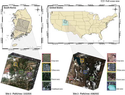
Two experimental areas were selected: the region within South Korea corresponding to the worldwide reference system 2 (WRS-2) path 115, row 35, and Salt Lake City in Utah, the United States, corresponding to path 38, row 32. For convenience, we designated the region in South Korea as Site 1 and the Salt Lake City area in the United States as Site 2. Both of these regions have a variety of environmental conditions and land coverage types, including urban, cropland, forests, water bodies, and barren land. Additionally, both areas are geographically located in the mid-latitude temperate climate zone, resulting in distinct four seasons. Consequently, images that contain clouds in varying proportions can be obtained due to the local climates. In particular, during the summer season, cloud data can be collected due to the impact of the rainy season front. Furthermore, Site 2 encompasses a lake area that exhibits progressive changes over time, prompting us to assess the performance and robustness of the proposed method. The regions of interest displayed in Figure 1, consisting of crop, urban, forest, and combined sites containing multiple land cover types, were selected for analyzing the applicability of the proposed algorithm.

Figure 1. Experimental areas with diverse land cover types in South Korea and the United States (images shown from May 7, 2020, and July 4, 2022, respectively).

Multitemporal image datasets exhibit temporal variability on their surfaces caused by land cover changes, including urbanization, deforestation, and crop rotation. Moreover, seasonal changes can provide diverse reflectance values in satellite data, particularly during the rainy season, which causes significant cloud contamination (Cao et al. 2020). Therefore, we evaluated the applicability of the proposed method based on time-series imagery by considering time variables. Full-scene images acquired between 2013 and 2023 with diverse cloud ratios from 0% to 80% for both regions were selected. In this dataset, all images could be selected as the cloud target image for restoration.

3. Methods

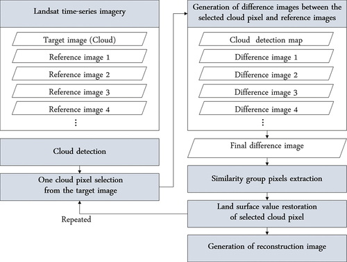
A flowchart of the proposed method is presented in Figure 2. In this study, we proposed criteria for detecting clouds from Landsat images using the QA band and developed a TSSG image restoration algorithm to remove the cloud regions. First, preprocessing, including image reflectivity calculation, was performed to apply this experiment to Landsat images, and the QA band was employed to detect cloud regions. This process established a criterion for identifying pixels that needed to be restored by detecting them as real clouds. Third, cloud regions were restored by the spectral similarity of multi-temporal images. Several reference images were selected to restore the removed cloud region from the cloud-masked image. The locations of pixels with similar spectrum values were extracted from reference images based on their spectral similarity to the cloud pixels to be reconstructed. The reflectance values of the ground beneath the clouds were predicted based on the pixels at the corresponding locations after substituting the extracted locations into the cloud images. This process was repeated for all pixels defined as clouds, and a reconstruction image without clouds was then created.

Figure 2. Workflow of the cloud detection and TSSG restoration algorithm.

3.1. Preprocessing

3.1.1. Reflectance image generation

The Landsat L1TP images provide digital number (DN) values of digitized radiance values without removing the sensor and solar effect. As a pre-processing step, DN values were converted to top-of-atmosphere (TOA) reflectance values. Equations for this process are provided by the United States Geological Survey (USGS), and all the required coefficients are obtained from the metadata of each image (Engebretson 2020). This process is represented as follows:

(1) ${\rho }_{\lambda }^{\prime }=M_{\rho }\times \mathit{D}{N}_{\mathit{cal}}+A_{\rho },$(1)

(2) ${\rho }_{\lambda }=\frac{{\rho }_{\lambda }^{\prime }}{\cos \left({\theta }_{\mathit{SZ}}\right)}=\frac{{\rho }_{\lambda }^{\prime }}{\sin \left({\theta }_{\mathit{SE}}\right)},$(2)

where ${\rho }_{\lambda }^{\prime }$ is the TOA spectral reflectance value without correction for the solar angle, $M_{\rho }$ is the reflectance multiplicative scaling factor for the band, $A_{\rho }$ is the reflectance additive scaling factor for the band, and $\mathit{D}{N}_{\mathit{cal}}$ is a pixel value in the DN image. Term ${\rho }_{\lambda }$ is the TOA reflectance value, ${\theta }_{\mathit{SE}}$ is the local solar zenith angle, and ${\theta }_{\mathit{SZ}}$ is the local scene center sun elevation angle.

3.1.2. Cloud detection

Landsat satellite images provide information on image quality, including cloud effects. Herein, we propose a quality information-based cloud detection technique to detect clouds on time-series images quickly and accurately. The LPGS produces pixel-level metadata that includes information on cloud masking, radiometric saturation, land characterization, and terrain occlusion. This metadata can be accessed by the user from the QA band, which includes pixel information on the surface, atmospheric, and sensor conditions at the time of acquisition. The quality index asserts water, snow, ice, clear, and cloud-related attributes, and it assigns bit values to each pixel as listed in Table 2. The cloud attributes provided by this QA information are primarily divided into two categories: “Cloud,” referring to thick clouds, and “Cirrus,” indicating thin clouds. Each attribute is reclassified based on the level of confidence, and there might be a possibility of overlap between the two attributes depending on the spectral state of cloud pixels. For example, a pixel may be classified as both low confidence in the cloud attribute and high confidence in the cirrus attribute. This necessitated the establishment of criteria for determining at what confidence level clouds should be considered. Therefore, a preliminary experiment was conducted to determine suitable criteria for precisely detecting cloud regions (Yun 2023).

Table 2. Pixel quality classification types from Landsat QA band.

Bit	Flag Description	Values
0	Fill	0 for image data 1 for fill data
1	Dilated cloud	0 for cloud is not dilated or no cloud 1 for cloud dilation
2	Cirrus	0 for cirrus confidence: no confidence level set or low confidence 1 for high confidence cirrus
3	Cloud	0 for cloud confidence is not high 1 for high confidence cloud
4	Cloud shadow	1 for cloud shadow confidence is not high 1 for high confidence cloud shadow
5	Snow	0 for snow/ice confidence is not high 1 for high confidence snow cover
6	Clear	0 if cloud or dilated cloud bits are set 1 if cloud and dilated cloud bits are not set
7	Water	0 for land or cloud 1 for water
8–9	Cloud confidence	00 for no confidence level set 01 low confidence 10 medium confidence 11 high confidence
10–11	Cloud shadow confidence	00 for no confidence level set 01 low confidence 10 reserved 11 high confidence
12–13	Snow/Ice confidence	00 for no confidence level set 01 low confidence 10 reserved 11 high confidence
14–15	Cirrus confidence	00 for no confidence level set 01 low confidence 10 reserved 11 high confidence

To establish the criteria, we generated five types of cloud detection maps based on the level of confidence in cloud and cirrus classes among attributes, as shown in Table 3. Subsequently, we conducted experiments to determine which map effectively detects cloud regions requiring restoration. For this purpose, 26 Landsat images with varying cloud cover percentages were collected, and Figure 3 illustrates sample images of the five cloud maps for one of these images. To assess the detection accuracy, the cloud reference masks initially created based on the QA band were refined using normalized difference water index (NDWI) and digital elevation model (DEM) (Yun 2023). Based on this reference data, all five cloud maps were applied to a total of 26 images to evaluate which one exhibited the highest accuracy. As a result, among cloud maps from A to E, cloud map D, which considers only cloud-high and cirrus-high attributes as cloud regions, exhibited the highest accuracy in most images. Based on these results, the cloud regions in all time-series satellite images were masked using the cloud map D, and during this step, the cloud masking maps generated as part of the detection process were employed to identify the areas requiring restoration. This process is more convenient and rapid than previous cloud detection methods such as threshold setting.

Figure 3. Sample images of cloud maps according to cloud confidence from QA image: (a) cloud RGB image acquired on April 4, 2020, in path/row 115/35, (b) cloud map A, (c) cloud map B, (d) cloud map C, (e) cloud map D, and (f) cloud map E.

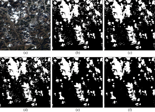
Table 3. Cloud maps based on the level of cloud confidence from QA image.

Cloud Map	Attributes
A	All attributes except “Clear”
B	“Cloud-high,” “Cloud-medium,” “Cloud-low,” “Cirrus-high,” “Cirrus-low”
C	“Cloud-high,” “Cloud-medium,” “Cirrus-high”
D	“Cloud-high,” “Cirrus-high”
E	“Cloud-high”

3.2. Time-series spectral similarity group

TSSG, a spatiotemporal-based approach, offers several significant differences when compared to the SSG method, primarily revolving around the incorporation of temporal information. Unlike SSG, which relies on a single reference image, the TSSG method employs multiple images as reference data, enhancing the reliability of the extracted information and reducing error ranges, ultimately resulting in improved accuracy. This approach allows for cloud restoration in target images, even when some reference data includes clouds. Additionally, images initially used as reference data can subsequently be repurposed as target images for restoration using other reference images. Through this method, continuous restoration can be achieved by utilizing both preceding and subsequent images within the established time-series database, contributing to the comprehensive reconstruction of all database images.

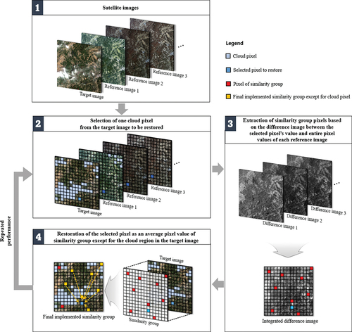
The TSSG algorithm employs time-series reference images to increase the reliability of position relations and precisely restore cloud regions using all bands. The basic concept of the TSSG method is described in Figure 4. First, in the time-series imagery database, some images close to the acquisition date of the cloud image are selected as time-series reference images. Second, a single cloud pixel to be restored is selected within the cloud pixels. Third, the corresponding pixels of each reference image are selected, which are located at the same location as the cloud pixel. In each reference image, a difference image is generated by subtracting the pixel value of the corresponding pixel from all pixel values within the reference image. The difference image for each reference image is calculated as follows:

(3) $\mathrm{\Delta }\mathit{I}\left(\mathit{i}\right)=\left[{\mathrm{\Delta }}_1\left(\mathit{i}\right),{\mathrm{\Delta }}_2\left(\mathit{i}\right),\dots {\mathrm{\Delta }}_n\left(\mathit{i}\right),\dots ,{\mathrm{\Delta }}_N\left(\mathit{i}\right)\right],$(3)

(4) ${\mathrm{\Delta }}_n\left(\mathit{i}\right)=R_n-R_n\left(\mathit{i}\right),$(4)

Figure 4. Proposed TSSG cloud regions restoration technique.

where $\mathit{i}$ is the selected cloud pixel in the target cloud image, $\mathit{N}$ is the number of reference images, ${\mathrm{\Delta }}_n\left(\mathit{i}\right)$ is the difference image with $\mathit{n}$-th reference images ($\mathit{n}=1,\dots ,\mathit{N}$), and $\mathrm{\Delta }\mathit{I}\left(\mathit{i}\right)$ indicates a group of difference images for all reference images related to the cloud pixel $\mathit{i}$. Term $R_n$ is the $\mathit{n}$-th reference image, and $R_n\left(\mathit{i}\right)$ indicates the corresponding pixel value of the $\mathit{n}$-th reference image, which has the same location as the cloud pixel $\mathit{i}$ in the target image.

After generating $\mathit{N}$ difference images, these are combined into one integrated difference image as follows:

(5) $\overline{\mathrm{\Delta }I\left(i\right)}=\sqrt{\frac{{\sum }_{n=1}^N{\left({\mathrm{\Delta }}_n\left(\mathit{i}\right)\right)}^2}{\mathit{N}}},$(5)

where $\overline{\mathrm{\Delta }I\left(i\right)}$ denotes the final integrated difference image.

The similarity group, which are pixels having similar pixel values with the pixel $\mathit{i}$, are then determined. This can be calculated by determining the low values in the integrated difference image $\overline{\mathrm{\Delta }I\left(i\right)}$. All pixels in the integrated difference image are sorted in ascending order, after which the values close to zero are identified as similarity group pixels.

After identifying the similarity group pixels, they are transferred from the integrated difference image to the cloud image. The mean value of those pixels in the cloud image (where they are not included in the cloud region) is then calculated and used as a restoration value for cloud pixel $\mathit{i}$. Let us assume that $\mathit{M}$ pixels are extracted as the TSSG and are not in the cloud region. Then, the substitute value can be estimated as follows:

(6) $\widehat{\mathit{I}\left(\mathit{\iota }\right)}=\frac{{\sum }_{m=1}^M\mathit{TSS}{G}_m}{\mathit{M}},$(6)

where $\widehat{\mathit{I}\left(\mathit{\iota }\right)}$ is the substitute value, which is the average of the values in the $\mathit{TSSG}$ pixels.

This process is repeated for all pixels in the cloud region. To improve the restoration result, unlike the general SSG method that extracts the common spectral similar pixels for all the bands, the TSSG method extracted them for each band individually. The proposed TSSG algorithm (Algorithm 1) is summarized as follows:

Table

Algorithm 1. TSSG cloud regions restoration method

Require: Pre-processed time-series satellite imagery dataset D. Select the target cloud image $\mathit{I}$ and number of $\mathit{N}$ reference images $R_n$ $\left(\mathit{n}=1,\dots ,\mathit{N}\right)$ from D. Main algorithm 1: Select one cloud pixel $\mathit{i}$ in $\mathit{I}$ to be restored. 2: Generate difference image between pixel value $\mathit{i}$ in reference image and entire reference image by Equation (3)(3) $\mathrm{\Delta }\mathit{I}\left(\mathit{i}\right)=\left[{\mathrm{\Delta }}_1\left(\mathit{i}\right),{\mathrm{\Delta }}_2\left(\mathit{i}\right),\dots {\mathrm{\Delta }}_n\left(\mathit{i}\right),\dots ,{\mathrm{\Delta }}_N\left(\mathit{i}\right)\right],$(3) , (4(4) ${\mathrm{\Delta }}_n\left(\mathit{i}\right)=R_n-R_n\left(\mathit{i}\right),$(4) ). 3: Generate integrated difference value image to extract similarity group using Equation (5)(5) $\overline{\mathrm{\Delta }I\left(i\right)}=\sqrt{\frac{{\sum }_{n=1}^N{\left({\mathrm{\Delta }}_n\left(\mathit{i}\right)\right)}^2}{\mathit{N}}},$(5) . 4: Extract time-series spectral similarity group pixels using integrated difference image. 5: Restore the pixel value of $\mathit{i}$ using similarity group pixels located in non-cloud region by Equation (6)(6) $\widehat{\mathit{I}\left(\mathit{\iota }\right)}=\frac{{\sum }_{m=1}^M\mathit{TSS}{G}_m}{\mathit{M}},$(6) . 6: Repeat for all cloud pixels and all bands of the target image. Output: Image that restored cloud regions

3.3. Accuracy assessment

Due to the absence of a ground truth image in cloud-covered regions, a comparison of the land-cover classification results before and after restoring the image is typically utilized for assessing image restoration techniques (Kim et al. 2014). However, assessing and comparing the classification-based evaluations from a quantitative perspective is difficult. In this study, to estimate the algorithm quantitatively, a cloud simulation image was generated from a non-cloud image by masking some pixels as cloud areas. Using the original image before cloud pixel generation as a reference image, the performance of the restoration method was evaluated by calculating the accuracy of the images obtained from the reconstruction of the cloud simulation image. In a subsequent step, the results of applying the proposed algorithm to the actual cloud data were examined through visual analytics and image classification. A comparative evaluation with the SSG method also demonstrated the applicability of the proposed method.

In this study, we selected and computed the following evaluation indices (Table 4) for a quantitative assessment of the image restoration algorithm: the peak signal-to-noise ratio (PSNR), structural similarity index (SSIM), mean absolute percentage error (MAPE), and normalized root mean square error (NRMSE). The mean square error (MSE) is an index used to measure the accuracy of an estimate by averaging the squared differences between the actual and substitute values and is employed in the calculation of PSNR. The PSNR index is used to assess the loss of quality information from an image, where a lower loss is expressed as a higher value (Elbadawy, El-Sakka, and Kamel 1998). The SSIM represents the degree of similarity between two images using a numerical range between 0 and + 1, where a higher value indicates increased their structural information similarity (Z. Wang et al. 2004). It was developed to address some of the limitations of traditional image similarity metrics (such as MSE and PSNR) that might not always conform to the human visual perception of image quality. The MAPE represents the error ratio, which determines the relative proportional error compared to the actual value by dividing the difference between the actual and alternative values (Makridakis et al. 1982). Because the degree of error is expressed as a percentage value, performance can be intuitively evaluated. Finally, the NRMSE is an evaluation index that normalizes the error to the average value of the measured values and is suitable for expressing precision.

Table 4. Equation of indices for evaluating the accuracy of cloud region restoration.

Index	Equation
NRMSE (Normalized Root Mean Square Error)	$\mathit{NRMSE}\left(I_r,I_p\right)=\frac{1}{\overline{I_r}}\sqrt{\frac{{\sum }_{I_r{I}_p}{\left(I_r-I_p\right)}^2}{I_r{I}_p}}$
MAPE (Mean Absolute Percentage Error)	$\mathrm{MAPE}($$I_r,I_p)=\frac{{\sum }_{{\mathit{I}}_{\mathit{width}},I_{\mathit{height}}}\left|\frac{I_r-I_p}{I_r}\right|}{I_{\mathit{width}}{I}_{\mathit{height}}}\times 100$
PSNR (Peak Signal-to-Noise Ratio)	$\mathit{PSNR}\left(I_r,I_p\right)=10{log}_{10}\frac{{\left(2^n-1\right)}^2}{\mathit{MSE}\left(I_r,I_p\right)}$ $\mathit{MSE}\left(I_r,I_p\right)=\frac{{\sum }_{I_r{I}_p}{\left(I_r-I_p\right)}^2}{I_r{I}_p}$
SSIM (Structural Similarity Index Measure)	$\mathit{SSIM}\left(I_r,I_p\right)=\mathit{l}\left(I_r,I_p\right)\mathit{c}\left(I_r,I_p\right)\mathit{s}\left(I_r,I_p\right)$ $\mathit{l}\left(I_r,I_p\right)=\frac{2{\mu }_{I_r}{\mu }_{I_p}+C_1}{{\mu }_{I_r}^2+{\mu }_{I_p}^2+C_1},\mathit{c}\left(I_r,I_p\right)=\frac{2{\sigma }_{I_r}{\sigma }_{I_p}+C_2}{{\sigma }_{I_r}^2+{\sigma }_{I_p}^2+C_2},\mathit{s}\left(I_r,I_p\right)=\frac{{\sigma }_{I_r{I}_p}+C_3}{{\sigma }_{I_r}{\sigma }_{I_p}+C_3}$

$I_r$= reference image, $I_p$= reconstruction image, $I_{\mathit{width}}$= width of image(s), $I_{\mathit{height}}$= height of image(s)

$C_1$, $C_2$, and $C_3$= stabilizing constants, $\mathit{n}$ = bit-depth of the image

4. Results

4.1. Performance of the TSSG algorithm

Cloud simulation images were generated for Sites 1 and 2 to enable a quantitative evaluation. Based on this evaluation, a comparative analysis was performed on the cloud reconstruction images obtained using the TSSG and SSG algorithms. As indicated in Table 5, the accuracy evaluation results of the TSSG method consistently exhibited higher accuracy across all metrics compared to the SSG algorithm. The SSIM values were 0.8927 for Site 1 and 0.8859 for Site 2, while the PSNR values were 52.1979 for Site 1 and 40.3423 for Site 2. These findings clearly demonstrated the superior performance of the TSSG method in comparison to the SSG algorithm. The proposed method achieved NRMSE and MAPE indices of 0.0184 and 0.2249% for Site 1 and 0.0313 and 4.3484% for Site 2, respectively. The method we propose yields much lower error values compared to the SSG method and demonstrates superior performance for several reasons. First, the number of reference images was increased to ensure the high reliability of the location information used for calculating the restoration value. Additionally, the similarity group pixels were extracted independently for each band to obtain accurate values for the pixels. Figures 5 and 6 display the reconstruction images produced by the TSSG algorithm. These images include the cloud simulation image, the original image, and the SSG result, showing various land cover types such as crop sites, urban areas, forested regions, and combined sites in both Site 1 and Site 2. The reconstructed images were visually evaluated based on the TSSG algorithm. The proposed method exhibited excellent restoration performance for all land cover sites. Moreover, the cloud regions of the reconstruction images tended to resemble the original images for every pixel, regardless of the heterogeneity of land cover. In addition, it was confirmed that the crop site and forest site, which are directly affected by seasonal differences, were restored equally to the radiometric characteristics of the original image. In the reconstruction images using SSG, the shape of the land surface can be distinguished, but it generally exhibited a lower contrast ratio compared to surrounding pixels, making it challenging to create a natural-looking restoration image. In comparison, the proposed method yielded a well-reconstructed image that was indistinguishable from the original image without a representative boundary between the cloud and non-cloud regions.Figure 7

Table 5. SSIM, PSNR, NRMSE, and MAPE values of SSG and TSSG algorithms-based reconstruction images at two sites.

	Site 1 (South Korea)				Site 2 (USA)
	SSIM	PSNR	NRMSE	MAPE	SSIM	PSNR	NRMSE	MAPE
Cloud image	0.1536	28.4584	0.2727	6.2482	0.0457	23.7896	0.1738	13.5678
SSG	0.5241	40.7478	0.0682	1.2664	0.4485	28.6493	0.1275	18.9369
TSSG	0.8927	52.1979	0.0184	0.2249	0.8859	40.3423	0.0313	4.3484

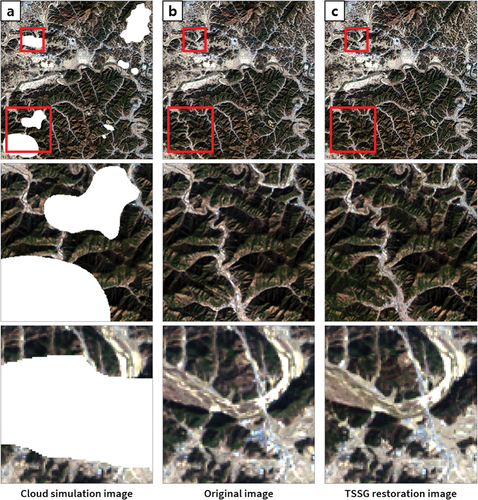
Figure 5. Visual comparison examples of true-color restoration results in site 1, South Korea. The second and third lines of each figure depict enlarged images of the red rectangle regions: (a) Landsat 8 original cloud-free images on March 20, 2020, (b) cloud simulation images, (c) restored images using SSG, and (d) restored images using proposed TSSG (Landsat 8 on November 29, 2019 and April 5, 2020 were used for restoration as reference data).

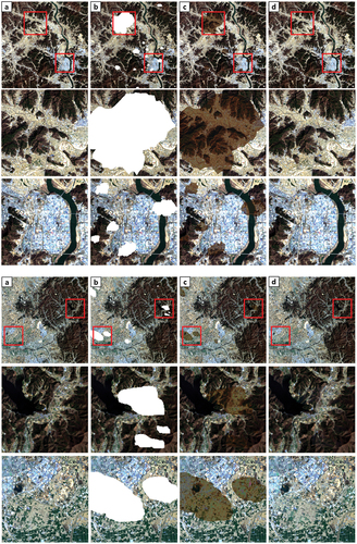
Figure 6a. Visual comparison examples of true-color restoration results in site 2, USA. The second and third lines of each figure depict enlarged images of the red rectangle regions: (a) Landsat 8 original cloud-free images on September 25, 2023, (b) cloud simulation images, (c) restored images using SSG, and (d) restored images using proposed TSSG (Landsat 9 images on August 29, 2022 and October 19, 2023 were used for restoration as reference data).

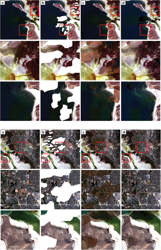
Figure 6b. (Continued)

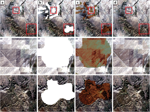
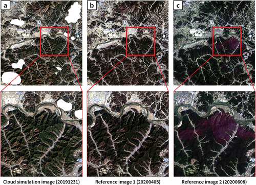
Figure 7a. Visual comparison examples of restoration results. The second and third lines of each figure depict enlarged images of the yellow rectangle region: (a) Landsat 8 images on March 4, 2020, South Korea, (b) Landsat 8 images on December 17, 2020, South Korea, (c) Landsat 9 images on April 3, 2022, USA.

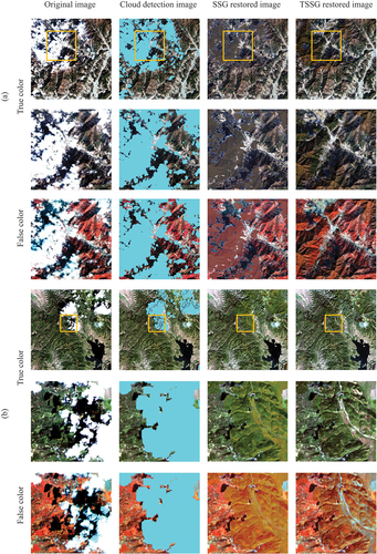
Figure 7b. (Continued)

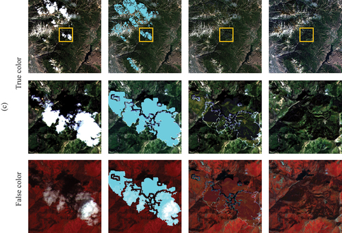
Figure 8. Experimental true-color images from Landsat 8 with abrupt land cover change by wildfire in South Korea. The second lines of each figure depict enlarged images of the red rectangle regions: (a) cloud simulation image on 31 December 2019, (b) first reference image on 5 April 2020, (c) second reference image on 8 June 2020 including regions affected by wildfires.

5. Discussion

5.1. Performance analysis of TSSG parameters

The TSSG technique offers the flexibility for fine-tuning through multiple parameter adjustments in the restoration process. To optimize the performance of the proposed TSSG method, a comprehensive evaluation of several parameters was conducted. Specifically, the optimization process encompassed variables such as the number of reference images, the proportion of cloud coverage within these reference images, and the ratio of similarity group pixels for restoration. The number of reference images pertains to the extent of temporal information employed during the application of the TSSG technique. In order to ascertain the optimal number of reference images yielding enhanced quality in the reconstructed images, a comparative experiment was conducted. This analysis involved systematically varying the number of reference images within the range of 1 to 8. The ensuing analysis examines the influence of the quantity of time-series information on the reliability of the restored imagery. The cloud cover percentage parameter of the reference image served as an experimental metric to assess the capability of the proposed method to ensure a certain level of accuracy, even when using reference images that contained cloud cover. Accordingly, this parameter helped when examining the method’s robustness and efficiency under challenging atmospheric conditions. The similarity group pixel ratio for reconstruction was used as a parameter to assess the range within which minimal errors were encountered and to determine the performance characteristics. This empirical examination is essential to prevent errors occurring due to excessive pixel utilization. Since the parameters were changed in all cases, each reconstructed image was evaluated to determine the applicability of the parameters. To assess the effect of each parameter, the dependent and independent variables should be separated during the experiments. All variables were fixed in the experiment design to test for optimal parameters analysis, except the parameters to be tested.

5.1.1. Performance analysis of TSSG based on number of reference images

An image restoration procedure based on reference 1 1–8 was conducted to determine the optimal number of reference images required to extract location information from similar pixels. The reference images close to the acquisition date of the cloud target image were preferentially selected. Using the indices referenced in Section 4.1, the accuracy of the experiment results was compared and evaluated. The reconstructed images based on the two reference images exhibited the highest accuracy at Sites 1 and 2, as listed in Table 6. The SSIM values for Site 1 were 0.8927 and for Site 2 were 0.8859, while the PSNR values for Site 1 were 52.1979 and for Site 2 were 40.3423, resulting in the highest image quality. In comparison, the NRMSE values for Site 1 were 0.0184 and for Site 2 were 0.0313, and the MAPE values for Site 1 were 0.2249 and for Site 2 were 4.3484, indicating the lowest error values. Conversely, the accuracy was lowest for the reconstructed images derived from a single image. In the case of three or more images being used as reference images, the accuracy gradually decreased with an increase in the number of images. In this regard, the location of similar pixels could be identified more reliably when two reference images were available. Furthermore, regardless of the number of reference images used, all the TSSG cases produced higher accuracy than the SSG accuracy values presented in Table 5. Therefore, the number of reference images could be adapted to suit the characteristics of the selected regions in satellite images.

Table 6. SSIM, PSNR, NRMSE, and MAPE values of TSSG reconstructed images according to the number of reference images in two sites.

		Site 1				Site 2
		SSIM	PSNR	NRMSE	MAPE	SSIM	PSNR	NRMSE	MAPE
Number of reference images for TSSG	1	0.6634	46.9554	0.0344	0.5949	0.6390	31.6004	0.0539	7.7915
	2	0.8927	52.1979	0.0184	0.2249	0.8859	40.3423	0.0313	4.3484
	3	0.8913	52.0338	0.0187	0.2253	0.8844	39.9858	0.0326	4.345
	4	0.8864	51.8289	0.0192	0.2337	0.8632	38.8170	0.0378	4.8906
	5	0.8791	51.4813	0.0199	0.2453	0.8543	38.4666	0.0393	4.9886
	6	0.8809	51.6476	0.0195	0.2405	0.8463	37.9409	0.0415	5.1762
	7	0.8717	51.2304	0.0204	0.2524	0.8519	38.1547	0.0406	5.1852
	8	0.8717	51.2246	0.0204	0.2524	0.8350	36.3171	0.0481	5.6986

5.1.2. Performance analysis of TSSG based on cloud ratio of reference images

Two reference images were used to analyze the effect of cloud ratio on the overall accuracy. Reference images with cloud ratios of 1%, 5%, 10%, 20%, 30%, 40%, and 50% were selected (Table 7). At a cloud coverage ratio of 1%, both Site 1 and Site 2 achieved the highest level of accuracy across all metrics. This important trend persisted, with the 10% cloud coverage representing the second-highest level of accuracy, notably through the SSIM and NRMSE ratios. The accuracy values gradually decreased with an increasing cloud ratio, but the exponential values between 1% and 20% remained similar, demonstrating NRMSE values below 0.1, suggesting that cloud ratios below 20% had a limited impact on the restoration quality. Beyond a 20% ratio, the deviation sharply increased. Nevertheless, when examining the evaluation results for cloud ratios of 30%, 40%, and 50% specifically, it is evident that at Site 1, PSNR remained around 40, and NRMSE was below 0.08, while at Site 2, PSNR stayed above 28, and NRMSE remained below 0.12 consistently. Furthermore, even at a reference image’s cloud ratio of 50%, the proposed TSSG method showed higher accuracy compared to existing SSG restoration techniques. This consistency provides practical evidence of the method’s superiority. Therefore, the proposed restoration method demonstrates the ability to generate highly accurate reconstructed images even when reference images contain a certain level of cloud coverage.

Table 7. SSIM, PSNR, NRMSE, and MAPE values of TSSG reconstructed images according to the cloud ratio of reference images in two sites.

		Site 1				Site 2
		SSIM	PSNR	NRMSE	MAPE	SSIM	PSNR	NRMSE	MAPE
Cloud ratio of reference image for TSSG	1%	0.8724	51.2573	0.0204	0.2641	0.8859	40.3423	0.0313	4.3484
	5%	0.4592	44.6118	0.0479	0.9966	0.7083	35.0059	0.0582	7.2984
	10%	0.6425	45.5739	0.0390	0.5668	0.7835	35.7543	0.0536	7.3260
	20%	0.5992	46.6018	0.0351	0.6327	0.5569	32.9797	0.0725	9.8077
	30%	0.4041	43.1996	0.0533	0.9431	0.2642	29.6447	0.1068	15.4000
	40%	0.4225	39.8299	0.0772	1.6024	0.2256	29.8215	0.1043	15.5360
	50%	0.2967	40.8756	0.0682	1.4250	0.2319	28.9130	0.1167	16.8713

5.1.3. Performance analysis of TSSG based on spectral similarity group pixel ratio

Two reference images with cloud ratios of less than 1% were used to evaluate the results of the image restoration under the ratio of the similarity group pixel over the entire image pixels. The identification of similarity group pixels involved the detection of pixels with a minimal difference close to zero in the final difference image, as described in Section 3.2. At this point, the number of similarity group pixels to be extracted should be specified by the user. Consequently, this study attempted to determine how much of the similarity group pixel ratio should be taken from the entire image to find the optimal number of similarity group pixels. The extracted ratio of the similarity group over entire image pixels were composed of 0.05%, 0.1%, 0.2%, 0.3%, 0.5%, 1%, 2%, and 3%. A performance evaluation index was calculated based on the reconstructed image (Table 8). For Site 1, high accuracy was primarily observed at a 0.3% cloud ratio, whereas Site 2 demonstrated proficient results with a 0.1% cloud ratio. However, there was no single ratio uniformly identified as optimal by all metrics, and the results across all conceivable similarity group pixel ratio showed a comparable level of quality. Compared with the SSG result in Table 5, the accuracy of all ratios was improved. Therefore, the similarity group pixel ratio for the entire image did not show a significant change in decimal percentages and had no notable impact on the overall TSSG performance. Therefore, highly accurate results can be achieved even when the ratio is changed within 3%, according to the speed and time characteristics of the algorithm.

Table 8. SSIM, PSNR, NRMSE, and MAPE values of TSSG reconstructed images according to the similarity group pixel ratios in two sites.

		Site 1				Site 2
		SSIM	PSNR	NRMSE	MAPE	SSIM	PSNR	NRMSE	MAPE
Similarity group pixel ratios	0.05%	0.8646	52.0377	0.0186	0.2510	0.8684	40.8139	0.0296	3.9661
	0.1%	0.8717	52.0316	0.0186	0.2455	0.8759	40.8387	0.0295	3.9900
	0.2%	0.8753	51.9726	0.0186	0.2434	0.8808	40.7260	0.0299	4.0851
	0.3%	0.8766	52.0682	0.0184	0.2437	0.8831	40.5831	0.0304	4.1844
	0.5%	0.8772	51.9823	0.0185	0.2461	0.8859	40.3423	0.0313	4.3484
	1%	0.8764	51.5318	0.0194	0.2527	0.8893	39.9709	0.0327	4.6027
	2%	0.8733	50.8080	0.0211	0.2653	0.8913	39.6146	0.0340	4.8452
	3%	0.8699	50.2854	0.0224	0.2828	0.8865	39.4214	0.0398	4.9981

5.2. Advantages of TSSG compared to previous restoration method

To further assess the cloud restoration performance of the TSSG method, we conducted a comparison analysis of the band-wise restoration results with SSG method for the evaluation regions of Site 1 in South Korea and Site 2 in the USA. The restoration outcomes from band 1 (Coastal aerosol) to band 7 (SWIR 2) images were evaluated using the SSIM, PSNR, NRMSE, and MAPE metrics. As presented in Tables 9 and 10, TSSG method demonstrated superior image quality and reduced errors in all evaluation metrics for both Site 1 and Site 2 compared to SSG.

Table 9. Comparisons of SSIM, PSNR, NRMSE, and MAPE between SSG and TSSG cloud restoration results for site 1 (South Korea).

Site 1 (South Korea)	SSG				TSSG
	SSIM	PSNR	NRMSE	MAPE	SSIM	PSNR	NRMSE	MAPE
Coastal aerosol	0.5780	43.7221	0.0483	0.7713	0.9005	57.0121	0.0105	0.0884
Blue	0.5331	42.4572	0.0647	1.0117	0.8979	55.4625	0.0145	0.1467
Green	0.5181	41.5463	0.0834	1.2069	0.8997	54.4963	0.0188	0.1897
Red	0.5619	40.7601	0.0887	1.2007	0.9002	52.9768	0.0217	0.2475
NIR	0.4472	40.6704	0.0480	1.1754	0.8731	49.6443	0.0171	0.2750
SWIR1	0.4654	38.2528	0.0584	1.6079	0.8842	47.5507	0.0200	0.2878
SWIR2	0.5650	37.8260	0.0859	1.8906	0.8936	48.2429	0.0259	0.3394

Table 10. Comparisons of SSIM, PSNR, NRMSE, and MAPE between SSG and TSSG cloud restoration results for site 2 (USA).

Site 2 (USA)	SSG				TSSG
	SSIM	PSNR	NRMSE	MAPE	SSIM	PSNR	NRMSE	MAPE
Coastal aerosol	0.4650	29.7950	0.2184	20.5951	0.8722	44.4286	0.0405	3.4776
Blue	0.5828	29.8142	0.1802	22.7051	0.9045	45.0347	0.0312	3.534
Green	0.6481	29.5820	0.1154	19.1172	0.8958	42.6592	0.0256	3.8571
Red	0.3957	30.7042	0.0885	11.6117	0.8929	41.5162	0.0255	4.6072
NIR	0.2707	28.8399	0.0659	13.4713	0.8685	36.2856	0.0280	4.7754
SWIR1	0.4810	25.4316	0.1133	18.9369	0.8720	35.1798	0.0369	4.3484
SWIR2	0.2963	26.3788	0.1109	26.1215	0.8954	37.2922	0.0316	5.8395

Furthermore, through this experiment, TSSG exhibited several improvements compared to prior research. First, TSSG showed low dependence on the reference image selection process for restoration, as it easily selects reference images. By utilizing information only from areas excluding cloud regions, TSSG produced appropriate restoration results even when the quality of the reference image was low and clouds were present. In addition, the utilization of imagery containing abrupt changes as reference images has been confirmed. Figure 8 presents additional experimental images conducted to demonstrate this point, particularly focusing on the image corresponding to reference 2 2 in Figure 8(c), which encompasses areas affected by wildfires that occurred on 1 May 2020. Despite not specifically screening or excluding the wildfire-damaged regions before applying TSSG, the restoration results, as depicted in Figure 9, exhibit restored images visually similar to the original images prior to the simulated cloud cover. The second improvement is that TSSG possesses robust features against seasonal variations. The restoration results in Table 9 for Site 1, referencing images from 20 March 2020, and 5 April 2020, for the 29 November 2019 cloud image, yielded higher accuracy restoration results compared to SSG. Additionally, Site 2 in Table 10 utilized images from 25 September 2023, and 19 October 2023, as reference images for the 29 August 2022 cloud image, demonstrating high restoration performance despite a time gap of over a year. These findings highlight the efficacy of the TSSG algorithm in cloud restoration, showcasing its advantages and performance to variations in reference image quality, and temporal differences.

Figure 9. The performance of TSSG using wildfire-affected image as supplementary material. The second and third lines of each figure depict enlarged images of the red rectangle regions: (a) cloud simulation images, (b) original cloud-free images, (c) restored images using proposed TSSG.

5.3. Limitations of TSSG

The proposed restoration algorithm demonstrates flexible applicability and high performance. It robustly responds to seasonal changes in reference images and can utilize reference images even in scenes containing clouds, showcasing its versatility. However, challenges arise in rapidly changing regions, such as those affected by wildfires or floods, where the likelihood of errors increases. In the previous section, it was mentioned that images containing changes due to wildfires can be used as reference images. However, if the change areas themselves are obscured by clouds, the TSSG approach may find it challenging to predict such changes. Therefore, images capturing drastic changes due to disasters may prove challenging for restoration. Additionally, it faces difficulties in providing accurate values for snowy or icy regions and polar areas. The algorithm faces constraints in abrupt changes, as evidenced by a general increase in average brightness values at snow regions. Lastly, with an increase in the cloud cover ratio in the reference image, achieving optimal results becomes more demanding. This limitation stems from the nature of the proposed method, which relies on information from areas excluding cloud regions. A higher cloud cover ratio in the reference image implies a reduction in available information, complicating the attainment of optimal results. Despite these limitations, the algorithm excels in regions like mountains, tropical forests, lakes, seas, and other water bodies. It consistently delivers optimal restoration results in extensive, homogeneous land cover areas, addressing a common drawback highlighted in prior research.

6. Conclusion

The purpose of this study was to effectively restore cloud-covered areas to enhance the utility of cloud-covered optical satellite imagery. The proposed algorithm used Landsat QA band attributes to enable precise cloud detection. The TSSG algorithm utilizes time series images as reference data to remove cloud-affected areas and generate high quality reconstructed images. The method was evaluated using both simulated and real cloud-covered satellite images. The quantitative evaluation results based on cloud simulation imagery indicated an accuracy improvement compared to other restoration techniques. Additionally, it visually confirmed that the TSSG method can be applied effectively to real cloud images that exhibit irregular cloud boundaries and radiometric variability. To optimize the TSSG method’s performance and demonstrate its robustness, three parameters were analyzed in detail: the number of reference images, the ratio of similarity group pixels, and the cloud ratio in reference images. One of the advantages of the proposed algorithm is that the proposed method simplified the selection of reference images since cloud-contaminated images can also be used as references, eliminating a limitation noted in the previous research. Moreover, it can account for seasonal variations and generate high-quality restored images even with time lags of more than a year. The proposed TSSG can be seamlessly applied to images from Landsat 5, Landsat 7, and Landsat 8–9. Moreover, the algorithm is applicable to Sentinel satellite images by replacing the cloud detection step with cloud screening using usable data mask (UDM) information provided for the regions requiring restoration. Consequently, the subsequent image restoration process of TSSG can be applied without modification. This implies that if a satellite provides cloud information through UDM or ARD products, accessing this algorithm becomes straightforward. Even if not, as long as there is a reliable method to distinguish obstructed cloud pixels, the proposed algorithm allows for image restoration.

While the proposed method shows the potential to enhance the restoration quality of cloud-covered satellite imagery, it has limitations. For images with abrupt and significant changes, such as wildfires or floods, generating high-quality restored images can be challenging due to the difficulty of collecting reliable similarity group. Additionally, it was observed that obtaining ideal results becomes difficult when the cloud-covered ratio in the reference images exceeds 20% of the entire image. Further studies focusing on solving such limitations will be our future work by assigning weights according to the reliability of reference images or conducting more experiments in various cloud-covered conditions.

Credit author statement

Yerin Yun: Conceptualization, Methodology, Software, Investigation, Writing-Original Draft preparation. Jinha Jung: Validation, Writing – Reviewing and Editing. Youkyung Han: Conceptualization, Writing – Reviewing and Editing, Supervision, Project administration, Funding acquisition.

Acknowledgments

The study was supported as part of the National Research Foundation of Korea (2021R1A2C2093671) project by the Korean government.

Disclosure statement

The authors declare that they have no known competing financial interests or personal relationships that could have appeared to influence the work reported in this paper.

Data availability statement

The dataset will be open to public via https://github.com/YerinYun17/TSSG.

Additional information

Funding

The study was supported as part of the National Research Foundation of Korea (2021R1A2C2093671) project by the Korean government.

References

- Bai, B., Y. Tan, K. Zhou, G. Donchyts, A. Haag, and A. H. Weerts. 2022. “Time-Series Surface Water Gap Filling Based on Spatiotemporal Neighbourhood Similarity.” International Journal of Applied Earth Observation and Geoinformation 112:102882. https://doi.org/10.1016/j.jag.2022.102882.
- Brown, A. J., and Y. Xie. 2012. “Symmetry Relations Revealed in Mueller Matrix Hemispherical Maps.” Journal of Quantitative Spectroscopy and Radiative Transfer 113 (8): 644–21. https://doi.org/10.1016/j.jqsrt.2012.01.008.
- Candra, D. S., S. Phinn, and P. Scarth. 2016. “Cloud and Cloud Shadow Masking using Multi-temporal Cloud Masking Algorithm in Tropical Environmental.” International Archives of the Photogrammetry, Remote Sensing and Spatial Information Sciences XLI-B2:95–100. https://doi.org/10.5194/isprs-archives-XLI-B2-95-2016.
- Cao, R., Y. Chen, J. Chen, X. Zhu, and M. Shen. 2020. “Thick Cloud Removal in Landsat Images Based on Autoregression of Landsat Time-Series Data.” Remote Sensing of Environment 249:112001. https://doi.org/10.1016/j.rse.2020.112001.
- Chen, B., B. Huang, L. Chen, and B. Xu. 2016. “Spatially and Temporally Weighted Regression: A Novel Method to Produce Continuous Cloud-Free Landsat Imagery.” IEEE Transactions on Geoscience and Remote Sensing 55 (1): 27–37. https://doi.org/10.1109/TGRS.2016.2580576.
- Elbadawy, O., M. R. El-Sakka, and M. S. Kamel 1998. “An Information Theoretic Image-Quality Measure.” In Conference Proceedings. IEEE Canadian Conference on Electrical and Computer Engineering, 25-28 May 1998, Waterloo, ON, Canada 1:169–172.
- Engebretson, C. 2020. “Landsat 8–9 Operational Land Imager (OLI)—Thermal Infrared Sensor (TIRS) Collection 2 Level 1 (L1) Data Format Control Book (DFCB).” Department Inter US Geological Survey. https://www.usgs.gov/media/files/landsat-8-9-olitirs-collection-2-level-1-data-format-control-book.
- Gao, J., Q. Yuan, J. Li, H. Zhang, and X. Su. 2020. “Cloud Removal with Fusion of High Resolution Optical and SAR Images Using Generative Adversarial Networks.” Remote Sensing 12 (1): 191. https://doi.org/10.3390/rs12010191.
- Gomez, L., J. Amoros, G. Mateo, J. Munoz, and G. Camps. 2017. “Cloud Masking and Removal in Remote Sensing Image Time Series.” Journal of Applied Remote Sensing 11 (1): 015005. https://doi.org/10.1117/1.JRS.11.015005.
- Huang, C., N. Thomas, S. N. Goward, J. G. Masek, Z. Zhu, J. R. Townshend, and J. E. Vogelmann. 2010. “Automated Masking of Cloud and Cloud Shadow for Forest Change Analysis Using Landsat Images.” International Journal of Remote Sensing 31 (20): 5449–5464. https://doi.org/10.1080/01431160903369642.
- Ivanchuk, N., P. Kogut, and P. Martyniuk. 2023. “Data Fusion of Satellite Imagery for Generation of Daily Cloud Free Images at High Resolution Level.” arXiv Preprint arXiv. https://doi.org/10.48550/arXiv.2302.12495.
- Jin, S., C. Homer, L. Yang, G. Xian, J. Fry, P. Danielson, and P. A. Townsend. 2013. “Automated Cloud and Shadow Detection and Filling Using Two-Date Landsat Imagery in the USA.” International Journal of Remote Sensing 34 (5): 1540–1560. https://doi.org/10.1080/01431161.2012.720045.
- Kang, S., Y. Choi, and J. Choi. 2021. “Restoration of Missing Patterns on Satellite Infrared Sea Surface Temperature Images Due to Cloud Coverage Using Deep Generative Inpainting Network.” Journal of Marine Science and Engineering 9 (3): 310. https://doi.org/10.3390/jmse9030310.
- Kim, B., Y. Kim, Y. Han, W. Choi, and Y. Kim. 2014. “Fully Automated Generation of Cloud-Free Imagery Using Landsat-8.” Journal of the Korean Society of Surveying, Geodesy, Photogrammetry and Cartography 32 (2): 133–142. https://doi.org/10.7848/ksgpc.2014.32.2.133.
- Konik, M., M. Kowalewski, K. Bradtke, and M. Darecki. 2019. “The Operational Method of Filling Information Gaps in Satellite Imagery Using Numerical Models.” International Journal of Applied Earth Observation and Geoinformation 75:68–82. https://doi.org/10.1016/j.jag.2018.09.002.
- Lee, M. H., E. J. Cheon, and Y. D. Eo. 2019. “Cloud Detection and Restoration of Landsat-8 Using STARFM.” Korean Journal of Remote Sensing 35 (5–2): 861–871. https://doi.org/10.7780/kjrs.2019.35.5.2.10.
- Li, W., Y. Li, D. Chen, and J. C. W. Chan. 2019. “Thin Cloud Removal with Residual Symmetrical Concatenation Network.” ISPRS Journal of Photogrammetry and Remote Sensing 153:137–150. https://doi.org/10.1016/j.isprsjprs.2019.05.003.
- Liu, H., B. Huang, and J. Cai. 2023. “Thick Cloud Removal Under Land Cover Changes Using Multisource Satellite Imagery and a Spatiotemporal Attention Network.” IEEE Transactions on Geoscience and Remote Sensing 61:1–18. https://doi.org/10.1109/TGRS.2023.3334492.
- Li, X., L. Wang, Q. Cheng, P. Wu, W. Gan, and L. Fang. 2019. “Cloud Removal in Remote Sensing Images Using Nonnegative Matrix Factorization and Error Correction.” ISPRS Journal of Photogrammetry and Remote Sensing 148:103–113. https://doi.org/10.1016/j.isprsjprs.2018.12.013.
- Maduskar, D., and N. Dube. 2021. “Navier–Stokes-based Image Inpainting for Restoration of Missing Data Due to Clouds.” In Innovations in Computational Intelligence and Computer Vision, edited by M. K. Sharma, V. S. Dhaka, T. Perumal, N. Dey, and J. M. R. S. Tavares, 497–505. Singapore: Springer. https://doi.org/10.1007/978-981-15-6067-5_56.
- Makridakis, S., A. Andersen, R. Carbone, R. Fildes, M. Hibon, R. Lewandowski, J. Newton, E. Parzen, and R. Winkler. 1982. “The Accuracy of Extrapolation (Time Series) Methods: Results of a Forecasting Competition.” Journal of Forecasting 1 (2): 111–153. https://doi.org/10.1002/for.3980010202.
- Mohajerani, S., T. A. Krammer, and P. Saeedi. 2018. “Cloud Detection Algorithm for Remote Sensing Images Using Fully Convolutional Neural Networks.” ArXiv Preprint. https://doi.org/10.48550/arXiv.1810.05782.
- Norris, J., R. Allen, A. Evan, M. Zelinka, C. O’Dell, and S. Klein. 2016. “Evidence for Climate Change in the Satellite Cloud Record.” Nature 536 (7614): 72–75. https://doi.org/10.1038/nature18273.
- Shen, H., X. Li, Q. Cheng, C. Zeng, G. Yang, H. Li, and L. Zhang. 2015. “Missing Information Reconstruction of Remote Sensing Data: A Technical Review.” IEEE Geoscience and Remote Sensing Magazine 3 (3): 61–85. https://doi.org/10.1109/MGRS.2015.2441912.
- Shen, Y., Y. Wang, H. Lv, and H. Li. 2015. “Removal of Thin Clouds Using Cirrus and QA Bands of Landsat-8.” Photogrammetric Engineering and Remote Sensing 81 (9): 721–731. https://doi.org/10.14358/PERS.81.9.721.
- Sun, L., X. Liu, Y. Yang, T. Chen, Q. Wang, and X. Zhou. 2018. “A Cloud Shadow Detection Method Combined with Cloud Height Iteration and Spectral Analysis for Landsat 8 OLI Data.” ISPRS Journal of Photogrammetry and Remote Sensing 138:193–207. https://doi.org/10.1016/j.isprsjprs.2018.02.016.
- Wang, Z., A. C. Bovik, H. R. Sheikh, and E. P. Simoncelli. 2004. “Image Quality Assessment: From Error Visibility to Structural Similarity.” IEEE Transactions on Image Processing 13 (4): 600–612. https://doi.org/10.1109/TIP.2003.819861.
- Wang, J., C. K. Lee, X. Zhu, R. Cao, Y. Gu, S. Wu, and J. Wu. 2022. “A New Object-Class Based Gap-Filling Method for PlanetScope Satellite Image Time Series.” Remote Sensing of Environment 280:113136. https://doi.org/10.1016/j.rse.2022.113136.
- Wang, J. L., X. L. Zhao, H. C. Li, K. X. Cao, J. Miao, and T. Z. Huang. 2023. “Unsupervised Domain Factorization Network for Thick Cloud Removal of Multi-Temporal Remotely Sensed Images.” IEEE Transactions on Geoscience and Remote Sensing 61:5405912. https://doi.org/10.1109/TGRS.2023.3303169.
- Wang, Z., D. Zhou, X. Li, L. Zhu, H. Gong, and Y. Ke. 2023. “Virtual Image-Based Cloud Removal for Landsat Images.” GIScience & Remote Sensing 60 (1): 2160411. https://doi.org/10.1080/15481603.2022.2160411.
- Xia, M., and K. Jia. 2022. “Reconstructing Missing Information of Remote Sensing Data Contaminated by Large and Thick Clouds Based on an Improved Multitemporal Dictionary Learning Method.” IEEE Transactions on Geoscience and Remote Sensing 60:1–14. https://doi.org/10.1109/TGRS.2021.3095067.
- Yang, G., H. Shen, L. Zhang, Z. He, and X. Li. 2015. “A Moving Weighted Harmonic Analysis Method for Reconstructing High-Quality SPOT Vegetation NDVI Time-Series Data.” IEEE Transactions on Geoscience and Remote Sensing 53 (11): 6008–6021. https://doi.org/10.1109/TGRS.2015.2431315.
- Yu, X., and D. J. Lary. 2021. “Cloud Detection Using an Ensemble of Pixel-Based Machine Learning Models Incorporating Unsupervised Classification.” Remote Sensing 13 (16): 3289. https://doi.org/10.3390/rs13163289.
- Yun, Y. 2023. “Cloud detection and image reconstruction from Landsat imagery based on time-series spectral similarity group.” Master’s thesis, Seoul National University of Science and Technology. http://www.dcollection.net/handler/snut/200000659928.
- Zhang, Q., Q. Yuan, C. Zeng, X. Li, and Y. Wei. 2018. “Missing Data Reconstruction in Remote Sensing Image with a Unified Spatial–Temporal–Spectral Deep Convolutional Neural Network.” IEEE Transactions on Geoscience and Remote Sensing 56 (8): 4274–4288. https://doi.org/10.1109/TGRS.2018.2810208.
- Zhou, Y. N., S. Wang, T. Wu, L. Feng, W. Wu, J. Luo, X. Zhang, and N. N. Yan. 2022. “For-Backward LSTM-Based Missing Data Reconstruction for Time-Series Landsat Images.” GIScience & Remote Sensing 59 (1): 410–430. https://doi.org/10.1080/15481603.2022.2031549.
- Zhu, Z., S. Qiu, B. He, and C. Deng. 2018. “Cloud and Cloud Shadow Detection for Landsat Images: The Fundamental Basis for Analyzing Landsat Time Series”. In Time Series Image/Data Generation, edited by Q. Weng, 3–23. 1st ed. Remote Sensing Time Series Image Processing Boca Raton, Florida, US: Taylor and Francis Group. https://doi.org/10.1201/9781315166636-1.
- Zhu, Z., and C. E. Woodcock. 2012. “Object-Based Cloud and Cloud Shadow Detection in Landsat Imagery.” Remote Sensing of Environment 118:83–94. https://doi.org/10.1016/j.rse.2011.10.028.