Process-based and geostationary meteorological satellite-enhanced dead fuel moisture content estimation

ABSTRACT

Dead fuel moisture content (DFMC) is essential for assessing wildfire danger, fire behavior, and fuel consumption. Several process-based models have been proposed to estimate DFMC. Previous studies have employed process-based models to estimate DFMC, solely relying on meteorological data obtained from meteorological stations. Satellite data can offer higher spatial resolution compared to meteorological data, with the potential to enhance the process-based DFMC estimates. Within this content, we aimed to improve the DFMC estimates by consideration of geostationary meteorological satellite-derived key variable (relative humility, RH) into the Fuel Stick Moisture Model (FSMM). The RH was derived from Himawari-8 geostationary satellite data, and other variables required by FSMM were obtained from Global Forecast System (GFS). As comparison, an equilibrium moisture content (EMC) model, Simard, and random forest regression were also used for the DFMC estimates. DFMC field measurement from the southwest China validate the DFMC from these three models. Results show that the DFMC estimated from the FSMM and Himawari-8 derived RH reached to a reasonable accuracy (R² = 0.73, RMSE = 3.60%, MAE = 2.69%). The comparison between FSMM and the other two models also confirmed the superior performance of the process-based model. A wildfire case over this region also confirmed that the DFMC continuous decreasing trends until the fire outbreak, highlighting the applicability of our approach in contributing to fire risk assessment.

KEYWORDS:

• Dead fuel moisture content
• Himawari-8
• process-based model
• sensitivity analysis
• wildfire

1. Introduction

Wildfires play a critical role in the Earth’s water and carbon cycles, exerting a profound influence on forest succession, stand structure diversity, nutrient cycles, and resistance to insect plagues (Bowman et al. 2009; Juang et al. 2022). However, they also lead to the release of CO₂ and other greenhouse gases into the atmosphere, which can have detrimental effects on air quality and human health (Crutzen and Andreae 1990; Lelieveld et al. 2015). Furthermore, wildfires pose threats to soil erosion and degradation, the destruction of vegetation’s water conservation capabilities, as well as human life and welfare (Boerner, Huang, and Hart 2009; Moritz et al. 2014; Quan et al. 2017; Yin et al. 2024). These hazards are amplified by the intense heat generated and the extensive spread of wildfires, endangering both human lives and properties (Vitolo et al. 2020). Therefore, early fire risk warning and accurate fire behavior prediction are essential in controlling and combating wildfires, ultimately reducing economic losses and preventing human fatalities.

To mitigate the impacts of wildfires, it is critical to understand the factors that contribute to their occurrence and spread (Chen et al. 2024; Matthews 2014; Quan, Yebra, et al. 2021). One of the critical factors is the dead fuel moisture content (DFMC) (Fan et al. 2023; Hiers et al. 2019; Matthews, Gould, and McCaw 2010; Pickering et al. 2021), which is defined as the ratio of water content to dry mass in dead fuel, such as leaves or branches on the forest floor. DFMC can be influenced by water and energy process, that are controlled by meteorological factors such as air temperature (T_air), relative humidity (RH), wind speed (WS), solar radiation (SR), and precipitation (prec) (J. D. Carlson et al. 2007). Previous studies have commonly used data from meteorological stations to estimate DFMC based on these factors (J. D. Carlson et al. 2007; Matthews 2006; Nelson 2000; Van der Kamp, Moore, and Mckendry 2017). However, sparsely distributed meteorological stations cannot adequately support the spatially continuous estimation of DFMC, particularly in regions with scarce meteorological stations (H. Liu et al. 2019b). Therefore, it is crucial to develop a comprehensive spatial distribution of DFMC at large scales to enable effective wildfire early warning systems and informed management decisions.

Remote sensing can quantitatively infer DFMC at an adequate spatial resolution over large areas. However, because remote sensing satellites cannot directly measure the required meteorological variables, researchers have employed indirect methods to calculate DFMC in recent studies. For instance, Zormpas et al. (2017) investigated the linear relationship between DFMC and remote sensing indices such as the Normalized Difference Vegetation Index (NDVI), brightness temperature (BT) and Land Surface Temperature (LST) from Landsat 8. Nolan et al. (2016b) utilized the exponential relationship between DFMC and remotely sensed vapor pressure deficit from Moderate Resolution Imaging Spectroradiometer (MODIS) to estimate daily DFMC. Although their models, as well as other empirical models (e.g. random forest and long short-term memory (LSTM)) have proven useful, they are solely data-driven and do not account for physical processes such as heat and water vapor exchange (Ertugrul et al. 2019). Consequently, the application of empirical models in new areas is limited because the relationships between the DFMC and meteorological drivers may differ (Matthews 2006). To address this limitation, equilibrium moisture content (EMC) models such as those proposed by Nelson (1984), Simard (1968), and Van Wagner (1972), have been employed to estimate DFMC using data from Meteosat Second Generation (MSG) (Nieto et al. 2010). These EMC models represent the wetting and drying regimes of the DFMC. However, the reliability of EMC models may be compromised in complex terrain areas due to their use of constant coefficients that may not accurately account for the intricate variations in such regions (Fan et al. 2023). Furthermore, some process-based models incorporate additional water and energy processes such as solar radiation, sensible heat flux, heat conduction, precipitation absorption, and water movement in woody fuels (Matthews 2006; Nelson 2000; Van der Kamp, Moore, and Mckendry 2017). These processes are usually robust across regions with minor parameter adjustments, making them more promising for large-scale application. However, previous studies have not yet utilized process-based models for remotely sensed DFMC estimation.

The main challenge for researchers using process models to estimate DFMC from satellite data is obtaining all necessary meteorological variables. Process-based models require T_air, RH, WS, SR and prec, most of which are easily obtained in near-real-time from meteorological stations. However, these variables are not always available from satellites. In addition, process-based models commonly estimate DFMC by simulating water and energy process using high temporal-resolution (e.g. hourly) meteorological variables (Matthews 2006), which requires the use of high temporal resolution satellites data. In this context, preparing remote sensed meteorological variables from satellites for process-based models takes more effort than empirical models (such as linear regression (Alves et al. 2009), a fuel moisture index based on a function of (T_air – RH) (Sharples et al. 2009)) and EMC models (such as the Fosberg (Fosberg and Deeming 1971; López, San-Miguel-Ayanz, and Burgan 2002)) which can rely only on T_air and RH. Although some historical (not near-real-time) products of these variables have been provided in previous studies (Liang et al. 2021; Ma et al. 2020; Zhou et al. 2018), they do not reflect current meteorological conditions. Some previous studies have explored remote sensing techniques to estimate these variables (Bilgic and Mert 2021; Horstmann et al. 2003; L. Li and Zha 2018; C. Liu et al. 2017; H. Liu et al. 2019a; Min et al. 2018; Nolan, de Dios, et al. 2016; Vargas Zeppetello, Donohoe, and Battisti 2019; Webster, Rutter, and Jonas 2017), but these methods are often specific to certain regions and satellites, and require validation for different regions and different satellites. Above all, obtaining all meteorological variables from satellites requires significant effort due to the lack of reliable near-real-time products.

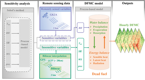
To address this challenge, this study sought to provide a practical approach to implementing the process-based model by reducing the number of meteorological variables required from satellites and employing high temporal-resolution geostationary satellite to generate required variables. Specifically, we employed sensitivity analysis for the process-based model to determine which variables are sensitive to DFMC. Then, the sensitive variables were derived from geostationary satellite with high resolution while other variables obtained from easily assessed meteorological gridded data, such as the Global Forecast System (GFS). Our overarching goal was to estimate large-scale gridded DFMC using a process-based model, which can ultimately contribute to fire attributes such as rate of spread, flame dimensions and fuel consumption.

2. Materials

2.1. Study area

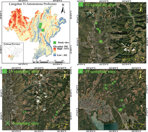
The Liangshan Yi Autonomous Prefecture (hereafter Liangshan) is situated in Sichuan Province, southwest China (102◦15′ E, 28◦15′ N), and was selected as the study area due to its heightened susceptibility to wildfires, which have escalated in frequency over the past decade (Quan, Li, et al. 2021). Encompassing an area of over 60,000 km², this region is experiencing notable shifts in fire regimes. This area is not only characterized by elevated fire activity but also comprises diverse climatological, topographic, and ecological regions (Zhang et al. 2020), rendering it suitable for establishing a robust DFMC monitoring methodology. Vegetation in this area includes closed evergreen broadleaf forests, open deciduous broadleaf forests, closed deciduous broadleaf forests, open evergreen needle-leaf forests, closed evergreen needle-leaf forests, and shrubs (Zhang et al. 2021). The region features a subtropical monsoon climate with an average annual temperature of 8.2°C and a rainfall of 990 mm (Y. Li et al. 2022). The study area features diverse terrain, with elevations ranging from 361 m to 5371 m. Elevation data obtained from the Advanced Spaceborne Thermal Emission and Reflection Radiometer (ASTER) Global Digital Elevation Model (GDEM) (Tachikawa et al. 2011) are depicted in Figure 1.

Figure 1. Location and sampling sites (96 study sites located in 3 areas) in Liangshan Yi Autonomous Prefecture. The background DEM map used in the upper left map is from ASTER GDEM 30M. The other three maps (1, 2, and 3) used World_Imager from the Environmental Systems Research Institute (ESRI) as the background map.

2.2. Data

2.2.1. Field-measured DFMC

If dead fuel (such as leaves, twigs, etc.) just after collection is weighted (wet mass) and dried in an oven (Dry mass), the DFMC can be calculated using Equation (1)(1) $\mathrm{DFMC}(\mathrm{\%})=\frac{\mathrm{Wet}\mathrm{mass}-\mathrm{Dry}\mathrm{mass}}{\mathrm{Dry}\mathrm{mass}}\times 100$(1) .

(1) $\mathrm{DFMC}(\mathrm{\%})=\frac{\mathrm{Wet}\mathrm{mass}-\mathrm{Dry}\mathrm{mass}}{\mathrm{Dry}\mathrm{mass}}\times 100$(1)

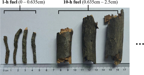
According to the equilibrium moisture time-lag theory (Fosberg and Deeming 1971; Nelson 1984), fuels dry in a negative exponential curve under constant temperature and humidity conditions. The time lag of 1-h is the time to achieve approximately 63% of the change from the initial DFMC to a steady moisture content named EMC (Catchpole et al. 2001). Fuels are categorized as 1-, 10-, 100- and 1000-h fuels, with each category associated with the diameter of fuel (Bradshaw et al. 1984). The 1-h fuels usually refer to those with diameter less than 0.635 cm (Figure 2). During the period from 5 December 2020, to 3 May 2021, we collected 1-h dead fuels at 96 sites in Liangshan (Figure 1). These sites were selected due to their relative homogeneity in terms of species composition, aspect, and slope both within and around each site. Considering the dominance of closed evergreen needle-leaf forests in Liangshan (Xie et al. 2022), our sampling efforts concentrated on collecting dead fuels beneath the canopy of Pinus yunnanensis. To ensure representative sampling, three plots were established at each site location. At least of 70 g of fuel was collected from each plot, resulting in a total sample weight exceeding 200 g for each site. To prevent any moisture loss, the collected samples were promptly sealed in pre-weighed plastic bags and transported to a field laboratory. The initial weight of each sample was determined by subtracting the weight of the plastic bag from the wet weight. The samples were then dried in an oven at 105°C for a minimum of 24 hours, followed by reweighing to ascertain their dry weight. To efficiently cover large areas, each site was sampled only once without any repeated collections.

Figure 2. Diagram of dead fuel. Where 1-h dead fuel usually refers to dead fuel with diameter less than 0.635 cm.

The site homogeneity was assessed using the coefficient of variation (CV, %) provided by Yebra et al. (2019). CV was calculated by dividing the standard deviation by NDVI_{mean,5kmmbuffer} of all the Landsat pixels within a 5 km × 5 km buffer that matched the Himawari-8 LST and SR pixel size (CV_Landsat, Equation (2)(2) $\frac{\mathrm{NDV}{\mathrm{I}}_{\mathit{Std},5\mathit{kmbuffer}}}{\mathrm{NDV}{\mathrm{I}}_{\mathit{mean},5\mathit{kmbuffer}}}\times 100\mathrm{\%}<\mathrm{CV}$(2) ).

(2) $\frac{\mathrm{NDV}{\mathrm{I}}_{\mathit{Std},5\mathit{kmbuffer}}}{\mathrm{NDV}{\mathrm{I}}_{\mathit{mean},5\mathit{kmbuffer}}}\times 100\mathrm{\%}<\mathrm{CV}$(2)

Where NDVI_{Std,5kmbuffer} and NDVI_{mean,5kmbuffer} represent the standard deviation and mean value NDVI of all the pixels from Landsat (Landsat 8 OLI) within the buffer corresponding to Himawari-8 LST pixel size, respectively. The CV value ranged from 5 (strict filtering) to 50 (no filtering). We used a CV value of 10 specifically for forest areas as recommend by Quan et al. (2021c) and 89 sites were homogeneous for our study.

2.2.2. Field-measured meteorological variables

Replacing a single remotely sensed variable with field measurement can determine the significant impact of that variable on DFMC estimation, as satellite-derived meteorological data are often less accurate than field measurements (Nolan, de Dios, et al. 2016). For example, if field-measured T_air is substituted for satellite-derived T_air without improving the accuracy of the estimated DFMC, this could confirm the limited contribution of T_air. Therefore, field measurements were conducted at each site where dead fuel samples were collected.

Brown et al. (2022)reported that SR has minimal impact on DFMC. Moreover, no rainfall occurred during the collection of dead fuel samples. Hence, we concentrated on field measurements of T_air, RH and WS at a height of 2 m using Testo 608-H2 and Digital Anemometer, respectively. Observed T_air ranged from 8.6°C to 37.3°C, and recorded RH varied between 8.96% and 79.17% across the field measurements. Measured WS values at various sites and on different days ranged from 0.2 to 2.7 m/s, with high WS values observed in valleys or on mountaintops).

2.2.3. Satellite data

The satellite data used in this study are presented in Table 1. Given that process-based models necessitate high temporal resolution meteorological data, we predominantly relied on Himawari-8 imagery, available at 10-minute intervals. Nieto et al. (2010) and Nolan et al. (2016b) employed LST, NDVI, SR, and water vapor (WV) to compute T_air and RH. We used the SR data from the product (5 km, 10 min) provided by Japan Aerospace Exploration Agency (JAXA). However, as JAXA does not provide LST products, we acquired the Himawari-8 LST product (5 km, hourly) from the Copernicus Global Land Service (CGLS), a component of Copernicus, Europe’s Earth Observation program. The CGLS focuses on monitoring vegetation, the water cycle, the energy budget, and the terrestrial cryosphere (Bayat et al. 2021; Freitas et al. 2013). The Himawari-8 LST product is derived from the top-of-atmosphere brightness temperatures of atmospheric window channels in the infrared range (Freitas et al. 2013). In addition, we used the Himawari-8 reflectance data, encompassing the near-infrared band (wavelength = 0.86 μm) and the red band (wavelength = 0.64 μm), to compute the NDVI. Since the spatial resolution of the reflectance data is 2 km, we resampled the computed NDVI to a resolution of 5 km using bilinear interpolation to align with the resolutions of LST and SR. Since Himawari-8 does not provide WV products, we used the WV product from Geo-KOMPSAT 2A (GK2A). Launched on 5 December 2018, the GK2A satellite provides a WV product (named Total Precipitable Water) with a resolution of 6 km every 10 minutes. We resampled the GK2A WV at the sampling time to 5 km using bilinear interpolation.

Table 1. The satellite data (including himawari-8 and GK2A) and gridded weather data (GFS) used in this study.

Sources	Datasets	Temporal ranges	Spatial resolution	Temporal resolution	Target variables
Himawari-8	JAXA Short Wave Radiation	2020.12.05–2021.05.03	5 km	10 minutes	SR
	CGLS Houly LST		5 km	1 hour	LST
	Himawari-8 reflectance		2 km	10 minutes	NDVI
GK2A	Total Precipitable Water		6 km	10minutes	WV
GFS	Wind speed		0.25°	1 hour	WS
	Precipitation		0.25°	1 hour	prec

2.2.4. Gridded weather data

We integrated GFS as supplementary data to enhance our analysis by accessing variables challenging to obtain from Himawari-8 or less sensitive to DFMC estimation. GFS has gained wide recognition in meteorological disaster predictions, including typhoon tracking and flood forecasting, due to its exceptional forecast accuracy (Hsiao et al. 2013; Lai and Peng 2022; Lu et al. 2016). The GFS is generated by the National Centers for Environmental Prediction (NCEP) and provides forecasts of various meteorological parameters for up to 384 hours. Initially, hourly forecasts are available for the first 120 hours, followed by updates every 3 hours up to 240 hours, and subsequently every 8 hours. For our study, we exclusively utilized the GFS data at hour 0, representing current conditions. Specifically, we extracted the required variables (such as WS and prec, Table 1) from the GFS dataset at the corresponding sampling time. To ensure compatibility with the resolution of Himawari-8 LST, we applied bilinear interpolation to interpolate the data from GFS into a 5 km grid.

3. Methods

Our modeling approach is specifically designed to monitor remotely sensed DFMC using a process-based model, Fuel Stick Moisture Model (FSMM, detailed in Section 3.1), and its known link to meteorological drivers, as shown in Figure 3. We conducted a sensitivity analysis for the FSMM to determine the most sensitive meteorological variables for estimating DFMC. Subsequently, we derived this sensitive variable using satellite data from Himawari-8 (explained in Section 3.3), while less sensitive variables were obtained directly from GFS. With the determined meteorological variables to operate FSMM, we estimated and validated the DFMC of Liangshan at 89 sites. Additionally, an EMC model and random forest regression (explained in Section 3.4) were also used for comparison. We evaluated the remotely sensed DFMC using the determination coefficient (R²), the root mean square error (RMSE), and the mean absolute error (MAE).

Figure 3. The flow chart of our approach, including sensitivity analysis, remote sensing of meteorological variables and process-based models.

3.1. Fuel stick moisture model (FSMM)

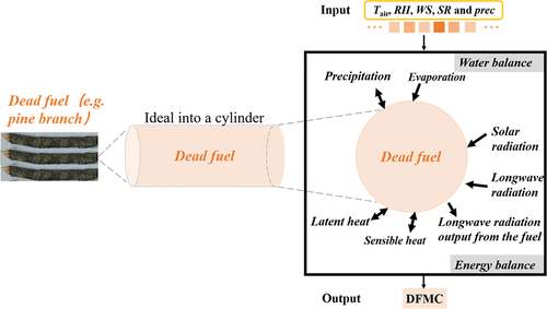
To compute DFMC from meteorological variables, we applied the FSMM, a process-based model renowned for its adeptness in simulating water and energy balance, as demonstrated in previous studies (Van der Kamp, Moore, and Mckendry 2017). As depicted in Figure 4, the FSMM encompasses various physical processes affecting DFMC changes, including evaporation, precipitation absorption, latent heat flux, etc. With hourly T_air, RH, WS, SR, and prec data, the FSMM can provide hourly DFMC estimates for various fuel types such as 1-, 10-, 100-, and 1000-h (Fan and He 2021). The parameterization scheme adopted for the FSMM in this study was based on the scheme utilized in a localization test conducted in Liangshan by Fan et al. (2023).

Figure 4. The schematic diagram of the process-based model, FSMM, in which the dead fuel (e.g. pine branches) is idealized as a cylinder. The FSMM modelled the water and energy balance processes with input of meteorological variables.

3.2. Sensitivity analysis for FSMM

Sobol’s method was selected for sensitivity analysis because it is global and independent of non-monotonic models (Nossent, Elsen, and Bauwens 2011). The FSMM model can be simplified to a function:

(3) $\mathit{y}=\mathit{F}\left(\mathit{x},\mathit{\theta }\right)=\mathit{F}\left(T_{\mathit{air}},\mathit{RH},\mathit{SR},\mathit{WS},\mathit{prec}\right)$(3)

Where the F(x, $\mathit{\theta }$) is the FSMM that contains energy and water balance equations. And y is the FSMM model outputs, x is the input meteorological variables, $\mathit{\theta }$ is the parameter set. Sobol’s method assesses the sensitivity of parameters by determining the variance of y with changes in input variables$\mathit{x}$. As shown in Sobol (1993), the total variance of y was decomposed into some component variances generated from individual variables (T_air, RH, SR, WS, prec) and variable interactions (T_air&RH, T_air&SR, T_air&RH&SR, etc.):

(4) $\mathit{V}\left(\mathit{y}\right)=\sum _i{V}_i+\sum _{\mathit{i}<\mathit{j}}{V}_{\mathit{ij}}+\sum _{\mathit{i}<\mathit{j}<\mathit{k}}{V}_{\mathit{ijk}}+\cdots +V_{1,2,\cdots ,\mathit{m}}$(4)

Where V_i is the variance of i_th component of input variables, denoted as x. V_ij is the portion of model output variance because of the interaction of variables x_i and x_j. The variable m is the total number of inputs. The sensitivity of single variables (V_i) or variable interactions (V_ij, V_ijk …) was assessed according to their proportion contributions to the total variance (V). Sobol’s sensitivity indices were calculated as:

(5) $\mathrm{First}\mathrm{order}{S}_i=\frac{V_i}{\mathit{V}}$(5)

(6) $\mathrm{Totalorder}{S}_{\mathit{Ti}}=1-\frac{{\mathit{V}}_{\sim \mathit{i}}}{\mathit{V}}$(6)

Where first-order sensitivity index (S_i) represents the sensitivity of a single variable x_i; V_~i is the average variance related to all variables except for x_i. For x_i, the total order sensitivity (S_Ti) includes its independent and interactive effects up to all other variables. If x_i has a large S_i and a small S_Ti, it only influences the model performance by individual variables. As Tang et al. (2007) described, variables contributing less than 1% on average to the total order sensitivity were classified as insensitive.

Determining the range of each variable is essential for sensitivity analysis. As shown in Table 2, the value intervals of input variables were determined based on the weather conditions of Liangshan. According to data from China Meteorological Data Service Center (CMDSC), the T_air ranged from −10°C to 40°C, and the SR did not exceed 1500 W·m⁻² in Liangshan. Since hurricane (>32.6 m·s⁻¹) and storm (>15.9 mm·hour⁻¹) were rare in Liangshan, the WS was capped at no more than 32.6 m·s⁻¹ and the prec at no more than 15.9 mm·hour⁻¹. For a balance between computing cost and reliable analysis, a sample size of 500 was used, resulting in 3500 model evaluations to calculate S_i and S_Ti. The detailed steps are as follows:

1. Define input parameter ranges: Determine the range of input parameters (T_air, RH, SR, WS, prec) to be analyzed (refer to Table 2).

2. Sample input parameters: Use Monte Carlo Sampling to generate a set of random samples (500 in this study) within the specified parameter ranges.

3. Run the model: For each combination of parameter samples, execute the model using the sampled values of the input parameters and record the corresponding output results. Equation (3)(3) $\mathit{y}=\mathit{F}\left(\mathit{x},\mathit{\theta }\right)=\mathit{F}\left(T_{\mathit{air}},\mathit{RH},\mathit{SR},\mathit{WS},\mathit{prec}\right)$(3) was used in this step.

4. Calculate First-order Sensitivity Index: Compute the first-order sensitivity index to assess the contribution of individual parameters to the output (using Equations (4)(4) $\mathit{V}\left(\mathit{y}\right)=\sum _i{V}_i+\sum _{\mathit{i}<\mathit{j}}{V}_{\mathit{ij}}+\sum _{\mathit{i}<\mathit{j}<\mathit{k}}{V}_{\mathit{ijk}}+\cdots +V_{1,2,\cdots ,\mathit{m}}$(4) and (5(5) $\mathrm{First}\mathrm{order}{S}_i=\frac{V_i}{\mathit{V}}$(5) )). This entails evaluating the model for various values of each parameter independently.

5. Calculate Total Sensitivity Index: Determine the total sensitivity index to account for interactions between parameters and their combined effects on the output (using Equations (4)(4) $\mathit{V}\left(\mathit{y}\right)=\sum _i{V}_i+\sum _{\mathit{i}<\mathit{j}}{V}_{\mathit{ij}}+\sum _{\mathit{i}<\mathit{j}<\mathit{k}}{V}_{\mathit{ijk}}+\cdots +V_{1,2,\cdots ,\mathit{m}}$(4) and (6(6) $\mathrm{Totalorder}{S}_{\mathit{Ti}}=1-\frac{{\mathit{V}}_{\sim \mathit{i}}}{\mathit{V}}$(6) )). This step involves investigating the joint effects of parameter pairs (e.g. T_air&RH), triplets (e.g. T_air&RH&SR), and so on.

6. Interpret the results: Analyze the calculated First-order Sensitivity Index and Total Sensitivity Index to comprehend the sensitivity of the output to the input parameters. Identify the parameters with the greatest influence on the output and evaluate the importance of their interactions.

Table 2. Ranges of input meteorological variables used for sensitivity analysis (in simulations). These ranges were determined using the prior knowledge of meteorological conditions in Liangshan.

Variables	Tair (℃)	RH (%)	SR (W·m^−2)	WS (m·s^−1)	prec (mm·hour^−1)
Ranges	(−10, 40)	(0, 100)	(0, 1500)	(0, 32.6)	(0, 15.9)

3.3. Remote sensing of meteorological variables

Table 3 shows the summary of methods used to estimate meteorological variables. Among five variables (T_air, RH, WS, SR, and prec) required for the FSMM, SR can be easily obtained from Himawari-8 product, but there is no feasible approach to calculate WS and prec from Himawari-8. Thus, our focus was on acquiring T_air and RH from Himawari-8, given the absence of T_air and RH products from the Himawari-8 satellite.

Table 3. Summary of methods used to estimate meteorological variables. Among them, T_air, RH and SR were from satellites while WS and prec from GFS.

Variable	Abbreviation	Approach
Air temperature	Tair	Calculated from LST, NDVI and SR
Relative humidity	RH	Calculated from Tair and WV
Solar radiation	SR	Himawari-8 product
Wind speed	WS	From GFS (no feasible approach from Himawari-8)
Precipitation	prec	From GFS (no feasible approach from Himawari-8)

Based on the methods used in Nolan et al. (2016b) and Nieto et al. (2010), RH can be calculated from remotely sensed T_air and WV using Equation (7(7) $\mathit{RH}=\frac{{\mathit{e}}_{\mathrm{a}}}{e_{\mathrm{s}}}\cdot 100\mathrm{\%}$(7) -9(9) $e_{\mathrm{a}}=\frac{\mathit{g}\cdot \mathit{WV}\cdot \left(\mathit{\lambda }+1\right)}{\delta }$(9) ).

(7) $\mathit{RH}=\frac{{\mathit{e}}_{\mathrm{a}}}{e_{\mathrm{s}}}\cdot 100\mathrm{\%}$(7)

(8) $e_{\mathrm{s}}=0.6108\cdot exp\left(17.27\cdot \frac{{\mathit{T}}_{\mathrm{air}}}{T_{\mathrm{air}}+237.3}\right)$(8)

(9) $e_{\mathrm{a}}=\frac{\mathit{g}\cdot \mathit{WV}\cdot \left(\mathit{\lambda }+1\right)}{\delta }$(9)

Where $e_{\mathrm{a}}$ represents the water vapor pressure and $e_{\mathrm{s}}$ denotes the saturation vapor pressure. The symbol g stands for the acceleration due to gravity (9.8 m·s⁻²). The parameter $\mathit{\delta }$ represents the ratio of the specific gas constants of water vapor and dry air (0.622). WV can be obtained from GK2A. The symbol λ denotes the exponent of the power law describing the moisture decrease with altitude through the atmospheric profile. The value of λ varies with latitude and season, and was calculated following Smith (1966) for the northern hemisphere areas.

It is noted from Equation (8)(8) $e_{\mathrm{s}}=0.6108\cdot exp\left(17.27\cdot \frac{{\mathit{T}}_{\mathrm{air}}}{T_{\mathrm{air}}+237.3}\right)$(8) that T_air is necessary to compute $e_{\mathrm{s}}$. Remotely sensed T_air is commonly determined using the Temperature-Vegetation Index (TVX) method (Nieto et al. 2010; Nolan, de Dios, et al. 2016), which postulates that LST over a fully vegetated canopy correlates with T_air. Consequently, a linear relationship between LST and NDVI can be defined within a designated X by X pixel window (where X can denote values such as 1, 3, 5, 7, etc.) (Nolan, de Dios, et al. 2016). T_air is subsequently estimated by extrapolating this correlation to a fully vegetated canopy (NDVI_max) (Nieto et al. 2011; Stisen et al. 2007). The NDVI_max for various types of forests is documented in Nieto et al. (2010). The fundamental assumption underlying the TVX method is the presumed negative correlation between LST and NDVI (Stisen et al. 2007). However, our experimental findings in Liangshan, characterized by complex topographical features, suggested that the expected negative correlation between LST and NDVI was not consistently observed. Consequently, the TVX method cannot be utilized to estimate T_air as previously suggested by Nolan et al. (2016b) and Nieto et al. (2010).

Therefore, to address the limitations of the TVX method, alternative approaches for remotely sensed T_air are necessary. Previous studies have introduced a energy balance method for T_air estimation using Equation (10)(10) $T_{\mathrm{air}}=\mathit{LST}-\frac{\mathit{Brc}}{1+\mathit{Brc}}\cdot \frac{\left(1-\mathit{\epsilon }\right)\cdot {\mathit{R}}_{\mathrm{n}}\cdot r_{\mathrm{a}}}{\mathit{\rho }\cdot C_{\mathrm{p}}}$(10) (Hou et al. 2013).

(10) $T_{\mathrm{air}}=\mathit{LST}-\frac{\mathit{Brc}}{1+\mathit{Brc}}\cdot \frac{\left(1-\mathit{\epsilon }\right)\cdot {\mathit{R}}_{\mathrm{n}}\cdot r_{\mathrm{a}}}{\mathit{\rho }\cdot C_{\mathrm{p}}}$(10)

Where $\mathit{\rho }$ is the air density (1.293 kg·m⁻³), $C_{\mathrm{p}}$ is the air-specific heat at constant pressure (1.006 × 10³ J·kg⁻¹·°C⁻¹)).$R_{\mathrm{n}}$ is net radiation (Equation (11)(11) $R_{\mathrm{n}}=\left(1-\mathit{\alpha }\right)\times \mathit{SR}+L_{\mathrm{n}}$(11) ). Brc is the Bowen ratio coefficient (see Equation (13)(13) $\mathit{Brc}=\frac{{\mathit{T}}_{\mathrm{su}}\left(\mathrm{NDVI}\right)-\mathit{LST}}{T_{\mathrm{su}}\left(\mathrm{NDVI}\right)-T_{\mathrm{sl}}\left(\mathrm{NDVI}\right)}-1$(13) ). $r_{\mathrm{a}}$ is the aerodynamic resistance (see Equation (17)(17) $r_{\mathrm{a}}=\frac{250}{1+0.54\cdot {\mathit{W}}_{\mathrm{s}}}$(17) ). $\mathit{\epsilon }$ is land surface emissivity (see Equation (18)(18) $\mathit{\epsilon }=\left\{\begin{array}{cc}{\epsilon }_{\mathit{soil}}& \mathit{NDVI}<0.2\\ {\epsilon }_v& \mathit{NDVI}>0.5\\ {\epsilon }_v\cdot P_v+{\epsilon }_{\mathit{soil}}\cdot \left(1-P_v\right)& 0.2\le \mathit{NDVI}\le 0.5\end{array}\right.$(18) ).

$R_{\mathrm{n}}$ can be calculated according to Davies (1967).

(11) $R_{\mathrm{n}}=\left(1-\mathit{\alpha }\right)\times \mathit{SR}+L_{\mathrm{n}}$(11)

(12) $L_{\mathrm{n}}=\in \cdot \mathit{\sigma }\cdot \mathit{LS}{T}^4\cdot \left(0.39-0.05\cdot {{\mathit{e}}_{\mathrm{a}}}^{1/2}\right)$(12)

Where $\mathit{\sigma }$ is the Stefan-Bolzmann constant (5.6697 × 10⁻⁸ W·m⁻²·K⁻⁴) and $\in$ is the water emissivity (0.98).

The simple estimation model for Brc is proposed by Su et al. (2001).

(13) $\mathit{Brc}=\frac{{\mathit{T}}_{\mathrm{su}}\left(\mathrm{NDVI}\right)-\mathit{LST}}{T_{\mathrm{su}}\left(\mathrm{NDVI}\right)-T_{\mathrm{sl}}\left(\mathrm{NDVI}\right)}-1$(13)

(14) $T_{\mathrm{su}}(\mathrm{NDVI})=a_{\mathrm{u}}+b_{\mathrm{u}}\cdot \mathrm{NDVI}$(14)

(15) $T_{\mathrm{sl}}(\mathrm{NDVI})=a_{\mathrm{l}}+b_{\mathrm{l}}\cdot \mathrm{NDVI}$(15)

(16) $\mathrm{NDVI}=\frac{\mathit{Re}{\mathit{f}}_{\mathrm{nir}}-\mathit{Re}{f}_{\mathrm{red}}}{\mathit{Re}{f}_{\mathrm{nir}}+\mathit{Re}{f}_{\mathrm{red}}}$(16)

According to Hou et al. (2013), $a_{\mathrm{u}}$, $b_{\mathrm{u}}$, $a_{\mathrm{l}}$, and $b_{\mathrm{l}}$ were estimated as − 18.283, 47.834, −9.154, and 34.395, respectively. NDVI can be calculated using Himawari-8 reflectance. Ref_nir and Ref_red represent the reflectance of the near-infrared (wavelength = 0.86 $\mathit{\mu }\mathrm{m}$) and red (wavelength = 0.64 $\mathit{\mu }\mathrm{m}$) bands, respectively.

The $r_{\mathrm{a}}$ is the aerodynamic resistance, which can be calculated according to Thom and Oliver (1977).

(17) $r_{\mathrm{a}}=\frac{250}{1+0.54\cdot {\mathit{W}}_{\mathrm{s}}}$(17)

The land surface emissivity ($\mathit{\epsilon }$) can be expressed according to Sobrino et al. (1996).

(18) $\mathit{\epsilon }=\left\{\begin{array}{cc}{\epsilon }_{\mathit{soil}}& \mathit{NDVI}<0.2\\ {\epsilon }_v& \mathit{NDVI}>0.5\\ {\epsilon }_v\cdot P_v+{\epsilon }_{\mathit{soil}}\cdot \left(1-P_v\right)& 0.2\le \mathit{NDVI}\le 0.5\end{array}\right.$(18)

Where ${\epsilon }_{\mathrm{soil}}$ and ${\epsilon }_{\mathrm{v}}$ are the emissivity of soil, and vegetation, respectively, and are set as 0.972, and 0.995 based on Hou et al. (2013). $P_{\mathrm{v}}$ is the fraction of vegetation cover estimated by Carlson and Ripley (1997).

3.4. Model comparison

3.4.1. The Simard

EMC models such as the Simard only require T_air (℃) and RH for DFMC estimation. The expression of the Simard EMC method came from regression analysis of data pertaining to the EMC of wood (Simard 1968), see Equation (19)(19) $\mathit{EM}{C}_{\mathit{simard}}=\left\{\begin{array}{cc}0.03+0.2626\mathit{RH}-0.00104\mathit{RH}\cdot T_{\mathit{air}}& \mathit{RH}<10\\ 1.76+0.1601\mathit{RH}-0.0266T_{\mathit{air}}& 10\le \mathit{RH}<50\\ 21.06-0.4944\mathit{RH}+0.005565\mathit{R}{H}^2-0.00063\mathit{RH}\cdot T_{\mathit{air}}& \mathit{RH}\ge 50\end{array}\right.$(19) .

(19) $\mathit{EM}{C}_{\mathit{simard}}=\left\{\begin{array}{cc}0.03+0.2626\mathit{RH}-0.00104\mathit{RH}\cdot T_{\mathit{air}}& \mathit{RH}<10\\ 1.76+0.1601\mathit{RH}-0.0266T_{\mathit{air}}& 10\le \mathit{RH}<50\\ 21.06-0.4944\mathit{RH}+0.005565\mathit{R}{H}^2-0.00063\mathit{RH}\cdot T_{\mathit{air}}& \mathit{RH}\ge 50\end{array}\right.$(19)

The 1-h can be then calculated following Fosberg and Deeming (1971), see Equation (20)(20) $\mathit{DFM}{C}_{1-\mathit{h}}=1.03\times \mathit{EMC}$(20) .

(20) $\mathit{DFM}{C}_{1-\mathit{h}}=1.03\times \mathit{EMC}$(20)

3.4.2. Random forest regression

Random forest regression was selected due to its demonstrated utility in estimating DFMC in South Korea (H. Lee et al. 2020). As a machine-learning method based on the regression tree algorithm (Breiman 2001), random forest regression finds widespread application in wildfire risk assessment (Quan, Xie, et al. 2021; Wang et al. 2023). This entails creating an ensemble of multiple regression trees using a bootstrapped training dataset (H. Lee et al. 2020). Each tree in the random forest is trained on a subset of the available variables. The final regression result derives from aggregating the votes of these multiple trees (James et al. 2013). A reduction in the correlation between decision trees within the random forest corresponds to an improvement in the reliability of the ensemble (Stewart J Richard 1996). Advantages of random forest regression encompass: (i) facile predictor inclusion or exclusion contingent on data availability and user demands, (ii) integration of both continuous and categorical predictors, (iii) automatic computation of variable importance scores to evaluate individual predictors’ contribution to the final model, (iv) necessitating only a small number of user-specified model parameters, and (v) mitigating overfitting risk (Hutengs and Vohland 2016). In this study, random forest regression was employed to estimate the DFMC using meteorological variables including T_air, RH, SR, WS, and prec. The RandomForestRegressor package (Geurts, Ernst, and Wehenkel 2006) in Python was employed for implementing the random forest regression model. The number of trees in the random forest was set to 100 to balance computational cost with reliable performance. Each tree in random forest regression method used a minimum node size of 5 as the default value. Ten-fold cross-validation was employed to validate the performance of random forest.

4. Results

4.1. Results of sensitivity analysis of the process-based model

The sensitivity analysis results (S_i, S_Ti) of the process-based model output to meteorological variables are presented in Table 4. It is observed that DFMC is not significantly influenced by SR, as evidenced by its S_Ti value being less than 0.01. While other variables have S_Ti values greater than 0.01, their sensitivities exhibit considerable variations. The S_i value of prec is less than 0.01 while the S_Ti is 0.04, indicating that the independent effect of prec on DFMC is negligible and its interactive effects up to all other variables have a slight influence on DFMC. Although T_air and WS have non-negligible independent and interactive influences on DFMC (S_i >0.01 and S_Ti >0.01), their influences are much smaller than RH (S_i of 0.75, and S_Ti of 0.80). These findings emphasize that RH plays a dominant role in determining DFMC compared to the other meteorological variables analyzed.

Table 4. The S_i, S_Ti of meteorological variables (including T_air, RH, SR, WS and prec) required by the process-based model, FSMM.

Sensitivity	Tair	RH	SR	WS	prec
Si	0.06	0.75	<0.01	0.09	<0.01
STi	0.10	0.80	<0.01	0.15	0.04

4.2. Evaluate the performance of DFMC

According to the sensitivity analysis results in Section 4.1, RH exhibits a much higher sensitivity compared to other variables. Therefore, for the application of the process-based model, FSMM, we adopted an approach using satellite-derived RH and other variables obtained from easily assessed GFS data. The DFMC estimation results from this approach are shown in Figure 5(b). For comparison, the performances of the FSMM using other approaches are also presented: all variables from GFS (Figure 5(a)), satellite-derived RH, T_air and other variables from GFS (Figure 5(c)), satellite-derived RH with field-measured T_air and WS (Figure 5(d)), and field-measured RH, T_air and WS (Figure 5(e)). It is worth mentioning that the SR data used in all approaches were obtained from the Himawari-8 product, as it can be obtained directly and easily (not repeated hereafter).

Figure 5. Performance of FSMM using different sources of input variables: (a) All input variables from GFS, (b) Satellite-derived RH and other variables from GFS, (c) Satellite-derived RH, T_air, SR, and other variables from GFS, (d) Satellite-derived RH and field-measured T_air and WS. (e) Field-measured RH, T_air and WS.

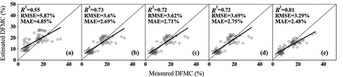
Using only the variables from GFS resulted in the poorest DFMC estimates with highest RMSE (5.87%) and MAE (4.85%), characterized by noticeable overestimations and underestimations (Figure 5(a)). This suggests that relying solely on GFS data is insufficient for accurate DFMC estimation. However, with the introduction of satellite-derived RH along with the other variables from GFS (Figure 5(b)), the accuracy of DFMC estimation by FSMM significantly improved (R² increased from 0.55 to 0.73, and RMSE decreased from 5.87% to 3.60%). This highlights the critical role of RH in DFMC estimation, which is consistent with the conclusion in Section 4.1. In contrast, when satellite-derived RH, T_air, SR were used, the accuracy of DFMC did not improve (Figure 5(c)). Even when field-measured T_air and WS were used to replace the GFS T_air and WS data, there was no significant improvement in the performance of the FSMM (Figure 5(d)). This finding further supports the conclusion stated in Section 4.1 that T_air and WS have minimal influence on the estimation of DFMC. However, when satellite-derived RH was replaced with field-measured RH, the estimated DFMC exhibited higher precision (Figure 5(e)). This once again confirms the importance of RH in accurately estimating the DFMC.

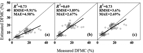
In practical applications, relying solely on measured meteorological variables to monitor DFMC at large scales is not feasible. Therefore, we emphasized the approach using satellite-derived RH and other variables from the GFS, as it successfully employed the FSMM to estimate accurate remotely sensed DFMC. Through this approach, we compared the performance of FSMM with that of an EMC model (the Simard), and random forest regression (see Figure 6). The random forest regression exhibited both underestimation and overestimation to some extent. The Simard model exhibited significant underestimation of the DFMC. In contrast, the FSMM model showed the best performance, achieving the highest R² value (0.73) and the lowest RMSE (3.60%).

Figure 6. The performance of the Simard (a), Random forest regression (b), and the FSMM (c) Using satellite-derived RH and other variables from GFS.

4.3. DFMC dynamics before wildfires

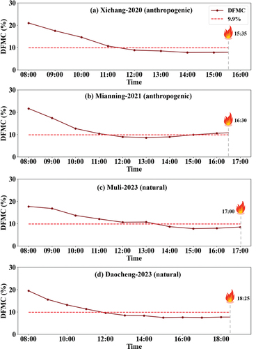
Employing the process-based model FSMM with satellite-derived RH and other variables from GFS resulted in accurate DFMC (Section 4.2). Consequently, we applied this approach to map the 1-h DFMC in Liangshan from 8:00 to 15:00 on 30 March 2020 (local time, UTC + 8), immediately preceding a fire occurrence at 15:35 (Figure 7). The results clearly depict a continuous decline in DFMC in Liangshan throughout the designated time period. Higher DFMC values were observed in the northeast region compared to the lower values in the west. Subsequently, we monitored the fluctuations in DFMC within the burned area preceding the wildfires (Xichang-2020, Mianning-2021, Muli-2023, and Daocheng-2023) by averaging the DFMC values of corresponding pixels. Xichang-2020, Mianning-2021 were anthropogenic fires caused by human activities, while the other two are natural fries ignited by lightning. As shown in Figure 8(a), the 1-h DFMC preceding the Xichang-2020 fire decreased from 21% to 7.81% between 8:00 and 15:00. After 12:00, the DFMC fell below the fire potential threshold (9.9%, as suggested by Nolan et al. (2016a)). The other natural fire (Daocheng 2023) also occurred with DFMC below the threshold at the time of ignition. Conversely, another anthropogenic fire (Mianning-2021) was ignited by a discarded cigarette butt and occurred when the DFMC was above the threshold.

Figure 7. The 1-h DFMC maps (hourly from local time 8:00 to 15:00) of Liangshan prior to the Xichang fire, which occurred at 15:35 on March 30, 2020. Maps with DFMC estimation were masked by evergreen needle-leaved forests in the global land-cover product (GLC_FCS30) (Zhang et al. 2021). The DFMC in the grey pixel is missing due to the lack of RH values caused by cloud cover. And the white pixel means that the vegetation type is not evergreen needle-leaved forests.

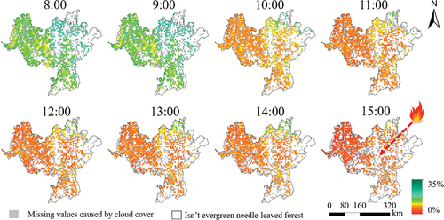
Figure 8. The DFMC trends in the burned area of wildfires ((a) Xichang-2020, (b) Mianning-2021, (c) Muli-2023, and (d) Daocheng-2023). The dashed red line indicates the threshold values (9.9%, as suggested by Nolan et al. (2016a)) associated with the fire potential in forests.

5. Discussion

5.1. The sensitivity of meteorological variables

The sensitivity analysis results in Section 4.1 indicate that DFMC is minimally affected by SR, as demonstrated by its S_Ti value being less than 0.01. Variations in SR primarily result in changes in T_air, while T_air directly affects evaporation, whereas SR does not play a direct role. Additionally, the S_i value of prec is less than 0.01, indicating the negligible independent effect of prec on DFMC. This could be attributed to the thin diameter (less than 0.635 cm) of the 1-h dead fuel, which may retain small amount of water and facilitate frequent vapor exchange (Matthews 2014). However, the S_Ti of prec is 0.04, exceeding the threshold of 0.01. This indicates that the interactive effects of prec with all other variables have a slight influence on DFMC. This may be associated with the tendency for rainfall to coincide with rising RH. Furthermore, WS has a relatively small S_i (0.09), but a larger S_Ti (0.15), indicating that the interactive effects of WS with all other variables are more significant than its independent effect. This finding is consistent with conclusions in previous literature, suggesting that DFMC is not sensitive to WS below the fiber saturation point (30%), especially in the absence of precipitation, when water content exchange resistance is primarily governed by sorption processes that are relatively unaffected by WS (Van der Kamp, Moore, and Mckendry 2017). Similar results can be observed for T_air, where fluctuations in T_air can cause slight adjustments in RH, ultimately contributing to evaporation. This explains why the interactive effects of T_air with all other variables exhibit higher magnitudes compared to its independent effect. In contrast, RH showed a significantly higher sensitivity in terms of both its independent effect (S_i = 0.75) and interactive effects (S_Ti = 0.80) compared to other variables. These findings are further supported by the results presented in Section 4.2.

Nevertheless, this sensitivity analysis result pertains specifically to 1-h DFMC. Finer fuel are less capable of retaining prec (Brown et al. 2022; Simard 1968). The 1-h dead fuel tends to rapidly evaporate stored water with changes in meteorological factors such as T_air and RH. Our study employed 1-h dead fuel as a case study to investigate the application process-based models. However, this relationship may vary for 10-h, 100-h, 1000-h fuels, as they possess greater water holding capacity. Nevertheless, this relationship can also be investigated using the method proposed in this study.

5.2. Performance of the process-based model

This study used a process-based model, FSMM, to monitor DFMC at regional scales through remote sensing. Our findings indicate that using satellite-derived RH and other variables from GFS, the FSMM still outperformed an EMC model (Simard), and an empirical method (random forest regression). This outcome aligns with the findings of Fan et al. (2023), who employed station meteorological data. This consistency suggests that the alteration of input data did not affect the performance comparison results between these models. EMC models such as the Simard model were developed based on historical experimental data and represent the wetting and drying regimes of the DFMC. However, these types of DFMC models were specifically designed for regions such as the United States and Canada, and may not be universally applicable to other regions, such as our study area, Liangshan, characterized by more complex terrain. Similarly, random forest regression heavily relied on field-measured DFMC to train the model, and lacks a direct representation of the physical processes such as heat and water vapor exchange (Matthews 2006). In contrast, process-based models such as FSMM incorporate complex physical processes, including water and energy balance equations, thereby enhancing their robustness in estimating DFMC.

5.3. Application of the process-based DFMC monitoring

The process-based model, FSMM, requires several variables (T_air, RH, WS, SR, and prec) to operate. However, obtaining all the variables from satellites remains challenging and time-consuming. Our results indicate that the performance of FSMM is heavily affected by RH while other variables have minimal influence. Our process-based DFMC monitoring approach, using satellite-derived RH and other variables from GFS, accurately estimated DFMC, while more accurate T_air and WS did not result in more accurate DFMC. This suggested that it may be not necessary to invest significant effort into obtaining all variables from satellites; instead, greater attention should be given to obtaining accurate remotely sensed RH. Previous studies have proposed effective methods for deriving RH using indicators including LST, NDVI, and WV from remote sensing data (Nieto et al. 2010; Nolan, de Dios, et al. 2016). Satellite products, including those from MODIS, Himawari-8, and GK2A, which provide LST, NDVI, and WV, such as facilitate the application of our approach (Freitas et al. 2013; Frouin and Murakami 2007; K.-S. Lee et al. 2020; Prince et al. 1998; Wan and Dozier 1996). However, it is important to note that optical satellites are often affected by cloud cover. As shown in Figure 7, our DFMC maps exhibit many missing values (gray pixels) in Liangshan due to cloud cover. This can be attributed to the absence of the meteorological variables that are necessary for the process-based model in those specific pixels. During the estimation of DFMC, all of the drivers except for RH were derived from GFS and were not influenced by clouds. The only driver can be affected by cloud cover is the remotely sensed RH from satellite. Therefore, future work should focus on addressing this issue, such as by utilizing spatiotemporal features (Y. Li et al. 2022).

DFMC is crucial for fire risk assessment and fire behavior simulation as it fundamentally influences fire occurrence, spread, and intensity (Rothermel 1983). Previous studies mainly focused on DFMC model development and paid little attention to large-scale DFMC estimating, which hinders the research on the contribution of DFMC to regional or global fire events. This study provided a practical approach to easily estimate large-scale DFMC and track DFMC dynamics before four wildfires (natural and anthropogenic). Our results showed that the DFMC before natural fires continuously decreased below the thresholds associated with the fire potential in forests until the fire outbreak. While DFMC values before the anthropogenic fires does not seem to be as low as those before the natural fires (Figure 8). One possible reason is that the complex impact of human activities on the environment may lead to fire occurrences that do not necessitate low DFMC as natural fire. However, drawing firm conclusions from just a few fires is difficult. To better understand these specific relationships, it is critical to make a concerted effort to track DFMC changes before thousands of fires, which may yield some interesting findings in future research. The threshold (9.9%) was determined by Nolan et al. (2016a) using daily DFMC, which may be not appropriate to represent hour-by-hour changes in the DFMC. Our study provides a more accurate characterization of pre-fire DFMC using hourly observations. In addition, the threshold was determined based on fire events in Australia, while our study area is located in southwestern China. Therefore, further research is needed to determine a threshold that accurately represents conditions in southwest China. Our work can serve as a preliminary exploration of the relationship between DFMC and wildfires. However, further investigation is necessary to establish a quantitative relationship between DFMC and the occurrence, development, and burning intensity of fires. Additionally, mapping DFMC in different terrains and climate zones worldwide, understanding whether the thresholds associated with fire potential are consistent across regions, and characterizing the relationship between DFMC and fires in diverse geographic areas are important and unresolved questions. Addressing these questions will contribute to improved global fire risk assessment and enable more effective fire hazard warnings.

6. Conclusion

In summary, our study presents an effective approach for estimating remotely sensed DFMC using a process-based model. Through sensitivity analysis on the process-based model, we found that RH is the most sensitive variable with a much higher sensitivity index compared to other variables. Therefore, we applied the process-based DFMC estimation process by using satellite-derived RH and other variables from the GFS. This approach not only addressed the challenge of obtaining multiple meteorological variables from satellites, but also provided accurate estimates of DFMC (R² = 0.73, RMSE = 3.60%, MAE = 2.69%). Compared to other commonly used models such as Simard, and random forest regression, the process-based model, FSMM, demonstrated superior performance. By employing our approach to track DFMC dynamics before the wildfire outbreak, we observed continuous decreasing trends. This highlights the applicability of our approach in supporting wildfire risk assessment and fire behavior prediction.

Acknowledgments

We are indebted to Xingwen Quan, Yiru Zhang, Zhanmang Liao, Yanxi Li, Tengfei Xiao, Gangqiang An, Gengke Lai and Lin Chen for field measurements and invaluable comments in the early stages of this study. This work was supported by the National Key R&D Program of China (Contract No. 2022YFC3003001) and the Sichuan Science and Technology Program (Contract No. 2023YFS0432).

Disclosure statement

No potential conflict of interest was reported by the author(s).

Data availability statement

The Himawari-8 LST data are available from Copernicus Global Land Service (CGLS) (https://land.copernicus.eu/global/products/lst, last visit on 12th September, 2023). The Himawari-8 SR and reflectance Data can be download using ftp (ftp.ptree.jaxa.jp, last visit on 12th September, 2023).The GK2A WV product (Total Precipitable Water) is available from National Meteorological Satellite Center (NMSC) of Korea Meteorological Administration (KMA) (https://datasvc.nmsc.kma.go.kr/datasvc/html/data/listData.do, last visit on 24th December, 2023). The 1-h field measured DFMC data used in this study will be made available on request.

Additional information

Funding

This work was supported by the National Key R&D Program of China (Contract No. 2022YFC3003001) and the Sichuan Science and Technology Program (Contract No. 2023YFS0432).

References

- Alves, M., A. Batista, R. Soares, M. Ottaviano, and M. Marchetti. 2009. “Fuel moisture sampling and modeling in Pinus elliottii Engelm. plantations based on weather conditions in Paraná-Brazil.” iForest-Biogeosciences and Forestry 2 (3): 99. https://doi.org/10.3832/ifor0489-002.
- Bayat, B., F. Camacho, J. Nickeson, M. Cosh, J. Bolten, H. Vereecken, and C. Montzka. 2021. “Toward Operational Validation Systems for Global Satellite-Based Terrestrial Essential Climate Variables.” International Journal of Applied Earth Observation and Geoinformation 95:102240. https://doi.org/10.1016/j.jag.2020.102240.
- Bilgic, H. H., and İ. Mert. 2021. “Comparison of Different Techniques for Estimation of Incoming Longwave Radiation.” International Journal of Environmental Science and Technology 18:601–18. https://doi.org/10.1007/s13762-020-02923-6.
- Boerner, R. E., J. Huang, and S. C. Hart. 2009. “Impacts of Fire and Fire Surrogate Treatments on Forest Soil Properties: A Meta‐Analytical Approach.” Ecological Applications 19 (2): 338–358. https://doi.org/10.1890/07-1767.1.
- Bowman, D. M., J. K. Balch, P. Artaxo, W. J. Bond, J. M. Carlson, M. A. Cochrane, C. M. D’Antonio, R. S. DeFries, J. C. Doyle, and S. P. Harrison. 2009. “Fire in the Earth System.” Science 324 (5926): 481–484. https://doi.org/10.1007/978-90-481-8716-4_3.
- Bradshaw, L. S., J. E. Deeming, R. E. Burgan, and J. D. Cohen. 1984. The 1978 National Fire-Danger Rating System: Technical Documentation. Forest Service: Intermountain Forest and Range: US Department of Agriculture.
- Breiman, L. 2001. “Random Forests.” Machine Learning 45 (1): 5–32. https://doi.org/10.1023/A:1010933404324.
- Brown, T. P., A. Inbar, T. J. Duff, P. N. Lane, and G. J. Sheridan. 2022. “The Sensitivity of Fuel Moisture to Forest Structure Effects on Microclimate.” Agricultural and Forest Meteorology 316:108857. https://doi.org/10.1016/j.agrformet.2022.108857.
- Carlson, J. D., L. S. Bradshaw, R. M. Nelson, R. R. Bensch, and Jabrzemski. 2007. “Application of the Nelson Model to Four Timelag Fuel Classes Using Oklahoma Field Observations: Model Evaluation and Comparison with National Fire Danger Rating System Algorithms.” International Journal of Wildland Fire 16 (2): 204. https://doi.org/10.1071/wf06073.
- Carlson, T. N., and D. A. Ripley. 1997. “On the Relation Between NDVI, Fractional Vegetation Cover, and Leaf Area Index.” Remote Sensing of Environment 62:241–252. https://doi.org/10.1016/s0034-4257(97)00104-1.
- Catchpole, E., W. Catchpole, N. Viney, W. McCaw, and J. Marsden-Smedley. 2001. “Estimating fuel response time and predicting fuel moisture content from field data.” International Journal of Wildland Fire 10 (2): 215–222. https://doi.org/10.1071/WF01011.
- Chen, R., B. He, Y. Li, C. Fan, J. Yin, H. Zhang, and Y. Zhang. 2024. “Estimation of Potential Wildfire Behavior Characteristics to Assess Wildfire Danger in Southwest China Using Deep Learning Schemes.” Journal of Environmental Management 351:120005. https://doi.org/10.1016/j.jenvman.2023.120005.
- Crutzen, P. J., and M. O. Andreae. 1990. “Biomass Burning in the Tropics: Impact on Atmospheric Chemistry and Biogeochemical Cycles.” Science 250 (4988): 1669–1678. https://doi.org/10.4324/9781315793245-133.
- Davies, J. 1967. “A Note on the Relationship Between Net Radiation and Solar Radiation.” Quarterly Journal of the Royal Meteorological Society 93:109–115. https://doi.org/10.1002/qj.49709339511.
- Ertugrul, B., K. A. Coskuner, Y. Usta, B. Saglam, O. Kucuk, T. Berber, and M. Goltas. 2019. “Diurnal Surface Fuel Moisture Prediction Model for Calabrian Pine Stands in Turkey.” iForest-Biogeosciences and Forestry 12 (3): 262. https://doi.org/10.3832/ifor2870-012.
- Fan, C., and B. He. 2021. “A Physics-Guided Deep Learning Model for 10-H Dead Fuel Moisture Content Estimation.” Forests 12:933. https://doi.org/10.3390/f12070933.
- Fan, C., B. He, J. Yin, and R. Chen. 2023. “Regional Estimation of Dead Fuel Moisture Content in Southwest China Based on a Practical Process-Based Model.” International Journal of Wildland Fire 32 (7): 1148–1161. https://doi.org/10.1071/wf22209.
- Fosberg, M., and J. Deeming. 1971. ”Derivation of the 1- and 10-hour tirnelag fuel moisture calculations for fuel danger rating”. Rocky Mountain Forest Experimental Station, Fort Collins, Colorado. United States Department of Agriculture, Forest Service.
- Freitas, S. C., I. F. Trigo, J. Macedo, C. Barroso, R. Silva, and R. Perdigão. 2013. “Land surface temperature from multiple geostationary satellites.” International Journal of Remote Sensing 34 (9–10): 3051–3068. https://doi.org/10.1080/01431161.2012.716925.
- Frouin, R., and H. Murakami. 2007. “Estimating Photosynthetically Available Radiation at the Ocean Surface from ADEOS-II Global Imager Data.” Journal of Oceanography 63 (3): 493–503. https://doi.org/10.1007/s10872-007-0044-3.
- Geurts, P., D. Ernst, and L. Wehenkel. 2006. “Extremely Randomized Trees.” Machine Learning 63 (1): 3–42. https://doi.org/10.1007/s10994-006-6226-1.
- Hiers, J. K., C. L. Stauhammer, J. J. O’Brien, H. L. Gholz, T. A. Martin, J. Hom, and G. Starr. 2019. “Fine Dead Fuel Moisture Shows Complex Lagged Responses to Environmental Conditions in a Saw Palmetto (Serenoa Repens) Flatwoods - ScienceDirect.” Agricultural and Forest Meteorology, S 266–267:20–28. https://doi.org/10.1016/j.agrformet.2018.11.038.
- Horstmann, J., H. Schiller, J. Schulz-Stellenfleth, and S. Lehner. 2003. “Global Wind Speed Retrieval from SAR.” IEEE Transactions on Geoscience and Remote Sensing 41:2277–2286. https://doi.org/10.1109/tgrs.2003.814658.
- Hou, P., Y. Chen, W. Qiao, G. Cao, W. Jiang, and J. Li. 2013. “Near-Surface Air Temperature Retrieval from Satellite Images and Influence by Wetlands in Urban Region.” Theoretical and Applied Climatology 111:109–118. https://doi.org/10.1007/s00704-012-0629-7.
- Hsiao, L., M. Yang, C. Lee, H. Kuo, D. Shih, C. Tsai, C. Wang, L. Chang, D. Chen, and L. Feng. 2013. “Ensemble Forecasting of Typhoon Rainfall and Floods Over a Mountainous Watershed in Taiwan.” Journal of Hydrology 506:55–68. https://doi.org/10.1016/j.jhydrol.2013.08.046.
- Hutengs, C., and M. Vohland. 2016. “Downscaling Land Surface Temperatures at Regional Scales with Random Forest Regression.” Remote Sensing of Environment 178:127–141. https://doi.org/10.1016/j.rse.2016.03.006.
- James, G., D. Witten, T. Hastie, and R. Tibshirani. 2013. An Introduction to Statistical Learning. New York: Springer.
- Juang, C. S., A. P. Williams, J. Abatzoglou, J. Balch, M. Hurteau, and M. Moritz. 2022. “Rapid Growth of Large Forest Fires Drives the Exponential Response of Annual Forest‐Fire Area to Aridity in the Western United States.” Geophysical Research Letters 49:e2021GL097131. https://doi.org/10.1029/2021gl097131.
- Lai, Z., and S. Peng. 2022. “The Effect of Assimilating AMSU-A Radiance Data from Satellites and Large-Scale Flows from GFS on Improving Tropical Cyclone Track Forecast.” Atmosphere 13:1988. https://doi.org/10.3390/atmos13121988.
- Lee, K.-S., S.-R. Chung, C. Lee, M. Seo, S. Choi, N.-H. Seong, D. Jin, M. Kang, J.-M. Yeom, and J.-L. Roujean. 2020. “Development of Land Surface Albedo Algorithm for the GK-2A/AMI Instrument.” Remote Sensing 12 (15): 2500. https://doi.org/10.3390/rs12152500.
- Lee, H., M. Won, S. Yoon, and K. Jang. 2020. “Estimation of 10-Hour Fuel Moisture Content Using Meteorological Data: A Model Inter-Comparison Study.” Forests 11:982. https://doi.org/10.3390/f11090982.
- Lelieveld, J., J. S. Evans, M. Fnais, D. Giannadaki, and A. Pozzer. 2015. “The Contribution of Outdoor Air Pollution Sources to Premature Mortality on a Global Scale.” Nature 525:367–371. https://doi.org/10.1038/nature15371.
- Liang, S., J. Cheng, K. Jia, B. Jiang, Q. Liu, Z. Xiao, Y. Yao, W. Yuan, X. Zhang, and X. Zhao. 2021. “The global land surface satellite (GLASS) product suite.” Bulletin of the American Meteorological Society 102 (2): E323–E337. https://doi.org/10.1175/BAMS-D-18-0341.1.
- Li, Y., R. Chen, B. He, and S. Veraverbeke. 2022. “Forest Foliage Fuel Load Estimation from Multi-Sensor Spatiotemporal Features.” International Journal of Applied Earth Observation and Geoinformation 115:103101. https://doi.org/10.1016/j.jag.2022.103101.
- Liu, C., H. Li, Y. Du, B. Cao, Q. Liu, X. Meng, and Y. Hu. 2017. “Practical Split-Window Algorithm for Retrieving Land Surface Temperature from Himawari 8 AHI Data.” Journal of Remote Sensing 21:702–714. https://doi.org/10.11834/jrs.20176492.
- Liu, H., Q. Zhou, S. Zhang, and X. Deng. 2019a. “Estimation of Summer Air Temperature Over China Using Himawari-8 AHI and Numerical Weather Prediction Data.” Advances in Meteorology 2019:1–10. https://doi.org/10.1155/2019/2385310.
- Liu, H., Q. Zhou, S. Zhang, and X. Deng. 2019b. “Estimation of Summer Air Temperature Over China Using Himawari-8 AHI and Numerical Weather Prediction Data.” Advances in Meteorology, 2019 2019:1–10. https://doi.org/10.1155/2019/2385310.
- Li, L., and Y. Zha. 2018. “Mapping Relative Humidity, Average and Extreme Temperature in Hot Summer Over China.” Science of the Total Environment 615:875–881. https://doi.org/10.1016/j.scitotenv.2017.10.022.
- López, A., J. San-Miguel-Ayanz, and R. Burgan. 2002. “Integration of Satellite Sensor Data, Fuel Type Maps and Meteorological Observations for Evaluation of Forest Fire Risk at the Pan-European Scale.” International Journal of Remote Sensing 23 (13): 2713–2719. https://doi.org/10.1080/01431160110107761.
- Lu, C., A. da Silva, J. Wang, S. Moorthi, M. Chin, P. Colarco, Y. Tang, P. S. Bhattacharjee, S. Chen, and H. Chuang. 2016. “The Implementation of NEMS GFS Aerosol Component (NGAC) Version 1.0 for Global Dust Forecasting at NOAA/NCEP.” Geoscientific Model Development 9:1905–1919. https://doi.org/10.5194/gmd-9-1905-2016.
- Matthews, S. 2006. “A process-based model of fine fuel moisture.” International Journal of Wildland Fire 15:155–168. https://doi.org/10.1071/wf05063.
- Matthews, S. 2014. “Dead fuel moisture research: 1991–2012.” International Journal of Wildland Fire 23:78–92. https://doi.org/10.1071/wf13005.
- Matthews, S., J. Gould, and L. McCaw. 2010. “Simple Models for Predicting Dead Fuel Moisture in Eucalyptus Forests.” International Journal of Wildland Fire 19:459–467. https://doi.org/10.1071/wf09005.
- Ma, J., J. Zhou, F.-M. Göttsche, S. Liang, S. Wang, and M. Li. 2020. “A global long-term (1981–2000) land surface temperature product for NOAA AVHRR.” Earth System Science Data 12 (4): 3247–3268. https://doi.org/10.5194/essd-12-3247-2020.
- Min, M., C. Bai, J. Guo, F. Sun, C. Liu, F. Wang, H. Xu, S. Tang, B. Li, and D. Di. 2018. “Estimating Summertime Precipitation from Himawari-8 and Global Forecast System Based on Machine Learning.” IEEE Transactions on Geoscience and Remote Sensing 57 (5): 2557–2570. https://doi.org/10.1109/tgrs.2018.2874950.
- Moritz, M. A., E. Batllori, R. A. Bradstock, A. M. Gill, J. Handmer, P. F. Hessburg, J. Leonard, S. McCaffrey, D. C. Odion, and T. Schoennagel. 2014. “Learning to Coexist with Wildfire.” Nature 515:58–66. https://doi.org/10.1038/nature13946.
- Nelson, R. M., Jr. 1984. “A method for describing equilibrium moisture content of forest fuels.” Canadian Journal of Forest Research 14 (4): 597–600. https://doi.org/10.1139/x84-108.
- Nelson, R. M., Jr. 2000. “Prediction of diurnal change in 10-h fuel stick moisture content.” Canadian Journal of Forest Research 30 (7): 1071–1087. https://doi.org/10.1139/x00-032.
- Nieto, H., I. Aguado, E. Chuvieco, and I. Sandholt. 2010. “Dead fuel moisture estimation with MSG–SEVIRI data. Retrieval of meteorological data for the calculation of the equilibrium moisture content.” Agricultural and Forest Meteorology 150 (7–8): 861–870. https://doi.org/10.1016/j.agrformet.2010.02.007.
- Nieto, H., I. Sandholt, I. Aguado, E. Chuvieco, and S. Stisen. 2011. “Air Temperature Estimation with MSG-SEVIRI Data: Calibration and Validation of the TVX Algorithm for the Iberian Peninsula.” Remote Sensing of Environment 115:107–116. https://doi.org/10.1016/j.rse.2010.08.010.
- Nolan, R. H., M. M. Boer, V. Dios, G. Caccamo, and R. A. Bradstock. 2016. “Large Scale, Dynamic Transformations in Fuel Moisture Drive Wildfire Activity Across South-Eastern Australia: Transformations in Fuel Moisture.” Geophysical Research Letters 43 (9): ágs. 233–256. https://doi.org/10.1002/2016gl068614.
- Nolan, R. H., V. R. de Dios, M. M. Boer, G. Caccamo, M. L. Goulden, and R. A. Bradstock. 2016. “Predicting Dead Fine Fuel Moisture at Regional Scales Using Vapour Pressure Deficit from MODIS and Gridded Weather Data.” Remote Sensing of Environment 174:100–108. https://doi.org/10.1016/j.rse.2015.12.010.
- Nossent, J., P. Elsen, and W. Bauwens. 2011. “Sobol’ Sensitivity Analysis of a Complex Environmental Model.” Environmental Modelling & Software 26 (12): 1515–1525. https://doi.org/10.1016/j.envsoft.2011.08.010.
- Pickering, B. J., T. J. Duff, C. Baillie, and J. G. Cawson. 2021. “Darker, Cooler, Wetter: Forest Understories Influence Surface Fuel Moisture.” Agricultural and Forest Meteorology 300:108311. https://doi.org/10.1016/j.agrformet.2020.108311.
- Prince, S., S. Goetz, R. Dubayah, K. Czajkowski, and M. Thawley. 1998. “Inference of Surface and Air Temperature, Atmospheric Precipitable Water and Vapor Pressure Deficit Using Advanced Very High-Resolution Radiometer Satellite Observations: Comparison with Field Observations.” Journal of Hydrology 212:230–249. https://doi.org/10.1016/S0022-1694(98)00210-8.
- Quan, X., B. He, M. Yebra, C. Yin, Z. Liao, and X. Li. 2017. “Retrieval of Forest Fuel Moisture Content Using a Coupled Radiative Transfer Model.” Environmental Modelling & Software 95:290–302. https://doi.org/10.1016/j.envsoft.2017.06.006.
- Quan, X., Y. Li, B. He, G. J. Cary, and G. Lai. 2021. “Application of Landsat ETM+ and OLI Data for Foliage Fuel Load Monitoring Using Radiative Transfer Model and Machine Learning Method.” IEEE Journal of Selected Topics in Applied Earth Observations and Remote Sensing 14:5100–5110. https://doi.org/10.1109/jstars.2021.3062073.
- Quan, X., Q. Xie, B. He, K. Luo, and X. Liu. 2021. “Corrigendum To: Integrating Remotely Sensed Fuel Variables into Wildfire Danger Assessment for China.” International Journal of Wildland Fire 30 (10): 822–822. https://doi.org/10.1071/WF20077_CO.
- Quan, X., M. Yebra, D. Riaño, B. He, G. Lai, and X. Liu. 2021. “Global fuel moisture content mapping from MODIS.” International Journal of Applied Earth Observation and Geoinformation 101:102354. https://doi.org/10.1016/j.jag.2021.102354.
- Rothermel, R. C. 1983. How to Predict the Spread and Intensity of Forest and Range Fires. Ogden, UT: US Department of Agriculture, Forest Service, Intermountain Forest and Range Experiment Station.
- Sharples, J., R. McRae, R. Weber, and A. M. Gill. 2009. “A simple index for assessing fuel moisture content.” Environmental Modelling & Software 24:637–646. https://doi.org/10.1016/j.envsoft.2008.10.012.
- Simard, A. 1968. The Moisture Content of Forest Fuels–I. A Review of the Basic Concepts. Canadian Department of Forest and Rural Development, Forest Fire Research Institute. Ottawa, Ontario: Information Report FF-X-14.
- Smith. 1966. “Note on the Relationship Between Total Precipitable Water and Surface Dew Point.” Journal of Applied Meteorology 5:726–727. https://doi.org/10.1175/1520-0450(1966)005<0726:notrbt>2.0.co;2.
- Sobol. 1993. “Sensitivity Estimates for Nonlinear Mathematical Models.” Mathematical Modeling and Computational Experiment 1:407–414.
- Sobrino, J., Z. Li, M. Stoll, and F. Becker. 1996. “Multi-Channel and Multi-Angle Algorithms for Estimating Sea and Land Surface Temperature with ATSR Data.” International Journal of Remote Sensing 17:2089–2114. https://doi.org/10.1080/01431169608948760.
- Stewart J., R. (1996). Applications of Classification and Regression Tree Methods in Roadway Safety Studies. Transportation Research Record, 1542(1), 1–5. https://doi.org/10.1177/0361198196154200101
- Stisen, S., I. Sandholt, A. N?rgaard, R. Fensholt, and L. Eklundh. 2007. “Estimation of diurnal air temperature using MSG SEVIRI data in West Africa.” Remote Sensing of Environment 110 (2): 262–274. https://doi.org/10.1016/j.rse.2007.02.025.
- Su, H., R. Zhang, X. Tang, X. Sun, Z. Zhu, and Z. Liu 2001. “A Simplified Method to Separate Latent and Sensible Heat Fluxes Using Remotely Sensed Data.” In IGARSS 2001. Scanning the Present and Resolving the Future. Proceedings. IEEE 2001 International Geoscience and Remote Sensing Symposium (Cat. No. 01CH37217) , 3175–3177 . Sydney, NSW, Australia: IEEE.
- Tachikawa, T., M. Hato, M. Kaku, and A. Iwasaki 2011. “Characteristics of ASTER GDEM Version 2.” In 2011 IEEE international geoscience and remote sensing symposium. Vancouver, BC, Canada, 3657–3660 . IEEE. https://doi.org/10.1109/IGARSS.2011.6050017
- Tang, Y., P. Reed, K. Van Werkhoven, and T. Wagener. 2007. “Advancing the Identification and Evaluation of Distributed Rainfall‐Runoff Models Using Global Sensitivity Analysis.” Water Resources Research 43 (6). https://doi.org/10.1029/2006WR005813.
- Thom, A., and H. R. Oliver. 1977. “On Penman’s equation for estimating regional evaporation.” Quarterly Journal of the Royal Meteorological Society 103 (436): 345–357. https://doi.org/10.1002/qj.49710343610.
- Van der Kamp, D. W., R. D. Moore, and I. G. Mckendry. 2017. “A Model for Simulating the Moisture Content of Standardized Fuel Sticks of Various Sizes.” Agricultural & Forest Meteorology 236:123–134. https://doi.org/10.1016/j.agrformet.2017.01.013.
- Van Wagner, C. 1972. Equilibrium moisture contents of some fine forest fuels in eastern Canada. Information Report, Petawawa Forest Experiment Station.
- Vargas Zeppetello, L., A. Donohoe, and D. Battisti. 2019. “Does Surface Temperature Respond to or Determine Downwelling Longwave Radiation?” Geophysical Research Letters 46:2781–2789. https://doi.org/10.1029/2019gl082220.
- Vitolo, C., F. Di Giuseppe, C. Barnard, R. Coughlan, J. San-Miguel-Ayanz, G. Libertá, and B. Krzeminski. 2020. “ERA5-based global meteorological wildfire danger maps.” Scientific Data 7 (1): 1–11. https://doi.org/10.1038/s41597-020-0554-z.
- Wan, Z., and J. Dozier. 1996. “A Generalized Split-Window Algorithm for Retrieving Land-Surface Temperature from Space.” IEEE Transactions on Geoscience and Remote Sensing 34 (4): 892–905. https://doi.org/10.1109/36.508406.
- Wang, Z., B. He, R. Chen, and C. Fan. 2023. “Improving Wildfire Danger Assessment Using Time Series Features of Weather and Fuel in the Great Xing’an Mountain Region, China.” Forests 14:986. https://doi.org/10.3390/f14050986.
- Webster, C., N. Rutter, and T. Jonas. 2017. “Improving Representation of Canopy Temperatures for Modeling Subcanopy Incoming Longwave Radiation to the Snow Surface.” Journal of Geophysical Research: Atmospheres 122:9154–9172. https://doi.org/10.1002/2017jd026581.
- Xie, L., R. Zhang, J. Zhan, S. Li, A. Shama, R. Zhan, T. Wang, J. Lv, X. Bao, and R. Wu. 2022. “Wildfire Risk Assessment in Liangshan Prefecture, China Based on an Integration Machine Learning Algorithm.” Remote Sensing 14 (18): 4592. https://doi.org/10.3390/rs14184592.
- Yebra, M., G. Scortechini, A. Badi, M. E. Beget, and S. Ustin. 2019. “Globe-LFMC, a Global Plant Water Status Database for Vegetation Ecophysiology and Wildfire Applications.” Scientific Data 6 (1): e155. https://doi.org/10.1038/s41597-019-0164-9.
- Yin, J., B. He, C. Fan, R. Chen, H. Zhang, and Y. Zhang. 2024. “Drought-Related Wildfire Accounts for One-Third of the Forest Wildfires in Subtropical China.” Agricultural and Forest Meteorology 346:109893. https://doi.org/10.1016/j.agrformet.2024.109893.
- Zhang, X., K. Gui, T. Liao, Y. Li, X. Wang, X. Zhang, H. Ning, W. Liu, and J. Xu. 2020. “Three-Dimensional Spatiotemporal Evolution of Wildfire-Induced Smoke Aerosols: A Case Study from Liangshan, Southwest China.” Science of the Total Environment 762:144586. https://doi.org/10.1016/j.scitotenv.2020.144586.
- Zhang, X., L. Liu, X. Chen, Y. Gao, S. Xie, and J. Mi. 2021. “GLC_FCS30: Global Land-Cover Product with Fine Classification System at 30 M Using Time-Series Landsat Imagery.” Earth System Science Data 13:2753–2776. https://doi.org/10.5194/essd-13-2753-2021.
- Zhou, J., S. Liang, J. Cheng, Y. Wang, and J. Ma. 2018. “The GLASS Land Surface Temperature Product.” IEEE Journal of Selected Topics in Applied Earth Observations and Remote Sensing 12 (2): 493–507. https://doi.org/10.1109/JSTARS.2018.2870130.
- Zormpas, K., C. Vasilakos, N. Athanasis, N. Soulakellis, and K. Kalabokidis. 2017. “Dead Fuel Moisture Content Estimation Using Remote Sensing.” European Journal of Geography 8(5): 17–32.